
Submitted:
21 August 2025
Posted:
22 August 2025
You are already at the latest version
Abstract
Soil organic carbon (SOC) is a crucial indicator of soil quality and carbon cycling. While remote sensing and machine learning enable regional scale SOC prediction, most studies rely on vegetation indices (VIs) derived from bare-soil periods, potentially neglecting vegetation–soil interactions during crop growth. Given the bidirectional relationship between SOC and crop growth, we hypothesized that using crop-lush period VIs (VIs_lush) instead of bare-soil period VIs (VIs_bare) would increase the inversion accuracy. To test this hypothesis, we chose the cropland area in Liaoning Province as the study area and developed three modelling strategies (MS-1: VIs_lush + other features; MS-2: VIs_bare + other features; MS-3: without VIs) using Landsat 8 imagery, topographic and precipitation data, and ensemble learning models (XGBoost, RF, and AdaBoost), with SHapley Additive exPlanations (SHAP) analysis for variable interpretation. We found that 1) all models achieved their highest performance under MS-1, with XGBoost outperforming the others across all modelling strategies; 2) for XGBoost, MS-1 yielded the highest inversion accuracy (R² = 0.84, RMSE = 2.22 g·kg⁻¹, RPD = 2.49, and RPIQ = 3.25); compared with MS-2, MS-1 reduced the RMSE by 0.31 g·kg⁻¹, increased R² from 0.77 to 0.84, and reduced the RPD by 0.31 and the RPIQ by 0.40, and compared with MS-3, MS-1 reduced the RMSE by 0.41 g·kg⁻¹, increased R² from 0.79 to 0.84, and reduced the RPD by 0.39 and the RPIQ by 0.51; 2) SHAP analysis confirmed that VIs_lush contributed more than VIs_bare, supporting the rationale of using lush-period imagery; and 3) Liaoning Province exhibited distinct SOC spatial patterns (mean: 13.08 g·kg⁻¹), with values ranging from 2.19 g·kg⁻¹ (sandy central–western area) to 33.86 g·kg⁻¹ (eastern mountains/coast). This study demonstrates that integrating growth stage-specific VIs with ensemble learning can significantly enhance regional-scale SOC prediction.
Keywords:
agricultural ecosystem
; soil organic carbon
; ensemble learning
; vegetation indices (VIs)
; SHapley Additive exPlanations
; Liaoning province cropland
; digital soil mapping
1. Introduction
Soil organic carbon (SOC) is a critical component of the global carbon cycle and an essential indicator of soil health, directly influencing soil quality, crop productivity, and broader ecosystem functions [1,2,3] . As a fundamental element of soil fertility, SOC directly affects crop yields, soil water-holding capacity, and nutrient cycling efficiency. Moreover, the stable storage of SOC plays a vital role in mitigating the increase in atmospheric CO₂ concentrations [4], and its temporal and spatial dynamics are closely linked to land use, agricultural management, and climate change[5]. Therefore, accurately quantifying the spatial distribution of SOC is of both scientific and practical significance for achieving sustainable agricultural development, optimizing land management policies, and advancing carbon neutrality goals. In agricultural ecosystems, accurately mapping SOC content at a regional scale is essential for assessing soil fertility in farmland, optimizing agricultural management practices, estimating carbon sequestration potential, and informing climate change mitigation strategies [6].
Traditional SOC monitoring relies primarily on field sampling combined with laboratory analysis [7]. While highly accurate at the local scale, this approach is time-consuming, labor-intensive, and unsuitable for large-scale, dynamic assessments. The development of remote sensing technology has provided an efficient means for SOC estimation and digital mapping at regional scales, rendering large-area SOC monitoring increasingly feasible [8,9]。SOC contains various functional groups whose chemical bonds influence spectral reflectance, particularly in red and near-infrared (NIR) regions [10]. Strong correlations between the SOC content and reflectance within the 600–800 nm spectral range have been widely documented [10,11,12], forming a solid theoretical foundation for SOC inversion using optical remote sensing data. Numerous case studies have further demonstrated the effectiveness and applicability of this approach in diverse agroecological environments [13] .
Accurate SOC inversion depends primarily on the following two aspects: (1) the construction of inversion models on the basis of the selection of predictive indicators and (2) the establishment of suitable inversion algorithm models[14,15].The existing inversion models generally incorporate two types of indicators—direct observation indicators and indirect influencing indicators. Direct observation indicators are mostly quantitative remote sensing indices derived from bare-soil imagery that use data-driven modelling methods, such as spectral mathematical transformations [16] and vegetation indices (VIs), such as the normalized difference vegetation index (NDVI), enhanced vegetation index (EVI), and clay index (CI) [14,15,16,17,18,19]. Indirect influencing indicators are typically derived from geographic information system (GIS)-based spatial data, including topographic and geomorphological parameters [14], precipitation [20],temperature[21] and other environmental variables [14,18,22,23]. A critical issue arises with direct indicators: many studies inappropriately incorporate VIs (e.g., the NDVI and EVI) during bare-soil periods when vegetation is scarce or absent [24,25,26,27,28,29]. VIs are inherently designed to reflect vegetation growth; thus, their inclusion in bare-soil models lacks ecological relevance—it introduces noise rather than meaningful information, despite the use of both SOC and VIs in the red and NIR bands.
This disconnect highlights a critical issue: vegetation itself is deeply intertwined with SOC dynamics. Vegetation drives organic matter input via litter and root exudates [24,30], whereas SOC fertility directly influences vegetation growth [31]. Recent studies have confirmed strong correlations between the SOC content and crop growth, with vegetation regulating microbial activity and SOC mineralization [32,33]. Thus, VIs from the crop-lush period (VIs_lush) could serve as ecologically meaningful indirect indicators of SOC, capturing the cumulative effect of SOC on vegetation productivity. In contrast to bare-soil period VIs (VIs_bare), VIs_lush reflect real-time vegetation status, which is inherently linked to SOC via soil–vegetation feedback. This ecological relevance suggests that VIs_lush may outperform VIs_bare in terms of SOC prediction. However, this hypothesis remains untested, and the literature lacks systematic comparisons of such indicator choices. Additionally, in terms of modelling approaches, existing algorithms can be broadly classified into mathematical models [18,34,35,36,37,38] and machine learning algorithms (MLAs). MLAs generally outperform traditional statistical methods in terms of accuracy, particularly when complex datasets with heterogeneous statistical distributions are used[39,40]. Among MLAs, ensemble learning models (ELMs), such as the random forest (RF), extreme gradient boosting (XGBoost), and adaptive boosting (AdaBoost) models, have yielded promising results for SOC content estimation [41,42,43,44]. However, their performance under different indicator strategies (e.g., VIs_lush vs. VIs_bare) is poorly understood.
According to the above discussion, vegetation cover is associated with increased organic matter inputs to the soil [24,30], whereas changes in soil properties can alter vegetation growth patterns. Therefore, VIs_lush are likely important indirect indicators of the SOC content [45]. We proposed that VIs_lush may serve as more effective predictors of SOC content than VIs_bare because of their closer ecological connections with vegetation productivity and organic carbon input processes. To test this hypothesis, Landsat 8 imagery from different phenological stages, representing both the bare-soil period (April) and the crop-lush period (August), was adopted. In addition, we integrated topographic, precipitation, and hydrological variables to construct a comprehensive set of predictive indicators. These factors were categorized into direct observation factors and indirect influencing factors, thereby improving the interpretability and predictive power of the inversion models. Liaoning Province, a major agricultural region in northeastern China, was selected as the study area to determine whether replacing VIs_bare with VIs_lush could increase the accuracy and stability of SOC inversion.
The specific objectives of this study are as follows: (1) to establish SOC inversion models by integrating both direct observation factors and indirect influencing factors; (2) to design and compare three modelling strategies (MSs), namely, combining other features with VIs_lush (MS-1); combining other features with VIs_bare (MS-2); and using other features without VIs (MS-3); (3) to evaluate the predictive performance of three ELMs—XGBoost, RF, and AdaBoost—under each MS and to apply the SHapley Additive exPlanations (SHAP) method to interpret model outputs and quantify the relative contributions of VIs_lush and VIs_bare; and (4) to identify the optimal model and MS and subsequently generate a spatially explicit SOC content distribution map of Liaoning Province, thereby revealing regional SOC patterns and providing a systematic reference for sustainable land and soil management.
2. Materials and Methods
2.1. Study Area and Soil Samples
Liaoning Province, which is located in the southern part of Northeast China, is among the key grain-producing provinces [46]. Geographically, it spans the area range from 38°43′N to 43°26′N and 118°53′E to 125°46′E, covering an area of approximately 148,000 km² and supporting a permanent population of approximately 43 million. The province exhibits a diverse topography, with elevations ranging from sea level to approximately 1,323 m. In general, the terrain is higher in the north and lower in the south, characterized by mountainous and hilly areas surrounding the central plains that gently slope towards the coast. The Liaoxi region (west of the Liao River) and the Liaodong region (east of the Liao River) are dominated by hills and mountains, with average elevations of approximately 800 and 500, respectively. The central area, referred to as the Liaohe Plain, has an average elevation of approximately 200 meters (Figure 1). This varied terrain significantly influences the climate, hydrology, and agricultural productivity of the province, suggesting its role as a vital agricultural base in China.
In Liaoning Province, mountainous regions occur in both the eastern and western areas. The eastern mountains comprise branches of the Chosan Range, such as the Badailing and Longgang Mountains, extending from North Korea and running north to south, with elevations ranging from 500 to 800 m. In the west, the Inner Mongolian Plateau gradually descends into the Liaohe Plain, forming a mountainous zone with elevations between 300 and 1,000 m. The land cover of Liaoning Province is composed of approximately 88,000 km² of mountainous terrain (59.5% of the total area), 48,000 km² of plains (32.4%), and 12,000 km² of water bodies and other land uses (8.1%). Cropland covers approximately 36,900 km², accounting for 38% of the total land area (Figure 1(b)). Liaoning Province has a mild climate, ranging from a temperate humid continental type in the south to a continental monsoon type in the west. The annual growing season precipitation varies from 450 to 1,200 mm, and the mean growing season temperatures range from 4.6°C to 10.3°C. The major soil types include brown soils, meadow soils, cinnamon soils, and paddy soils. The province’s primary crops are annuals such as corn and rice, with a typical bare-soil period occurring from early to late April before planting [3,44]. In this study, a total of 468 soil samples were collected from cropland fields across Liaoning Province to determine the SOC content (Figure 1(b)). Sampling was conducted in 2020, with each sample obtained at depths from 0–20 cm. Following collection, the samples were dried naturally and finely ground using a ball mill. The SOC content was then measured using an elemental analyzer (Thermo Fisher Scientific, USA) following the procedures outlined in [47] and [48]. The spatial distribution of the sampling sites is presented in Figure 1.
2.2. Data Acquisition and Treatment
The dataset used for model training included 468 SOC observations, which is relatively limited for machine learning applications. To enhance spatial representativeness and model robustness, ordinary kriging interpolation was applied within a 50-m radius, expanding the dataset to 2,799 sample points, as detailed in Table 1.
Remote sensing and GIS data were collected from both direct observation and indirect influence perspectives. Remote sensing imagery from two key phenological periods in 2020 was employed: April (bare-soil period) for the direct observation inputs and August (crop-lush period) for the indirect influencing factors. The remote sensing data were primarily sourced from the Geo-Spatial Data Cloud of the National Geomatics Center of China (https://www.gscloud.cn) and the United States Geological Survey (USGS, https://earthexplorer.usgs.gov/), with a cloud cover threshold set to ≤20%. Specifically, Level-2 surface reflectance products from the Landsat 8 Operational Land Imager (OLI) were acquired for the selected periods. After acquisition, the imagery underwent preprocessing steps, including mosaicking and stitching. In cases where the imagery from 2020 exhibited excessive cloud contamination, supplemental images from the corresponding phenological period in 2021 were incorporated to ensure data completeness.
The processed images were then clipped to the administrative boundaries of Liaoning Province using vector data within the ENVI 5.6 software. The final composite images for the bare soil and peak vegetation periods are shown in Figure 2.
Elevation, slope, and surface runoff data were derived primarily from calculations based on digital elevation model (DEM) data. The DEM for Liaoning Province, with a spatial resolution of 30 m, was obtained from the National Geospatial Data Cloud (https://www.gscloud.cn). Land use data for the year 2020, with a spatial resolution of 30 metres, were sourced from Wuhan University (http://irsip.whu.edu.cn/resources/CLCD.php). Precipitation data, featuring a spatial resolution of 1 km, were acquired from the Resource and Environmental Science Data Center of the Chinese Academy of Sciences (https://www.resdc.cn/).
2.3. Construction of SOC Content Quantitative Inversion Model
Under the guidance of soil formation theory, a quantitative inversion model for the SOC content was developed on the basis of two categories of explanatory variables, namely, direct observation factors and indirect influencing factors (Figure 3). Direct observation factors were derived from spectral transformations and indices extracted during the bare-soil period, aiming to directly capture the spectral responses associated with SOC content levels. Indirect influencing factors were obtained from remote sensing imagery acquired during the crop-lush period, as well as from DEM data and climate data, with the objective of representing the environmental conditions that influence SOC formation, accumulation, and depletion.
To evaluate the model performance, three widely adopted ELMs—the RF, XGBoost, and AdaBoost models—were compared. The algorithm that achieved the best accuracy was selected to establish the final SOC content inversion model for croplands across Liaoning Province.
2.3.1. Direct Observation Factors
In accordance with the agricultural calendar of Liaoning Province, satellite imagery acquired during the bare-soil period (typically in April) was employed to extract direct observational factors. These factors included band reflectance [11,49]. Specifically, reflectance values from the red, NIR, shortwave infrared 1 (SWIR1), and shortwave infrared 2 (SWIR2) bands were extracted. In addition, three spectral indices were calculated: the normalized difference water index (NDWI) [30], the soil clay index (CI) [50,51], and the soil brightness index (BI) [17], which together characterize the spectral features associated with surface soil properties. These indices were computed formulas as follows:
where, , , , and represent the reflectance values of the green, red, NIR, SWIR1 and SWIR2 bands, respectively.
2.3.2. Indirect influencing factors
On the basis of the theoretical framework of soil formation models, we developed a set of indirect environmental factors by integrating VIs derived from remote sensing imagery during the crop-lush period (typically in August) [52,53], along with precipitation data [20,54], surface runoff features[20,55,56] and terrain attributes extracted from the DEM [57,58,59,60,61]. Three VIs were derived from Landsat 8 imagery acquired during August, namely, the NDVI, EVI, and the green chlorophyll index (GCI), and the calculation equations are provided below.
where, , and represent reflectance values of the respective bands.
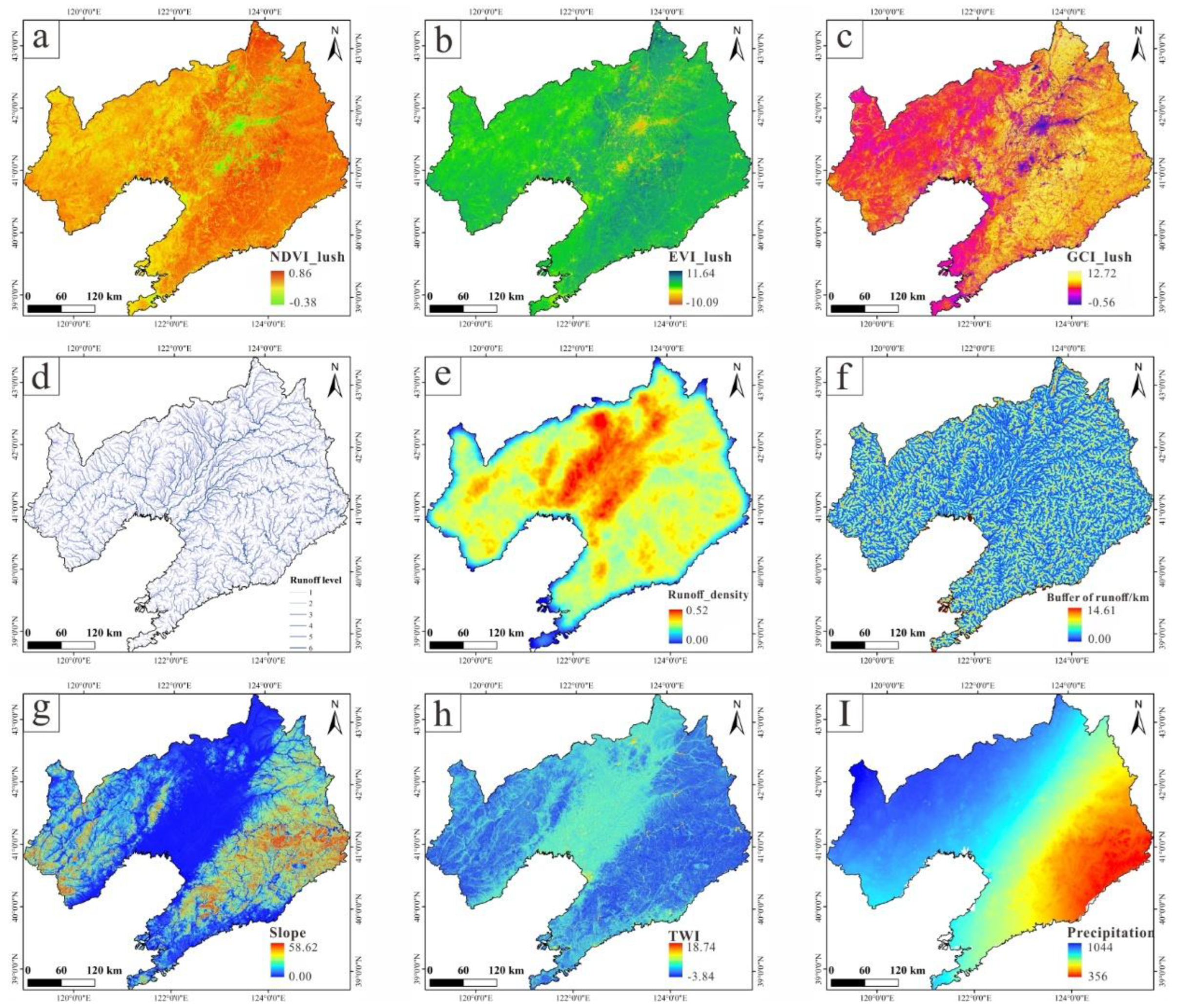
The spatial distributions of VIs_lush (NDVI, EVI and GCI) across Liaoning Province are shown in Figure A2(a), Figure A2(b), and Figure A2(c), respectively. To assess the effectiveness of VIs during the crop-lush period for SOC prediction, a comparative analysis was performed using VIs from both the bare-soil period and the crop-lush period. The results for VIs_lush, which are shown in Figure A1(d), Figure A1(e), and Figure A1(f), provide a foundation for model selection and validate the contribution of VIs to SOC content inversion.
Surface runoff pathways were derived via the D8 flow direction algorithm applied to the DEM data, as shown in Figure A2(d). On the basis of these pathways, two additional hydrological features were extracted, namely, surface runoff density (SRD) and surface runoff buffer (SRB), as presented in Figure A2(e) and Figure (f), respectively.
Furthermore, the topographic wetness index (TWI) was calculated to quantify the potential for water accumulation on the basis of the terrain features. The TWI is widely employed as a terrain-derived proxy for surface soil moisture distribution and runoff potential, both of which are closely linked to SOC variability. The TWI was computed as follows:
Where CA is the upslope contributing area (flow accumulation), and denotes the local slope angle. The spatial distribution of the TWI values in Liaoning Province is shown in Figure A1(h).
2.3.3. SOC Content Quantitative Inversion Model
Based on the analytical framework, a quantitative inversion model for SOC content in croplands across Liaoning Province was constructed. The model integrates both direct observation factors and indirect influencing factors, as summarized in Table 2. Corresponding GIS-based spatial distribution layers for each controlling variable are illustrated in Figure A1 and Figure A2.
2.4. Modelling Strategy
2.4.1. Ensemble Learning Algorithms
Ensemble learning increases predictive and classification performance levels through the integration of multiple models. By combining weak learners into a strong composite model, compared with single-model approaches, ELMs improve generalization and reduce the risk of overfitting [62,63]. The two main strategies in ELMs are bagging and boosting (Figure 4). Bagging employs parallel computation and bootstrap sampling to create diverse training subsets. Each subset is used to train an independent model, and the final prediction is obtained through averaging or voting, which reduces variance and enhances accuracy [64]. In contrast, boosting follows a sequential training process. Each model focuses on correcting the errors of its predecessor by adjusting sample weights, thereby reducing bias over iterations [65,66].
The RF model is a classic bagging algorithm that is renowned for its robustness and high performance across diverse datasets [67]. Boosting methods include the AdaBoost model, which adaptively adjusts sample weights to increase the prediction accuracy[66], and the XGBoost model, which employs gradient-based optimization techniques to enhance the model performance [68,69].
a) Random forest
The random forest model, developed by Leo Breiman in 1996, is an ensemble learning algorithm that employs the bagging strategy [64]. It was further enhanced through the introduction of the random subspace method by Tinkham in 1998 [67,70], which increases model diversity by randomly selecting subsets of features for each tree. Multiple decision trees are constructed [71], and final predictions are generated by averaging individual tree outputs:
Where, M is the total number of decision trees, is the prediction from the t-tℎ tree, and is the final ensemble prediction.
The RF model is highly effective in feature selection, resilient to noise, and capable of parallel processing. However, it may underperform with biased datasets or when model parameters are not well tuned.
b) AdaBoost
The AdaBoost model provides an increased regression accuracy by iteratively training a series of weak learners. It adjusts the weights of training samples at each iteration, increasing the emphasis on the previous prediction error of its predecessor [72]. The final strong learner is a weighted combination of weak learners:
Where, denotes the final prediction, is the output from the -th regression model, and represents the weight assigned based on its predictive accuracy. The weight of each weak learner is computed based on its average loss , using:
Where, is the regression error of the -th weak learner. The sample weights are updated using:
Where,is the weight of sample at iteration , is the observed SOC content, and is the model prediction result for sample .
The AdaBoost model can capture complex nonlinear patterns, but its sensitivity to noisy observations and outliers remains a limitation in regression contexts.
c) XGBoost
The XGBoost model, developed by Chen and Guestrin [68], enhances traditional boosting techniques through second-order Taylor expansion of the loss function and the incorporation of regularization terms, which improves accuracy and reduces overfitting [63]:
Where, is the true SOC content, is the predicted value at the previous iteration, is the prediction from the new regression tree added at -th iteration , is a convex loss function, Is the regularization term that penalized model complexity, is the number of leaf nodes in the regression tree, is the score assigned to the -th leaf, And are regularization parameters that control tree complexity and weight magnitude, respectively.
In regression scenarios, the XGBoost model excels at modelling nonlinear relationships, mitigating overfitting, and managing high-dimensional input features efficiently.
2.4.2. SHapley Additive Explanations
To quantify the contribution of each input variable to the predicted SOC content, the SHAP framework was applied to the ELMs. The SHAP method originates from cooperative game theory, wherein it attributes the difference between a specific prediction and the average prediction to individual features [73]. On the basis of the foundational work of SHAP [74,75,76], this approach fairly allocates the model output among all features on the basis of their marginal contributions across all possible feature combinations.
Mathematically, the shapley value for feature is defined as:
Where, denotes the contribution of feature , is the set of all features, is any subset of not containing , ) and represent the model output for the subsets with and without feature , respectively. The term denotes the probability corresponding to various feature combinations. Therefore, the result obtained from the above expression represents the marginal contribution of feature to the final outputs.
When it comes to the total contribution of all features for each observation, The total prediction can be expressed as:
Where, represents the model outputs without any features, is the number of all features, and is the value of feature for the given observation.
2.4.3. Model Evaluation
To evaluate the ability of the three ELMs to predict the SOC content, we divided the SOC samples into a training dataset and a validation dataset at a 2:1 ratio. The final meta-model was trained using 10-fold cross-validation to tune and determine the optimal parameters of the model. The trained regression models were subsequently validated using a validation dataset, and their performance was evaluated through the Pearson correlation coefficient (R), coefficient of determination (R²), root mean square error (RMSE), ratio of performance to deviation (RPD) and ratio of performance to the interquartile distance (RPIQ) as follows:
Where is the number of inversion units, is the predicted value of the i-th inversion unit, is the true value of that inversion unit, is the mean of observed values, and is the mean of predicted values, IQR is the inter-quartile range of the observed values, calculated as the difference between the 75th percentile (Q3) and the 25th percentile (Q1), IQR = Q3-Q1.
Both R and R² reflect the goodness of fit of models; R is particularly useful for evaluating the linear association, whereas R² emphasizes the proportion of explained variance. The RMSE quantifies the average magnitude of prediction errors and is sensitive to large deviations due to the squared term. RPD is the ratio of the standard deviation of observed values to the RMSE, whereas the RPIQ relies on the interquartile range (IQR) instead of the standard deviation, making it more robust to outliers and skewed distributions. Smaller RMSE values, along with larger RPD and RPIQ values, indicate greater predictive ability of the model [77]. These metrics provide a comprehensive and complementary evaluation of model accuracy, robustness, and generalizability.
2.4.3. Three Modelling Strategies
In this study, three MSs were proposed on the basis of direct observation and indirect influencing factors (Table 3). These strategies were designed to evaluate and compare the predictive performance of VIs derived from different phenological stages as follows:
Modeling Strategy 1 (MS-1): VIs_lush are used along with other factors.
Modeling Strategy 2 (MS-2): VIs_bare are used in conjunction with the same set of additional factors.
Modeling Strategy 3 (MS-3): Modelling is conducted without VIs.
3. Results
3.1. Accuracy of the Different Modelling Strategies and Ensemble Learning Models
The predictive performance of the three ELMs under MS-1, MS-2, and MS-3 is shown in Figure 5 and Figure 6. A comparative analysis of these strategies indicates that the two VI-enhanced strategies (MS-1 and MS-2) provided a significantly enhanced model performance. Regardless of the ensemble algorithm used, MS-1 consistently provided the most accurate predictions. This finding demonstrates that incorporating vegetation information, especially from crop-lush periods, provides essential ecological insights and enhances the model's ability to capture spatial variations in SOC. Overall, the R² values of all three ELMs greatly increased with the addition of VIs.
Under MS-1, the XGBoost model achieved an R² value of 0.84, an RMSE of 2.22 g/kg, an RPD of 2.49 and an RPIQ of 3.25. In contrast, under MS-2, the performance decreased to an R² value of 0.79, an RMSE of 2.53 g/kg, an RPD of 2.18 and an RPIQ of 2.85. The accuracy further decreased under MS-3, with an R² value of 0.77, an RMSE of 2.63 g/kg, an RPD of 2.10 and an RPIQ of 2.74. These results show that compared with MS-3, the inclusion of VIs_bare under MS-2 increased the R² value of the XGBoost model by 2.60%, reduced the RMSE by 3.80%, increased the RPD by 3.81%, and enhanced RPIQ by 4.01%. The use of VIs_lush in MS-1 led to a 9.09% increase in R², a 15.59% decrease in RMSE, an 18.57% increase in the RPD, and an 18.61% increase in RPIQ. When MS-1 was compared with MS-2, the R² improved by 6.33%, the RMSE decreased by 4.00%, the RPD increased by 18.61%, and the RPIQ increased by 14.04%. These improvements highlight the high explanatory power of VIs, especially VIs_lush, in modelling SOC variability. With respect to the RF model, MS-1 yielded an R² value of 0.70, an RMSE of 3.04 g/kg, an RPD of 1.82, and an RPIQ of 2.37, which were noticeably better than those under MS-2 (R² = 0.67, RMSE = 3.17 g/kg, RPD = 1.74, and RPIQ = 2.27) and MS-3 (R² = 0.67, RMSE = 3.16 g/kg, RPD = 1.75, and RPIQ = 2.28). However, it is noteworthy that in the RF model, the results of MS-1 and MS-2 were quite close, with even slight decreases observed in some metrics (e.g., RMSE, RPD, and RPIQ). This suggests that using VIs_bare may not enhance SOC prediction in this case and might even introduce data redundancy. From MS-3 to MS-2, the R² remained unchanged, whereas from MS-2 to MS-1, the value increased by 4.48%. This further confirms that VIs_lush provide important information that is not captured by the terrain or soil texture variables alone. Although the AdaBoost model generally showed lower predictive ability, a similar pattern was observed. Its prediction results resembled those of the RF model, with little to no change in R², RMSE, RPD, or RPIQ from MS-3 to MS-2 but with slight improvements upon adding VIs_lush under MS-1. Specifically, R² increased from 0.33 (MS-3) to 0.34 (MS-1), representing a 3.03% improvement, the RMSE decreased from 4.53 g/kg to 4.51 g/kg (−0.44%), the RPD increased from 1.22 to 1.23 (+0.82%), and the RPIQ increased from 1.59 to 1.60 (+0.63%). These results again underscore the crucial role of VIs_lush in enhancing prediction accuracy, albeit with more modest gains in the AdaBoost model.
The 1:1 scatter plots in Figure 6 show that MS-1 yielded the best alignment between the predicted and observed SOC values, with data points distributed more symmetrically around the 1:1 line and a reduced bias observed in both the high- and low-SOC regions. In contrast, MS-3 showed marked underestimation at higher SOC levels and greater residual variance. The density-based heatmaps further support these findings: under MS-1, the predicted values were tightly clustered along the diagonal, indicating high agreement between the predictions and observations. This clustering decreased under MS-2 and was lowest under MS-3, where predictions deviated significantly, especially at high SOC levels.
In summary, the inclusion of VIs, particularly during periods of lush growth, substantially improved the predictive performance of the SOC models. MS-2, which incorporated VIs_bare, clearly proved more robust than the baseline MS-3 did, whereas MS-1, which used VIs_lush, emerged as the most scientifically grounded strategy for capturing cropland SOC variability. Among the three models, XGBoost made the most effective use of vegetation-related features, followed by the RF model, whereas AdaBoost was the least sensitive to VI input but still benefited from its inclusion.
3.2. Feature Analysis Based on the SHAP
Following the model performance evaluation, the XGBoost model was identified as the optimal model for determining the SOC content. To investigate the model’s internal decision logic, SHAP analysis was employed to interpret the contributions of individual features under MS-1, MS-2, and MS-3, as shown in Figure 7.
As shown in Figure 7, the SHAP summary plots under the three MSs demonstrate generally consistent rankings among most non-VIs. Key features, such as precipitation, DEM, SRD, and shortwave infrared bands (e.g., B7 and B5), consistently emerged as the top contributors across all the strategies. This consistency indicates the robustness and reliability of the model outputs under varying feature construction strategies. In contrast, differences were primarily observed in the ranking and presence of VIs, such as NDVI_lush and EVI_lush in MS-1 and their corresponding NDVI_bare and EVI_bare values under MS-2. These changes reflect the influence of temporal and contextual variations in vegetation information on SOC prediction, whereas the stable ranking of physical and topographic variables supports the validity of the adopted modelling strategies. Therefore, the relatively stable SHAP value distributions of non-VI features confirm that the ELMs are not overly sensitive to feature engineering choices, enhancing the interpretability and credibility of the inversion results.
Under MS-1 (Figure 7(a)(d)), VIs_lush and other vegetation indices were among the top-ranked predictors, demonstrating strong correlations with the observed ecological patterns. These variables showed broad and dispersed SHAP distributions—for example, NDVI_lush ranged from approximately –2 to +2, with both positive and negative contributions. This suggests a strong and nonlinear regulatory role in SOC predictions, which aligns with ecological processes such as photosynthetic carbon input and litter deposition [32,78]. EVI_lush highlights the multidimensional influence of vegetation structure and function during peak biomass periods. Notably, in the MS-1 strategy, NDVI_lush and EVI-lush contribute significantly to the explanation of SOC, while the SHAP value of GCI_lush is zero. We speculate that this is due mainly to its high correlation with NDVI_lush and EVI_lush. In XGBoost-based tree models, when multiple features are highly correlated, the model tends to prioritize more representative or informative features for node splitting, which results in the contribution of related features being diluted or replaced. Therefore, although GCI_lush itself may contain information, owing to its high overlap with NDVI_lush and EVI_lush, the XGBoost model prioritizes NDVI_lush and EVI_lush when the tree structure is constructed, resulting in the SHAP value of GCI_lush reaching zero. In contrast, MS-2 (Figure 7(b)(e)), which included VIs_bare, exhibited narrow and centralized SHAP distributions, mostly within the interval of –1 to +1. Their marginal contributions were limited, reflecting the lack of vegetation information and reduced spectral heterogeneity during bare-soil periods. This restricts the ability of the model to capture key ecological drivers of SOC, such as biomass input or microbial activity. The MS-3 strategy (Figure 7(c)(f)), which excluded VIs_lush and VIs_bare and relied on topographic and climatic variables (e.g., DEM, slope, and precipitation). The absence of phenological indicators reduced the ecological sensitivity of the model and impaired its ability to capture biologically driven SOC variation.
From an ecological perspective, MS-1 provides a more complete representation of vegetation–topography–carbon cycle coupling. It involves the integration of more rational VIs, spectral bands, and environmental attributes, enabling the model to depict the spatial heterogeneity of SOC more accurately. In contrast, MS-2, which is dominated by bare soil reflectance and static terrain factors, lacks the biological cues necessary to fully characterize SOC processes. Consequently, its explanatory power and ecological depth are significantly constrained.
In summary, SHAP-based analysis highlights the superior predictive capacity and ecological relevance of vegetation indices derived from the lush period. These features enhance model interpretability and support more accurate and ecologically meaningful SOC mapping by incorporating seasonal vegetation dynamics during periods of high productivity.
3.2. Cropland SOC Content
On the basis of the evaluation results from the test datasets, the XGBoost regression model was identified as the optimal algorithm for SOC content prediction. Consequently, it was employed under both modelling strategies, MS-1, MS-2 and MS-3, to conduct regional-scale inversion and perform statistical analysis of the predicted SOC content across the entire study area (Table 4).
Via the use of the optimal modelling combination—the XGBoost model under MS-1—the spatial distribution of the SOC content across croplands in Liaoning Province was mapped (Figure 8). The results reveal a distinct spatial gradient in the SOC concentration, reflecting the combined effects of topography, climate, land use, and vegetation productivity across the region.
As shown in Figure 8, the SOC content ranged from 2.19 g·kg⁻¹ to 33.86 g·kg⁻¹, with a mean value of 13.08 g·kg⁻¹, indicating moderate organic matter levels overall. The distribution pattern clearly displays spatial heterogeneity. Eastern Liaoning exhibits the highest SOC concentrations, particularly in the hilly and mountainous regions of Dandong, Benxi, and eastern Anshan. These areas are marked in red to orange in the map and are characterized by high precipitation, dense vegetation cover, and limited anthropogenic disturbance—all favourable conditions for organic matter accumulation. The SOC concentrations here often exceed 25 g·kg⁻¹, indicating high soil fertility. Central Liaoning, including parts of Shenyang, Liaoyang, and western Anshan, has moderate SOC levels (approximately 10–20 g·kg⁻¹), depicted in light green to light blue. This region includes major agricultural zones with a mix of irrigated cropland and hilly terrain, where SOC levels are influenced by both land use intensity and slope-driven erosion. In western Liaoning, particularly around Chaoyang and Fuxin, the lowest SOC concentrations, mostly less than 10 g·kg⁻¹, are shown in dark blue in the map. These areas are generally drier, more degraded, and experience frequent soil erosion, leading to limited organic matter accumulation and lower soil productivity. Southern coastal areas, such as Dalian and Jinzhou, exhibit moderate to low SOC levels, which is likely due to intensive land use, saline soils, and urban expansion. Overall, the spatial pattern aligns well with known climatic gradients, with higher SOC in humid and vegetated eastern regions and lower SOC in arid and erosion-prone western zones. The map clearly delineates agroecological zoning and can inform soil fertility management, land degradation monitoring, and targeted conservation practices.
These results also validate the effectiveness of MS-1, in which vegetation indices from the lush season and environmental covariates are integrated, in capturing the spatial variability of SOC across complex landscapes.
4. Discussion
This study provides a refined approach to estimate the SOC content in croplands using remote sensing and ELMs. Through model optimization, innovative feature selection, and comparative analysis, the proposed methodology demonstrates both theoretical significance and practical applicability. The following discussion elaborates on the methodological advances, model performance, and inherent limitations.
4.1. Innovation in Feature Selection and Modelling Strategy
The superior performance of MS-1 compared with MS-2 and MS-3 (Section 3.2) indicates that replacing bare-soil VIs with those derived from the crop-lush period is a key factor driving the increase in the SOC inversion accuracy. Previous studies have frequently relied on Vis, such as the NDVI and EVI, in SOC modelling, but most have relied on indices extracted from the bare-soil period [3,16,26,42,79,80,81]. However, such indices often neglect ecological dynamics during vegetation growth periods, which are more indicative of organic matter input. In this study, we proposed a novel strategy involving replacing bare-soil VIs (VIs_bare) with those from the crop-lush period (VIs_lush), guided by pedological theory on SOC formation. This approach yielded notable improvements in model performance. The vegetation density during the lush period is positively correlated with SOC, as denser vegetation generally contributes more plant litter and organic residues [82,83], thereby increasing the potential for the accumulation of SOC. VIs_lush, which reflect cumulative vegetation productivity during crop-lush periods, thus acts as an indirect proxy for SOC, integrating long-term effects of SOC on plant performance [84]. In contrast, VIs_bare primarily capture transient surface conditions and are more susceptible to non-SOC factors, such as soil moisture and roughness, which explains the lower accuracy of MS-2. Nonetheless, the reliability of VIs_lush is partially constrained by anthropogenic influences, such as fertilization and crop management [85]. Thus, while the use of VIs_lush enhances the predictive power, their effectiveness is context dependent and may not be universally applicable. Future research should assess this approach across different land use types to validate its robustness.
The SHAP dependence plots (Figure 9) further reveal the differences in contribution between bare-soil and crop-lush period VIs. NDVI_lush and EVI_lush exhibited clear and positive SHAP values, reflecting strong and consistent relationships with the SOC content. In contrast, their bare-soil counterparts showed weaker and more scattered relationships, indicating reduced predictive ability. Notably, GCI_lush exhibited SHAP values close to zero across the range of index values. Although the chlorophyll content, particularly as captured by GCI_lush, is mechanistically related to SOC through its link to photosynthetic capacity and biomass production, its predictive role in our models was minimal. This is likely due to the high correlation of GCI_lush with NDVI_lush and EVI_lush (Figure 10), resulting in information redundancy; consequently, the model prioritized NDVI_lush and EVI_lush for node splitting during training.
These findings underscore the importance of considering feature intercorrelations when modelling strategies are designed, as highly correlated variables may be downweighted despite their ecological relevance. Overall, our findings highlight that vegetation indices from the crop-lush period not only provide stronger and more interpretable signals for SOC prediction than their bare-soil counterparts do but also capture essential ecological processes underpinning SOC formation that static terrain or soil properties alone cannot represent.
4.2. Model Performance and Remote Sensing Data Considerations
Among the three ELMs tested, the XGBoost model consistently outperformed the RF and AdaBoost models following appropriate data preprocessing and hyperparameter tuning. Its iterative optimization mechanism effectively reduces prediction variance and handles structured datasets [68]. The performance hierarchy observed (XGBoost > RF > AdaBoost) agrees with findings from related studies [25,80], including recent SOC inversion research conducted in Liaoning Province within Northeast China, thereby reinforcing the reliability of the results of this study [44,79].
Methodologically, the dominance of the XGBoost model conforms with its ability to model nonlinear relationships and complex feature interactions, making it well suited for capturing the complex feedback loops among SOC, vegetation growth, and VIs_lush. This highlights the utility of ensemble learning in disentangling the multivariate drivers of SOC variability. However, model efficacy remains context-specific and is influenced by dataset characteristics, including class imbalance and noise levels. With respect to data sources, the accuracy of SOC inversion is also influenced by the spatial, temporal, and spectral resolution of remote sensing imagery. High-spatial-resolution platforms (e.g., Landsat and Sentinel-2) often suffer from low revisit frequencies, causing seamline mismatches in large-area mosaicking. Integrating multitemporal data can help mitigate these limitations and increase model stability.
Moreover, hyperspectral data—offered by several platforms, including Gaofen-5 and EnMAP—hold great promise for enhancing the accuracy of SOC prediction. Laboratory and field-based studies have validated the spectral sensitivity of SOC, and future efforts should prioritize the fusion of multispectral and hyperspectral observations for large-scale SOC content mapping [14,86].
4.3. Study Limitations
The proposed crop-lush period VI modelling strategy was evaluated primarily in cropland settings. However, in agricultural systems, SOC–vegetation relationships are often distorted by human interventions [52], such as fertilization and residue incorporation [55]. These factors can mask the natural feedback loop between vegetation and SOC. In contrast, forest ecosystems, which rely on natural processes, such as litterfall and root decay, may benefit more from crop-lush VIs in SOC inversion [32,33,87]. Thus, future work should include forest sampling to assess the transferability of this approach. In terms of the five principal soil-forming factors [88], incorporating temporal dynamics into SOC inversion poses a significant challenge. Accurate SOC content inversion requires the integration of both spatial heterogeneity and temporal dynamics. While topography and meteorological variables were incorporated in our approach, it did not account for temporally variable factors such as land use change and soil formation. Addressing these aspects could significantly enhance model reliability. Furthermore, the current model does not differentiate between paddy and upland fields—land use types with distinct carbon cycles. The incorporation of high-resolution land cover classification and time-sensitive predictors may reduce spatial uncertainty and improve prediction accuracy across diverse agroecosystems.
In this study, approximately 468 sample points were initially collected, and their uneven spatial distribution limited the generalizability of the model. To compensate, we applied kriging interpolation to augment the dataset to 2,799 samples. Although this increased spatial coverage, it also introduced interpolation-based uncertainties that may affect model fidelity. Future research should expand field sampling to establish a more robust training dataset.
5. Conclusions
In this study, we proposed an optimized modelling strategy for regional-scale SOC content estimation by integrating machine learning and remote sensing and recommended the replacement of bare-soil VIs with those from the crop-lush period. A cropland case study in Liaoning Province, Northeast China, demonstrated that distinguishing directly observed from indirectly influencing factors and prioritizing VIs_lush over VIs_bare significantly increased the accuracy of the SOC inversion. Among the three ELMs, the XGBoost model showed the highest sensitivity to VIs and achieved the best performance under MS-1 (R² = 0.84, RMSE = 2.22 g/kg, RPD = 2.49, and RPIQ = 3.25), followed by the RF model, whereas AdaBoost was less sensitive but still benefited from VIs_lush. SHAP analysis for MS-1, MS-2, and MS-3 confirmed the critical role of VIs_lush, revealing that vegetation conditions during the crop-lush period capture essential SOC variability beyond static terrain or soil features. The inversion results indicated an east–west SOC gradient, with higher values in the eastern mountainous and coastal areas and lower values in the central and western sandy regions (mean: 13.08 g/kg; range: 2.19–33.86 g/kg). This method supports long-term, large-scale SOC monitoring and provides valuable references for soil surveillance, crop planning, precision fertilization, sustainable land management, soil health assessment, and carbon cycling research.
Author Contributions
Conceptualization, Q.Z. and Y.F.; Methodology, Q.Z., Y.F. and H.D.; Software, Q.Z. and W.H.; Validation, H.D. and N.F.; Formal analysis, G.L.; Investigation, G.L.; Resources, C.W. and G.L.; Data curation, C.W., G.L., and A.W.; Writing—original draft preparation, Q.Z.; Writing—review and editing, Y.F.; Visualization, Q.Z. and Z.Q.; Supervision, Y.F.; Project administration, Y.F.; Funding acquisition, Y.F. All authors have read and agreed to the published version of the manuscript.
Funding
This research was funded by the National Key Research and Development Program of China (Grant No.2023YFD1500801, Grant No.2023YFD1500805), Liaoning Province Joint Fund Project (Grant No.2023-BSBA-313), Youth Innovation Promotion Association CAS to CW (2022194), the Liaoning Province Science and Technology Project (Grant No. 2022JH2/101300128) and Northeast Geological S&T Innovation Center of China Geological Survey (Grant No. QCJJ2022-21)
Data Availability Statement
The data used in this study can be accessed upon request from the corresponding author
Acknowledgments
We would like to thank the website for providing the data used in the paper and the editor and reviewers for their insightful comments.
Conflicts of Interest
The authors declare no conflicts of interest.
Appendix A
Figure A1.
Direct observation factors. (a) NDWI; (b)CI; (c)BI; (d)NDVI_bare; (e)EVI_bare; (f)GCI_bare.
Figure A1.
Direct observation factors. (a) NDWI; (b)CI; (c)BI; (d)NDVI_bare; (e)EVI_bare; (f)GCI_bare.
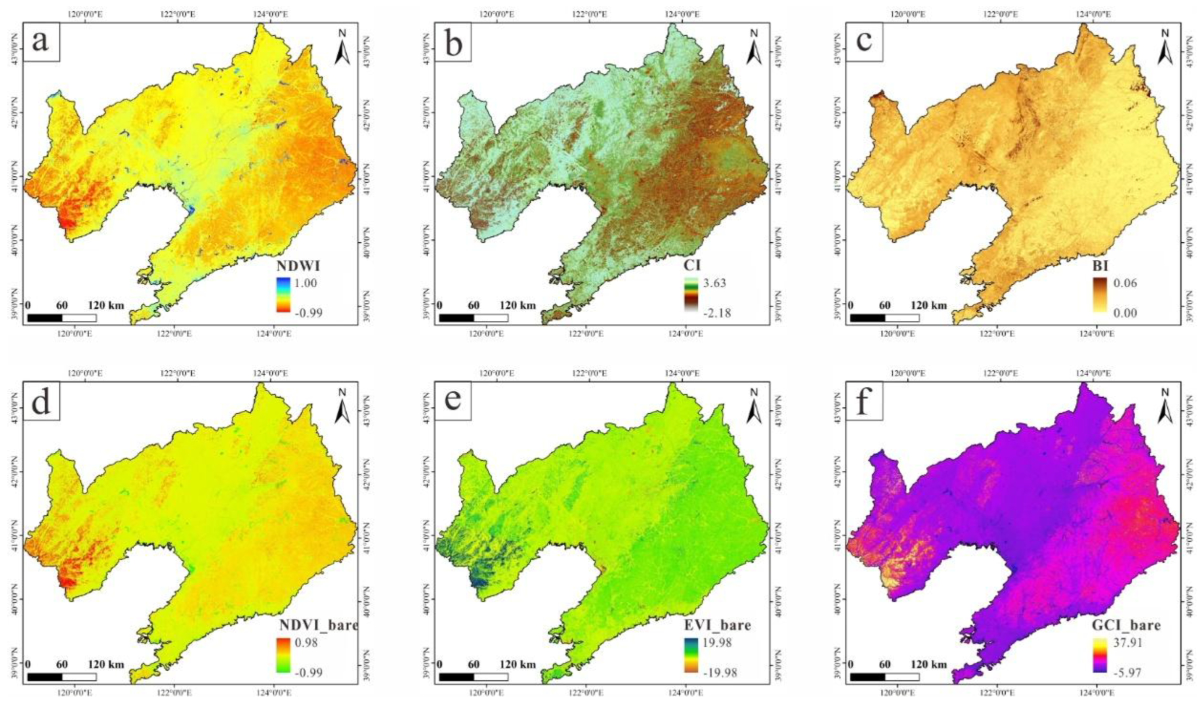
Figure A2.
Indirect influence factors used for SOC inversion in Liaoning Province: (a) NDVI during the crop-lush period; (b) EVI during the crop-lush period; (c) GCI during the crop-lush period; (d) Surface runoff path; (e) SRD; (f) SRB; (g) Slope; (h) TWI; (i) Annual precipitation in 2020.
Figure A2.
Indirect influence factors used for SOC inversion in Liaoning Province: (a) NDVI during the crop-lush period; (b) EVI during the crop-lush period; (c) GCI during the crop-lush period; (d) Surface runoff path; (e) SRD; (f) SRB; (g) Slope; (h) TWI; (i) Annual precipitation in 2020.
References
- Bongiorno, G.; Bünemann, E.K.; Oguejiofor, C.U.; Meier, J.; Gort, G.; Comans, R.; Mäder, P.; Brussaard, L.; de Goede, R. Sensitivity of labile carbon fractions to tillage and organic matter management and their potential as comprehensive soil quality indicators across pedoclimatic conditions in Europe. Ecological Indicators 2019, 99, 38–50. [Google Scholar] [CrossRef]
- Lorenz, K.; Lal, R.; Ehlers, K. Soil organic carbon stock as an indicator for monitoring land and soil degradation in relation to United Nations' Sustainable Development Goals. Land Degradation & Development 2019, 30. [Google Scholar] [CrossRef]
- Luo, C.; Zhang, W.; Zhang, X.; Liu, H. Mapping the soil organic matter content in a typical black-soil area using optical data, radar data and environmental covariates. Soil and Tillage Research 2024, 235, 105912. [Google Scholar] [CrossRef]
- Hicks Pries, C.E.; Castanha, C.; Porras, R.; Torn, M. The whole-soil carbon flux in response to warming. Science 2017, 355, 1420–1423. [Google Scholar] [CrossRef]
- Schmidt, M.W.; Torn, M.S.; Abiven, S.; Dittmar, T.; Guggenberger, G.; Janssens, I.A.; Kleber, M.; Kögel-Knabner, I.; Lehmann, J.; Manning, D.A. Persistence of soil organic matter as an ecosystem property. Nature 2011, 478, 49–56. [Google Scholar] [CrossRef]
- Poggio, L.; De Sousa, L.M.; Batjes, N.H.; Heuvelink, G.B.M.; Kempen, B.; Ribeiro, E.; Rossiter, D. SoilGrids 2.0: producing soil information for the globe with quantified spatial uncertainty. SOIL 2021, 7. [Google Scholar] [CrossRef]
- Meng, X.; Bao, Y.; Wang, Y.; Zhang, X.; Liu, H. An advanced soil organic carbon content prediction model via fused temporal-spatial-spectral (TSS) information based on machine learning and deep learning algorithms. Remote Sensing of Environment 2022, 280, 113166. [Google Scholar] [CrossRef]
- Sha, J.; Chen, P.; Chen, S. Characteristics analysis of soil spectrum response resulted from organic material. Research of Soil and Water Conservation 2003, 10, 21–25. [Google Scholar]
- Sha, J.; Li, X. Research on spatial distribution of land resources based on remote sensing information. Journal of China Agricultural Resources and Regional Planning 2003, 24, 10–13. [Google Scholar]
- Rossel, R.V.; Behrens, T. Using data mining to model and interpret soil diffuse reflectance spectra. Geoderma 2010, 158, 46–54. [Google Scholar] [CrossRef]
- Mathews, H.; Cunningham, R.; Petersen, G. Spectral reflectance of selected Pennsylvania soils. Soil Science Society of America Journal 1973, 37, 421–424. [Google Scholar] [CrossRef]
- Peng, J.; Zhang, Y.; Zhou, Q.; Liu, X.; Zhou, W. Spectral characteristics of soils in Hunan province as affected by removal of soil organic matter. Soils 2006, 38, 453–458. [Google Scholar]
- Liu, H.; Qiu, Q.; Wu, L.; Li, W.; Wang, B.; Zhou, Y. Few-shot learning for name entity recognition in geological text based on GeoBERT. Earth Science Informatics 2022, 15, 979–991. [Google Scholar] [CrossRef]
- Bao, Y.; Ustin, S.; Meng, X.; Zhang, X.; Guan, H.; Qi, B.; Liu, H. A regional-scale hyperspectral prediction model of soil organic carbon considering geomorphic features. Geoderma 2021, 403, 115263. [Google Scholar] [CrossRef]
- Guo, L.; Zhang, H.; Shi, T.; Chen, Y.; Jiang, Q.; Linderman, M. Prediction of soil organic carbon stock by laboratory spectral data and airborne hyperspectral images. Geoderma 2019, 337, 32–41. [Google Scholar] [CrossRef]
- Nguyen, T.T.; Pham, T.D.; Nguyen, C.T.; Delfos, J.; Archibald, R.; Dang, K.B.; Hoang, N.B.; Guo, W.; Ngo, H.H. A novel intelligence approach based active and ensemble learning for agricultural soil organic carbon prediction using multispectral and SAR data fusion. Science of The Total Environment 2022, 804, 150187. [Google Scholar] [CrossRef]
- Shi, Z.; Ji, W.; Viscarra Rossel, R.; Chen, S.; Zhou, Y. Prediction of soil organic matter using a spatially constrained local partial least squares regression and the C hinese vis–NIR spectral library. European Journal of Soil Science 2015, 66, 679–687. [Google Scholar] [CrossRef]
- Dou, X.; Wang, X.; Liu, H.; Zhang, X.; Meng, L.; Pan, Y.; Yu, Z.; Cui, Y. Prediction of soil organic matter using multi-temporal satellite images in the Songnen Plain, China. Geoderma 2019, 356, 113896. [Google Scholar] [CrossRef]
- Biney, J.K.M.; Vašát, R.; Bell, S.M.; Kebonye, N.M.; Klement, A.; John, K.; Borůvka, L. Prediction of topsoil organic carbon content with Sentinel-2 imagery and spectroscopic measurements under different conditions using an ensemble model approach with multiple pre-treatment combinations. Soil and Tillage Research 2022, 220, 105379. [Google Scholar] [CrossRef]
- Kerr, D.D.; Ochsner, T.E. Soil organic carbon more strongly related to soil moisture than soil temperature in temperate grasslands. Soil Science Society of America Journal 2020, 84, 587–596. [Google Scholar] [CrossRef]
- Hobley, E.; Wilson, B.; Wilkie, A.; Gray, J.; Koen, T. Drivers of soil organic carbon storage and vertical distribution in Eastern Australia. Plant and Soil 2015, 390, 111–127. [Google Scholar] [CrossRef]
- Meng, X.; Bao, Y.; Liu, J.; Liu, H.; Zhang, X.; Zhang, Y.; Wang, P.; Tang, H.; Kong, F. Regional soil organic carbon prediction model based on a discrete wavelet analysis of hyperspectral satellite data. International Journal of Applied Earth Observation and Geoinformation 2020, 89, 102111. [Google Scholar] [CrossRef]
- Mosleh, Z.; Salehi, M.H.; Jafari, A.; Borujeni, I.E.; Mehnatkesh, A. The effectiveness of digital soil mapping to predict soil properties over low-relief areas. Environmental monitoring and assessment 2016, 188, 1–13. [Google Scholar] [CrossRef]
- Page, K.L.; Dang, Y.P.; Dalal, R.C. The ability of conservation agriculture to conserve soil organic carbon and the subsequent impact on soil physical, chemical, and biological properties and yield. Frontiers in sustainable food systems 2020, 4, 31. [Google Scholar] [CrossRef]
- Fu, P.; Clanton, C.; Demuth, K.M.; Goodman, V.; Griffith, L.; Khim-Young, M.; Maddalena, J.; Lamarca, K.; Wright, L.A.; Schurman, D.W. Accurate Quantification of 0–30 cm Soil Organic Carbon in Croplands over the Continental United States Using Machine Learning. Remote Sensing 2024, 16. [Google Scholar] [CrossRef]
- Odebiri, O.; Odindi, J.; Mutanga, O. Basic and deep learning models in remote sensing of soil organic carbon estimation: A brief review. International Journal of Applied Earth Observation and Geoinformation 2021, 102, 102389. [Google Scholar] [CrossRef]
- Liu, Y.; Jiang, C.; Feng, A.; Xu, H.; Wang, Y.; Yin, Y.; Wang, C.; Xie, D.; Gao, B. A causal prediction method for soil organic carbon storage change estimation, with Shaanxi Province as a case study. Computers and Electronics in Agriculture 2025, 234, 110271. [Google Scholar] [CrossRef]
- Jin, X.; Song, K.; Du, J.; Liu, H.; Wen, Z. Comparison of different satellite bands and vegetation indices for estimation of soil organic matter based on simulated spectral configuration. Agricultural and Forest Meteorology 2017, 244, 57–71. [Google Scholar] [CrossRef]
- Yang, L.; Cai, Y.; Zhang, L.; Guo, M.; Li, A.; Zhou, C. A deep learning method to predict soil organic carbon content at a regional scale using satellite-based phenology variables. International Journal of Applied Earth Observation and Geoinformation 2021, 102, 102428. [Google Scholar] [CrossRef]
- Bandyopadhyay, P.K.; Saha, S.; Mani, P.K.; Mandal, B. Effect of organic inputs on aggregate associated organic carbon concentration under long-term rice–wheat cropping system. Geoderma 2010, 154, 379–386. [Google Scholar] [CrossRef]
- Spohn, M.; Bagchi, S.; Biederman, L.A.; Borer, E.T.; Bråthen, K.A.; Bugalho, M.N.; Caldeira, M.C.; Catford, J.A.; Collins, S.L.; Eisenhauer, N. The positive effect of plant diversity on soil carbon depends on climate. Nature Communications 2023, 14, 6624. [Google Scholar] [CrossRef] [PubMed]
- Dai, G.; Zhu, S.; Cai, Y.; Zhu, E.; Jia, Y.; Ji, C.; Tang, Z.; Fang, J.; Feng, X. Plant-derived lipids play a crucial role in forest soil carbon accumulation. Soil Biology and Biochemistry 2022, 168, 108645. [Google Scholar] [CrossRef]
- Ge, J.; Xu, W.; Xiong, G.; Zhao, C.; Li, J.; Liu, Q.; Tang, Z.; Xie, Z. Depth-dependent controls over soil organic carbon stock across Chinese shrublands. Ecosystems 2023, 26, 277–289. [Google Scholar] [CrossRef]
- Fox, G.A.; Sabbagh, G.; Searcy, S.; Yang, C. An automated soil line identification routine for remotely sensed images. Soil Science Society of America Journal 2004, 68, 1326–1331. [Google Scholar] [CrossRef]
- Mirzaee, S.; Ghorbani-Dashtaki, S.; Mohammadi, J.; Asadi, H.; Asadzadeh, F. Spatial variability of soil organic matter using remote sensing data. Catena 2016, 145, 118–127. [Google Scholar] [CrossRef]
- Li, Q.; Wang, C.; Zhang, W.; Yu, Y.; Li, B.; Yang, J.; Bai, G.; Cai, Y. Prediction of soil nutrients spatial distribution based on neural network model combined with goestatistics. The Journal of Applied Ecology 2013, 24, 459–466. [Google Scholar]
- Liu, H.; Zhao, C.; Wang, J.; Huang, W.; Zhang, X. Soil organic matter predicting with remote sensing image in typical blacksoil area of Northeast China. Transactions of the Chinese Society of Agricultural Engineering 2011, 27, 211–215. [Google Scholar]
- Wang, Q.; Wu, C.; Chen, K.; Ba, D.; Zhao, S.; Wei, Y.; Liu, J.; Su, X.; Zhang, X. Estimating topsoil organic matter in qinghai lake basin using multi-spectral remote sensing images. Soils 2019, 1, 160–167. [Google Scholar]
- Al-Anazi, A.; Gates, I.D. On the Capability of Support Vector Machines to Classify Lithology from Well Logs. Natural Resources Research 2010, 19, 125–139. [Google Scholar] [CrossRef]
- Sebtosheikh, M.A.; Salehi, A. Lithology prediction by support vector classifiers using inverted seismic attributes data and petrophysical logs as a new approach and investigation of training data set size effect on its performance in a heterogeneous carbonate reservoir. Journal of Petroleum Science and Engineering 2015, 134, 143–149. [Google Scholar] [CrossRef]
- Gomes, L.C.; Faria, R.M.; de Souza, E.; Veloso, G.V.; Schaefer, C.E.G.; Fernandes Filho, E.I. Modelling and mapping soil organic carbon stocks in Brazil. Geoderma 2019, 340, 337–350. [Google Scholar] [CrossRef]
- Green, J.K.; Seneviratne, S.I.; Berg, A.M.; Findell, K.L.; Stefan, H.; Lawrence, D.M.; Pierre, G. Large influence of soil moisture on long-term terrestrial carbon uptake. Nature 2020, 565, 476–479. [Google Scholar] [CrossRef]
- Lamichhane, S.; Kumar, L.; Wilson, B. Digital soil mapping algorithms and covariates for soil organic carbon mapping and their implications: A review. Geoderma 2019, 352, 395–413. [Google Scholar] [CrossRef]
- Luo, C.; Zhang, W.; Zhang, X.; Liu, H. Mapping soil organic matter content using Sentinel-2 synthetic images at different time intervals in Northeast China. International Journal of Digital Earth 2023, 16, 1094–1107. [Google Scholar] [CrossRef]
- Lou, H.; Ren, X.; Yang, S.; Hao, F.; Cai, M.; Wang, Y. Relations between Microtopography and Soil N and P Observed by an Unmanned Aerial Vehicle and Satellite Remote Sensing (GF-2). Polish journal of environmental studies 2021, 30. [Google Scholar] [CrossRef]
- Bai, S.; Pei, J.; Li, S.; An, T.; Wang, J.; Meng, F.; Xu, J. Temporal and spatial dynamics of soil organic matter and pH in cultivated land of Liaoning Province during the past 30 years. Chin. J. Soil Sci 2016, 636–644. [Google Scholar]
- Wang, C.; Wang, X.; Zhang, Y.; Morrissey, E.; Liu, Y.; Sun, L.; Qu, L.; Sang, C.; Zhang, H.; Li, G. Integrating microbial community properties, biomass and necromass to predict cropland soil organic carbon. Isme Communications 2023, 3, 86. [Google Scholar] [CrossRef]
- Wang, J.; Feng, C.; Hu, B.; Chen, S.; Hong, Y.; Arrouays, D.; Peng, J.; Shi, Z. A novel framework for improving soil organic matter prediction accuracy in cropland by integrating soil, vegetation and human activity information. Science of The Total Environment 2023, 903, 166112. [Google Scholar] [CrossRef] [PubMed]
- Ha, W.; Gowda, P.H.; Howell, T.A. A review of downscaling methods for remote sensing-based irrigation management: Part I. Irrigation Science 2013, 31, 831–850. [Google Scholar] [CrossRef]
- Taghizadeh-Mehrjardi; R.; Kerry; Nabiollahi; K. Digital mapping of soil organic carbon at multiple depths using different data mining techniques in Baneh region, Iran. Geoderma: An International Journal of Soil Science 2016. [CrossRef]
- Wiesmeier, M.; Urbanski, L.; Hobley, E.; Lang, B.; von Lützow, M.; Marin-Spiotta, E.; van Wesemael, B.; Rabot, E.; Ließ, M.; Garcia-Franco, N. Soil organic carbon storage as a key function of soils-A review of drivers and indicators at various scales. Geoderma 2019, 333, 149–162. [Google Scholar] [CrossRef]
- Terrer, C.; Phillips, R.P.; Hungate, B.A.; Rosende, J.; Pett-Ridge, J.; Craig, M.E.; van Groenigen, K.J.; Keenan, T.F.; Sulman, B.N.; Stocker, B.D. A trade-off between plant and soil carbon storage under elevated CO2. Nature 2021, 591, 599–603. [Google Scholar] [CrossRef]
- Fensholt, R.; Proud, S.R. Evaluation of Earth Observation based global long term vegetation trends — Comparing GIMMS and MODIS global NDVI time series. Remote Sensing of Environment 2012, 119, 131–147. [Google Scholar] [CrossRef]
- Lal, R. Soil carbon sequestration to mitigate climate change. Geoderma 2004, 123, 1–22. [Google Scholar] [CrossRef]
- Lal, R. Soil erosion and carbon dynamics. 2005, 81, 137–142. [Google Scholar] [CrossRef]
- Quinton, J.N.; Govers, G.; Van Oost, K.; Bardgett, R.D. The impact of agricultural soil erosion on biogeochemical cycling. Nature Geoscience 2010, 3, 311–314. [Google Scholar] [CrossRef]
- Ritchie, J.C.; Mccarty, G.W.; Venteris, E.R.; Kaspar, T.C. Soil and soil organic carbon redistribution on the landscape. Geomorphology 2007, 89, 163–171. [Google Scholar] [CrossRef]
- Garten, C.f.; Post, W.M.; Hanson, P.J.; Cooper, L.W. Forest soil carbon inventories and dynamics along an elevation gradient in the southern Appalachian Mountains. Biogeochemistry 1999, 45, 115–145. [Google Scholar] [CrossRef]
- Raich, J.W.; Schlesinger, W.H. The global carbon dioxide flux in soil respiration and its relationship to vegetation and climate. Tellus B 1992, 44, 81–99. [Google Scholar] [CrossRef]
- Wairiu, M.; Lal, R. Soil organic carbon in relation to cultivation and topsoil removal on sloping lands of Kolombangara, Solomon Islands. Soil and Tillage Research 2003, 70, 19–27. [Google Scholar] [CrossRef]
- Schillaci, C.; Braun, A.; Kropáek, J. Terrain analysis and landform recognition. Geomorphological techniques 2015, 1–18. [Google Scholar] [CrossRef]
- Mienye, I.D.; Sun, Y. A survey of ensemble learning: Concepts, algorithms, applications, and prospects. Ieee Access 2022, 10, 99129–99149. [Google Scholar] [CrossRef]
- Zhang, Q.; Chen, J.; Xu, H.; Jia, Y.; Chen, X.; Jia, Z.; Liu, H. Three-dimensional mineral prospectivity mapping by XGBoost modeling: a case study of the Lannigou gold deposit, China. Natural Resources Research 2022, 31, 1135–1156. [Google Scholar] [CrossRef]
- Breiman, L. Bagging predictors. Machine learning 1996, 24, 123–140. [Google Scholar] [CrossRef]
- Ferreira, A.J.; Figueiredo, M.A. Boosting algorithms: A review of methods, theory, and applications. Ensemble machine learning: Methods and applications 2012, 35–85. [Google Scholar] [CrossRef]
- Schapire, R.E.; Freund, Y. Boosting: Foundations and algorithms. Kybernetes 2013, 42, 164–166. [Google Scholar] [CrossRef]
- Breiman, L. Random forests. Machine learning 2001, 45, 5–32. [Google Scholar] [CrossRef]
- Chen, T.; Guestrin, C. Xgboost: A scalable tree boosting system. In Proceedings of the Proceedings of the 22nd acm sigkdd international conference on knowledge discovery and data mining, 2016; pp. 785-794.
- Prokhorenkova, L.; Gusev, G.; Vorobev, A.; Dorogush, A.V.; Gulin, A. CatBoost: unbiased boosting with categorical features. Advances in neural information processing systems 2018, 31. [Google Scholar]
- Breiman, L.; Friedman, J.H.; Olshen, R.A.; Stone, C.J. Classification and regression trees; Routledge: 2017.
- Chen, J.; Mao, X.; Liu, Z.; Deng, H. Three-dimensional Metallogenic Prediction Based on Random Forest Classification Algorithm for the Dayingezhuang Gold Deposit. Geotectonica et Metallogenia 2020, 44, 231–241. [Google Scholar]
- Freund, Y.; Schapire, R.E. A decision-theoretic generalization of on-line learning and an application to boosting. Journal of computer and system sciences 1997, 55, 119–139. [Google Scholar] [CrossRef]
- Padarian, J.; Mcbratney, A.B.; Minasny, B. Game theory interpretation of digital soil mapping convolutional neural networks. SOIL 2020, 6, 389–397. [Google Scholar] [CrossRef]
- Shapley, L.S. A value for n-person games. Contributions to the Theory of Games 1953. [Google Scholar] [CrossRef]
- Liu, Y.; Du, H. The Built Environment and Urban Vibrancy: A Data-Driven Study of Non-Commuters’ Destination Choices Around Metro Stations. Land 2025, 14, 1619. [Google Scholar] [CrossRef]
- Zhao, J.; Jia, B.; Wu, J.; Wu, X. Study of Spatial and Temporal Characteristics and Influencing Factors of Net Carbon Emissions in Hubei Province Based on Interpretable Machine Learning. Land 2025, 14, 1255. [Google Scholar] [CrossRef]
- Bellon-Maurel, V.; Fernandez-Ahumada, E.; Palagos, B.; Roger, J.M.; Mcbratney, A. Critical review of chemometric indicators commonly used for assessing the quality of the prediction of soil attributes by NIR spectroscopy. 2019. [CrossRef]
- Ge, J.; Xu, W.; Xiong, G.; Zhao, C.; Li, J.; Liu, Q.; Tang, Z.; Xie, Z. Depth-Dependent Controls Over Soil Organic Carbon Stock across Chinese Shrublands. Ecosystems 2022, 26, 277–289. [Google Scholar] [CrossRef]
- Meng, X.; Bao, Y.; Luo, C.; Zhang, X.; Liu, H. SOC content of global Mollisols at a 30 m spatial resolution from 1984 to 2021 generated by the novel ML-CNN prediction model. Remote Sensing of Environment 2024, 300, 113911. [Google Scholar] [CrossRef]
- Zhang, Y.; Kou, C.; Liu, M.; Man, W.; Li, F.; Lu, C.; Song, J.; Song, T.; Zhang, Q.; Li, X. Estimation of Coastal Wetland Soil Organic Carbon Content in Western Bohai Bay Using Remote Sensing, Climate, and Topographic Data. Remote Sensing 2023, 15. [Google Scholar] [CrossRef]
- Liu, H.; Zhang, M.; Yang, H.; Zhang, X.; Meng, X.; Li, H.; Tang, H. Invertion of cultivated soil organic matter content combining multi-spectral remote sensing and random forest algorithm. Transactions of the Chinese Society of Agricultural Engineering 2020, 36, 134–140. [Google Scholar] [CrossRef]
- Angst, G.; Mueller, K.E.; Castellano, M.J.; Vogel, C.; Wiesmeier, M.; Mueller, C.W. Unlocking complex soil systems as carbon sinks: multi-pool management as the key. Nature Communications 2023, 14. [Google Scholar] [CrossRef] [PubMed]
- Dou, P.; Wang, F.; Ma, Y.; Pang, M.; Lin, D. Response of litter carbon, nitrogen and phosphorus to simulated leaching. Chinese Science Bulletin 2018, 63. [Google Scholar] [CrossRef]
- Zhou, Y.; Chen, S.; Zhu, A.-X.; Hu, B.; Shi, Z.; Li, Y. Revealing the scale-and location-specific controlling factors of soil organic carbon in Tibet. Geoderma 2021, 382, 114713. [Google Scholar] [CrossRef]
- Miner, G.L.; Delgado, J.A.; Ippolito, J.A.; Stewart, C.E. Soil health management practices and crop productivity. Agricultural & Environmental Letters 2020, 5, e20023. [Google Scholar] [CrossRef]
- Wang, S.; Guan, K.; Zhang, C.; Lee, D.; Margenot, A.J.; Ge, Y.; Peng, J.; Zhou, W.; Zhou, Q.; Huang, Y. Using soil library hyperspectral reflectance and machine learning to predict soil organic carbon: Assessing potential of airborne and spaceborne optical soil sensing. Remote Sensing of Environment 2022, 271, 112914. [Google Scholar] [CrossRef]
- Pan, Y.; Birdsey, R.A.; Fang, J.; Houghton, R.; Kauppi, P.E.; Kurz, W.A.; Phillips, O.L.; Shvidenko, A.; Lewis, S.L.; Canadell, J.G. A large and persistent carbon sink in the world's forests. Science (New York, N.Y.) 2011, 333, 988–993. [Google Scholar] [CrossRef] [PubMed]
- Jenny, H. Factors of soil formation: a system of quantitative pedology; Courier Corporation: 1994.
Figure 1.
Study area (a) location of Liaoning Province; (b) cropland in Liaoning Province and soil samples.
Figure 1.
Study area (a) location of Liaoning Province; (b) cropland in Liaoning Province and soil samples.
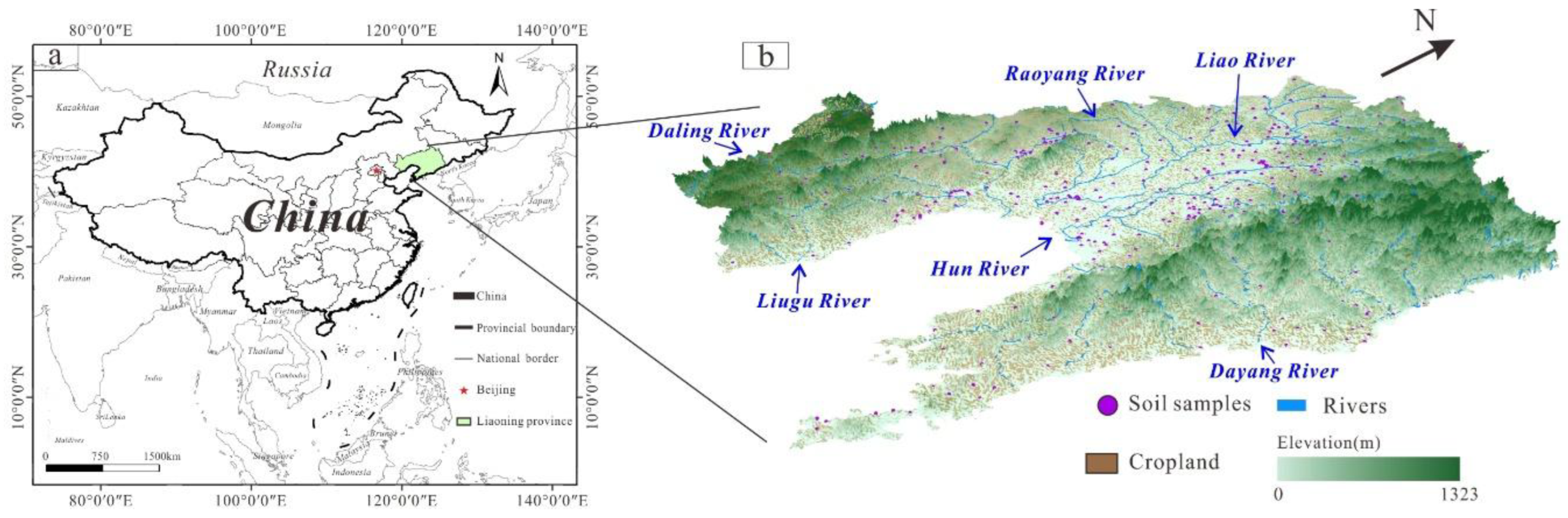
Figure 2.
RS images of the study area: (a) During the bare-soil period (April); (b) during the crop-lush period (August).
Figure 2.
RS images of the study area: (a) During the bare-soil period (April); (b) during the crop-lush period (August).
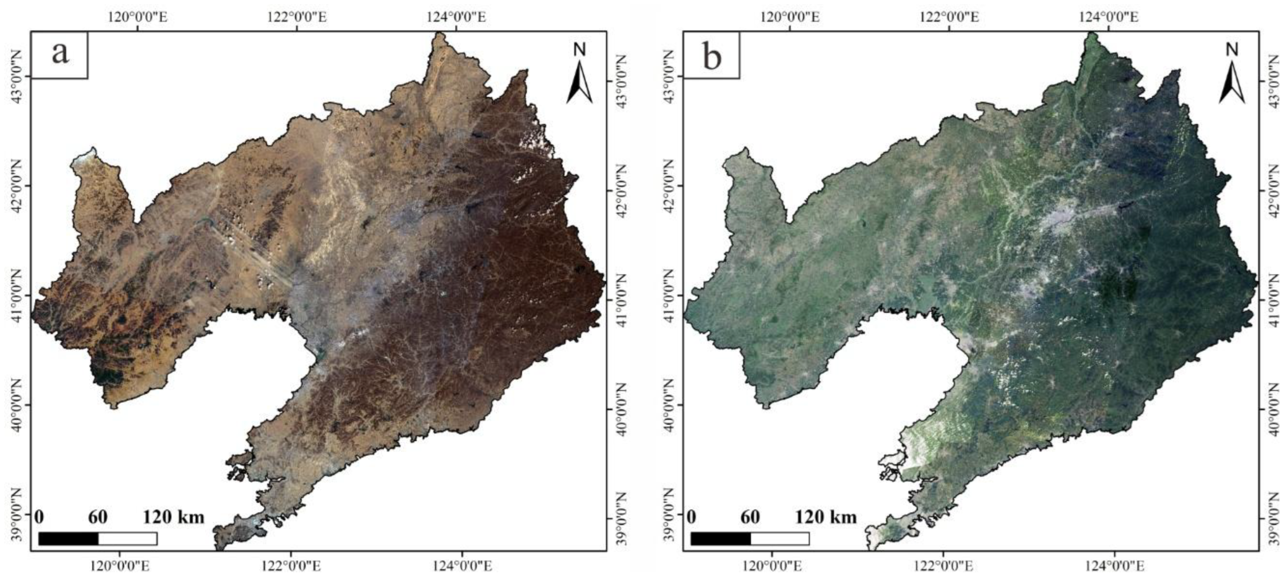
Figure 3.
Workflow of this study.
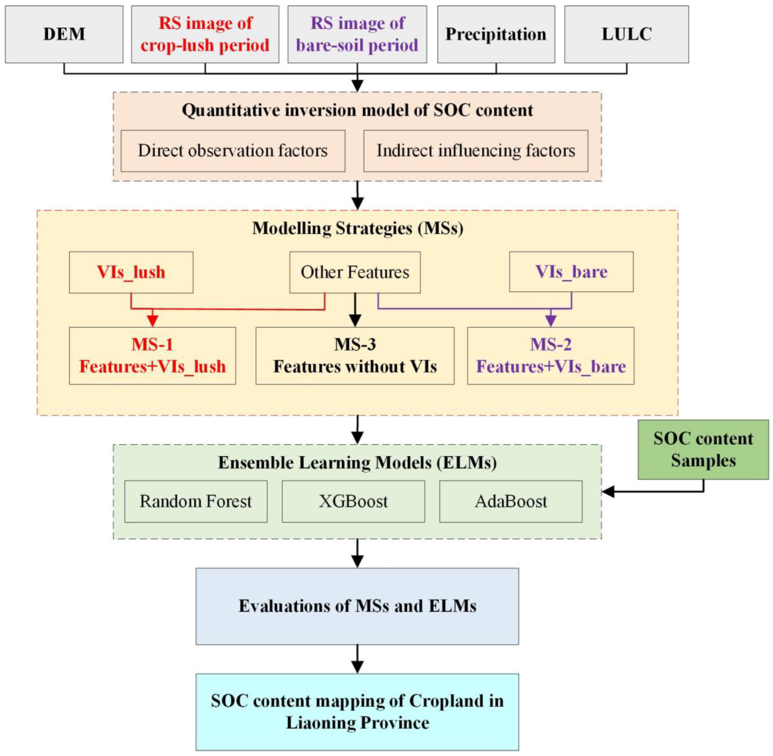
Figure 4.
Ensemble learning.
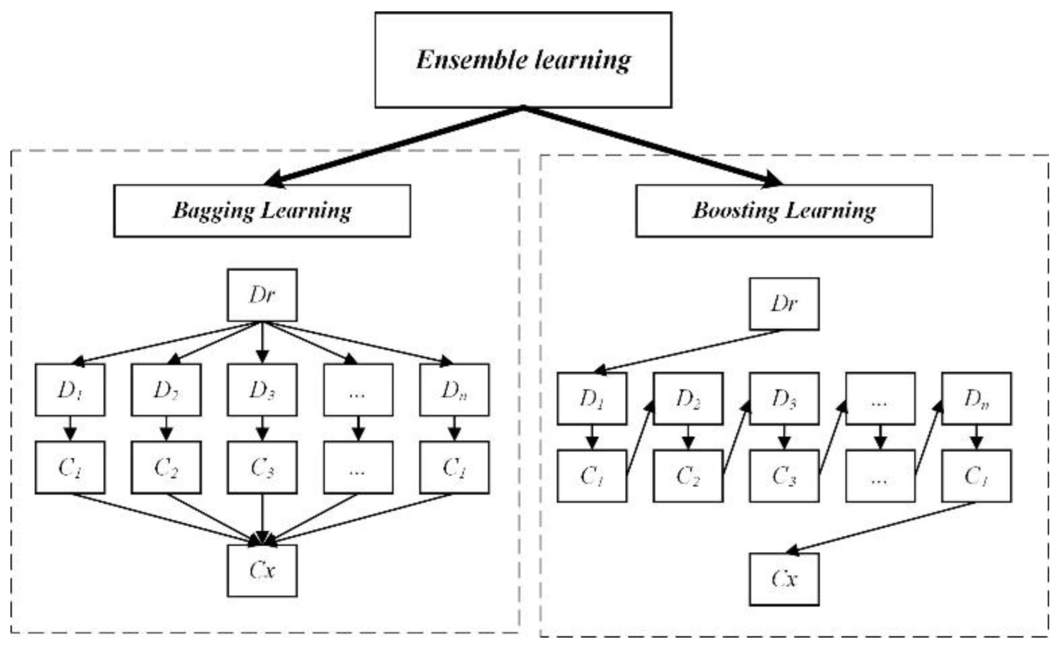
Figure 5.
Comparative performance of the XGBoost, RF, and AdaBoost models under MS-1, MS-2 and MS-3: (a) R², (b) RMSE, (c) RPD, and (d) RPIQ.
Figure 5.
Comparative performance of the XGBoost, RF, and AdaBoost models under MS-1, MS-2 and MS-3: (a) R², (b) RMSE, (c) RPD, and (d) RPIQ.
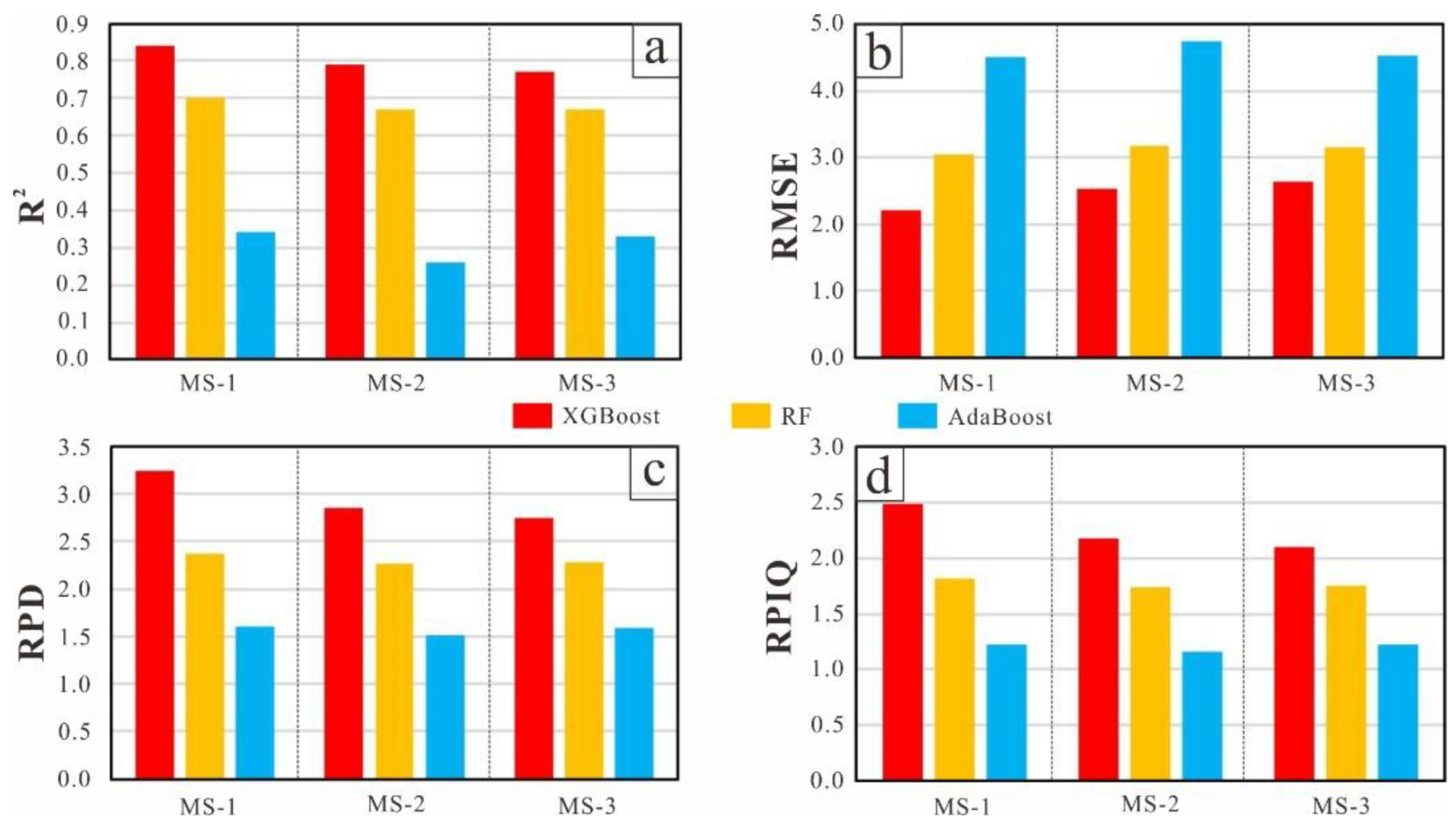
Figure 6.
Comparison of the performance of the XGBoost, RF, and AdaBoost models under MS-1 (a–c), MS-2 (d–f), and MS-3 (g–i) for mapping the SOC content based on observed versus predicted values.
Figure 6.
Comparison of the performance of the XGBoost, RF, and AdaBoost models under MS-1 (a–c), MS-2 (d–f), and MS-3 (g–i) for mapping the SOC content based on observed versus predicted values.
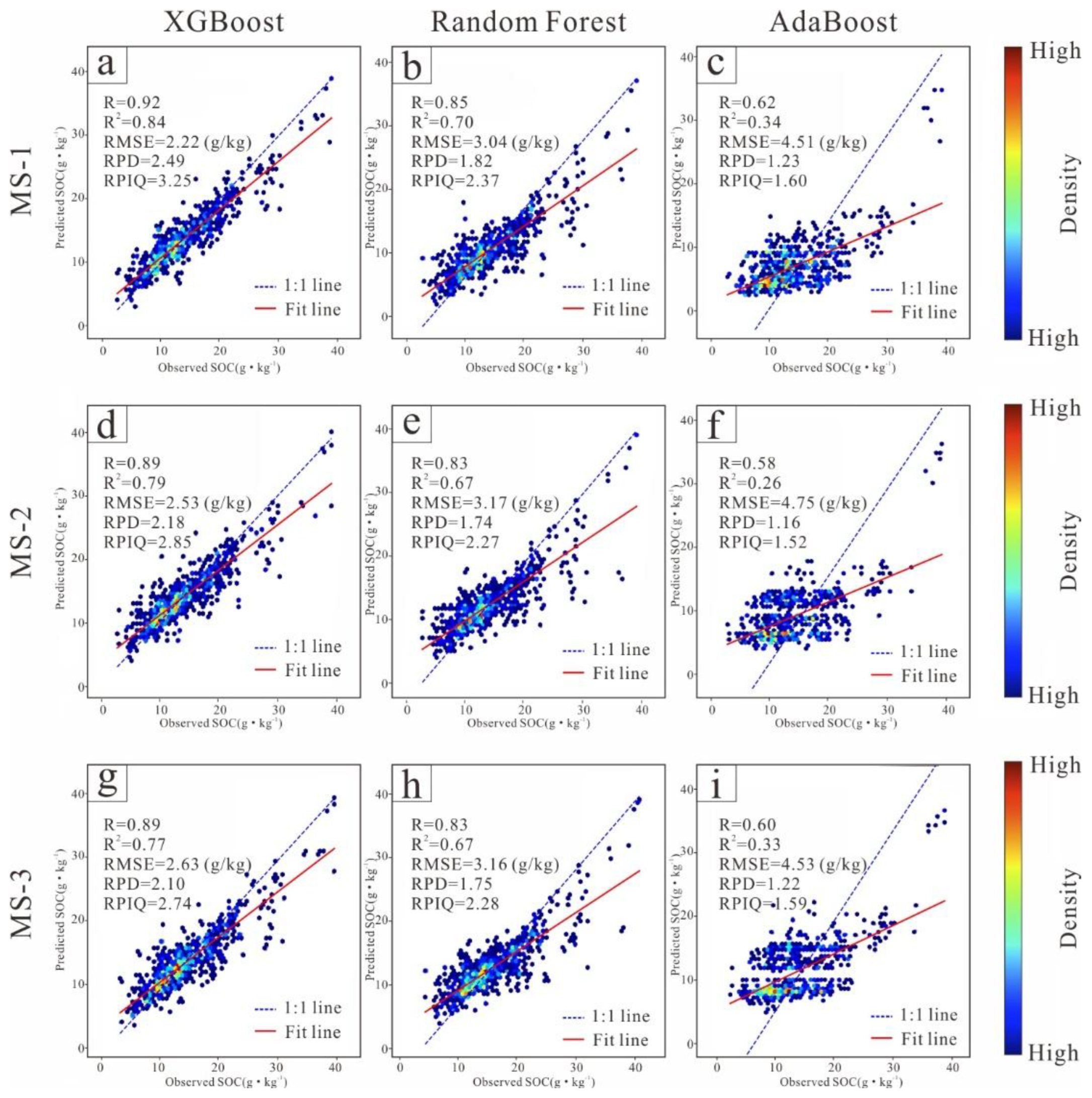
Figure 7.
Comparison of the distributions of the SHAP values for MS-1 (a) and (d), MS-2 (b) and (e), and MS-3 (c) and (f).
Figure 7.
Comparison of the distributions of the SHAP values for MS-1 (a) and (d), MS-2 (b) and (e), and MS-3 (c) and (f).
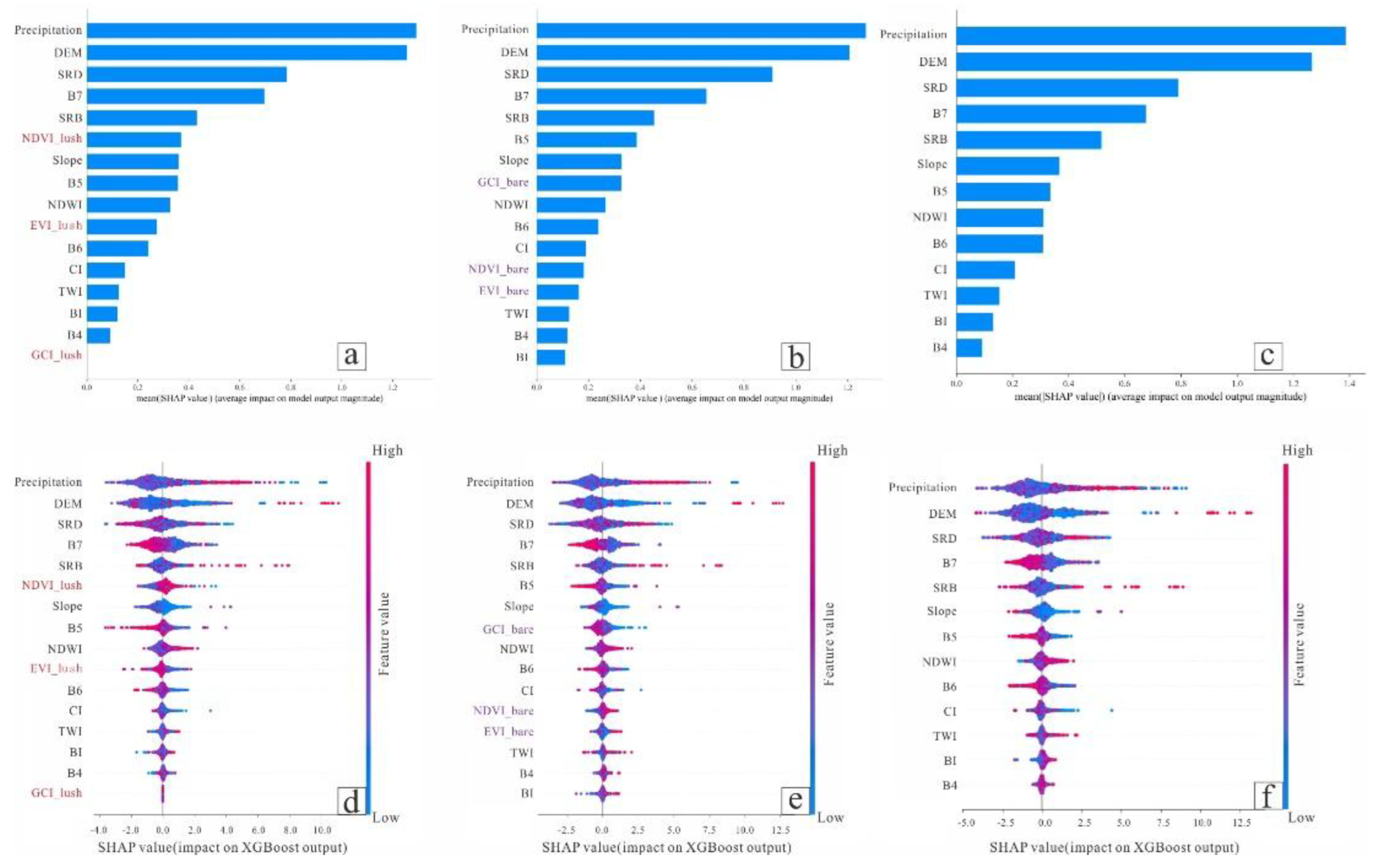
Figure 8.
Spatial distribution of inverted SOC content values in croplands of Liaoning Province using the XGBoost model under MS-1.
Figure 8.
Spatial distribution of inverted SOC content values in croplands of Liaoning Province using the XGBoost model under MS-1.
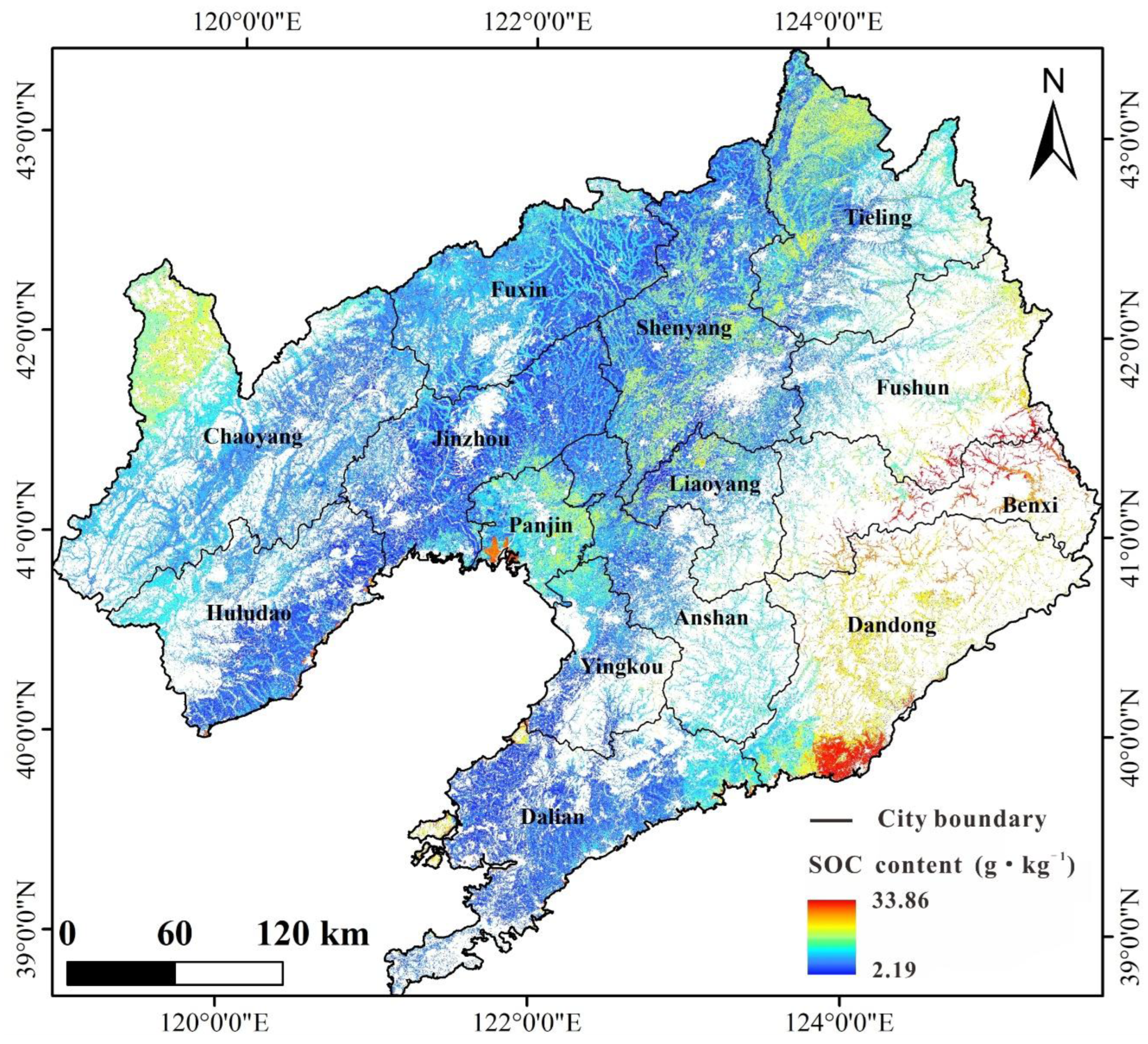
Figure 9.
SHAP dependence plots of (a)NDVI_lush, (b)EVI_lush, (c)GCI_lush, (d)NDVI_bare, (e)EVI_bare and (f)GCI_bare.
Figure 9.
SHAP dependence plots of (a)NDVI_lush, (b)EVI_lush, (c)GCI_lush, (d)NDVI_bare, (e)EVI_bare and (f)GCI_bare.
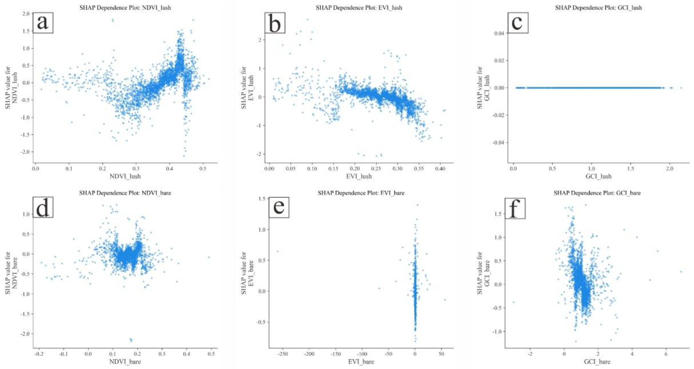
Figure 10.
Linear correlation between (a) GCI_lush and NDVI_lush and (b) EVI_lush.
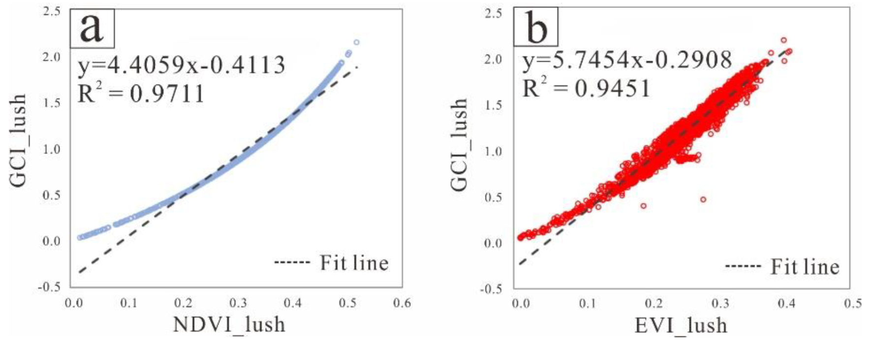

Table 1.
Statistical summary of SOC content samples collected and after data processing (g·kg-1).
| Types | Number of samples | Minimum | Maximum | Average | Standard deviation |
|---|---|---|---|---|---|
| Collected | 468 | 5.20 | 37.81 | 13.47 | 5.00 |
| After processing | 2,799 | 2.43 | 38.90 | 13.48 | 5.52 |
Table 2.
Inversion model for the SOC content in cropland in Liaoning Province.
| Major category | Factors type | Factors |
|---|---|---|
| Direct observation factors | Spectral reflectance and mathematical transformation | Ri |
| Soil properties during the bare-soil period | BI, NDWI, CI | |
| Indirect influencing factors | VIs during the crop-lush period | NDVI, EVI, GCI |
| Surface runoff conditions | SRD, SRB | |
| Terrain | DEM, Slope, TWI | |
| Climate | Precipitation |
* Ri represents the reflectance of the -th band.
Table 3.
Different modeling strategies.
| Feature types | Feature number | Modeling strategy 1 (MS-1) |
Modeling strategy 2 (MS-2) |
Modeling strategy 3 (MS-3) |
|---|---|---|---|---|
| Direct observation factors | Feature1 | |||
| Feature2 | SI | SI | SI | |
| Feature3 | BI | BI | BI | |
| Feature4 | Precipitation | Precipitation | Precipitation | |
| Indirect influencing factors | Feature5 | DEM | DEM | DEM |
| Feature6 | Slope | Slope | Slope | |
| Feature7 | TWI | TWI | TWI | |
| Feature8 | SRD | SRD | SRD | |
| Feature9 | SRB | SRB | SRB | |
| Feature10 | NDVI_lush | NDVI_bare | \ | |
| Feature11 | EVI_lush | EVI_bare | \ | |
| Feature12 | GCI_lush | GCI_bare | \ |
* represents the reflectance of the -th spectral band.
Table 4.
Summary statistics of the SOC inversion results using the XGBoost model under MS-1, MS-2 and MS-3.
Table 4.
Summary statistics of the SOC inversion results using the XGBoost model under MS-1, MS-2 and MS-3.
| Statistic | MS-1(g·kg-1) | MS-2(g·kg-1) | MS-3(g·kg-1) |
|---|---|---|---|
| Minimum | 2.19 | 1.56 | 1.98 |
| Maximum | 33.86 | 33.60 | 35.65 |
| Average | 13.08 | 12.73 | 14.15 |
| Median | 12.53 | 12.74 | 12.85 |
| Standard Deviation | 3.13 | 3.29 | 3.31 |
Disclaimer/Publisher’s Note: The statements, opinions and data contained in all publications are solely those of the individual author(s) and contributor(s) and not of MDPI and/or the editor(s). MDPI and/or the editor(s) disclaim responsibility for any injury to people or property resulting from any ideas, methods, instructions or products referred to in the content. |
© 2025 by the authors. Licensee MDPI, Basel, Switzerland. This article is an open access article distributed under the terms and conditions of the Creative Commons Attribution (CC BY) license (http://creativecommons.org/licenses/by/4.0/).
Copyright: This open access article is published under a Creative Commons CC BY 4.0 license, which permit the free download, distribution, and reuse, provided that the author and preprint are cited in any reuse.


