
Submitted:
12 May 2025
Posted:
13 May 2025
You are already at the latest version
Abstract
Mapping Soil Organic Carbon (SOC) at a regional scale is essential for assessing soil health and supporting sustainable land management. This study evaluates the potential of using Sentinel-2 imagery and regional calibration to predict SOC in salt-affected agricultural lands in Portugal, while also assessing the influence of soil properties, such as salinity, on SOC prediction. A per-pixel mosaicking approach was set to analyze the relation of spectral reflectance indices linked to bare soil conditions with SOC. SOC prediction models were developed using Linear Regression (LR) and Partial Least Squares Regression (PLSR). Among the tested approaches, the combination of maximum Bare Soil Index (maxBSI) with LR produced the most accurate SOC predictions, achieving moderate prediction performance (R² = 0.52, RMSE = 0.16%). This approach slightly outperformed the application of the 90th percentile of bare soil pixels (R90 reflectance) and the median approaches with PLSR. Notably, our findings indicate that soil salinity did not significantly affect SOC predictions, suggesting that within the observed salinity range of ECe between 1.2 and 10.4 dS m⁻¹ in topsoil, salinity had no statistical influence on SOC prediction. However, further case studies are needed to validate this observation across diverse agricultural conditions. In contrast, soil texture and moisture content emerged as the dominant factors influencing soil reflectance. This study demonstrates that Sentinel-2-derived indices, particularly maxBSI, combined with the proposed regional calibration approach, can be a cost-effective and scalable solution to monitor and regularly update SOC maps.
Keywords:
Soil organic carbon
; Sentinel-2 imagery
; Temporal mosaic
; Regional Calibration
; Soil salinity
; STEROPES project
1. Introduction
Soil Organic Carbon (SOC) is one of the most critical indicators of soil health and fertility, playing an important role in the productivity and sustainability of agricultural ecosystems. SOC contributes to soil structure, water retention, nutrient cycling, and microbial activity, all of which are essential for promoting crop yield and soil resilience against environmental stresses such as drought and erosion [1,2]. Along with its role in agricultural systems adaptation to climate change, SOC can play a role in climate mitigation by sequestering atmospheric carbon [3]. The assessment and increase or conservation of SOC are therefore key priorities for both farmers and policymakers who seek to enhance agricultural productivity while preserving ecosystem health. However, assessing SOC over large spatial scales presents significant challenges. Traditional soil sampling and laboratory analyses are resource-intensive and time-consuming, particularly when applied across large agricultural regions.
Recent advancements in remote sensing technologies, particularly the availability of high-resolution satellite data from missions like Sentinel-2, have opened new opportunities for large-scale assessment of soil properties, including SOC. Sentinel-2, a satellite mission launched under the Copernicus program of the European Space Agency, provides high-resolution and multi-spectral imagery that allows large-scale and frequent monitoring of land surfaces, making it possible to assess soil properties like SOC at a more refined spatial and temporal resolution than earlier satellite constellations, including Landsat. Various studies have already analyzed the utility of Sentinel-2 data for SOC assessment [4,5,6,7]. However, the need to account for other soil properties’ impact on SOC prediction from Sentinel-2 imagery was highlighted (e.g., [8]), as these parameters can significantly affect the accuracy of SOC predictions. In one such study, [9] used Sentinel-2 time-series of several spectral indices and modelling approaches to predict SOC in ten agricultural fields. The authors found that the approaches with the best results were not the same for every field.
Soil texture variability poses a significant challenge in predicting SOC using multispectral satellite data [10]. The role of soil texture in estimating SOC using multispectral satellite imagery can be either beneficial or limiting, depending on how these variables are spatially related [11]. For remote sensing applications aimed at predicting SOC, it’s important to consider how soil texture and organic matter content are correlated. When SOC and soil texture follow similar or opposing spatial patterns, their combined influence on surface reflectance may enhance prediction outcomes. On the other hand, if their spatial variability is independent, soil texture effects may interfere with the spectral signals related to SOC, potentially diminishing model reliability [11]. Both SOC and finer soil particles also tend to enhance the soil’s capacity to retain moisture, which consequently impacts reflectance due to absorption at key wavelengths [12]. However, the relationship between SOC and soil texture components is inherently complex and influenced by multiple factors, including soil type, aggregation, land use, and management practices [13].
Collaborative efforts have been made to map agricultural topsoil SOC and further explore how various soil properties influence SOC predictions across diverse agricultural fields in European countries within the STEROPES project, funded under the European Joint Program (EJP SOIL). As a part of this joint initiative, this study builds on previous findings by further examining the relationship between SOC and soil texture while also incorporating soil salinity, an overlooked factor in research but particularly relevant in coastal and salt-affected agricultural regions. Soil salinity, which alters the soil’s physical and chemical characteristics, can also influence the spectral response, adding further complexity to SOC assessment in coastal and salt-affected agricultural regions.
Another aspect of this study is to evaluate the possibility of establishing a regional calibration approach based on the samples from a limited number of fields, with expected contrasting soil properties. This approach enables the potential use of the resulting regression model to predict soil properties not only within the sampled fields but also in surrounding areas across the same region [14]. An added advantage is that the samples collected from fields with high soil variability provide a broad range of soil property data, facilitating regression between remote and proximal sensing data and soil properties from a limited number of locations.
To achieve this aim, we used “per-pixel” mosaicking approaches based on calculating the reflectance and indices related to bare soil and driest soil conditions, as described in [15]. These approaches are advantageous compared to “per-date” approaches [15] or selecting a specific date based on soil conditions [9,16] in our case study for two main reasons: (i) no singular date exhibited bare soil conditions across all fields, and (ii) these approaches allow for the potential use of the resulting regression model to predict SOC and other soil properties not only within the sampled fields but also in surrounding areas across the same region.
2. Materials and Methods
2.1. Study Area
Coastal soils in Portugal support intensive agricultural production, sustain local economies, and serve as critical habitats for migratory birds. However, these regions face a high risk of soil salinization [17]. Our study area is located near Lisbon, which is an area of significant agronomic, ecological, and socio-economic value, but it is increasingly vulnerable to salinity due to its proximity to the Tagus River estuary (Figure 1). The influence of estuarine tides on groundwater contributes to soil salinity, threatening soil health and productivity. Previous studies have identified salinity levels ranging from moderate to extreme across the study area. Soil salinity is higher in the south as a result of the largest influence of saline water of the estuary on the groundwater in the southern part of the peninsula [18,19]. The region is a hot-summer Mediterranean climate (Csa), as classified by the Köppen-Geiger system [20]. The soils are classified as Fluvisols [21]. The area consists of agricultural fields cultivated with annual crops, irrigated through a pressurized network that uses surface water from the Tagus River. After harvesting the main crop, residues are left on the ground, and a cover crop is seeded soon thereafter, making bare soil conditions rare.
2.2. Ground-Truth Data
Four agricultural fields, characterized by different cropping systems and soil salinity levels, were selected for soil sampling. Figure 2 shows the locations of these fields, the sampling points, and the dominant land uses across the study area. In 2022, the primary land uses were rice and tomato, with rice fields predominantly located in the central and southern parts of the area, and tomato fields mainly in the north. Maize was the third most cultivated crop, although its distribution was more scattered, primarily in the northern and eastern parts. Several fields were also cultivated with other crops such as potato, sunflower, broccoli, and bell pepper, though these were very few fields within the study area.
A total of 63 composite soil samples were collected at a depth of 0-20 cm in a grid pattern across the four fields in October 2022 and March 2023. The number of collected soil samples from each field was adjusted based on field conditions, and the sampling dates occurred after the harvesting of the main crop. Fields A and B were planted with tomatoes, with tomato residues left on the soil. Field C was planted with maize, and some maize stubbles were left in the soil. Field D was a rice field, and rice residues were incorporated into the soil.
Soil samples were analyzed for SOC, the electrical conductivity of the saturated soil paste extract (ECe), particle size distribution, pH, and gravimetric water content (Өg). SOC was determined using the Walkley-Black colorimetric method [22], and ECe was measured in the extract of the saturated soil paste [23]. The particle size distribution was determined using the pipette method for particles smaller than 20 µm (clay and silt fractions), and by sieving for particles ranging from 20 to 2000 µm (fine and coarse sand fractions), following the international classification system of the International Union of Soil Sciences [24]. pH was measured in a suspension of 1:5 volume fraction of soil in water [25].
2.3. Satellite Spectral Data Selection
In the Google Earth Engine (GEE) platform, satellite data from the Copernicus Sentinel-2 Multi-Spectral Instrument (MSI) at Level 2A was selected. The MSI comprises 13 spectral bands that encompass the visible, near-infrared (NIR), and shortwave infrared (SWIR) regions. Of these, four bands have a 10m spatial resolution (Blue, Green, Red, and Near-Infrared), while six bands offer a 20 m resolution, including Red Edge, SWIR, and additional NIR bands, and three bands have a 60 m spatial resolution (coastal blue, water vapor and cirrus). The details of the bands used in this study are shown in Table 1. The Level 2A product, provided by the European Space Agency (ESA), offers Bottom of Atmosphere (BOA) reflectance images derived from Level 1C data, processed through the Sen2Cor atmospheric correction tool [26].
The selected time period for this study was defined as one year, spanning from June 1, 2022, to June 1, 2023, to implement a per-pixel mosaicking approach, and images with cloud cover above 10% were excluded. Three spectral indices were then calculated for each pixel to exclude pixels with non-bare soil condition: The Normalized Difference Vegetation Index (NDVI) (Equation (1)), the Normalized Burn Ratio 2 (NBR2) (Equation (2)), and the Bare Soil Index (BSI) (Equation (3)).
The combined use of these indices has been found effective in distinguishing bare soil from other land covers. The pixels with pure bare soil conditions were obtained by selecting pixels with NDVI below 0.35, NBR2 below 0.125, and BSI over 0.021, as proposed by [9].
After filtering pixels on each image based on these criteria, six per-pixel mosaicking approaches were implemented to determine the optimal bare soil conditions across the study area within the one-year time series. The following six approaches were employed:
1. Median: The median reflectance value for each band was calculated throughout the time series, aiming to represent typical bare soil conditions by minimizing the influence of extreme reflectance values. This approach ensures spectral data that is less affected by anomalies.
2. R90: The reflectance values at the 90th percentile was selected for each band throughout the time series to identify drier soil conditions, assuming that higher reflectance values correspond to lower soil moisture. Using the 90th percentile instead of only the maximum reflectance helps eliminate anomalous reflections caused by imperfect cloud masking.
3. MaxBSI: Pure bare soil conditions were identified by selecting the date with the maximum BSI for each pixel over the time series.
4. MinS2WI: Reflectance data corresponding to the date with minimum Soil Water Index (S2WI) (Equation (4)) were selected to target the driest soil conditions for each pixel across the time series.
5. MinNDVI: To capture conditions with minimal vegetation, the date with the lowest NDVI was identified for each pixel over the time series.
6. MinNDI: Various “normalized difference index- NDI”, apart from the scenarios 3-5, were tested, and the minimal NDI of the following index (Equation (5)) was selected as the best NDI in our case study.
2.4. Modeling Approaches for SOC Prediction
The regional calibration approach is designed to develop predictive models for soil properties using data from a limited number of sampling sites with contrasting soil properties. This approach is advantageous over field-specific calibration as it allows for the application of the resulting regression model across a broader region, making it practical for areas with high soil variability and numerous small, privately owned farms. The methodology begins with the selection of sampling fields that represent the expected range of soil conditions and crops within the study area. Soil samples were collected from these fields and analyzed for various properties, detailed in section 2.2. High-resolution satellite data, detailed in section 2.3, were then used to develop regression models that relate spectral indices to the measured soil properties.
Partial Least Squares Regression (PLSR) was employed for the first two scenarios to develop predictive models for soil properties based on bare soil sample spectra. PLSR relates the explanatory variable matrix (in this study, soil reflection indices) to the dependent variable matrix (in this study, soil properties) through a linear multivariate approach, leveraging latent variables to address noise and collinearity in the data [27,28]. PLSR is a widely utilized method in remote sensing applications due to its ability to reveal the impact of spectral bands on various soil properties prediction [8]. Additionally, compared to other methods, it is usually less susceptible to overfitting, particularly when working with small datasets, which is the case in our study with a total number of 63 samples. The spectral data and outliers were identified using the Mahalanobis distance and multivariate outlier detection techniques [29]. Linear Regression (LR) was applied for the remaining four scenarios to establish a regression between each index and soil properties, as a linear relationship between the indices and soil properties was predominant. Outlier removal before LR modeling followed the Z-score-based filtering approach, removing extreme values that could disproportionately influence the model’s parameters.
The validation of the models was performed using Leave-One-Out-Cross-Validation (LOOCV). This method systematically uses each sample for validation while the remaining samples serve as the training set. This procedure is iteratively repeated for each sample until each of the samples is removed once. The predictive performance of the calibrations was assessed using the root mean square error (RMSE), Lin’s concordance correlation coefficient (LCCC), and the coefficient of determination (R²) between the observed and predicted values. RMSE quantifies the dispersion of prediction errors by taking the square root of the mean squared differences between observed and predicted values. Lower RMSE values signify higher accuracy in the predictions. LCCC evaluates the degree of agreement between observed and predicted values, measuring how well predictions align with a 1:1 relationship. Its value ranges from -1 to 1, where 1 represents perfect agreement [30]. The prediction agreement can be categorized according to the LCCC, being excellent (> 0.9), good (0.8 – 0.9), moderate (0.65 – 0.8), and poor (< 0.65) [31]. The PLSR and LR models were implemented using Python’s Scikit-learn library, with the number of latent variables (NLv) for the PLSR approach optimized during the cross-validation process based on the RMSE. The final number of samples included in the PLSR and LR analysis was determined after removing outliers.
Furthermore, to assess the uncertainty of SOC prediction, we calculated the prediction interval ratio, PIR [32]:
where P05, P50 (median), and P95 are the 5th, 50th, and 95th percentile of prediction.
PIR = (P95 - P05)/P50
3. Results
3.1. Bare Area Mapped Across the Time Series
The total number of Level 2A images, with cloud cover of less than 10%, acquired for the study area over the selected one-year period is shown in Figure 3a. The map reveals significant spatial variability in the number of images. The northeastern part of the study area recorded a minimum of 34 images, while the number increased sharply toward the west, reaching over 80 images in the western zone. Notably, two small areas in the northwestern and southeastern parts of the study area exhibit an exceptionally high number of images, exceeding 100. Fields A and B are located in a zone with 34 total images, while fields C and D have a higher total of 55 images. The unexpectedly high number of images and large spatial variability across such a small study area is primarily due to the study area being located at the overlap of multiple Sentinel-2 tiles, resulting in some areas being covered by a greater number of images.
Figure 3b presents the total number of bare soil conditions for each pixel, obtained after applying the filtering criteria for NDVI, NBR2, and BSI, as described in Section 2.3. The map indicates that only a very small part of the study area (marked in white) was never detected with bare soil throughout the time series. These zones mostly correspond to local access roads within the agricultural land. The spatial variability in the number of bare soil conditions per pixel largely follows the same trend observed for the Level 2A images, with a higher number of bare soil conditions in the western part of the study area. Regarding the four fields, all have at least 10 bare soil dates per pixel. Field A has the highest number of bare soil conditions (18), followed by fields B and D with 12 images each, while field C has 10 bare soil conditions per pixel. The smallest numbers of bare soil conditions per pixel were found in the east-central part of the study area, likely due to the lower overall availability of images in the eastern section and the predominant land use for rice cultivation.
3.2. Soil Properties Analysis
Table 2 presents the statistics for SOC, clay and sand content, ECe, and pH for the four fields. The SOC content varies within a narrow range (0.9–1.8%), indicating relatively low organic carbon levels across the study area. The highest mean SOC value (1.5%) is observed in field D (rice), while the lowest (1.2%) is found in fields A and B (tomato). The small variation in SOC can be attributed to the soil type, as Fluvisols in Mediterranean climates tend to have lower SOC due to higher mineralization rates. It may also be influenced by similar cropping systems, residue management practices, and soil moisture conditions, as all fields are irrigated. The clay content ranges from 30.1% to 52.4%, with field A having the lowest clay content and fields C and D the highest. In contrast, field A shows the highest sand content with an average of 24.6%, followed by relatively lower average value of 16% in field B and lowest average sand contents of 7% and 6.5% respectively in fields C and D. field A shows the largest inter-field variability of soil texture with sand and clay content in the ranges of 13.6-36.2% and 30.1-44.9% respectively.
The gravimetric water content (θg) varies significantly across fields, ranging from 10.3% to 55.1%. Field D exhibits the highest water contents (mean 45.4%), which is expected due to likely prolonged soil saturation. In contrast, fields A and B (tomato residues) show lower moisture levels, with means of 14.8% and 19.2%, respectively. Field C (maize stubble residues) presents intermediate moisture values (mean 24.4%). ECe, a key indicator of soil salinity, varies significantly, from 1.2 to 10.4 dS m-¹, across the study area. Field B exhibits the highest ECe values (mean 5.1 dS m⁻¹, max 10.4 dS m⁻¹), revealing moderate to high soil salinity. In contrast, field D has the lowest ECe values (mean 1.6 dS m-¹), indicating non-saline soil conditions at the time of sampling. Fields A and C present low to moderate salinity conditions with mean values of 3 and 3.1 dS m-¹, and max values of 6.2 and 4.4 dS m-¹, respectively. Soil pH varies between 5.8 and 8.5, with field A showing the lowest pH (mean 6.8), while fields C and D have the highest (mean 8.1–8.2), indicating slightly alkaline soil conditions.
On a regional scale, considering the total variability of soil properties across the four fields, SOC exhibits relatively low variability, ranging from 0.9% to 1.8%, with an average of 1.3% and a small standard deviation, similar to the values observed within each field. In contrast, clay and sand content display significantly greater variability at the regional level, with larger standard deviations, suggesting that soil texture may have a stronger influence on bare soil reflectance. θg also shows considerable spatial differences, with high variability across fields, reinforcing the strong relationship between soil texture, organic matter, and moisture retention capacity. Regarding ECe, Field B shows the highest salinity variability, with a relatively larger standard deviation compared to regional variability. On the other hand, pH exhibits greater variability at the regional scale, following the trend observed for clay and sand content.
Figure 4 presents the Spearman correlation coefficients between measured soil properties, with significant relationships at p < 0.01. The results indicate a good correlation between SOC and clay content and θg, indicating the well-established link between fine-textured soils and higher organic carbon retention. In addition, a moderate correlation exists between SOC and pH, suggesting that, overall, the higher SOC content was found in a more alkaline soil. On the other hand, the negative and weak correlation between SOC and ECe indicates overall lower SOC in more saline topsoil.
3.3. Performance of the Prediction Models for Soil Properties
Table 3 shows the cross-validation results of the models developed for the prediction of the six soil properties, using the six considered approaches. PLSR was used with approaches Median and R90, and LR was used with maxBSI, minS2WI, minNDVI, and minNDI. For each property, the model with the best prediction performance is highlighted.
In terms of SOC, both median and R90 approaches show moderate prediction ability, with the R90 approach providing slightly better overall performance (RMSE = 0.16%, R² = 0.50) compared to the median approach (RMSE = 0.17%, R² = 0.44). Additionally, the LCCC indicates improved model agreement for the R90 approach. For clay content, both methods show very good prediction ability; however, the median model performs slightly better (RMSE = 3.13%, R² = 0.80) compared to R90 (RMSE = 3.43%, R² = 0.76), with a lower number of latent variables required for the median approach. Similarly, sand prediction is marginally better with the median approach (RMSE = 3.40%, R² = 0.84) than R90 (RMSE = 3.59%, R² = 0.83), although both approaches present very good prediction ability. For θg, both approaches demonstrate strong prediction ability. The median approach achieves a lower RMSE of 5.03% with an R² of 0.84, while the R90 approach shows slightly lower performance (RMSE = 5.99%, R² = 0.78). Both models maintain high agreement for Clay, Sand, and θg predictions, as indicated by LCCC values, all above 0.85. In contrast, both models show weak predictive capabilities for ECe, with RMSE values around 1.5 dS.m-1 and R² below 0.35. However, pH predictions show stronger performance, particularly using the R90 approach (RMSE = 0.35, R² = 0.75) compared to the median approach (RMSE = 0.41, R² = 0.66).
Cross-validation results for the LR models using different spectral indices (Table 3b) show that SOC prediction performs best using the maxBSI index (RMSE = 0.16%, R² = 0.52), closely followed by minNDI (RMSE = 0.16%, R² = 0.50). Clay and sand predictions also show better results with maxBSI and minNDI compared to minS2WI and minNDVI. For θg, the best performance is observed using maxBSI (RMSE = 5.02%, R² = 0.84) and minS2WI (RMSE = 5.05%, R² = 0.84), achieving high predictive accuracy. In contrast, minNDVI yields significantly weaker results (RMSE = 9.99%, R² = 0.38), while minNDI provides a slightly lower but still strong performance (RMSE = 5.31%, R² = 0.83). Notably, ECe prediction remains weak across all indices, with R² values below 0.30. pH predictions perform relatively well across all indices, with R² values above 0.50, peaking at 0.56 for minNDI.
Table 3. Cross-validation performances a) for median and 90th percentile reflectance values using PLSR method b) for various indices using LR approach.
a)
| Soil property | Median | R90 | ||||||
| RMSE | R2 | LCCC | NLV | RMSE | R2 | LCCC | NLV | |
| SOC | 0.17 | 0.44 | 0.63 | 3 | 0.16 | 0.50 | 0.68 | 2 |
| Clay | 3.13 | 0.80 | 0.89 | 3 | 3.43 | 0.76 | 0.87 | 4 |
| Sand | 3.40 | 0.84 | 0.92 | 3 | 3.59 | 0.83 | 0.91 | 5 |
| θg | 5.03 | 0.84 | 0.91 | 4 | 5.99 | 0.78 | 0.88 | |
| ECe | 1.51 | 0.31 | 0.51 | 3 | 1.55 | 0.29 | 0.49 | 3 |
| pH | 0.41 | 0.66 | 0.80 | 3 | 0.35 | 0.75 | 0.86 | 2 |
b)
| Soil property | maxBSI | minS2WI | minNDVI | minNDI | ||||||||
| RMSE | R2 | LCCC | RMSE | R2 | LCCC | RMSE | R2 | LCCC | RMSE | R2 | LCCC | |
| SOC | 0.16 | 0.52 | 0.70 | 0.17 | 0.41 | 0.60 | 0.19 | 0.28 | 0.46 | 0.16 | 0.50 | 0.69 |
| Clay | 3.94 | 0.68 | 0.83 | 5.04 | 0.48 | 0.67 | 5.35 | 0.41 | 0.61 | 4.09 | 0.66 | 0.81 |
| Sand | 4.06 | 0.76 | 0.88 | 5.58 | 0.55 | 0.72 | 5.81 | 0.51 | 0.69 | 4.09 | 0.76 | 0.88 |
| θg | 5.02 | 0.84 | 0.93 | 5.05 | 0.84 | 0.93 | 9.99 | 0.38 | 0.57 | 5.31 | 0.83 | 0.92 |
| ECe | 1.45 | 0.15 | 0.29 | 1.20 | 0.29 | 0.47 | 1.34 | 0.11 | 0.24 | 1.29 | 0.18 | 0.34 |
| pH | 0.45 | 0.53 | 0.71 | 0.52 | 0.37 | 0.57 | 0.45 | 0.54 | 0.72 | 0.44 | 0.56 | 0.73 |
3.4. SOC prediction
The results from Table 3 indicate that the maxBSI approach provides the best prediction performance (R² = 0.52, RMSE = 0.16%, LCCC = 0.70) among all the tested approaches. This model was used to predict SOC across the study area.
Figure 5 presents the maxBSI map of the study area, where maxBSI values range from 0.021 to 0.2. As described in section 2.3, pixels with BSI values lower than 0.021 were excluded, ensuring that only dates with pixels with bare soil conditions were considered. Analyzing this map reveals that maxBSI is generally higher in the northern part of the study area, which aligns with the known north-to-south soil texture variability. The northern region is characterized by sandier soils, as reflected in our soil texture analysis from the four sampled fields (Table 2), leading to brighter soil reflectance. In contrast, lower maxBSI values are concentrated in the central part of the study area, where rice cultivation dominates. The lower BSI in this region could be attributed to higher clay content, wetter soil conditions, and higher organic carbon levels, all of which contribute to darker soil reflectance. Notably, the southern part of the study area also exhibits slightly higher maxBSI values compared to the center. While high clay content is expected in this region, most of this region is not used for agriculture (see Figure 2), due to high salinity levels. The slightly higher maxBSI values in these southern non-agricultural areas may be attributed to drier soil conditions, lower organic matter content, and more exposed mineral soil, and potentially salt-affected topsoil that appears brighter than clayey agricultural fields.
In terms of maxBSI variability with the sampling fields, Field A presents the highest maxBSI values with the largest interfield variability, ranging from 0.12 to 0.17, followed by Field B with the second largest maxBSI and relatively lower variability in the 0.11-0.13 range. Field C shows a lower maxBSI in the range of 0.09-0.11, while field D presents the field with the lowest maxBSI, with values in the 0.05-0.07 range. The spatial variability of maxBSI within the sampling locations agrees with the already known overall variability of soil texture, with sandier soil in the north to more clay-rich soils in the center and south. The lowest maxBSI in Field D is also not unexpected due to the significantly larger moisture content in rice fields. The total variability of maxBSI within these four sampled locations (0.05-0.17) covers relatively well the observed total variability of maxBSI across the study area, indicating that the selected four fields well represent the variability of maxBSI across the study area.
Figure 6a shows the scatter plot between maxBSI and measured SOC in the four fields, along with the LR model used for the prediction of SOC:
SOC = 1.84 − 4.09526 maxBSI
Figure 6b shows the relationship between predicted and measured SOC across the four fields using the LR model. The color-coded labels help visualize the contribution of each field and evaluate the potential for field-specific calibration within the study area. Upon closer inspection, the relatively low within-field variability of both maxBSI and measured SOC appears to limit the feasibility of field-specific calibration, as no significant correlation is observed between these parameters at the field scale. This indicates that while the model may not provide sufficient precision for capturing within-field SOC variability, it offers acceptable predictive accuracy at the regional scale for between-field SOC assessment, based on the cross-validation performance detailed in Table 3b.
3.5. Mapping SOC in the Study Area
The map with the predicted SOC of the study area is presented in Figure 7. The map shows variations in SOC in the 0.75-1.75% range, representing relatively small variability. Areas with low BSI values (typically associated with high soil moisture and clay content) likely correspond to higher SOC regions, while high BSI values (indicative of dry and sandy soils) correspond to lower SOC content zones. The general SOC content variability gradient from north to south aligns with the expected soil texture gradient, where the northern region has higher sand and lower clay content, transitioning to the central and southern region, which has lower sand and higher clay content. The highest SOC values were primarily found in rice-growing areas, where higher SOC content was anticipated. This pattern was also observed in our sampling location within the rice field (Field D), which exhibited slightly higher SOC content.
3.6. Uncertainty Map
To assess the spatial distribution of model uncertainty, a prediction interval ratio (PIR) map was generated using Equation 5. The resulting PIR values ranged from 0.29 to 0.68 across the study area, highlighting areas of varying levels of relative uncertainty in the SOC predictions. A clear spatial pattern emerged, with higher PIR values predominantly located in regions where predicted SOC was lower, particularly in areas with SOC lower than 1.0%. This observation aligns with the theoretical expectation that when the predicted value is smaller, even small absolute prediction intervals result in a larger relative uncertainty, as reflected in the PIR calculation. In contrast, areas with higher SOC values (above 1.35%) exhibited lower PIR values, suggesting greater model confidence in predictions for these regions. Higher PIR values in areas of lower SOC indicate that these regions are more challenging for the model to predict with confidence. This may be due to inherent model limitations in regions with lower organic carbon content, and possibly worse-calibrated data in this area due to a smaller number of samples in the SOC range of lower than 1%. Conversely, lower PIR values in areas of higher SOC suggest that the model performs more reliably in regions with higher levels of SOC.
4. Discussion
This study evaluates the feasibility of using Sentinel-2 imagery and regional calibration to predict SOC in salt-affected agricultural lands in Portugal. Using a per-pixel mosaicking approach, spectral reflectance and indices related to bare soil conditions were analyzed, and SOC was modeled using LR and PLSR. Overall, the results indicate that the R90 approach generally provides slightly better predictions than the median approach for SOC and pH, while the median approach performs better for clay, sand, and θg. Among the spectral indices, maxBSI and minNDI yield the best results for most soil properties, whereas minS2WI and minNDVI perform relatively poorly, except for θg, where minS2WI also yields a strong prediction ability.
A comparison of the cross-validation results from Table 3a and Table 3b highlights differences in predictive performance across soil properties. PLSR models generally outperform LR models for most soil properties (i.e., clay, sand, and pH), while SOC and θg show better performance in the LR model when using the maxBSI. This suggests that no single model is optimal for predicting all selected soil properties. Nevertheless, none of the presented models shows a good prediction ability for ECe assessment. Given that LR is computationally less demanding than PLSR while also showing slightly better performance for SOC prediction, the LR model with maxBSI was selected for SOC prediction. This choice balances predictive accuracy, model simplicity, and practical applicability, making it a more efficient and accessible method for large-scale or operational applications.
To further investigate the influence of other soil properties on maxBSI, examine how the correlation between SOC and other soil properties affects SOC prediction from maxBSI, and provide better insight into the regional vs. field-specific calibration approach, we plotted maxBSI against the soil parameters described in Table 2 in Figure 9. As expected from the results in Table 3, soil texture (clay and sand content) exhibits a stronger correlation with maxBSI compared to SOC. We attribute this to the greater spatial variability of soil texture across the study area, making it the dominant factor influencing soil reflectance. However, since SOC is correlated with clay content in this region, this relationship likely contributes to the ability to predict SOC from bare soil images with moderate accuracy. These findings align with the recent study of [11], across 34 fields in 10 European countries, which observed a statistically significant relationship in improved SOC prediction performance with increasing SOC-to-clay correlation.
Interestingly, θg shows the strongest correlation with the maxBSI index among all soil properties. Although soil moisture is highly dynamic and cannot be directly compared to maxBSI derived from a per-pixel mosaicking approach, this strong correlation is likely due to the expected spatial variability of soil moisture across the study area. In particular, the northern fields, which have sandier soils, tend to retain lower moisture levels, a pattern that remains consistent during bare soil conditions. Additionally, while a one-year time series was used in this approach, images with bare soil conditions are mostly concentrated within a shorter period of the year. The strong correlation between θg and maxBSI can also be explained by the significantly higher moisture content in the rice field, where prolonged soil saturation results in darker soil, further affecting maxBSI. This impact appears to be more pronounced than the influence of clay content, given that the Fields C and D have comparable clay levels. The observed significant correlation between clay and pH also suggests that pH can be predicted from bare soil images, as expected.
The prediction results show that ECe had no significant correlation with satellite data, considering the six tested approaches. A key hypothesis is that salinity levels concentrated at the soil surface are not capable of significantly affecting spectral reflectance. This suggests that soil salinity in the topsoil may not substantially impact SOC prediction from bare soil imagery within the salinity range where most crops remain viable, as surface salt accumulation is likely minimal. However, further research is needed to confirm this finding across different agricultural land uses with contrasting soil properties, crop tolerance to salinity, and potentially more significant variability of soil salinity.
Although predicting soil texture was not the primary objective of this study, our results demonstrate that the regional calibration approach provides strong predictive ability for assessing soil texture across the study area. While maxBSI did not yield the best model performance compared to other tested approaches, it still demonstrated a strong predictive ability using a simple linear regression approach. This suggests that maxBSI can serve as a simple LR model, yet a robust predictor of soil texture in this region.
A detailed examination of Figure 9 further supports that field-specific calibration is not feasible for most soil properties, consistent with the findings for SOC in Figure 6. The only exceptions are clay and sand content in Field A, which still show a strong correlation with maxBSI (as observed in Figures 8a and 8b). This is due to greater variability in soil texture in Field A, as discussed in section 3.2 (see Table 2), whereas other fields exhibit lower within-field variability. Other modeling approaches, including R90, Median, and minNDI, produced similar results (not shown here), further suggesting that field-specific calibration is not feasible for most individual farms due to the low variability of soil properties within each field.
These findings indicate that a regional calibration approach is a more practical solution for assessing soil properties across the study area. While field-specific calibration may offer higher precision at individual field levels, the broader applicability and efficiency of regional calibration outweigh this limitation, even in cases where field-specific calibration might be feasible. From an agronomic and soil management perspective, regional calibration is more suitable for advising farmers and irrigation managers, as it allows predictions to be applied across the entire peninsula within the range of measured soil properties, particularly SOC, as the main focus of this study. In contrast, field-specific calibration would require a new calibration equation for every new location, making it less practical for large-scale applications.
5. Conclusion
This study highlights the potential of Sentinel-2 imagery, a per-pixel mosaicking approach, and regional calibration for predicting Soil Organic Carbon (SOC) in salt-affected agricultural lands. The key insights from this study are:
1.MaxBSI combined with Linear Regression (LR) provided the most reliable SOC predictions. The moderate prediction performance (R² = 0.52, RMSE = 0.16%, LCCC = 70%) demonstrates that, while SOC can be estimated from Sentinel-2 data, its prediction accuracy is inherently constrained by the complex interactions between soil properties and spectral reflectance as well as the small range of SOC variability.
2.Soil texture plays a dominant role in influencing soil reflectance, with clay and sand contents showing a strong correlation with spectral indices. This explains why maxBSI, which captures bare soil reflectance variations, emerged as the best-performing index for SOC prediction. The spatial patterns of SOC across the study area followed the known north-to-south soil texture gradient, where sandier soils in the north exhibited lower SOC values.
3. No strong statistical impact of soil salinity on SOC predictions was found. However, further investigations across broader salinity gradients and diverse soil conditions are required to confirm this observation and assess the method’s applicability beyond the current study area and in other salt-affected agricultural lands.
4 .The regional calibration approach proved very effective, as the selected sampling locations successfully represented the overall soil variability in the study area. From an applied perspective, our results also indicate that regional calibration is a more feasible and scalable approach than field-specific calibration in this study area. The relatively low inter-field variability of SOC, combined with logistical challenges in accessing the large number of small private farms, limits the practicality of field-specific calibration models. Regional calibration, in contrast, allows for a broader application of the predictive model across the study area, offering an efficient solution for soil monitoring.
Funding
This research was supported by the European Joint Programme Cofund on Agricultural Soil Management (EJP-SOIL, Grant No. 862695) and carried out within the framework of the STEROPES project under EJP-SOIL (https://ejpsoil.eu/soil-research/steropes).
Data Availability Statement
The laboratory analysis of the soil samples, along with their geographic coordinates, is available at https://zenodo.org/records/10118120.
Acknowledgments
The authors would like to thank the Associação de Beneficiários da Lezíria Grande de Vila Franca de Xira for their support in granting access to the field site and for providing valuable supporting information.
Conflicts of Interest
The authors declare that they have no known competing financial interests or personal relationships that could have appeared to influence the work reported in this paper.
References
- Blanco-Canqui, H.; Shapiro, C.A.; Wortmann, C.S.; Drijber, R.A.; Mamo, M.; Shaver, T.M.; Ferguson, R.B. Soil Organic Carbon: The Value to Soil Properties. J. Soil Water Conserv. 2013, 68, 129A–134A. [Google Scholar] [CrossRef]
- Reeves, D.W. The Role of Soil Organic Matter in Maintaining Soil Quality in Continuous Cropping Systems. Soil Tillage Res. 1997, 43, 131–167. [Google Scholar] [CrossRef]
- Paustian, K.; Lehmann, J.; Ogle, S.; Reay, D.; Robertson, G.P.; Smith, P. Climate-Smart Soils. Nature 2016, 532, 49–57. [Google Scholar] [CrossRef] [PubMed]
- Dvorakova, K.; Heiden, U.; Pepers, K.; Staats, G.; Van Os, G.; Van Wesemael, B. Improving Soil Organic Carbon Predictions from a Sentinel–2 Soil Composite by Assessing Surface Conditions and Uncertainties. Geoderma 2023, 429, 116128. [Google Scholar] [CrossRef]
- Gholizadeh, A.; Žižala, D.; Saberioon, M.; Borůvka, L. Soil Organic Carbon and Texture Retrieving and Mapping Using Proximal, Airborne and Sentinel-2 Spectral Imaging. Remote Sens. Environ. 2018, 218, 89–103. [Google Scholar] [CrossRef]
- Wang, K.; Qi, Y.; Guo, W.; Zhang, J.; Chang, Q. Retrieval and Mapping of Soil Organic Carbon Using Sentinel-2A Spectral Images from Bare Cropland in Autumn. Remote Sens. 2021, 13, 1072. [Google Scholar] [CrossRef]
- Yuzugullu, O.; Fajraoui, N.; Don, A.; Liebisch, F. Satellite-Based Soil Organic Carbon Mapping on European Soils Using Available Datasets and Support Sampling. Sci. Remote Sens. 2024, 9, 100118. [Google Scholar] [CrossRef]
- Vaudour, E.; Gholizadeh, A.; Castaldi, F.; Saberioon, M.; Borůvka, L.; Urbina-Salazar, D.; Fouad, Y.; Arrouays, D.; Richer-de-Forges, A.C.; Biney, J.; et al. Satellite Imagery to Map Topsoil Organic Carbon Content over Cultivated Areas: An Overview. Remote Sens. 2022, 14, 2917. [Google Scholar] [CrossRef]
- Castaldi, F.; Halil Koparan, M.; Wetterlind, J.; Žydelis, R.; Vinci, I.; Özge Savaş, A.; Kıvrak, C.; Tunçay, T.; Volungevičius, J.; Obber, S.; et al. Assessing the Capability of Sentinel-2 Time-Series to Estimate Soil Organic Carbon and Clay Content at Local Scale in Croplands. ISPRS J. Photogramm. Remote Sens. 2023, 199, 40–60. [Google Scholar] [CrossRef]
- Khosravi, V.; Gholizadeh, A.; Žížala, D.; Kodešová, R.; Saberioon, M.; Agyeman, P.C.; Vokurková, P.; Juřicová, A.; Spasić, M.; Borůvka, L. On the Impact of Soil Texture on Local Scale Organic Carbon Quantification: From Airborne to Spaceborne Sensing Domains. Soil Tillage Res. 2024, 241, 106125. [Google Scholar] [CrossRef]
- Wetterlind, J.; Simmler, M.; Castaldi, F.; Borůvka, L.; Gabriel, J.L.; Gomes, L.C.; Khosravi, V.; Kıvrak, C.; Koparan, M.H.; Lázaro-López, A.; et al. Influence of Soil Texture on the Estimation of Soil Organic Carbon From Sentinel-2 Temporal Mosaics at 34 European Sites. Eur. J. Soil Sci. 2025, 76, e70054. [Google Scholar] [CrossRef]
- Soltani, I.; Fouad, Y.; Michot, D.; Bréger, P.; Dubois, R.; Cudennec, C. A near Infrared Index to Assess Effects of Soil Texture and Organic Carbon Content on Soil Water Content. Eur. J. Soil Sci. 2019, 70, 151–161. [Google Scholar] [CrossRef]
- Stenberg, B. Effects of Soil Sample Pretreatments and Standardised Rewetting as Interacted with Sand Classes on Vis-NIR Predictions of Clay and Soil Organic Carbon. Geoderma 2010, 158, 15–22. [Google Scholar] [CrossRef]
- Farzamian, M.; Paz, M.C.; Paz, A.M.; Castanheira, N.L.; Gonçalves, M.C.; Monteiro Santos, F.A.; Triantafilis, J. Mapping Soil Salinity Using Electromagnetic Conductivity Imaging—A Comparison of Regional and Location-specific Calibrations. Land Degrad. Dev. 2019, 30, 1393–1406. [Google Scholar] [CrossRef]
- Vaudour, E.; Gomez, C.; Lagacherie, P.; Loiseau, T.; Baghdadi, N.; Urbina-Salazar, D.; Loubet, B.; Arrouays, D. Temporal Mosaicking Approaches of Sentinel-2 Images for Extending Topsoil Organic Carbon Content Mapping in Croplands. Int. J. Appl. Earth Obs. Geoinformation 2021, 96, 102277. [Google Scholar] [CrossRef]
- Vaudour, E.; Gomez, C.; Fouad, Y.; Lagacherie, P. Sentinel-2 Image Capacities to Predict Common Topsoil Properties of Temperate and Mediterranean Agroecosystems. Remote Sens. Environ. 2019, 223, 21–33. [Google Scholar] [CrossRef]
- Gonçalves, M.C.; Martins, J.C.; Ramos, T.B. A salinização do solo em Portugal. Causas, extensão e soluções. Rev. Ciênc. Agrár. 2019, 574-586 Páginas. [CrossRef]
- Paz, A.M.; Castanheira, N.; Farzamian, M.; Paz, M.C.; Gonçalves, M.C.; Monteiro Santos, F.A.; Triantafilis, J. Prediction of Soil Salinity and Sodicity Using Electromagnetic Conductivity Imaging. Geoderma 2020, 361, 114086. [Google Scholar] [CrossRef]
- Ramos, T.B.; Castanheira, N.; Oliveira, A.R.; Paz, A.M.; Darouich, H.; Simionesei, L.; Farzamian, M.; Gonçalves, M.C. Soil Salinity Assessment Using Vegetation Indices Derived from Sentinel-2 Multispectral Data. Application to Lezíria Grande, Portugal. Agric. Water Manag. 2020, 241, 106387. [Google Scholar] [CrossRef]
- Peel, M.C.; Finlayson, B.L.; McMahon, T.A. Updated World Map of the Köppen-Geiger Climate Classification. Hydrol. Earth Syst. Sci. 2007, 11, 1633–1644. [Google Scholar] [CrossRef]
- World Reference Base for Soil Resources 2022: International Soil Classification System for Naming Soils and Creating Legends for Soil Maps; 4. edition.; International Union of Soil Sciences: Vienna, Austria, 2022; ISBN 979-8-9862451-1-9. [Google Scholar]
- FAO Standard Operating Procedure for Soil Organic Carbon. Walkley-Black Method, Titration and Colorimetric Method 2019.
- FAO Standard Operating Procedure for Saturated Soil Paste Extract. Rome. 2021.
- Minasny, B.; McBratney, Alex. B. The Australian Soil Texture Boomerang: A Comparison of the Australian and USDA/FAO Soil Particle-Size Classification Systems. Soil Res. 2001, 39, 1443. [Google Scholar] [CrossRef]
- ISO 10390 Soil, Sludge and Treated Biowaste — Determination of pH; 2021;
- Main-Knorn, M.; Pflug, B.; Louis, J.; Debaecker, V.; Müller-Wilm, U.; Gascon, F. Sen2Cor for Sentinel-2. In Proceedings of the Image and Signal Processing for Remote Sensing XXIII; Bruzzone, L., Bovolo, F., Benediktsson, J.A., Eds.; SPIE: Warsaw, Poland, October 4, 2017; p. 3. [Google Scholar]
- Geladi, P.; Kowalski, B.R. Partial Least-Squares Regression: A Tutorial. Anal. Chim. Acta 1986, 185, 1–17. [Google Scholar] [CrossRef]
- Wold, S.; Sjöström, M.; Eriksson, L. PLS-Regression: A Basic Tool of Chemometrics. Chemom. Intell. Lab. Syst. 2001, 58, 109–130. [Google Scholar] [CrossRef]
- Filzmoser, P.; Garrett, R.G.; Reimann, C. Multivariate Outlier Detection in Exploration Geochemistry. Comput. Geosci. 2005, 31, 579–587. [Google Scholar] [CrossRef]
- Lin, L.I.-K. A Concordance Correlation Coefficient to Evaluate Reproducibility. Biometrics 1989, 45, 255. [Google Scholar] [CrossRef]
- Farzamian, M.; Bouksila, F.; Paz, A.M.; Santos, F.M.; Zemni, N.; Slama, F.; Ben Slimane, A.; Selim, T.; Triantafilis, J. Landscape-Scale Mapping of Soil Salinity with Multi-Height Electromagnetic Induction and Quasi-3d Inversion in Saharan Oasis, Tunisia. Agric. Water Manag. 2023, 284, 108330. [Google Scholar] [CrossRef]
- Van Wesemael, B.; Abdelbaki, A.; Ben-Dor, E.; Chabrillat, S.; d’Angelo, P.; Demattê, J.A.M.; Genova, G.; Gholizadeh, A.; Heiden, U.; Karlshoefer, P.; et al. A European Soil Organic Carbon Monitoring System Leveraging Sentinel 2 Imagery and the LUCAS Soil Data Base. Geoderma 2024, 452, 117113. [Google Scholar] [CrossRef]
Figure 1.
Location of the study area.
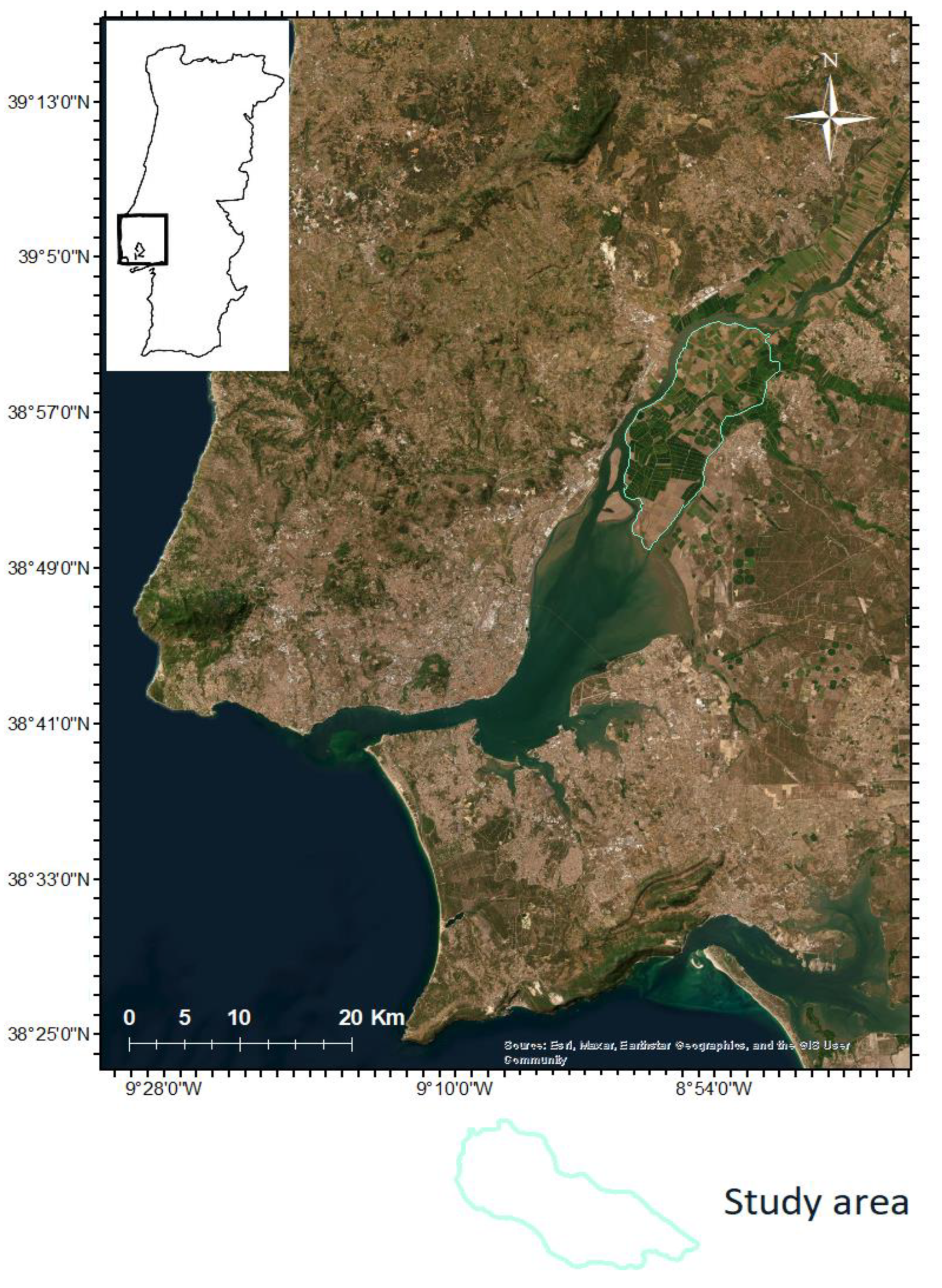
Figure 2.
Main land uses (2022) and location of the fields (A, B, C, and D) and sampling points.
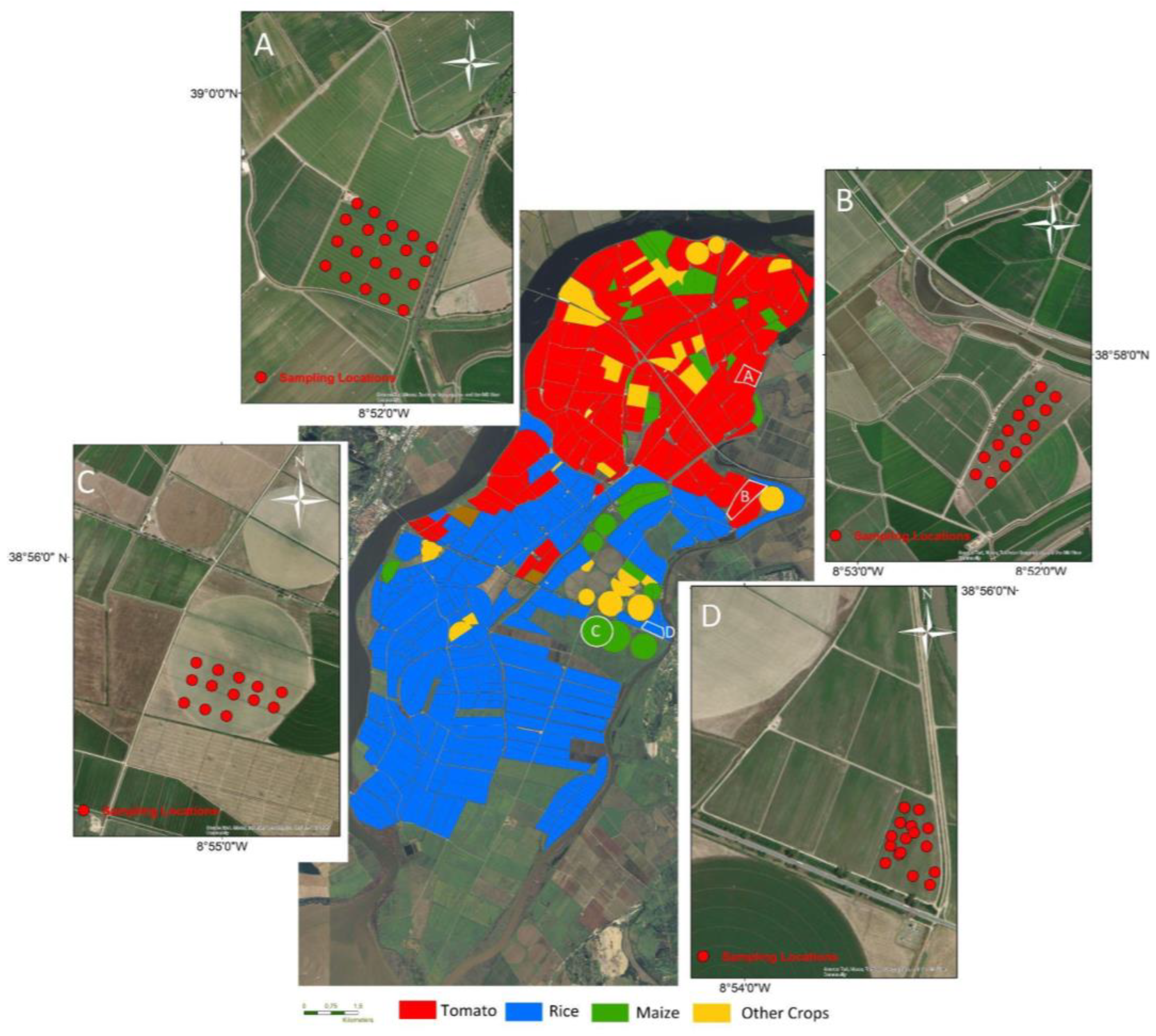
Figure 3.
a) The number of Level 2A images acquired across the study area with cloud cover of less than 10%, within the one year spanning from June 1, 2022, to June 1, 2023; b) The number of bare soil conditions per pixel during the same period.
Figure 3.
a) The number of Level 2A images acquired across the study area with cloud cover of less than 10%, within the one year spanning from June 1, 2022, to June 1, 2023; b) The number of bare soil conditions per pixel during the same period.
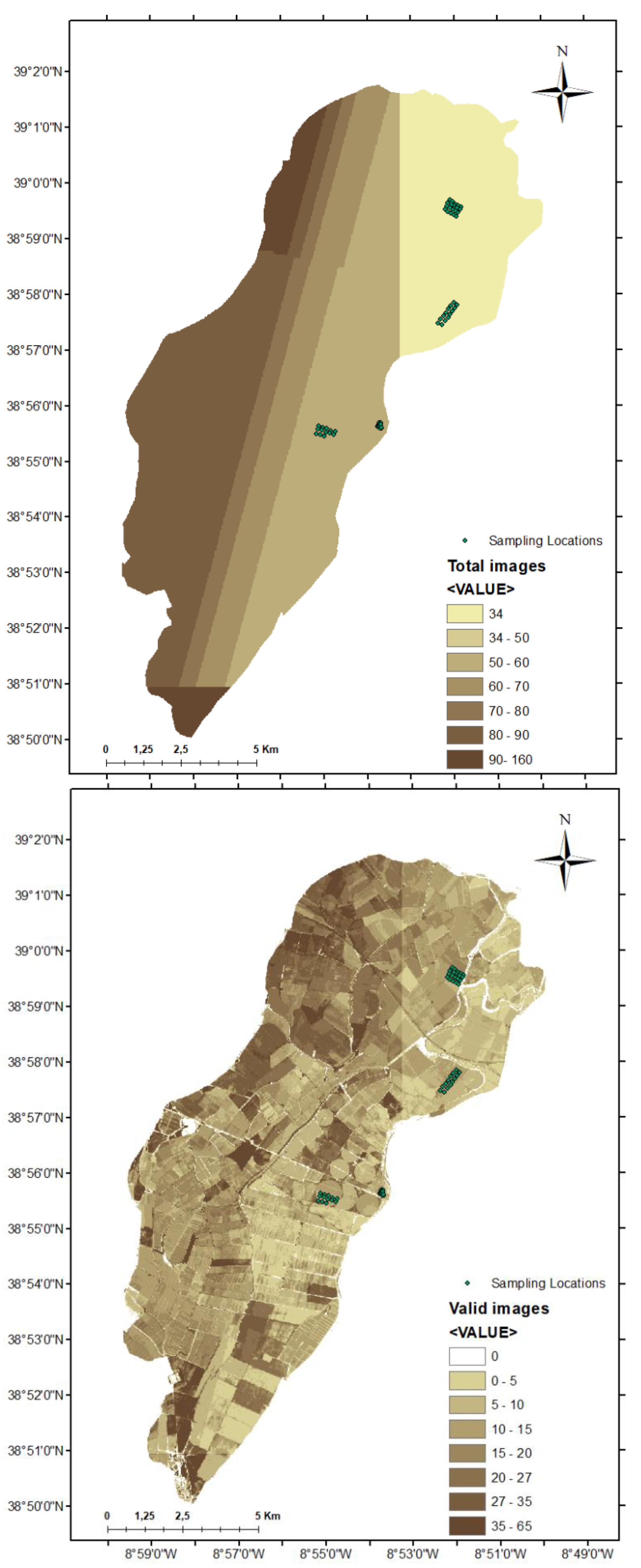
Figure 4.
Spearman correlation coefficients (significant at p< 0.01) between measured soil properties of the ground-truth dataset.
Figure 4.
Spearman correlation coefficients (significant at p< 0.01) between measured soil properties of the ground-truth dataset.
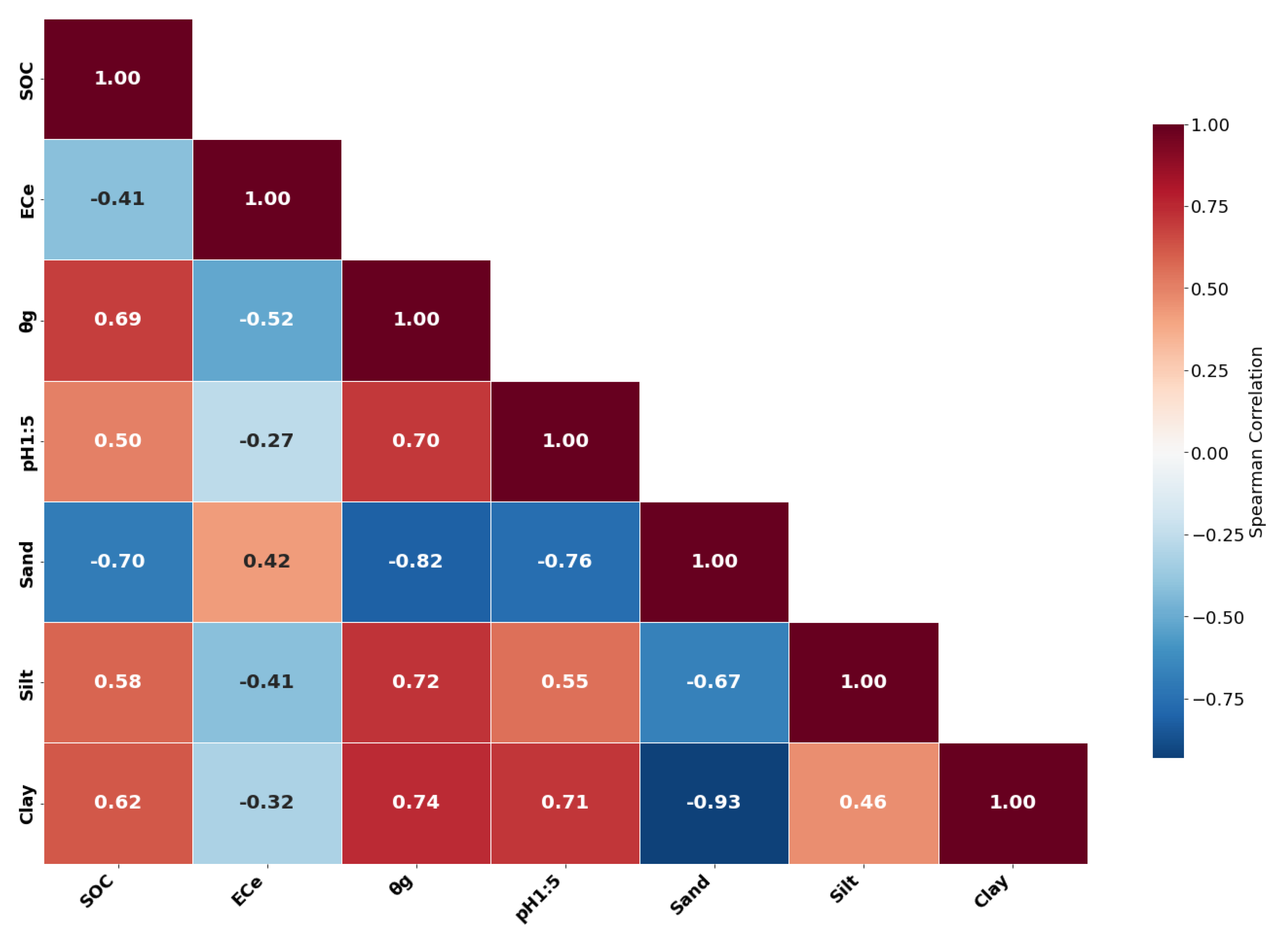
Figure 5.
Map of the maxBSI index of the study area. The 63 sampling locations are marked by green points.
Figure 5.
Map of the maxBSI index of the study area. The 63 sampling locations are marked by green points.
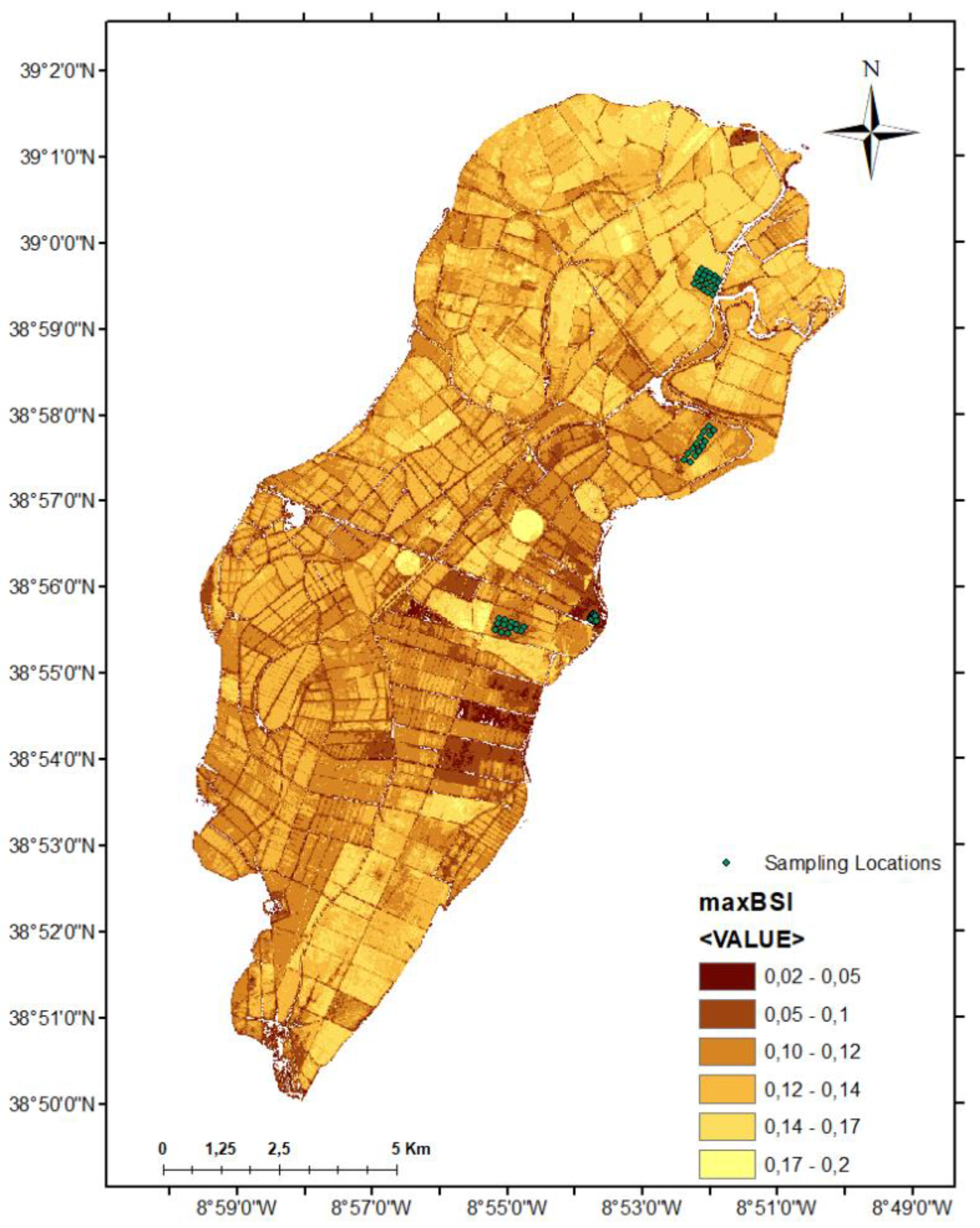
Figure 6.
Plots of a) the maxBSI and the measured SOC content [%] and the linear regression (LR) of the regional calibration equation and b) validation results of the regional LR calibration equation calculated for all four locations (shown in 6a).
Figure 6.
Plots of a) the maxBSI and the measured SOC content [%] and the linear regression (LR) of the regional calibration equation and b) validation results of the regional LR calibration equation calculated for all four locations (shown in 6a).
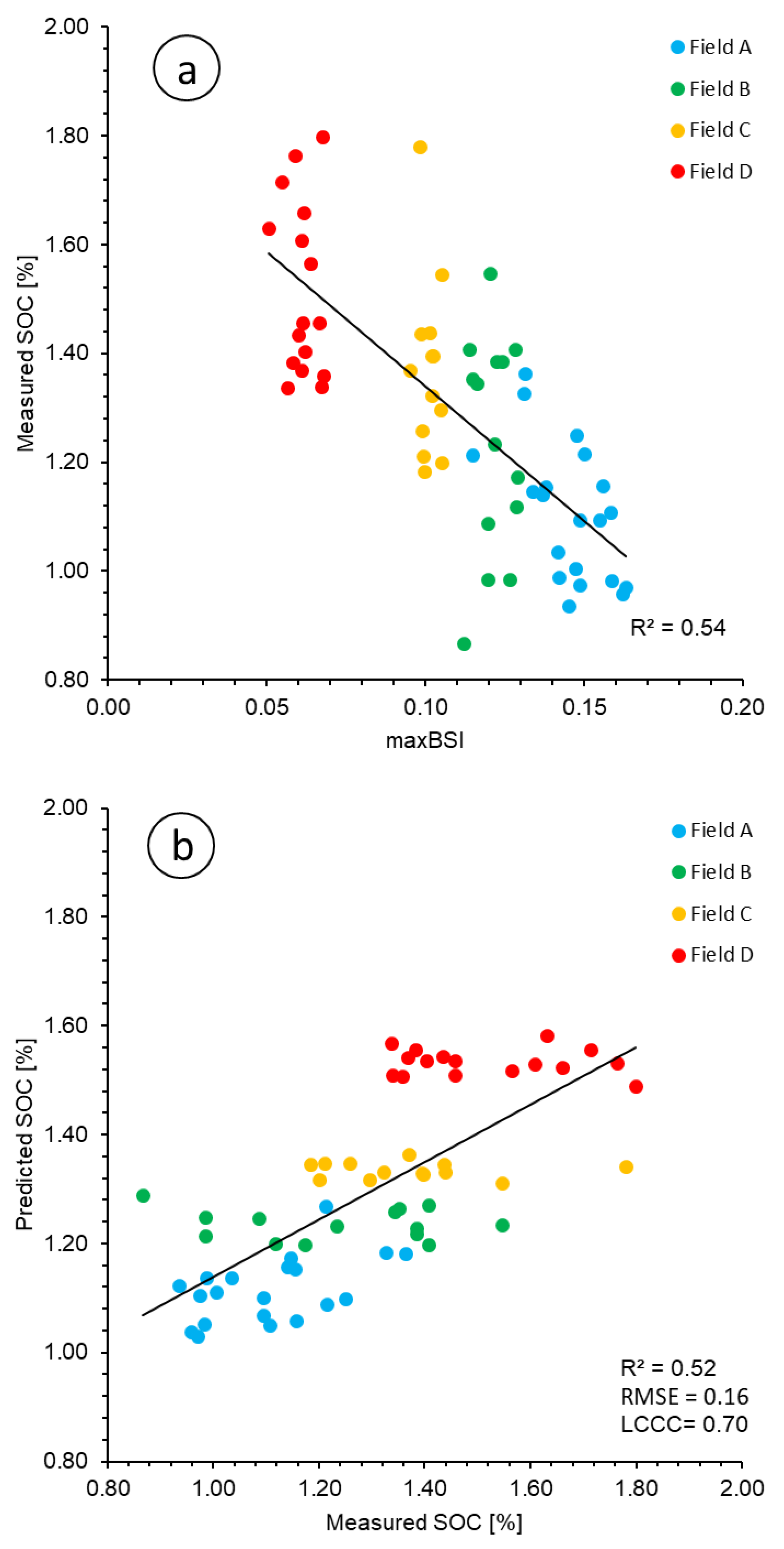
Figure 7.
Map of the predicted SOC content of the study area. The sampling locations were marked by green points.
Figure 7.
Map of the predicted SOC content of the study area. The sampling locations were marked by green points.
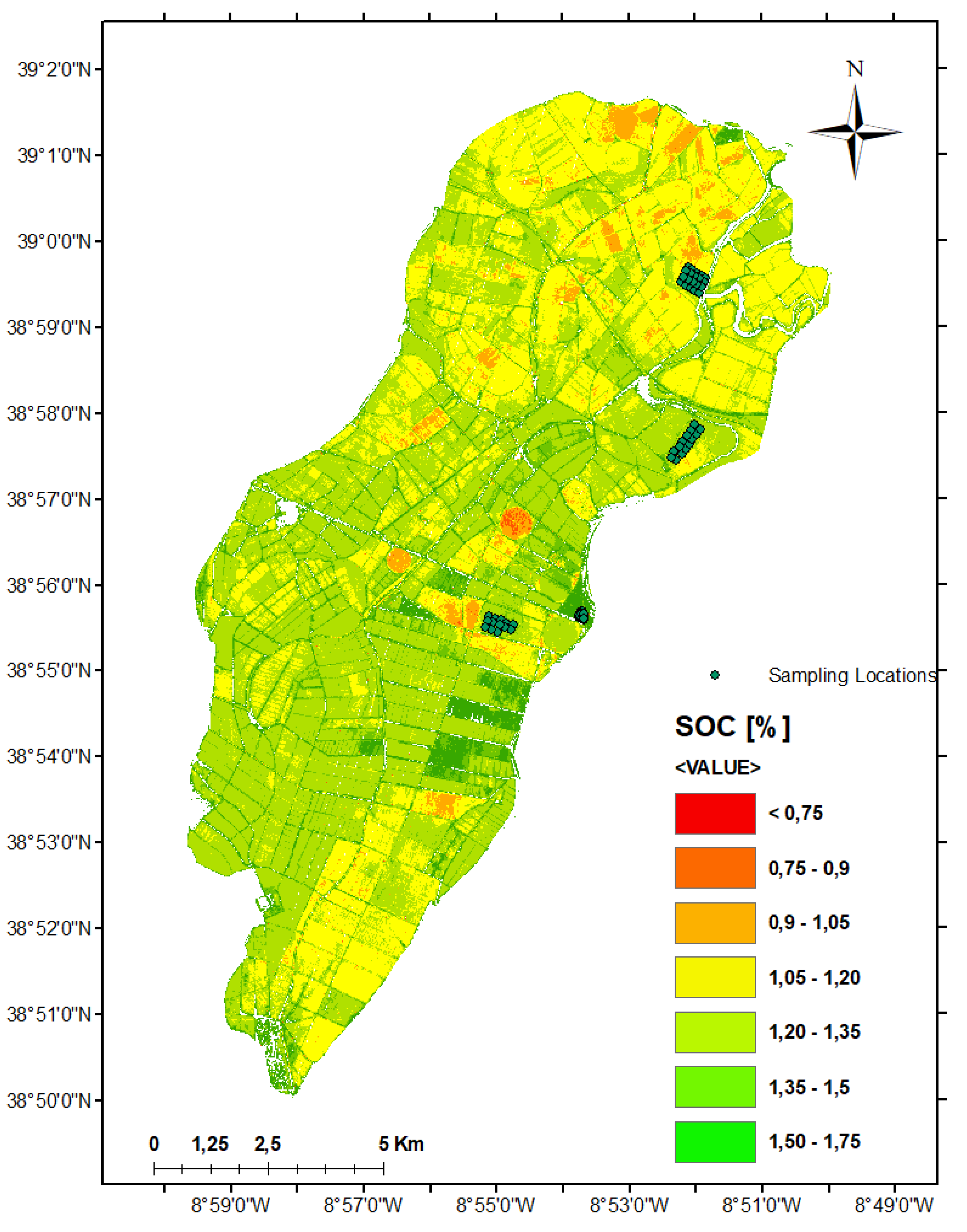
Figure 8.
Uncertainty map of the predicted SOC content expressed as prediction interval ratio (PIR; Equation5).
Figure 8.
Uncertainty map of the predicted SOC content expressed as prediction interval ratio (PIR; Equation5).
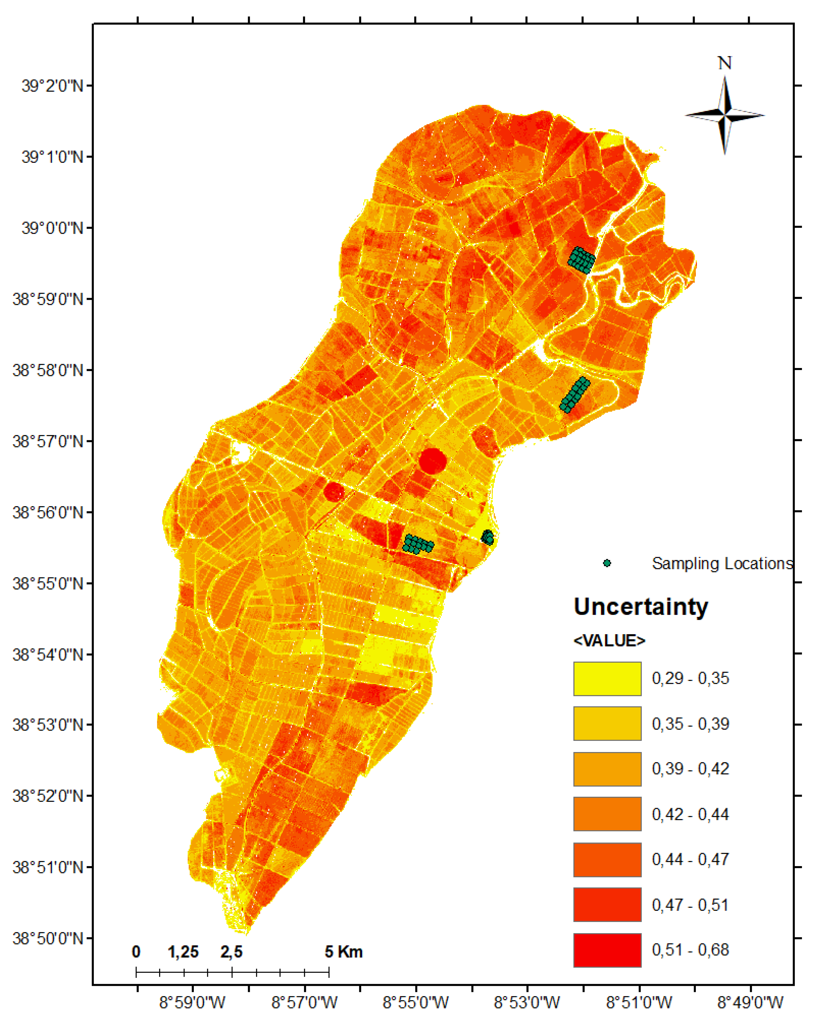
Figure 9.
Plots of the maxBSI and measured a) Clay [%], b) θg [%], c) Sand [%], d) ECe (dS m-1), and e) pH at all four locations.
Figure 9.
Plots of the maxBSI and measured a) Clay [%], b) θg [%], c) Sand [%], d) ECe (dS m-1), and e) pH at all four locations.
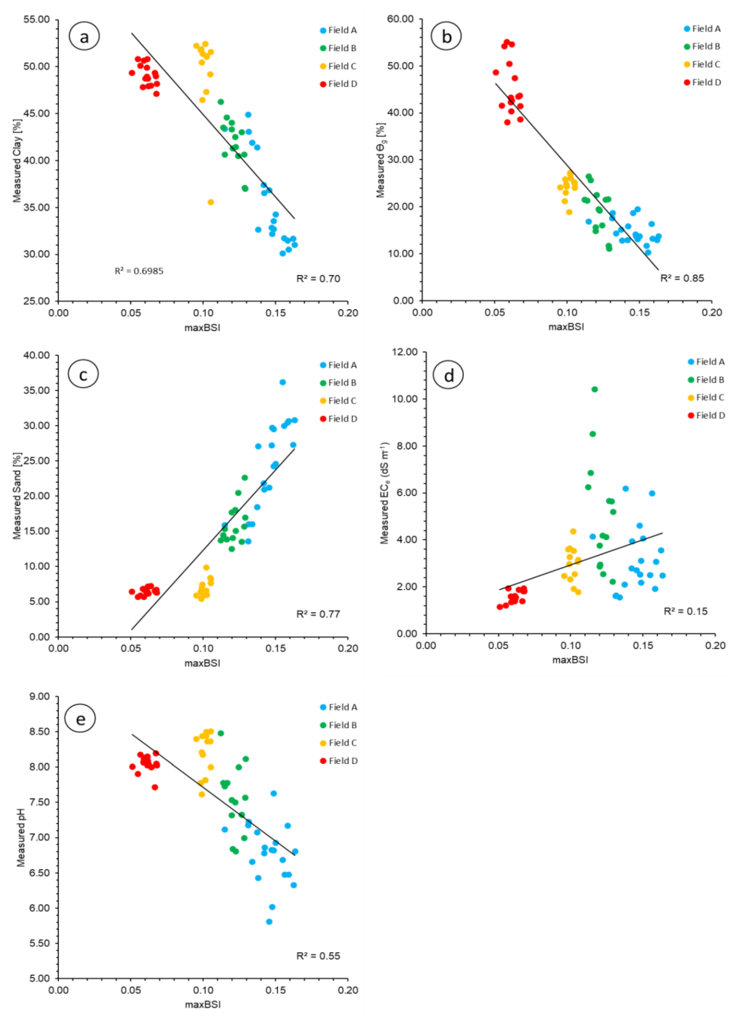

Table 1.
Features of the spectral bands used in this study.
| Spectral Band | Spatial Resolution (m) | Central Wavelength (nm) | Band Width (nm) |
|---|---|---|---|
| B2 (Blue- B) | 10 | 490 | 65 |
| B3 (Green - G) | 10 | 560 | 35 |
| B4 (Red - R) | 10 | 665 | 30 |
| B5 (Red edge - RE1) | 20 | 705 | 15 |
| B6 (Red edge - RE2) | 20 | 740 | 15 |
| B7 (Red edge - RE3) | 20 | 783 | 20 |
| B8 (Near infrared - NIR) | 10 | 842 | 115 |
| B8A (Narrow near infrared - NIRN) | 20 | 865 | 20 |
| B11 (Short wave infrared - SWIR1) | 20 | 1610 | 90 |
| B12 (Short wave infrared - SWIR2) | 20 | 2190 | 180 |
Table 2.
Characteristics and basic statistics for soil properties for the four sampled fields.
| Field | Date of Sampling | Soil Cover | Area (km2) | Nº of Samples | SOC [%] | Clay [%] | Sand [%] | |||||||||
|---|---|---|---|---|---|---|---|---|---|---|---|---|---|---|---|---|
| Min | Max | Mean | Std | Min | Max | Mean | Std | Min | Max | Mean | Std | |||||
| A | Oct 2022 | Tomato residues | 23 | 20 | 0.9 | 1.4 | 1.2 | 0.1 | 30.1 | 44.9 | 35.5 | 4.9 | 13.6 | 36.2 | 24.6 | 6.3 |
| B | Oct 2022 | Tomato residues | 33 | 14 | 0.9 | 1.5 | 1.2 | 0.2 | 37.0 | 46.3 | 41.9 | 2.6 | 12.5 | 22.6 | 16.0 | 2.9 |
| C | Oct 2022 | Maize stubble residues | 34 | 13 | 1.2 | 1.8 | 1.4 | 0.2 | 35.6 | 52.4 | 49.4 | 4.6 | 5.4 | 9.9 | 7.0 | 1.27 |
| D | Mar 2023 | Rise stove residues | 3 | 16 | 1.3 | 1.8 | 1.5 | 0.2 | 47.1 | 50.8 | 49.1 | 1.1 | 5.7 | 7.2 | 6.5 | 0.5 |
| All | 63 | 0.9 | 1.8 | 1.3 | 0.2 | 30.1 | 52.4 | 43.2 | 7.0 | 5.4 | 36.2 | 14.5 | 8.7 | |||
| Field | Date of sampling | Soil cover | Area (km2) | Nº of samples | θg [%] | Ece [dSm-1] | pH 1:5 | |||||||||
| Min | Max | Mean | Std | Min | Max | Mean | Std | Min | Max | Mean | Std | |||||
| A | Oct 2022 | Tomato residues | 23 | 20 | 10.3 | 19.5 | 14.8 | 2.5 | 1.6 | 6.2 | 3.1 | 1.3 | 5.8 | 7.6 | 6.8 | 0.4 |
| B | Oct 2022 | Tomato residues | 33 | 14 | 11.1 | 26.5 | 19.2 | 4.7 | 2.2 | 10.4 | 5.1 | 2.4 | 6.8 | 8.5 | 7.6 | 0.5 |
| C | Oct 2022 | Maize stubble residues | 34 | 13 | 19.0 | 27.3 | 24.4 | 2.3 | 1.8 | 4.4 | 3.0 | 0.7 | 7.6 | 8.5 | 8.2 | 0.3 |
| D | Mar 2023 | Rise stove residues | 3 | 16 | 38.0 | 55.1 | 45.4 | 5.7 | 1.2 | 1.9 | 1.6 | 0.2 | 7.7 | 8.2 | 8.1 | 0.1 |
| All | 63 | 10.3 | 55.1 | 25.5 | 12.8 | 1.2 | 10.4 | 3.1 | 1.8 | 5.8 | 8.5 | 7.7 | 0.7 |
Disclaimer/Publisher’s Note: The statements, opinions and data contained in all publications are solely those of the individual author(s) and contributor(s) and not of MDPI and/or the editor(s). MDPI and/or the editor(s) disclaim responsibility for any injury to people or property resulting from any ideas, methods, instructions or products referred to in the content. |
© 2025 by the authors. Licensee MDPI, Basel, Switzerland. This article is an open access article distributed under the terms and conditions of the Creative Commons Attribution (CC BY) license (http://creativecommons.org/licenses/by/4.0/).
Copyright: This open access article is published under a Creative Commons CC BY 4.0 license, which permit the free download, distribution, and reuse, provided that the author and preprint are cited in any reuse.


