Submitted:
17 April 2024
Posted:
18 April 2024
You are already at the latest version
Abstract
Soil organic matter (SOM) is important for the global carbon cycle, and hyperspectral remote sensing has proven a promising method for fast SOM content estimation. However, soil physical properties significantly affect the sensitivity of satellite hyperspectral imaging to SOM, leading to poor generalization ability of the estimation model. This study aims to improve the spatiotemporal transferability of the SOM prediction model by alleviating the coupling effect of soil physical properties on the spectra. Based on satellite hyperspectral images and soil physical variables, including soil moisture (SM), soil surface roughness (root mean squared height, RMSH), and soil bulk weight (SBW), a soil spectral correction strategy was established based on the information unmixing method. Two important grain-producing areas in Northeast China were selected as study areas to verify the performance and transferability of the spectral correction model and SOM content prediction model. The results showed that soil spectral corrections based on fourth-order polynomials and the XG-Boost algorithm had excellent accuracy and generalization ability, with residual predictive deviations (RPD) exceeding 1.4 in almost all bands. In addition, when the soil spectral correction strategy was adopted, the accuracy of the SOM prediction model and the generalization ability after model migration were significantly improved. The SOM prediction accuracy based on the XG-Boost corrected spectrum was the highest, with a coefficient of determination (R2) of 0.76, root mean square error (RMSE) of 5.74 g/kg, and RPD of 1.68. The prediction accuracy, R2, RMSE, and RPD of the model after migration were 0.72, 6.71 g/kg, and 1.53, respectively. Compared with the direct migration prediction of the model, adopting the soil spectral correction strategy based on fourth-order polynomials and XG-Boost reduced the RMSE of the SOM prediction results by 57.90% and 60.27%, respectively. The performance comparison highlighted the advantages of considering soil physical properties in regional-scale SOM prediction.
Keywords:
soil organic matter
; soil physical properties
; hyperspectral imagery
; spectrum correction
; model migration
1. Introduction
As the largest carbon reservoir among the terrestrial ecosystems, soil (pedosphere) constitutes the global carbon cycle with hydrosphere, atmosphere, biosphere, geosphere, and lithosphere [1]. Minor soil carbon pool changes can significantly alter atmospheric CO2 concentration, thereby affecting global carbon cycling and climate [2]. The vast majority of carbon stored in soil is organic carbon as the carbon component of organic matter [3,4,5]. Soil organic matter (SOM) is also the primary source of biological nutrients and energy in soil, and the SOM content is often used as a vital soil fertility evaluation indicator [6,7]. Therefore, precisely understanding the SOM content and spatial distribution is crucial for promoting sustainable agricultural development, enhancing soil carbon sequestration potential, and regulating global climate change [8,9].
Remote sensing is a low-cost, high-accuracy, real-time method for multi-angle, multi-temporal, and large-area earth observation [10,11,12]. At present, the ability of hyperspectral remote sensing to predict and map SOM contents has been confirmed in many studies [13,14,15]. With the rapid growth of remote sensing data and the urgent need for large-scale soil surveys, the research on remote sensing-based soil element content prediction has gradually shifted from constructing high-precision prediction models to establishing prediction models with strong spatiotemporal transferability [16,17,18]. Imaging spectra are the most important data source, and their characteristic response to soil chemical composition is an important foundation for hyperspectral remote sensing-based SOM content prediction [18,19,20]. However, imaging spectra are not affected by soil composition alone but comprehensively reflect the soil physical properties and chemical composition within the ground sample, and soil physical properties and chemical composition exert a coupling effect on the response to the spectrum [21,22,23]. Research has shown that the scattering contribution of soil physical properties, such as soil moisture (SM) and surface roughness properties (e.g., root mean squared height, RMSH), to spectral reflectance seriously affects the sensitivity of the hyperspectral data to the SOM content [24]. The near-infrared spectrum is very sensitive to a small amount of water or hydroxyl group, easily causing irregular radiation characteristics. As the SM content increases continuously until saturation, the soil reflectance decreases first and increases due to the specular reflection effect [25]. In addition, the RMSH increments enhance light scattering and transmission on the soil surface, thus decreasing the reflectivity, especially in the visible and near-infrared wavelength range [26]. Meanwhile, long-term high-intensity mechanized planting increases the soil bulk weight (SBW) of cultivated land. The concomitant changes in SM, SBW, and spectral reflectance exhibit a complex relationship. Generally, the increase in SM, SBW, and RMSH decreases the spectral reflectance, showing a coupling effect [27,28]. Noteworthy, the effect of SOM content on the soil spectrum is far weaker than that of soil physical properties [29]. Due to the satellite revisit period and soil physical condition uncertainties, the noise interference of soil physical properties on the spectrum greatly limits the accuracy and spatiotemporal transferability of the remote sensing-based SOM evaluation model, which needs to be solved urgently.
The data reliability and completeness when mapping information about the prediction target are often the keys to the generalization ability of the model [30,31]. To alleviate the influence of soil physical properties on hyperspectral data and improve the spatiotemporal transferability of the SOM content prediction model, scholars have fused hyperspectral data of long time series to reduce the sensitivity of the model to spectral differences caused by soil physical property changes [17,32,33,34]. Ge et al. attempted to introduce soil physical parameters as input variables into the element content prediction model [35]. Pan et al. established SOM content prediction models based on different SM ranges [36]. Most of these innovative improvement attempts at the macro scale have been successful, while the in-depth development and analysis of satellite hyperspectral images at the pixel scale are still lacking. Considering the reflectance difference caused by soil physical properties, Minasny et al. developed a spectral correction model based on the EOP method to eliminate the influence of SM [37]. Castaldi et al. synthesized the dry soil spectrum by calculating the statistical variability of dry and wet soil, thereby improving the model prediction accuracy [21]. Although these methods have corrected the hyperspectral data to a certain extent, they are mostly based on one physical parameter and ignore the coupling response of different soil physical properties to the spectrum. Due to the scarcity of soil physical data from satellite ground synchronization experiments, the potential of hyperspectral correction methods comprehensively considering multiple soil physical properties has not been fully explored.
Developing a soil spectral correction method alleviating the coupling effect of surface physical properties on soil pixel spectra is a long-term solution to improve the spatiotemporal transferability of the SOM prediction model. The complex interactions between the various surface physical properties and electromagnetic waves make it difficult to simulate the relationship between soil physical properties and the spectrum with physical models [28]. Therefore, this study aims to separate the physical and chemical soil information in the spectral data with data-driven methods. Studies have indicated various functional relationships between soil physical parameters (SM, RMSH, and SBW) and spectral reflectance, including logarithmic, exponential, and power exponential functions [26,38]. However, most previous studies were based on multi-spectral data, while the effect of soil physical properties on reflectance remained to be clarified based on hyperspectral data with more continuous and dense bands [39,40]. Although these functional relationships may change slightly due to differences in soil types, components, etc., they generally reflect the spectral characteristics induced by soil physical properties and are an essential basis for representing soil physical property information in the spectral data [41,42,43]. Based on this, spectral forward modeling can be carried out using soil physical properties, providing prior data for the soil spectral correction [44]. Moreover, separating the spectral information derived from soil physical and chemical properties requires spectral data only responding to soil chemical properties in the corresponding pure pixels. The dried and ground soil samples have the same uniform SM, SBW, and RMSH, and the soil spectra at this time is considered the “pure spectra “ that only reflects the soil chemical composition information [6]. To effectively decompose the soil physical and chemical information in the pixel spectrum, nonlinear parameter regression and machine learning models have been used to simulate the coupling relationship between soil physical property spectra, “pure spectra”, and pixel spectra, respectively. These two data-driven methods search for the rules between data through statistical analysis and machine learning training, respectively. In this way, the unknown data can be predicted, and the generalization ability of the soil spectral correction method can be guaranteed by the regression equation. For the SOM prediction model, the soil spectral correction redistributes the observation information of the original hyperspectral remote sensing to ensure the uniformity of the soil physical properties of all pixels, which helps improve the spatiotemporal transferability of the model [45,46,47].
This work seeks to establish a hyperspectral SOM prediction model with high spatiotemporal transferability, which can guide soil investigation and parameter prediction. The objectives of this study are: i) evaluating the impact of soil physical properties on satellite hyperspectral data and their contribution to the bias in SOM content prediction; ii) developing soil spectral correction methods alleviating the coupling impact of soil physical properties on satellite spectrum; and iii) determining the spatiotemporal transferability potential of satellite hyperspectral data for SOM retrieval based on a soil spectral correction strategy. Data-poor regions might benefit from the proposed SOM prediction model with strong spatiotemporal transferability when mapping SOM to develop appropriate policies.
2. Materials and Methods
Before establishing the SOM content prediction model with high accuracy and strong spatiotemporal transferability, a soil spectral correction method was developed to alleviate the coupling effect of surface physical properties on the soil pixel spectrum (Figure 1). Firstly, parameter estimation equations were used to establish empirical relationships between satellite hyperspectral data and the three main soil physical parameters SM, RMSH, and SBW. Three sets of simulated soil spectral data based on SM, RMSH, and SBW were obtained by correlating soil physical parameters with satellite hyperspectral images using empirical relationships. Then, a soil pixel spectral correction model was constructed based on the simulated spectrum, soil pixel spectrum, and ground spectrum using multi-order polynomials and various machine learning models to separate soil physical and chemical information in the pixel spectral data. Finally, the SOM prediction model was constructed using XG-Boost based on the original and corrected soil spectral data. Site 2 soil samples were used to evaluate the spatiotemporal transferability of the spectral correction models and SOM prediction models established with soil samples from Site 1.
2.1. Study Area
Site 1 is in the protected black soil cultivated land of Heilongjiang Province, Northeast China (131°30’-132°03’ E, 46°36’-46°49’ N), as shown in Figure 2, which has an area of 1095 km2. The area has a temperate monsoon climate, with an annual precipitation of approximately 614 mm. According to the World Reference Base for Soil Resources (WRB), the cultivated land is mainly Chernozems with a sedimentary layer under the topsoil, which has a clayey and heavy texture and poor permeability, often forming surface saucer water during precipitation periods [17]. The heavy sediment layer formed by the downward leaching of dark organic matter in the clay particles intensifies the water retention on the surface. The cultivated land surface is covered by a layer of black humus of over 10 cm. The soil has extremely high fertility and is rich in organic matter, which is suitable for crop growth [48].
Site 2 is in Changchun City, Jilin Province, Northeast China (125°24’-125°43’ E, 44°36’-44°46’ N), as shown in Figure 2, which has an area of 713 km2. Its terrain is flat, with an elevation between 189 and 237 m. Due to the influence of geographical location and atmospheric circulation, the region has a temperate continental monsoon climate, with a frost-free period of about 135 days and an average annual precipitation of about 580 mm. The region has rich river systems, relatively abundant agricultural water resources, and strong SM spatial heterogeneity. The soil in the region is mainly Phaeozems with a fertile cultivated layer, and maize and rice are the main crops [49,50]. Site 2 has significantly different soil type, surface characteristics, and other environmental factors than Site 1, which can verify the spatiotemporal transferability of the SOM content prediction model in this study.
2.2. Datasets
2.2.1. Soil Sampling and Topsoil Parameter Measurement
A total of 104 soil samples were collected from Site 1 on October 29, 2022 (Figure 2b). On April 14, 2023, 40 soil samples were collected from Site 2 (Figure 2c). Among them, 80 soil samples from Site 1 were used as the training set for the soil spectral correction model and SOM prediction model, and the remaining 24 samples were used as the validation set. Meanwhile, the 40 soil samples from Site 2 were used to test the spatiotemporal transferability of the spectral correction model and SOM prediction model. All soil samples were collected from the cultivated land portion of the study area during the “bare soil period.” First, one 3D laser scanner (Trimble TX8, maximum standard range: 120 m; Scanning speed: 1 million points per second) was installed at the midpoint of each edge of the quadrat to scan the soil surface structure (Figure 3). The sampling was conducted after the scanning to ensure the natural state of the soil surface structure within the sampled area. Next, nine subsamples were collected with a ring knife (depth 5 cm and volume 200 mL) in each 30 × 30 m quadrat. The real-time kinematic (RTK) survey technique was used to record the longitude and latitude of the quadrat midpoint.
After being transported to the laboratory, the SM and SBW of the nine subsamples in each quadrat were obtained through weighing and drying, and the average of the subsamples was calculated to represent the overall level of the quadrat. Then, the nine subsamples were mixed into one composite sample, ground, and sieved to a size of ≤ 0.2 mm for subsequent spectral measurements and SOM content testing [51]. The SOM content was determined using the potassium dichromate heating method. Soil spectral reflectance was measured with an ASD FieldSpec 4 spectrometer in the darkroom. To ensure the same SBW of each sample, soil samples were loaded in a disposable culture dish (60 mm diameter) for spectral measurements. Each soil sample was measured 10 times, and the average value was taken as the soil ground spectral data. The soil surface point cloud data from 3D laser scanning were spliced, cut, and filtered, and a 3D relative coordinate system was established (Figure 3b). After processing, the point cloud density was greater than 3 points/cm3, and the relative coordinate system accuracy of the point cloud was less than 2 mm. The Z coordinate of the point cloud data within the sample quadrat was extracted, and the standard deviation was calculated as the RMSH of the quadrat.
2.2.2. Hyperspectral Image Data Acquisition and Data Preprocessing
The Ziyuan1-02D (ZY1-02D) hyperspectral image data were acquired from the Aerospace Information Research Institute, Chinese Academy of Sciences. According to the soil sampling time of the two regions, the images generated on October 29, 2022 (Site 1) and April 14, 2023 (Site 2) were selected as data sources. All images have less than 1% cloud coverage and meet the characteristics of the “bare soil period.” The spatial resolution of the hyperspectral images is 30 m, with a total of 166 spectral channels and a spectral range of 400–2500 nm (Table 1). The sensor suffers strong noises in the wavelengths of 400 to 450 nm and 2460 to 2500 nm and is affected by atmospheric water vapor absorption in the wavelengths of 1290 to 1408 nm and 1828 to 1963 nm [52]. Therefore, the 450 to 1290 nm, 1408 to 1828 nm, and 1963 to 2460 nm bands were selected as the spectral bands in this study. The images were subjected to stripe removal, geometric correction, and atmospherical correction using Radiometric Calibration and FLAASH in the Environment for Visualizing Images 5.6 to obtain the original reflectance data. The bidirectional reflectance distribution function (BRDF) effect of the images is corrected by calculating the zenith angle and azimuth angle of the sun (and satellite). The kernel-driven BRDF model is used to normalize ZY1-02D reflectance to reduce the effect of observation geometry on reflectance [53].
2.3. Spectral Correction Strategy
The image pixel spectrum comprehensively reflects soil physical properties (e.g., SM, RMSH, and SBW) and chemical composition within the ground quadrat. Spectral correction aims to separate the reflection features attributed to the physical and chemical properties of the soil in the pixel spectral data, thus alleviating the coupling effect of soil physical properties on the spectrum. Firstly, linear, exponential, power exponential, and logarithmic parameter estimation equations were used to establish empirical relationships between satellite hyperspectral data and the three soil physical parameters SM, RMSH, and SBW on a band-by-band basis. These parameter estimation methods for fitting the relationship between soil physical properties and spectral reflectance have been verified in several studies [38,40].
By using the empirical relationships to associate soil physical parameters with satellite hyperspectral data, three sets of simulated soil spectral data based on SM, RMSH, and SBW were obtained. The soil ground spectrum measured with dried and ground soil samples is regarded as a “pure spectrum” that only reflects the soil chemical composition information [54]. Based on this, a spectral correction model was constructed, which took the pixel spectrum and three sets of soil physical parametric simulated spectrum as input and ground spectrum as training targets. Through multi-order polynomials and various machine learning algorithms, the correction relations between the pixel spectrum and the ground spectrum were established to strip the reflection information attributed to soil physical properties in the pixel spectrum. The multi-order polynomial equation is as follows:
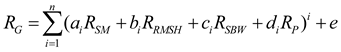 where RG is the ground-based spectral reflectance of a certain band, RSM is the spectral reflectance simulated based on SM, RRMSH is the spectral reflectance simulated based on RMSH, RSBW is the spectral reflectance simulated based on SBW, RP is the spectral reflectance of the pixel, i is the polynomial order, ai, bi, ci, di, and e are regression coefficients, respectively.
2.4. Machine Learning Models
2.4.1. Competitive Adaptive Reweighted Sampling (CARS)
CARS is adopted to extract sensitive bands corresponding to SOM in the hyperspectral data. CARS imitates the “survival of the fittest” principle of Darwin’s evolutionary theory. Through adaptive weighted sampling, it screens out the wavelengths with large absolute coefficients of the PLS model and removes the wavelengths with small weights, thus obtaining many subsets of wavelength variables. Next, the subset of wavelengths with the lowest root-mean-square error is selected via cross-validation as the optimal subset [46,55]. CARS can effectively retain the best wavelength combination related to the measured characteristics.
2.4.2. eXtreme Gradient Boosting (XG-Boost)
XG-Boost is an ensemble learning model based on the Boosting strategy, which combines several CART trees into a strong learner. As an ensemble algorithm framework, it supports the parallel gradient lifting of the base learner, thus greatly improving the model training speed. The Newton method is used to solve the extreme value of the loss function, which is expanded to the second order using the Taylor formula. The loss function is optimized with the first-order gradient function and second-order gradient function to reduce model complexity [56]. Simultaneously, the probability of over-fitting is reduced through regularization, significantly improving the model’s generalization ability.
2.4.3. Model Validation
In this study, the coefficient of determination (R2), root mean square error (RMSE), and residual predictive deviation (RPD) were selected as evaluation indices, as expressed below:
where n is the number of samples; yi and Yi represent the measured and predicted values, respectively; denotes the measurements on average.
RPD = SD/RMSE
3. Results
3.1. Description of Soil Physical Parameters and SOM Content
The statistical results of soil physical parameters and SOM content are listed in Table 2. At Site 1, the mean SM, RMSH, and SBW values were 0.25 cm3/cm3, 2.49 cm, and 0.98 g/cm3, respectively, with coefficients of variation (CV) of 31.99%, 30.92%, and 15.31%. The moderately high CV and SD indicate the combined influence of structural and anthropogenic factors on soil surface physical properties, showing strong spatial heterogeneity. The SOM content varied significantly from 25.84 to 75.97 g/kg, with a standard deviation (SD) of 10.51 g/kg and a CV of 24.30%. Site 2 had significantly different soil properties from Site 1. The average SM, RMSH, and SBW were 0.37 cm3/cm3, 3.65 cm, and 1.13 g/cm3, respectively, which were significantly higher than Site 1 and had stronger variability. The SOM content at Site 2 ranged from 27.40 to 72.97 g/kg, averaging 41.57 g/kg, which was lower than Site 1.
3.2. Effect of Soil Physical Properties on Soil Spectra
To verify the reliability of the ZY1-02D hyperspectral image, the soil pixel spectrum was compared with the soil ground spectrum (Figure 4). Although the soil pixel spectrum has a similar shape to that of the soil ground spectrum, it has some noise and a relatively low smoothness, especially in the VNIR wavelength range. In addition, the spectral reflectance in the soil pixels was slightly lower than that measured in the laboratory. The Spearman correlation coefficients (SCCs) and Pearson correlation coefficients (PCCs) between soil pixel reflectance and soil ground reflectance in each band were calculated. The results showed that the PCCs between the two sets of spectral data were below 0.5 in most wavelengths, while the SCCs in the visible light and short-wave infrared wavelength range were basically greater than 0.5, indicating a possible nonlinear relationship between the pixel spectral reflectance and the ground spectral reflectance in the same wavelength range. To further reveal the factors affecting the pixel spectrum, the differences in soil reflectance between different physical property gradients were compared. With the increase of SM, the soil spectral reflectance decreased significantly, especially in the 500 to 1300 nm and 1450 to 1700 nm wavelength ranges (Figure 5). The soil spectral reflectance decreased relatively slightly with the increase in SBW. The effect of RMSH on the soil spectrum was the most significant, and the reflectance decreased significantly with the increase of RMSH. In summary, the coupling effect of multiple soil physical properties on the spectrum is an important reason for the deviation of the two sets of spectral data, which seriously limits the acquisition of soil “pure spectrum” by the imaging spectrometer. Therefore, it is necessary to separate soil physical and chemical information in the pixel spectral data and improve the SOM prediction accuracy of hyperspectral remote sensing.
3.3. Empirical Relationship between Satellite Hyperspectral Image and Soil Physical Properties
The empirical coefficients were regressed based on the field data and soil pixel spectrum to determine the relationship of soil reflectance with SM, RMSH, and SBW (Figure 6). Among the fitting equations between SM and soil reflectance, the exponential equation has the best fitting effect. Except for the 2000 to 2500 nm wavelength range, the fitting results were good, with R2 of 0.49 to 0.68. In the 2000 to 2500 nm wavelength range, the fitting between SM and reflectance was not good, possibly due to the absorption of clay minerals to the spectral characteristics caused by the hydroxyl groups in soil. With higher clay mineral contents, the water retention capacity of the soil was greater. According to the fitting results between SBW and soil reflectance, the exponential equation fitted the best in the 450 to 1800 nm wavelength range, with the R2 of 0.50 to 0.69, while the power exponential equation fitted the best in the 2000 to 2500 nm wavelength range. In terms of the entire wavelength range, RMSH had the strongest fitting relationship with soil reflectance among the three groups of soil physical parameters, implying its most significant effect on the soil spectrum. Among the four equations, the logarithmic equation had the best fitting effect, with the R2 of 0.55 to 0.69. In general, the best empirical relationship of soil reflectance with SM is exponential, that with RMSH is logarithmic, and that with SBW is exponential in the 450 to 1800 nm wavelength range and power exponent in the 2000 to 2500 nm wavelength range. Three sets of soil reflectance data were simulated based on the empirical relationship between soil physical parameters and soil spectra, respectively (Figure 7). The soil reflectance simulated based on SM showed an almost uniform trend between 2000 and 2500 nm, implying that the effect of SM on reflectance in this wavelength range was suppressed by other factors, resulting in insignificant spectral features. Other than that, the remaining simulated soil spectra showed significant differences. These soil spectra simulated through empirical equations based on soil physical properties were used to construct the soil spectral correction model.
3.4. Modeling of Soil Spectral Correction
Empirical coefficient models and machine learning models were employed to establish the correction relationship between the soil pixel spectrum and soil “pure spectrum”. The original pixel spectrum and three sets of soil spectrum simulated based on SM, RMSH, and SBW were used as input spectral data, and the ground-based soil spectrum was used as the training target to build the soil spectral correction model band by band. The multi-order polynomial-based soil spectral correction model showed improved accuracy with the increasing order, and its RPD and RMSE were optimal in all bands at the fourth order (Figure 8). An excessively high order renders the empirical equations too complex, leading to over-fitting, reduced adaptability to new data, and decreased accuracy. The RPD of the fourth-order polynomial model was above 1.5 in all bands, indicating its good correction effect on the soil spectrum.
Four machine learning algorithms, namely, support vector machine regression (SVR), extreme learning machine (ELM), back propagation neural network (BPNN), and XG-Boost, were used to construct soil spectral correction models in the same way. The best soil spectral correction model was determined by comparing the mapping ability of the different machine learning algorithms to the coupling relationship between multiple soil spectra (Figure 9). The correction results showed that the four machine learning algorithms differed significantly in the soil spectral correction accuracy. The accuracy fluctuations around 1000 nm wavelength may be caused by other noise in the spectral data. Other than that, all soil spectral correction results were good, and the overall accuracy was high relative to the polynomial-based models. As a representative algorithm of the ensemble learning model, XG-Boost achieved the best spectral correction results, with R2 above 0.6 and RPD above 1.6 for all bands. The second best was ELM, while SVM and BPNN performed poorly.
Based on the soil spectral correction accuracy, the soil spectral correction results of the fourth-order polynomial model and XG-Boost model were selected for further analysis. The results showed that the soil spectra corrected with the XG-Boost model were smoother than those corrected with the fourth-order polynomial model and fitted the spectral shape of the soil “pure spectrum” more closely (Figure 10). The calculated correlation coefficients between the corrected soil pixel spectrum and the soil “pure spectrum” showed that the PCCs in most wavelengths were above 0.8, which was greatly improved compared with the correlation between the original pixel spectrum and the ground spectrum. Therefore, after spectral correction, the spectral response induced by soil physical properties in the soil pixel spectrum was alleviated, and the proportion of information on soil chemical composition response signals in the pixel spectral data was significantly increased. In terms of the spectral shape of the soil pixel spectral correction results and their correlation with the soil “pure spectrum,” the correction results of the XG-Boost model are slightly better than those of the fourth-order polynomial model. However, the accuracy improvement effect of these methods on hyperspectral SOM prediction needs further analysis through modeling.
3.5. SOM Content Prediction Accuracy Based on Different Spectral Data
Four types of soil spectral data, namely, pixel spectrum, fourth-order polynomial corrected spectrum, XG-Boost corrected spectrum, and ground-based spectrum, were used to establish the SOM content prediction models, respectively. In order to reduce the data dimensionality and improve the computational efficiency of the model, the spectral data were first subjected to feature extraction. Pearson’s correlation coefficient threshold was used to determine the sensitive bands of SOM. The correlation coefficient distribution between the four sets of soil spectral data and SOM content showed a relatively consistent trend. Specifically, the correlation coefficient decreased with the increasing wavelength before the 800 nm wavelength and increased after the 800 nm wavelength (Figure 11a). The bands with absolute correlation coefficients above 0.5 were selected as the sensitive bands of SOM. The sensitive spectral bands corresponding to SOM in the four spectral data sets of pixel spectrum, fourth-order polynomial corrected spectrum, XG-Boost corrected spectrum, and ground-based spectrum were concentrated in the wavelength range of 628 to 1023 nm, 524 to 1223 nm, 542 to 1560 nm, and 550 to 1762 nm, respectively. CARS was adopted to further extract the optimal subset of features containing the least redundant information in the sensitive bands. The optimal number of CARS iterations was determined by the RMSECV of multiple regression (Figure 11b). The bands listed in Table 3 are the spectral bands selected by CARS for SOM inversion modeling and validation analysis.
The four sets of spectral bands selected through CARS and the SOM contents were used as the input data of the model. The XG-Boost algorithm is used to construct the SOM prediction model. The results indicated that these two spectral correction methods significantly improved the SOM prediction accuracy based on the original pixel spectrum. Among all SOM prediction results, the ground spectral data had the highest prediction accuracy, with the , RMSEP, and RPD of 0.79, 4.89 g/kg, and 1.97, respectively (Figure 12). The prediction accuracy evaluated based on was 0.64 when the original pixel spectral dataset was used as model input data. Adopting the soil spectral correction strategy based on fourth-order polynomials increased the prediction accuracy () by 0.05, decreased RMSEP by 2.28 g/kg, and increased RPD by 0.38. The soil spectral correction strategy based on the XG-Boost model had a greater SOM prediction accuracy improvement, with an increase of 0.12, an RMSEP decrease of 3.10 g/kg, and an RPD increase of 0.59. The SOM prediction accuracy with the corrected spectrum came close to that with the ground spectrum, implying that alleviating the coupling effect of soil physical properties on the soil pixel spectrum can effectively improve the hyperspectral SOM prediction accuracy.
4. Discussion
4.1. The Transferability of the Soil Spectral Correction Model and SOM Prediction Model
The soil pixel spectral correction methods based on empirical coefficient and machine learning models provided new strategies for improving the SOM prediction accuracy based on hyperspectral images. The two soil spectral correction methods based on different models have their advantages and limitations. The soil spectral correction method based on XG-Boost significantly affected the SOM prediction accuracy improvement, but its correction process and principles were difficult to express mathematically. Despite its weak SOM prediction accuracy improvement, the soil spectral correction method based on the fourth-order polynomial model expressed the improved method with the coefficient equation, which was more conducive to its promotion. The high transferability of the soil spectral correction method is a key prerequisite for constructing a SOM prediction model with strong generalization ability [57]. To verify their spatiotemporal transferability, 40 groups of Site 2 soil pixel spectra and ground experimental data were imported into the two spectral correction models. The spectral correction results showed that the corrected soil spectra were very consistent with the shape of the soil “pure spectra” (Figure 13). Compared with the soil spectrum after fourth-order polynomial correction, the soil spectrum corrected with the XG-Boost model is smoother. According to the accuracy of the model migration test results, the soil spectral correction model based on XG-Boost showed better migration performance, with RPD above 1.4 for all bands. The machine learning algorithms represented by XG-Boost were much better than the coefficient models in terms of the calculation ability to establish the coupling relationship between multiple soil spectra and its adaptability to new data. The reason is that this ensemble learning model comprehensively utilizes all the eigenvalues of each soil sample point and continuously adjusts the weight of the tree through iteration to explore the optimal solution of the coupling relationship between soil physical properties and the pixel spectrum [45,58].
The poor spatiotemporal transferability of traditional SOM prediction models is mainly attributed to their poor applicability to different spatiotemporal spectral data [59]. Evaluating the improvement effects of soil spectral correction methods on the spatiotemporal transferability of SOM prediction models is the direct basis to prove the effectiveness of spectral correction methods [60]. The Site 2 soil samples and spectral data were used to evaluate the transferability of the SOM prediction model established with the Site 1 data. The SOM prediction model based on ground spectra exhibited the best transferability, with RMSEP only increasing by 0.39 g/kg (Figure 14). However, the transferability of SOM prediction models based on the original pixel spectrum is extremely poor as surface physical property changes cause spectral reflectance deviations. After transferability verification, RMSEP increased by 8.05 g/kg, while RDP decreased by 44.04%. Adopting the two soil spectral correction strategies significantly improved the transferability of the prediction model based on the original pixel spectrum, with an RPD of over 1.4 for model transferability validation. The SOM prediction model based on the XG-Boost correction spectrum had greater transferability. Compared with the model transferability validation based on the pixel spectrum, RMSEP was reduced by 60.27%, and RPD was increased by 150.82%. These findings proved the effectiveness of the soil spectral correction methods and the feasibility of the corrected satellite hyperspectral data to predict SOM content. The SOM prediction model based on corrected satellite hyperspectral data can be used even at two sites with different soil types, soil physical properties, SOM contents, and spatiotemporal features. The core of this soil spectral correction method is to comprehensively consider the coupling effect of various soil properties on spectral reflectance to restore the true spectral characteristics of the research target. For different research objectives, the main factors affecting the spectral response of the target can be analyzed according to the actual environment and imaging conditions [39]. Therefore, the proposed method is not limited to SOM prediction and can provide valuable insights for soil property prediction based on satellite hyperspectral data.
4.2. Contribution of Soil Physical Properties to SOM Content Prediction Bias
The soil spectral correction method proved to greatly improve the SOM content prediction accuracy and spatiotemporal transferability of the pixel spectrum. In other words, soil properties (SM, RMSH, and SBW) may be the main factors leading to errors in SOM estimation based on original pixel spectra. This section investigated the error dependence of the original pixel spectrum and two sets of corrected spectral data on SM, RMSH, and SBW, and their contribution to SOM content prediction bias was estimated through the stepwise regression method. The results showed that the cumulative deviation contribution rate of these three soil properties to the SOM prediction results based on the original pixel spectrum was over 70% at both sites (Figure 15). Thus, soil physical properties are the main error source of SOM prediction [53]. The contribution of SM to SOM bias was the highest, followed by RMSH and SBW. This is related to the most significant response of the pixel spectrum to SM within the sensitive wavelength of SOM and possibly the stronger spatial heterogeneity of SM compared to RMSH and SBW. The stronger spatial heterogeneity of soil physical properties leads to greater differences in the impact on pixel spectra and, thus, greater deviation in SOM prediction [10]. Adopting the spectral correction strategy significantly reduced the bias of SM, RMSH, and SBW in SOM prediction. Soil spectral correction based on XG-Boost more significantly reduced the SOM prediction bias caused by soil physical properties than the soil spectral correction based on fourth-order polynomials. This result fundamentally explains the higher prediction accuracy and stronger spatiotemporal transferability of the SOM prediction model based on the XG-Boost corrected spectrum. Despite the increased relative contribution of random errors, the total bias in terms of the accuracy of the predicted results was significantly reduced. Therefore, the spectral correction strategy did not introduce more error sources but only improved the relative contribution of other error factors to SOM prediction bias, such as hyperspectral image processing uncertainty and field data acquisition uncertainty [61,62]. Judging from the relative contribution rate of soil physical properties to SOM prediction deviation before and after spectral correction, the contribution rate of SM to SOM prediction bias decreased the most by over 10%, followed by RMSH. The spectral correction method based on polynomials and XG-Boost reduced the average relative contribution rate of RMSH at the two sites by 10% and 14.5%, respectively. Although the declined contribution rate of SBW to SOM prediction bias was the smallest, the reduction exceeded 6%. By comparing the improvement effects of different input variables on SOM prediction bias, the improvement effects of soil physical properties on SOM content prediction accuracy ranked as SM > RMSH > SBW, consistent with the order of spatial heterogeneity of these three soil physical properties and the order of sensitivity of soil spectra to them in the VNIR range. Thus, soil physical properties with strong spatial heterogeneity and sensitive spectral response should be prioritized in soil spectral correction.
4.3. The Potential and Limitations of the Soil Spectral Correction Model
As soil spectral correction methods are designed to address the coupled effects of surface physical properties on hyperspectral images, they are suitable for remote sensing image processing of various soil chemical composition predictions. Such methods suppress the sensitivity of spectral data to SM, RMSH, and SBW and reduce the possibility of SOM prediction results falling into the local optimum. Another advantage is that determining the empirical relationship of SM, RMSH, and SBW with the hyperspectral soil reflectance of ZY1-02D satellite spectra improves the generalization ability and application efficiency of the method. In addition, this study also has two potential applications. 1) It enables the application of optical and radar remote sensing combined in soil physicochemical property estimation, and 2) it provides a solution to the spatiotemporal heterogeneity of spectral data due to uncertain changes in surface physical conditions in multi-source remote sensing data fusion. Although the soil spectral correction model can restore most soil “pure spectrum” characteristics, some uncertainties may remain. The applicability of the proposed method to airborne hyperspectral sensors or other hyperspectral satellites requires evaluation with more data. In addition, this experiment only considered the influence of soil properties within 5 cm of the surface layer on the spectrum, while the spectrum may have different sensing depths for different soil properties [63]. Even though the spectrum only directly detects SM changes in shallow soil (about 0 to 2 cm), this depth also changes under different SBW and RMSH conditions [20,64]. The vertical heterogeneity of SM and SBW may be the main factor causing soil spectral correction errors. Adopting a hierarchical strategy to establish spectral correction models for soil properties at different depths or assigning different weights to soil physical properties at different depths may maximize the effectiveness of the model within the specified depth and range.
4.4. Future Work and Suggested Next Steps
This study, for the first time, used the “pure spectrum” derived from soil spectral correction considering SM, RMSH, and SBW for SOM content prediction and confirmed its excellent spatiotemporal transferability. The strategy of alleviating the influence of soil physical properties on spectral coupling may provide a paradigm for remote sensing-based soil element content prediction in the future. Soil spectral correction of the whole hyperspectral image requires real-time high-resolution soil physical parameter data at the regional scale. The strong sensitivity of synthetic aperture radar remote sensing to soil physical parameters makes it possible to obtain rich information on soil physical parameters in practical applications [65]. Future research may combine the advantages of hyperspectral imaging and radar remote sensing to improve the prediction accuracy of soil physicochemical parameters [66]. Given the type and dimension heterogeneity of optical and radar data, a new link to combine the two data was provided. Meanwhile, some interesting new directions have also emerged. Due to the difference in imaging time between radar and hyperspectral images, the corresponding surface physical properties also change, especially SM, which is highly susceptible to weather. Therefore, combining optical and radar data to eliminate the bias due to the temporal phase may be the optimal strategy to solve this problem. In addition, the perception depth of optical and radar remote sensing for soil properties needs further clarification. As radar sensors have better penetrability than optical sensors, quantifying the vertical heterogeneity of SM and SBW with radar remote sensing could be the key to further improving the soil spectral correction accuracy [67,68]. These strategies reduce errors in large-scale soil physical and chemical parameter surveys to support regional strategic arrangements for sustainable agricultural development.
5. Conclusions
This study utilized satellite and ground hyperspectral data and soil physical parameters data to construct two soil spectral correction models based on fourth-order polynomial and XG-Boost, respectively, to alleviate the coupling effect of soil physical properties on the pixel spectrum. The performance of the soil spectral correction models and their influence on the accuracy and spatiotemporal transferability of the SOM prediction model were evaluated using data from two sites. The main conclusions are as follows. (1) The soil pixel spectral reflectance is nonlinearly related to soil ground spectral reflectance. The difference in surface physical properties is the main factor for the deviation of the two spectral data. RMSH has the most significant effect on the soil pixel spectrum, followed by SM and SBW. (2) The fourth-order polynomial and XG-Boost models have good soil spectral correction accuracy. The soil spectral correction model based on XG-Boost has higher accuracy and stronger spatiotemporal transferability as it considers all the features to continuously adjust the weight of the tree and prevent the result from falling into the local optimum. (3) Soil spectral correction significantly alleviates the coupling effect of soil physical properties on soil pixel spectra, effectively improves the accuracy of the SOM prediction model, and, more importantly, greatly enhances the spatiotemporal transferability of the SOM prediction model based on pixel spectrum. Considering the response of satellite hyperspectral imaging to soil physical properties helps to understand their roles in SOM content prediction. This work provides a new research paradigm for predicting soil property parameters in other regions.
Author Contributions
Conceptualization, N.L. and Y.S.; methodology, R.J.; software, H.Y.; validation, X.Z.; formal analysis, R.J.; investigation, N.L. and R.J.; resources, R.J.; data curation, N.L., J.L. and X.Z.; writing—original draft preparation, R.J. and Y.S.; writing—review and editing, R.J. and Y.S.; visualization, N.L. and Y.S.; supervision, R.J.; project administration, R.J.; funding acquisition, N.L., H.Y., and X.Z. All authors have read and agreed to the published version of the manuscript.
Funding
The work was supported by the Jilin Provincial Scientific and Technological Development Program [20230101373JC and 20240303035NC]; the 14th Five-Year National Key Research and Development Plan of China [2022YFD1500504]; and the Common Application Support Platform for Land Observation Satellites of China’s Civil Space Infrastructure Project, China [CASPLOS-CCSI].
Data Availability Statement
The data presented in this study are available on request from the corresponding author.
Conflicts of Interest
The authors declare no conflict of interest.
References
- Lehmann, J.; Kleber, M. The contentious nature of soil organic matter. Nature 2015, 528, 60–68. [Google Scholar] [CrossRef] [PubMed]
- Crowther, T.W.; van den Hoogen, J.; Wan, J.; Mayes, M.A.; Keiser, A.D.; Mo, L.; Averill, C.; Maynard, D.S. The global soil community and its influence on biogeochemistry. Science 2019, 365, 772. [Google Scholar] [CrossRef] [PubMed]
- Zhou, T.; Geng, Y.; Chen, J.; Liu, M.; Haase, D.; Lausch, A. Mapping soil organic carbon content using multi-source remote sensing variables in the Heihe River Basin in China. Ecol. Indic. 2020, 114. [Google Scholar] [CrossRef]
- Zhong, L.; Chu, X.; Qian, J.; Li, J.; Sun, Z. Multi-Scale Stereoscopic Hyperspectral Remote Sensing Estimation of Heavy Metal Contamination in Wheat Soil over a Large Area of Farmland. Agronomy-Basel 2023, 13. [Google Scholar] [CrossRef]
- Wu, J.; Jin, S.; Zhu, G.; Guo, J. Monitoring of Cropland Abandonment Based on Long Time Series Remote Sensing Data: A Case Study of Fujian Province, China. Agronomy-Basel 2023, 13. [Google Scholar] [CrossRef]
- Hong, Y.; Chen, S.; Chen, Y.; Linderman, M.; Mouazen, A.M.; Liu, Y.; Guo, L.; Yu, L.; Liu, Y.; Cheng, H.; et al. Comparing laboratory and airborne hyperspectral data for the estimation and mapping of topsoil organic carbon: Feature selection coupled with random forest. Soil Tillage Res. 2020, 199. [Google Scholar] [CrossRef]
- Jiang, G.; Grafton, M.; Pearson, D.; Bretherton, M.; Holmes, A. Integration of Precision Farming Data and Spatial Statistical Modelling to Interpret Field-Scale Maize Productivity. Agriculture-Basel 2019, 9. [Google Scholar] [CrossRef]
- Schuster, J.; Hagn, L.; Mittermayer, M.; Maidl, F.-X.; Huelsbergen, K.-J. Using Remote and Proximal Sensing in Organic Agriculture to Assess Yield and Environmental Performance. Agronomy-Basel 2023, 13. [Google Scholar] [CrossRef]
- Rahmani, S.R.; Ackerson, J.P.; Schulze, D.; Adhikari, K.; Libohova, Z. Digital Mapping of Soil Organic Matter and Cation Exchange Capacity in a Low Relief Landscape Using LiDAR Data. Agronomy-Basel 2022, 12. [Google Scholar] [CrossRef]
- Wang, S.; Guan, K.; Zhang, C.; Lee, D.; Margenot, A.J.; Ge, Y.; Peng, J.; Zhou, W.; Zhou, Q.; Huang, Y. Using soil library hyperspectral reflectance and machine learning to predict soil organic carbon: Assessing potential of airborne and spaceborne optical soil sensing. Remote Sens. Environ. 2022, 271. [Google Scholar] [CrossRef]
- Angelopoulou, T.; Tziolas, N.; Balafoutis, A.; Zalidis, G.; Bochtis, D. Remote Sensing Techniques for Soil Organic Carbon Estimation: A Review. Remote Sens. 2019, 11. [Google Scholar] [CrossRef]
- Li, T.; Mu, T.; Liu, G.; Yang, X.; Zhu, G.; Shang, C. A Method of Soil Moisture Content Estimation at Various Soil Organic Matter Conditions Based on Soil Reflectance. Remote Sens. 2022, 14. [Google Scholar] [CrossRef]
- Zhan, D.; Mu, Y.; Duan, W.; Ye, M.; Song, Y.; Song, Z.; Yao, K.; Sun, D.; Ding, Z. Spatial Prediction and Mapping of Soil Water Content by TPE-GBDT Model in Chinese Coastal Delta Farmland with Sentinel-2 Remote Sensing Data. Agriculture-Basel 2023, 13. [Google Scholar] [CrossRef]
- Wang, L.; Zhou, Y. Combining Multitemporal Sentinel-2A Spectral Imaging and Random Forest to Improve the Accuracy of Soil Organic Matter Estimates in the Plough Layer for Cultivated Land. Agriculture-Basel 2023, 13. [Google Scholar] [CrossRef]
- Suleymanov, A.; Gabbasova, I.; Komissarov, M.; Suleymanov, R.; Garipov, T.; Tuktarova, I.; Belan, L. Random Forest Modeling of Soil Properties in Saline Semi-Arid Areas. Agriculture-Basel 2023, 13. [Google Scholar] [CrossRef]
- Yang, Y.; Shang, K.; Xiao, C.; Wang, C.; Tang, H. Spectral Index for Mapping Topsoil Organic Matter Content Based on ZY1-02D Satellite Hyperspectral Data in Jiangsu Province, China. ISPRS Int. J. Geo-Inf. 2022, 11. [Google Scholar] [CrossRef]
- Meng, X.; Bao, Y.; Wang, Y.; Zhang, X.; Liu, H. An advanced soil organic carbon content prediction model via fused temporal-spatial-spectral (TSS) information based on machine learning and deep learning algorithms. Remote Sens. Environ. 2022, 280. [Google Scholar] [CrossRef]
- Luo, C.; Zhang, W.; Zhang, X.; Liu, H. Mapping of soil organic matter in a typical black soil area using Landsat-8 synthetic images at different time periods. Catena 2023, 231. [Google Scholar] [CrossRef]
- Luo, C.; Wang, Y.; Zhang, X.; Zhang, W.; Liu, H. Spatial prediction of soil organic matter content using multiyear synthetic images and partitioning algorithms. Catena 2022, 211. [Google Scholar] [CrossRef]
- Croft, H.; Anderson, K.; Kuhn, N.J. Evaluating the influence of surface soil moisture and soil surface roughness on optical directional reflectance factors. Eur. J. Soil Sci. 2014, 65, 605–612. [Google Scholar] [CrossRef]
- Castaldi, F.; Palombo, A.; Pascucci, S.; Pignatti, S.; Santini, F.; Casa, R. Reducing the Influence of Soil Moisture on the Estimation of Clay from Hyperspectral Data: A Case Study Using Simulated PRISMA Data. Remote Sens. 2015, 7, 15561–15582. [Google Scholar] [CrossRef]
- Prudnikova, E.; Savin, I. Some Peculiarities of Arable Soil Organic Matter Detection Using Optical Remote Sensing Data. Remote Sens. 2021, 13. [Google Scholar] [CrossRef]
- Wang, S.; Gao, J.; Zhuang, Q.; Lu, Y.; Gu, H.; Jin, X. Multispectral Remote Sensing Data Are Effective and Robust in Mapping Regional Forest Soil Organic Carbon Stocks in a Northeast Forest Region in China. Remote Sens. 2020, 12. [Google Scholar] [CrossRef]
- Castaldi, F.; Hueni, A.; Chabrillat, S.; Ward, K.; Buttafuoco, G.; Bomans, B.; Vreys, K.; Brell, M.; van Wesemael, B. Evaluating the capability of the Sentinel 2 data for soil organic carbon prediction in croplands. ISPRS-J. Photogramm. Remote Sens. 2019, 147, 267–282. [Google Scholar] [CrossRef]
- Rienzi, E.A.; Mijatovic, B.; Mueller, T.G.; Matocha, C.J.; Sikora, F.J.; Castrignano, A. Prediction of Soil Organic Carbon under Varying Moisture Levels using Reflectance Spectroscopy. Soil Sci. Soc. Am. J. 2014, 78, 958–967. [Google Scholar] [CrossRef]
- Zhang, Y.; Zhou, L.; Zhou, Y.; Zhang, L.; Yao, X.; Shi, K.; Jeppesen, E.; Yu, Q.; Zhu, W. Chromophoric dissolved organic matter in inland waters: Present knowledge and future challenges. Sci. Total Environ. 2021, 759. [Google Scholar] [CrossRef] [PubMed]
- Yue, J.; Tian, Q.; Tang, S.; Xu, K.; Zhou, C. A dynamic soil endmember spectrum selection approach for soil and crop residue linear spectral unmixing analysis. Int. J. Appl. Earth Obs. Geoinf. 2019, 78, 306–317. [Google Scholar] [CrossRef]
- Ou, D.; Tan, K.; Li, J.; Wu, Z.; Zhao, L.; Ding, J.; Wang, X.; Zou, B. Prediction of soil organic matter by Kubelka-Munk based airborne hyperspectral moisture removal model. Int. J. Appl. Earth Obs. Geoinf. 2023, 124. [Google Scholar] [CrossRef]
- Lin, C.; Zhu, A.X.; Wang, Z.; Wang, X.; Ma, R. The refined spatiotemporal representation of soil organic matter based on remote images fusion of Sentinel-2 and Sentinel-3. Int. J. Appl. Earth Obs. Geoinf. 2020, 89. [Google Scholar] [CrossRef]
- Gholizadeh, A.; Zizala, D.; Saberioon, M.; Boruvka, L. Soil organic carbon and texture retrieving and mapping using proximal, airborne and Sentinel-2 spectral imaging. Remote Sens. Environ. 2018, 218, 89–103. [Google Scholar] [CrossRef]
- Fiorentini, M.; Zenobi, S.; Orsini, R. Remote and Proximal Sensing Applications for Durum Wheat Nutritional Status Detection in Mediterranean Area. Agriculture-Basel 2021, 11. [Google Scholar] [CrossRef]
- Abdelsamie, E.A.; Abdellatif, M.A.; Hassan, F.O.; El Baroudy, A.A.; Mohamed, E.S.; Kucher, D.E.; Shokr, M.S. Integration of RUSLE Model, Remote Sensing and GIS Techniques for Assessing Soil Erosion Hazards in Arid Zones. Agriculture-Basel 2023, 13. [Google Scholar] [CrossRef]
- Mendes, W.d.S.; Sommer, M. Advancing Soil Organic Carbon and Total Nitrogen Modelling in Peatlands: The Impact of Environmental Variable Resolution and vis-NIR Spectroscopy Integration. Agronomy-Basel 2023, 13. [Google Scholar] [CrossRef]
- Fathizad, H.; Taghizadeh-Mehrjardi, R.; Ardakani, M.A.H.; Zeraatpisheh, M.; Heung, B.; Scholten, T. Spatiotemporal Assessment of Soil Organic Carbon Change Using Machine-Learning in Arid Regions. Agronomy-Basel 2022, 12. [Google Scholar] [CrossRef]
- Ge, X.; Ding, J.; Teng, D.; Wang, J.; Huo, T.; Jin, X.; Wang, J.; He, B.; Han, L. Updated soil salinity with fine spatial resolution and high accuracy: The synergy of Sentinel-2 MSI, environmental covariates and hybrid machine learning approaches. Catena 2022, 212. [Google Scholar] [CrossRef]
- Pan, Y.; Zhang, X.; Liu, H.; Wu, D.; Dou, X.; Xu, M.; Jiang, Y. Remote sensing inversion of soil organic matter by using the subregion method at the field scale. Precis. Agric. 2022, 23, 1813–1835. [Google Scholar] [CrossRef]
- Minasny, B.; McBratney, A.B.; Bellon-Maurel, V.; Roger, J.-M.; Gobrecht, A.; Ferrand, L.; Joalland, S. Removing the effect of soil moisture from NIR diffuse reflectance spectra for the prediction of soil organic carbon. Geoderma 2011, 167-68, 118–124. [Google Scholar] [CrossRef]
- Chen, S.; Zhao, K.; Jiang, T.; Li, X.; Zheng, X.; Wan, X.; Zhao, X. Predicting Surface Roughness and Moisture of Bare Soils Using Multiband Spectral Reflectance Under Field Conditions. Chin. Geogr. Sci. 2018, 28, 986–997. [Google Scholar] [CrossRef]
- Palmisano, D.; Satalino, G.; Balenzano, A.; Mattia, F. Coherent and Incoherent Change Detection for Soil Moisture Retrieval From Sentinel-1 Data. IEEE Geosci. Remote Sens. Lett. 2022, 19. [Google Scholar] [CrossRef]
- Chen, K.S.; Wu, T.D.; Tsang, L.; Li, Q.; Shi, J.C.; Fung, A.K. Emission of rough surfaces calculated by the integral equation method with comparison to three-dimensional moment method Simulations. IEEE Trans. Geosci. Remote Sensing 2003, 41, 90–101. [Google Scholar] [CrossRef]
- Yuan, J.; Wang, X.; Yan, C.-x.; Wang, S.-r.; Ju, X.-p.; Li, Y. Soil Moisture Retrieval Model for Remote Sensing Using Reflected Hyperspectral Information. Remote Sens. 2019, 11. [Google Scholar] [CrossRef]
- Wang, Q.; Li, P.; Pu, Z.; Chen, X. Calibration and validation of salt-resistant hyperspectral indices for estimating soil moisture in arid land. J. Hydrol. 2011, 408, 276–285. [Google Scholar] [CrossRef]
- Jiang, C.; Fang, H. GSV: a general model for hyperspectral soil reflectance simulation. Int. J. Appl. Earth Obs. Geoinf. 2019, 83. [Google Scholar] [CrossRef]
- Chi, J.; Crawford, M.M. Spectral Unmixing-Based Crop Residue Estimation Using Hyperspectral Remote Sensing Data: A Case Study at Purdue University. IEEE J. Sel. Top. Appl. Earth Observ. Remote Sens. 2014, 7, 2531–2539. [Google Scholar] [CrossRef]
- Yang, L.; He, X.; Shen, F.; Zhou, C.; Zhu, A.X.; Gao, B.; Chen, Z.; Li, M. Improving prediction of soil organic carbon content in croplands using phenological parameters extracted from NDVI time series data. Soil Tillage Res. 2020, 196. [Google Scholar] [CrossRef]
- Xu, S.; Zhao, Y.; Wang, M.; Shi, X. Determination of rice root density from Vis-NIR spectroscopy by support vector machine regression and spectral variable selection techniques. Catena 2017, 157, 12–23. [Google Scholar] [CrossRef]
- Esteves, C.; Fangueiro, D.; Braga, R.P.; Martins, M.; Botelho, M.; Ribeiro, H. Assessing the Contribution of EC<sub>a</sub> and NDVI in the Delineation of Management Zones in a Vineyard. Agronomy-Basel 2022, 12. [Google Scholar] [CrossRef]
- Cui, M.; Cai, Q.; Zhu, A.; Fan, H. Soil erosion along a long slope in the gentle hilly areas of black soil region in Northeast China. J. Geogr. Sci. 2007, 17, 375–383. [Google Scholar] [CrossRef]
- Suleman, M.M.; Xu, H.; Zhang, W.; Nizamuddin, D.; Xu, M. Soil microbial biomass carbon and carbon dioxide response by glucose-C addition in black soil of China. Soil Environ. 2019, 38, 48–56. [Google Scholar] [CrossRef]
- Ou, Y.; Rousseau, A.N.; Wang, L.; Yan, B. Spatio-temporal patterns of soil organic carbon and pH in relation to environmental factors-A case study of the Black Soil Region of Northeastern China. Agric. Ecosyst. Environ. 2017, 245, 22–31. [Google Scholar] [CrossRef]
- Koegel-Knabner, I.; Guggenberger, G.; Kleber, M.; Kandeler, E.; Kalbitz, K.; Scheu, S.; Eusterhues, K.; Leinweber, P. Organo-mineral associations in temperate soils:: Integrating biology, mineralogy, and organic matter chemistry. J. Plant Nutr. Soil Sci. 2008, 171, 61–82. [Google Scholar] [CrossRef]
- Lin, N.; Jiang, R.; Li, G.; Yang, Q.; Li, D.; Yang, X. Estimating the heavy metal contents in farmland soil from hyperspectral images based on Stacked AdaBoost ensemble learning. Ecol. Indic. 2022, 143. [Google Scholar] [CrossRef]
- Zheng, X.; Feng, Z.; Li, L.; Li, B.; Jiang, T.; Li, X.; Li, X.; Chen, S. Simultaneously estimating surface soil moisture and roughness of bare soils by combining optical and radar data. Int. J. Appl. Earth Obs. Geoinf. 2021, 100. [Google Scholar] [CrossRef]
- Xu, Y.; Tan, Y.; Abd-Elrahman, A.; Fan, T.; Wang, Q. Incorporation of Fused Remote Sensing Imagery to Enhance Soil Organic Carbon Spatial Prediction in an Agricultural Area in Yellow River Basin, China. Remote Sens. 2023, 15. [Google Scholar] [CrossRef]
- Tan, K.; Ma, W.; Chen, L.; Wang, H.; Du, Q.; Du, P.; Yan, B.; Liu, R.; Li, H. Estimating the distribution trend of soil heavy metals in mining area from HyMap airborne hyperspectral imagery based on ensemble learning. J. Hazard. Mater. 2021, 401. [Google Scholar] [CrossRef]
- Lin, N.; Fu, J.; Jiang, R.; Li, G.; Yang, Q. Lithological Classification by Hyperspectral Images Based on a Two-Layer XGBoost Model, Combined with a Greedy Algorithm. Remote Sens. 2023, 15. [Google Scholar] [CrossRef]
- Ge, X.; Ding, J.; Teng, D.; Xie, B.; Zhang, X.; Wang, J.; Han, L.; Bao, Q.; Wang, J. Exploring the capability of Gaofen-5 hyperspectral data for assessing soil salinity risks. Int. J. Appl. Earth Obs. Geoinf. 2022, 112. [Google Scholar] [CrossRef]
- Guo, L.; Sun, X.; Fu, P.; Shi, T.; Dang, L.; Chen, Y.; Linderman, M.; Zhang, G.; Zhang, Y.; Jiang, Q.; et al. Mapping soil organic carbon stock by hyperspectral and time-series multispectral remote sensing images in low-relief agricultural areas. Geoderma 2021, 398. [Google Scholar] [CrossRef]
- Honarbakhsh, A.; Tahmoures, M.; Afzali, S.F.; Khajehzadeh, M.; Ali, M.S. Remote sensing and relief data to predict soil saturated hydraulic conductivity in a calcareous watershed, Iran. Catena 2022, 212. [Google Scholar] [CrossRef]
- Liu, S.; Chen, J.; Guo, L.; Wang, J.; Zhou, Z.; Luo, J.; Yang, R. Prediction of soil organic carbon in soil profiles based on visible-near-infrared hyperspectral imaging spectroscopy. Soil Tillage Res. 2023, 232. [Google Scholar] [CrossRef]
- Yang, R.-M.; Guo, W.-W. Modelling of soil organic carbon and bulk density in invaded coastal wetlands using Sentinel-1 imagery. Int. J. Appl. Earth Obs. Geoinf. 2019, 82. [Google Scholar] [CrossRef]
- Gao, L.; Zhu, X.; Han, Z.; Wang, L.; Zhao, G.; Jiang, Y. Spectroscopy-Based Soil Organic Matter Estimation in Brown Forest Soil Areas of the Shandong Peninsula, China. Pedosphere 2019, 29, 810–818. [Google Scholar] [CrossRef]
- Selige, T.; Boehner, J.; Schmidhalter, U. High resolution topsoil mapping using hyperspectral image and field data in multivariate regression modeling procedures. Geoderma 2006, 136, 235–244. [Google Scholar] [CrossRef]
- Krzyszczak, J.; Baranowski, P.; Pastuszka, J.; Wesolowska, M.; Cymerman, J.; Slawinski, C.; Siedliska, A. Assessment of soil water retention characteristics based on VNIR/SWIR hyperspectral imaging of soil surface. Soil Tillage Res. 2023, 233. [Google Scholar] [CrossRef]
- Eshqi Molan, Y.; Lu, Z. Modeling InSAR Phase and SAR Intensity Changes Induced by Soil Moisture. IEEE Trans. Geosci. Remote Sensing 2020, 58, 4967–4975. [Google Scholar] [CrossRef]
- Van Hateren, T.C.C.; Chini, M.; Matgen, P.; Pulvirenti, L.; Pierdicca, N.; Teuling, A.J.J. On the Use of Native Resolution Backscatter Intensity Data for Optimal Soil Moisture Retrieval. IEEE Geosci. Remote Sens. Lett. 2023, 20. [Google Scholar] [CrossRef]
- Zhang, Z.; Lin, H.; Wang, M.; Liu, X.; Chen, Q.; Wang, C.; Zhang, H. A Review of Satellite Synthetic Aperture Radar Interferometry Applications in Permafrost Regions: Current Status, Challenges, and Trends. IEEE Geosci. Remote Sens. Mag. 2022, 10, 93–114. [Google Scholar] [CrossRef]
- Shilpa, K.; Raju, C.S.; Mandal, D.; Rao, Y.S.; Shetty, A. Soil Moisture Retrieval Over Crop Fields from Multi-polarization SAR Data. J. Indian Soc. Remote Sens. 2023, 51, 949–962. [Google Scholar] [CrossRef]
Figure 1.
Flowchart of SOM content prediction from hyperspectral data in this study.
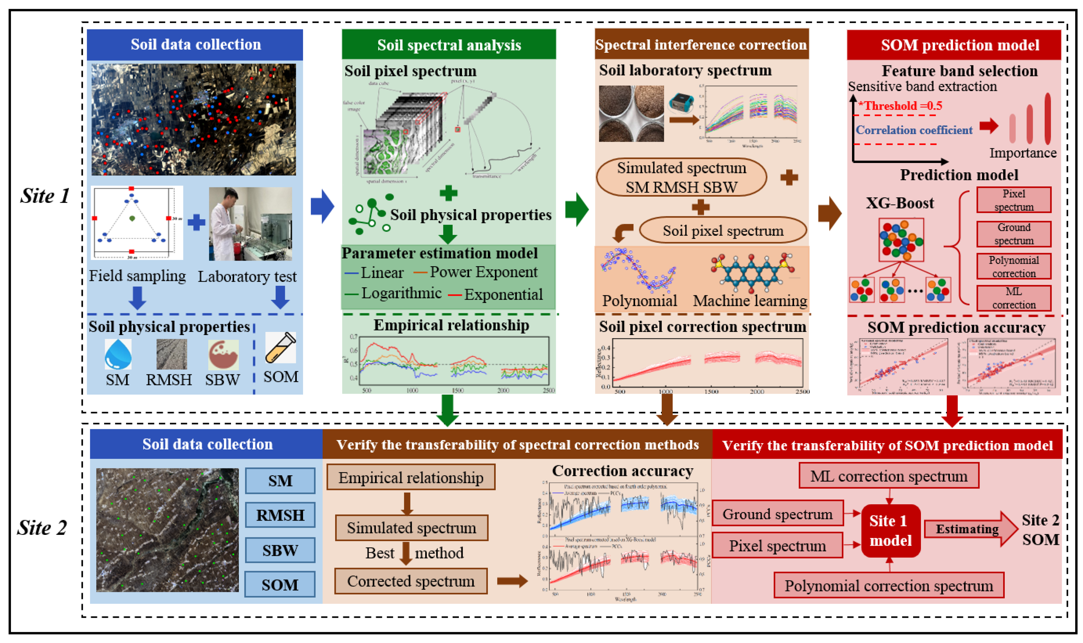
Figure 2.
Overview of study area. (a) The geographical location of the sampling sites in Heilongjiang and Jilin provinces in Northeast China; (b, c) The soil parameter measurement points and topsoil sampling points in Site 1 and Site 2, respectively; (d, e) The soil surfaces during the “bare soil period.”.
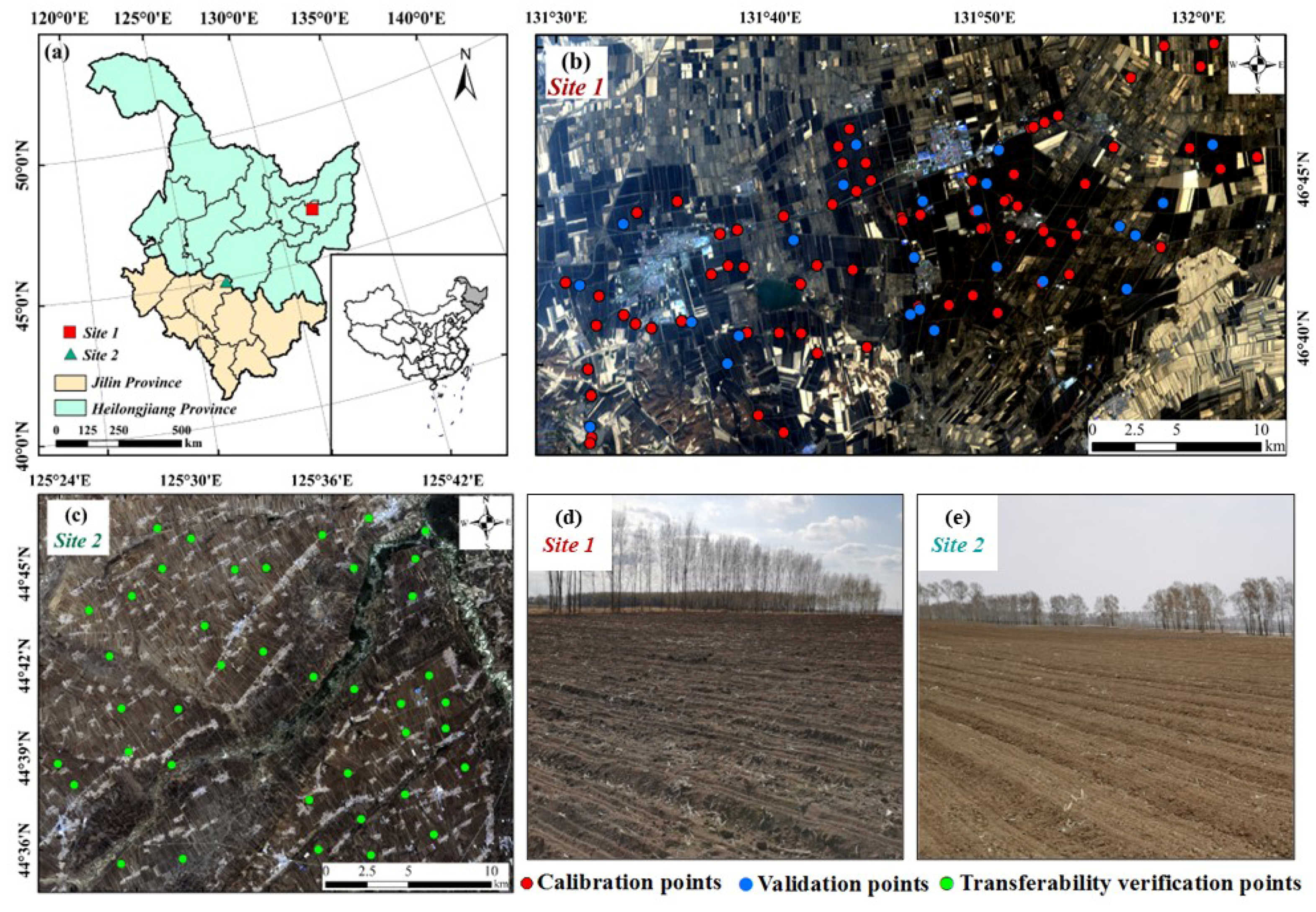
Figure 3.
Schematic diagram of soil sampling and topsoil parameter measurement. (a) Soil sampling points and 3D laser stations within a quadrat; (b) 3D laser scanning of a quadrat to generate soil surface point clouds.
Figure 3.
Schematic diagram of soil sampling and topsoil parameter measurement. (a) Soil sampling points and 3D laser stations within a quadrat; (b) 3D laser scanning of a quadrat to generate soil surface point clouds.
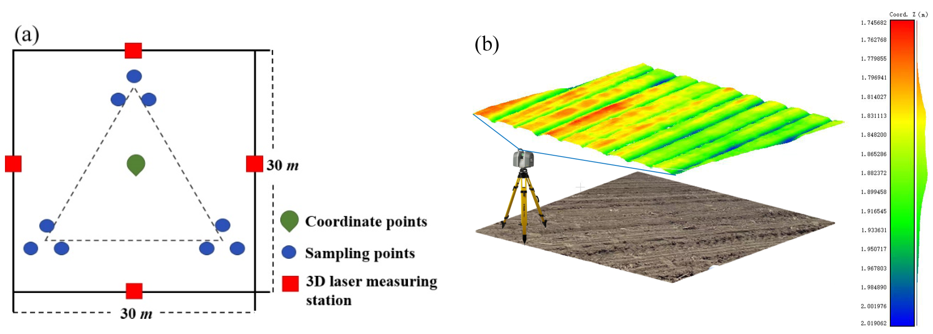
Figure 4.
Soil pixel spectrum, soil ground spectrum, and correlation coefficients of two sets of spectral reflectance.
Figure 4.
Soil pixel spectrum, soil ground spectrum, and correlation coefficients of two sets of spectral reflectance.
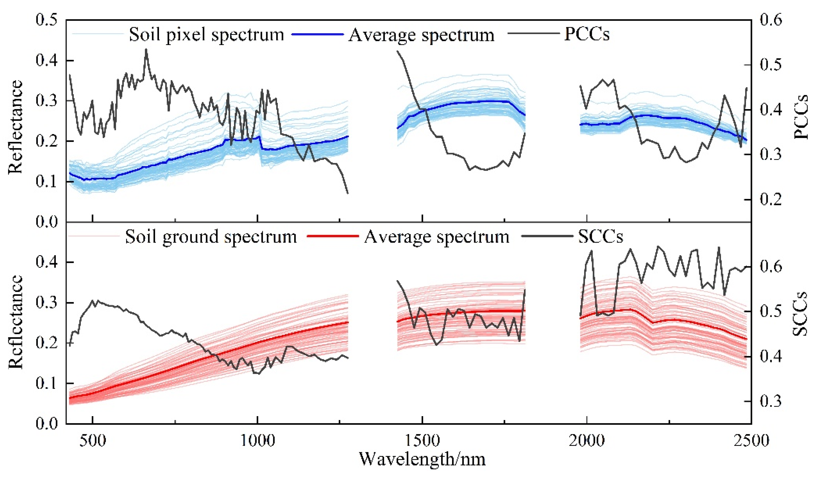
Figure 5.
Spectral characteristics of soils with different physical properties.
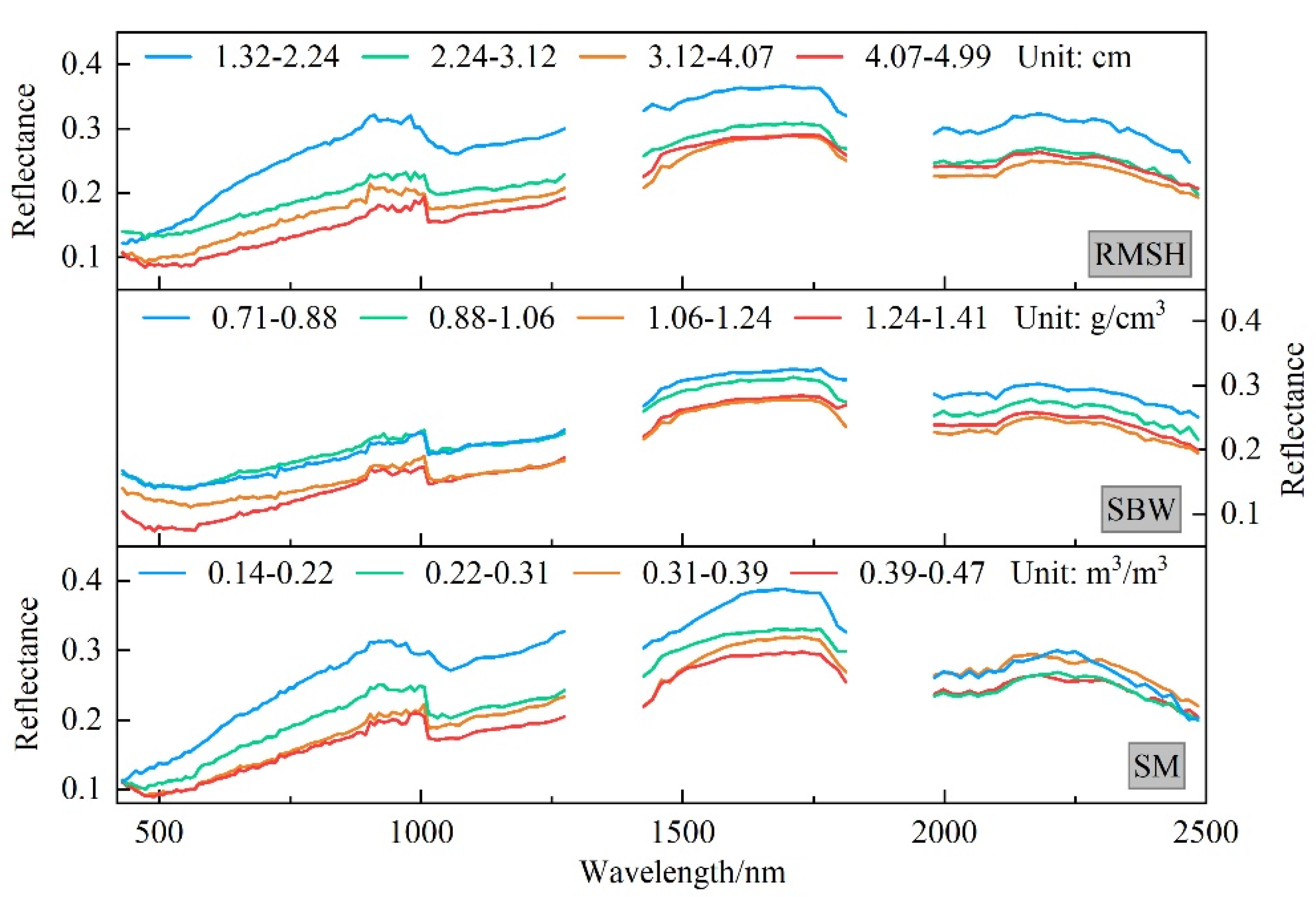
Figure 6.
R2 for fitting soil physical parameters to soil pixel spectrum based on multiple parameter estimation models.
Figure 6.
R2 for fitting soil physical parameters to soil pixel spectrum based on multiple parameter estimation models.
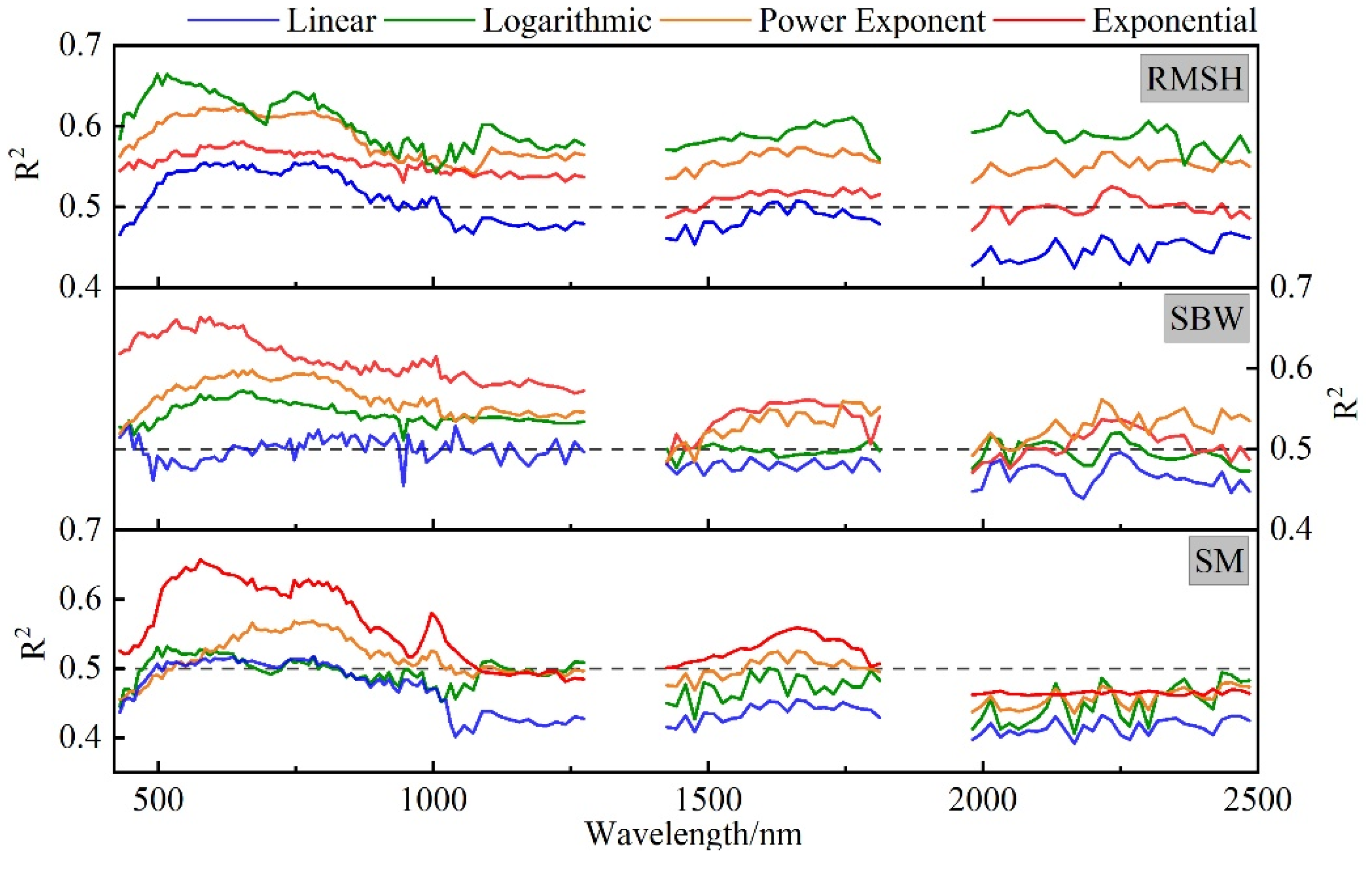
Figure 7.
Soil spectrum simulated through empirical equations based on SM (a), RMSH (b), and SBW (c).
Figure 7.
Soil spectrum simulated through empirical equations based on SM (a), RMSH (b), and SBW (c).
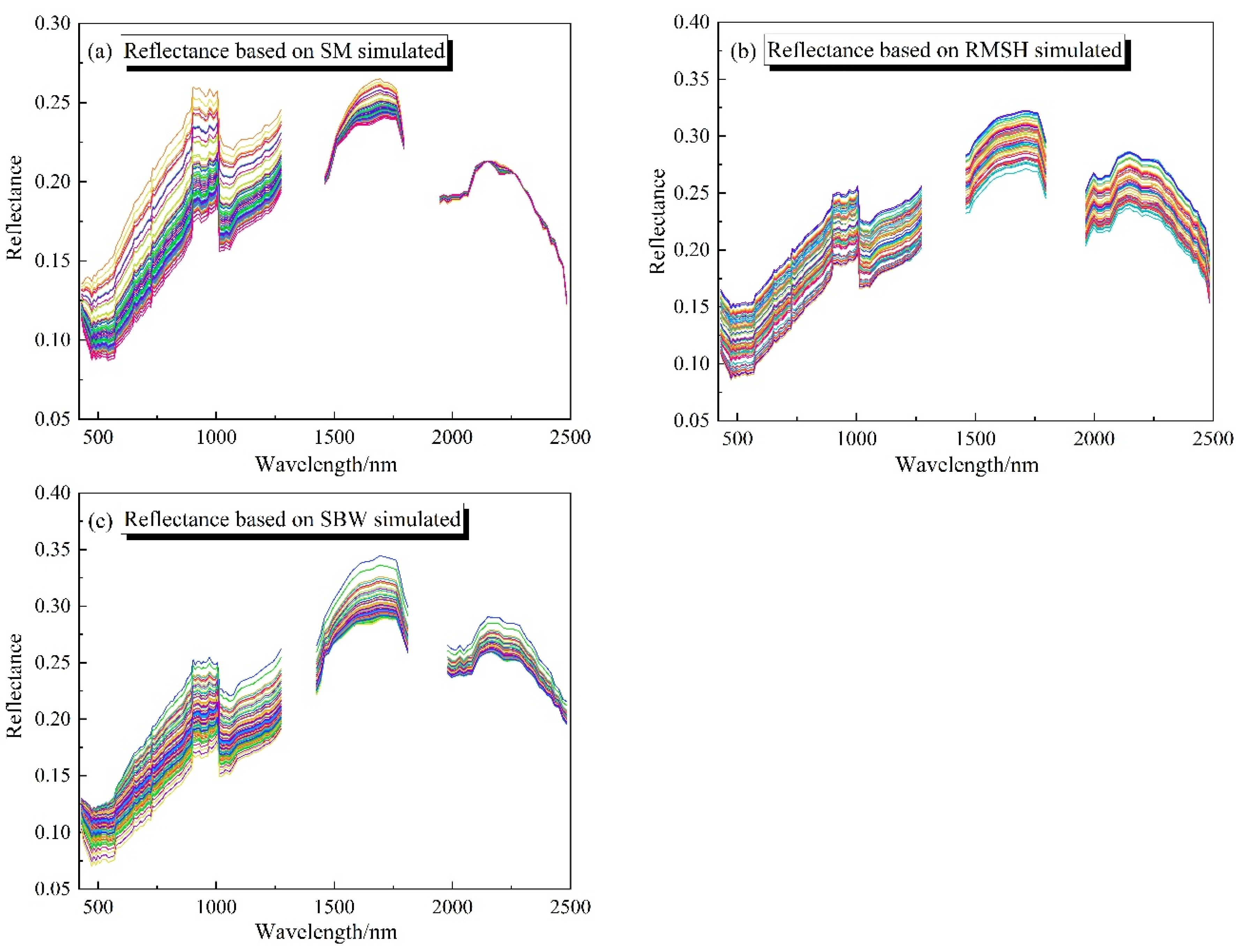
Figure 8.
The validation set-derived accuracy of soil spectral correction based on multi-order polynomial coefficient regression.
Figure 8.
The validation set-derived accuracy of soil spectral correction based on multi-order polynomial coefficient regression.
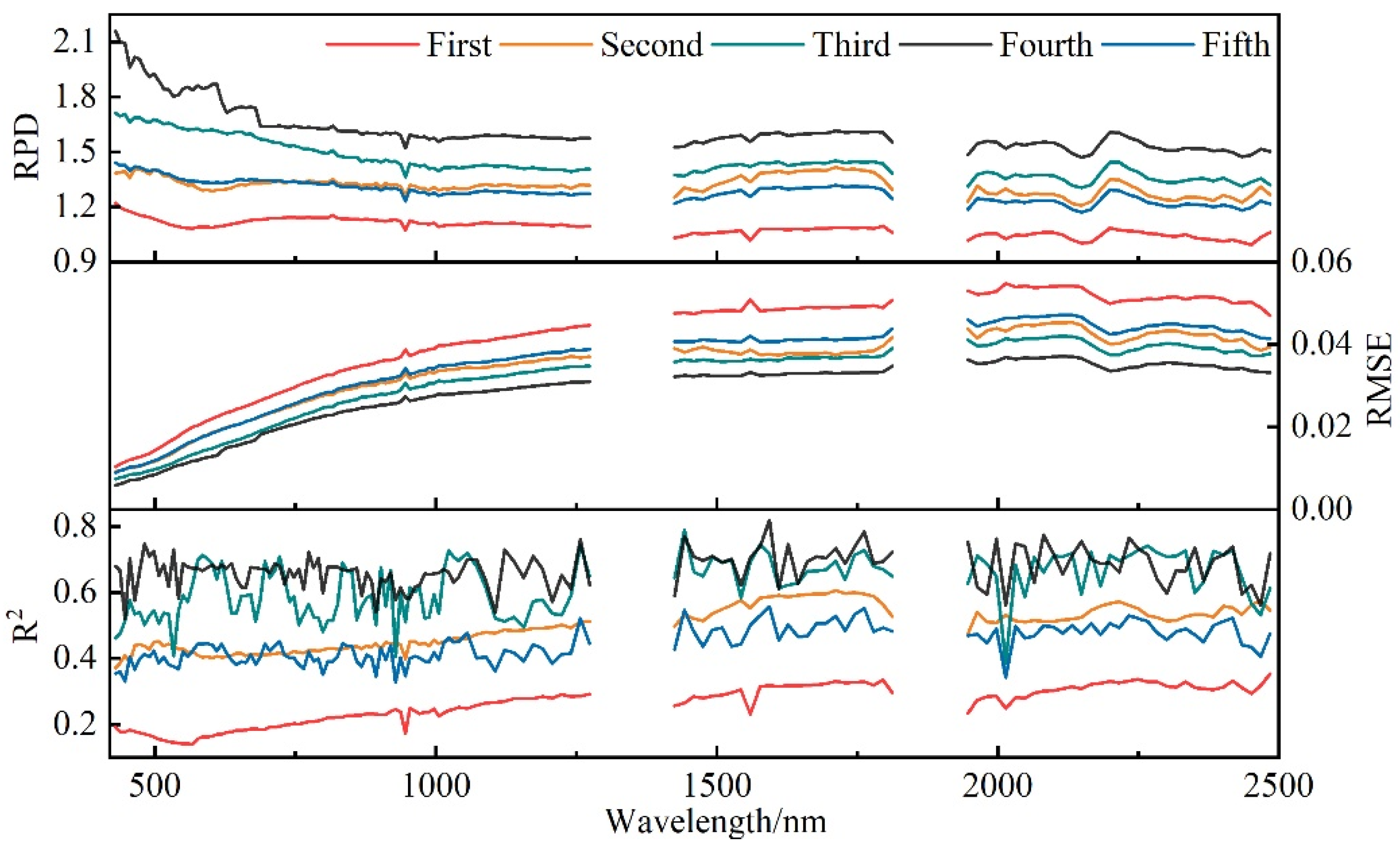
Figure 9.
The validation set-derived accuracy of soil spectral correction based on machine learning models.
Figure 9.
The validation set-derived accuracy of soil spectral correction based on machine learning models.
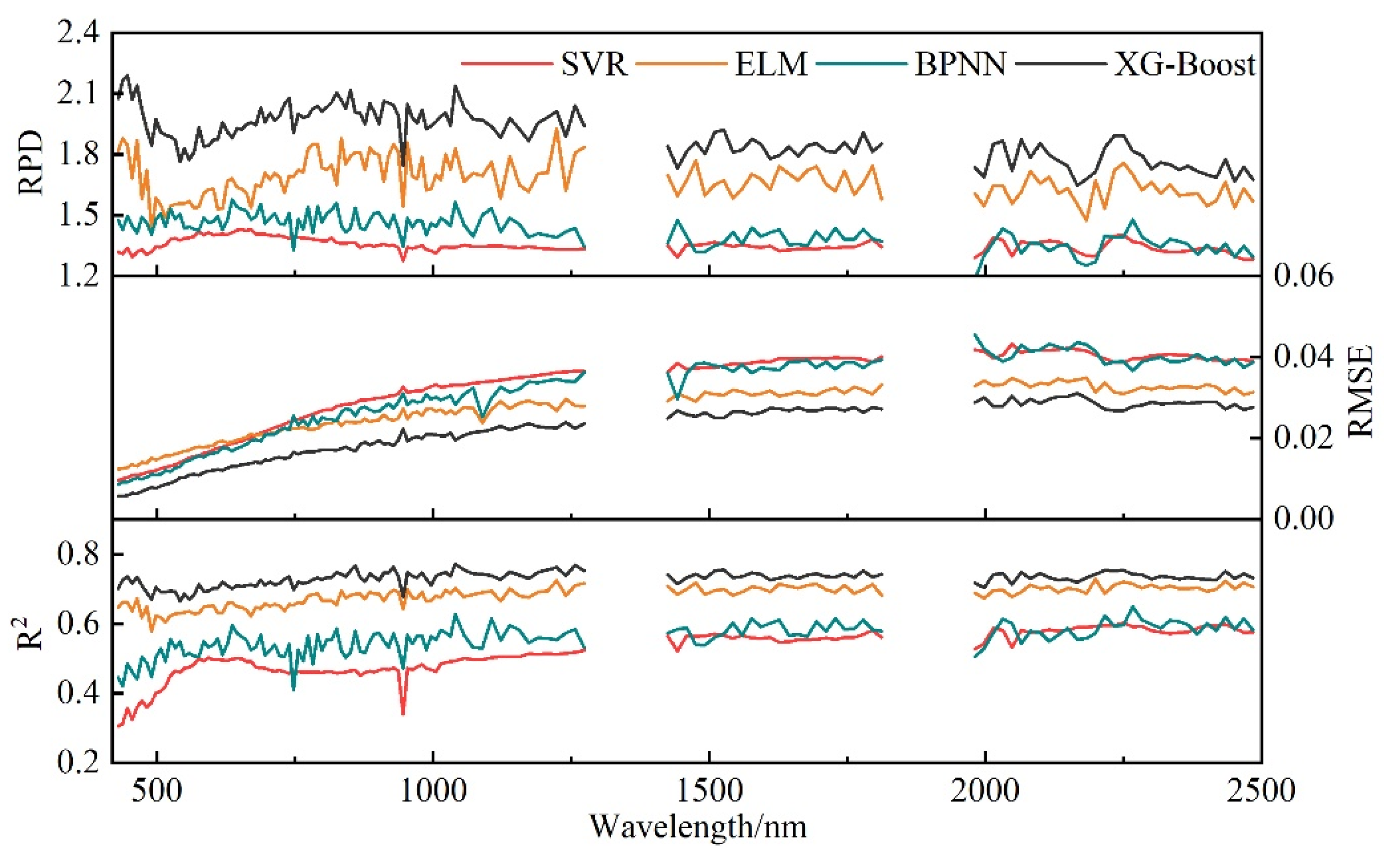
Figure 10.
Soil pixel spectra corrected with the XG-Boost model and the fourth-order polynomial model and correlation coefficients of the two sets of spectral reflectance.
Figure 10.
Soil pixel spectra corrected with the XG-Boost model and the fourth-order polynomial model and correlation coefficients of the two sets of spectral reflectance.
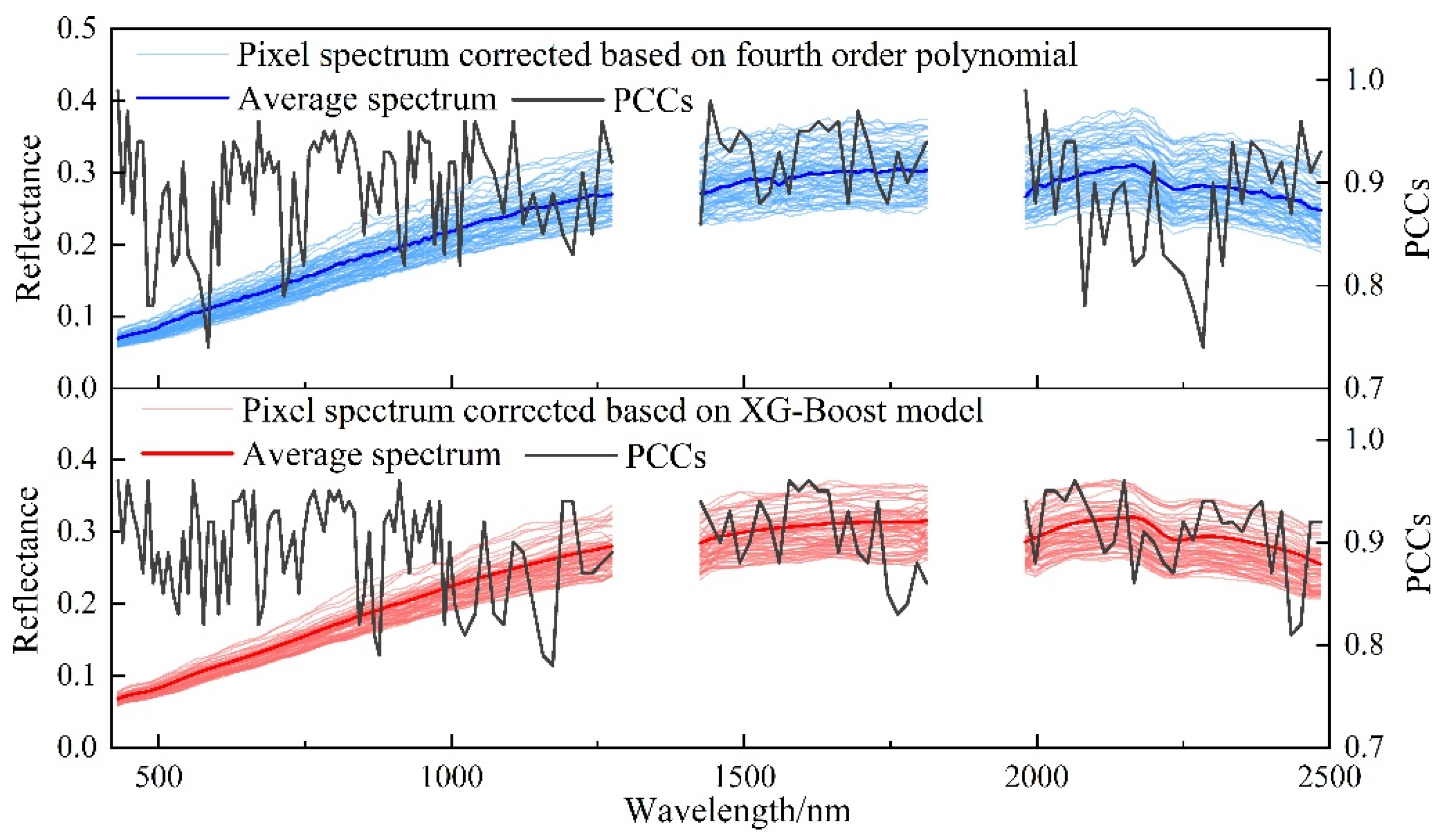
Figure 11.
(a) Pearson’s correlation coefficients between SOM contents and spectral reflectance of each band. (b) RMSECV (unit: g/kg) of multiple regression with different CARS iterations.
Figure 11.
(a) Pearson’s correlation coefficients between SOM contents and spectral reflectance of each band. (b) RMSECV (unit: g/kg) of multiple regression with different CARS iterations.
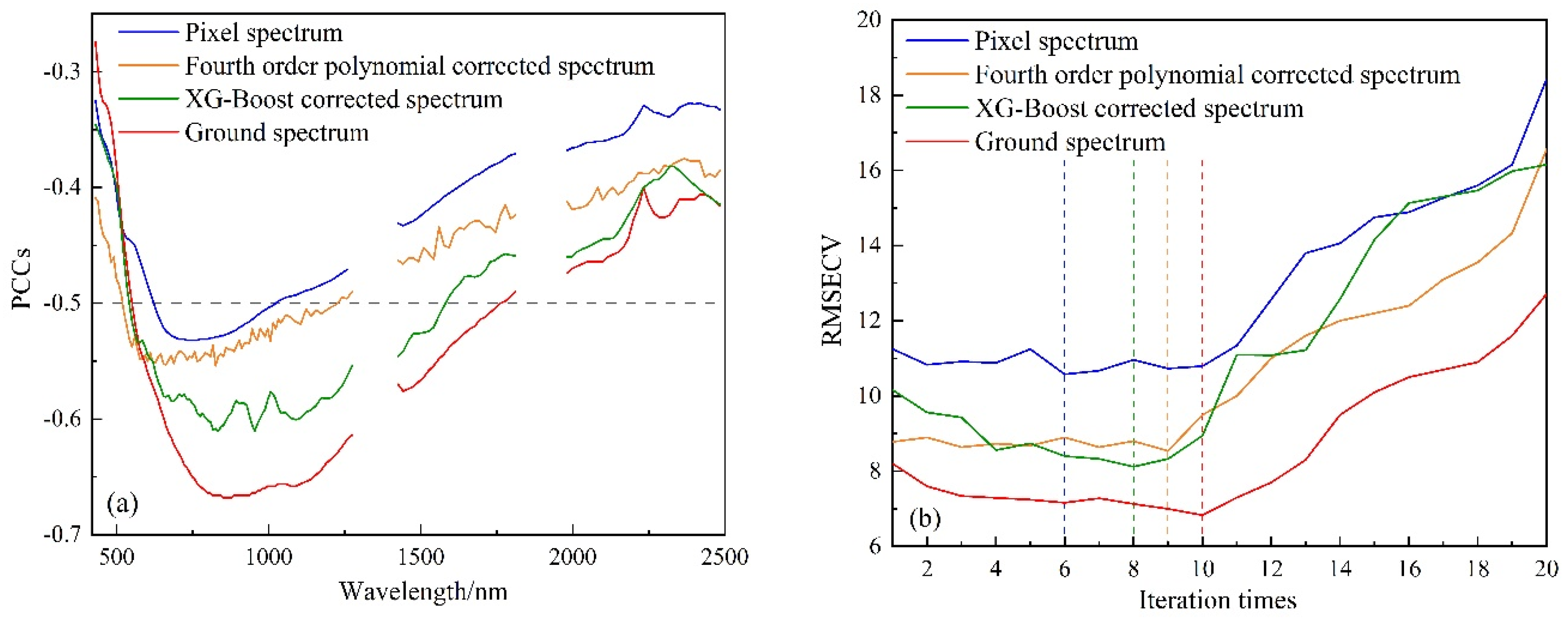
Figure 12.
Scatter plots of predicted and measured SOM contents based on the four spectral data.
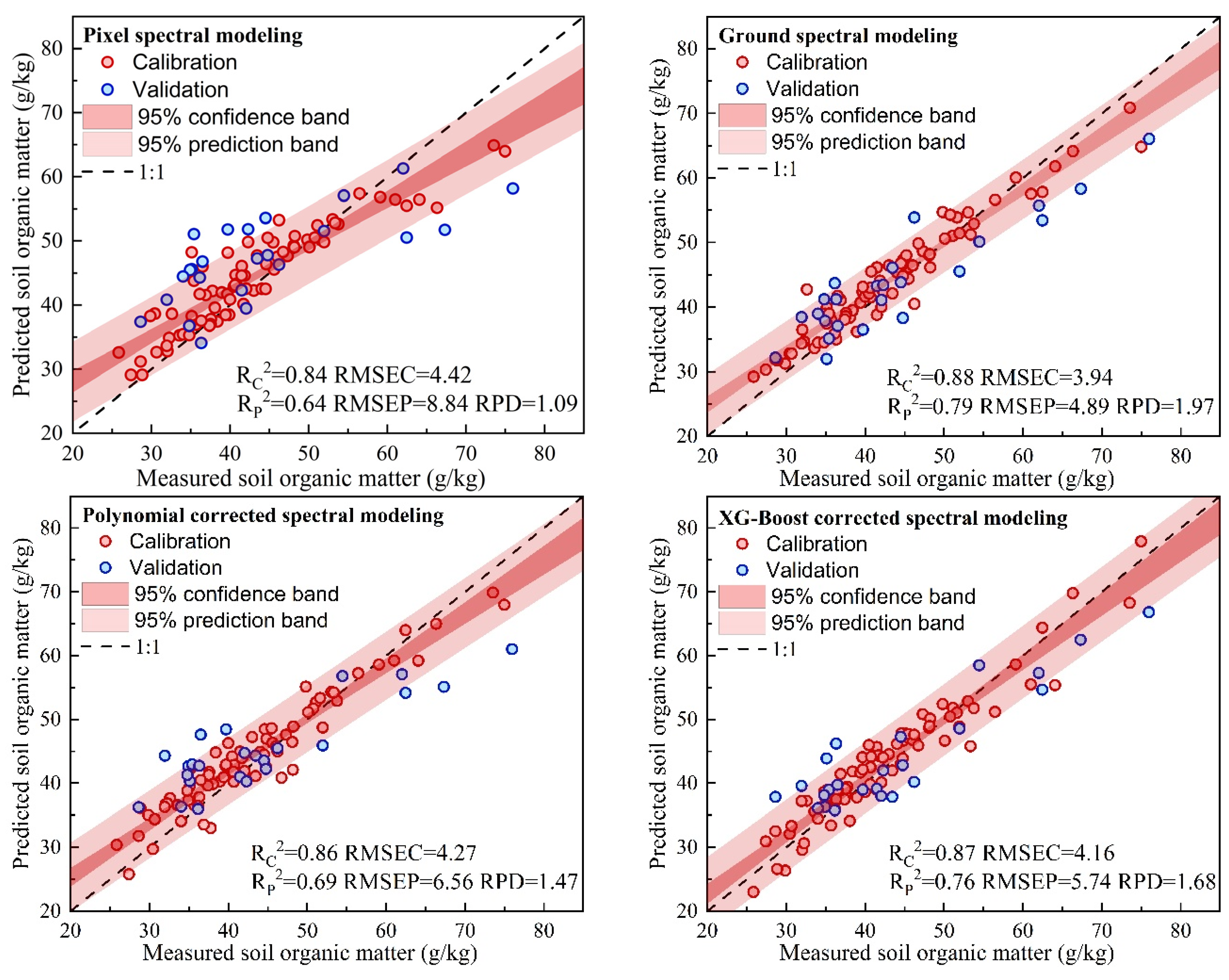
Figure 13.
Soil pixel spectra corrected with the XG-Boost model and fourth-order polynomial model, and the RPD of two correction models.
Figure 13.
Soil pixel spectra corrected with the XG-Boost model and fourth-order polynomial model, and the RPD of two correction models.
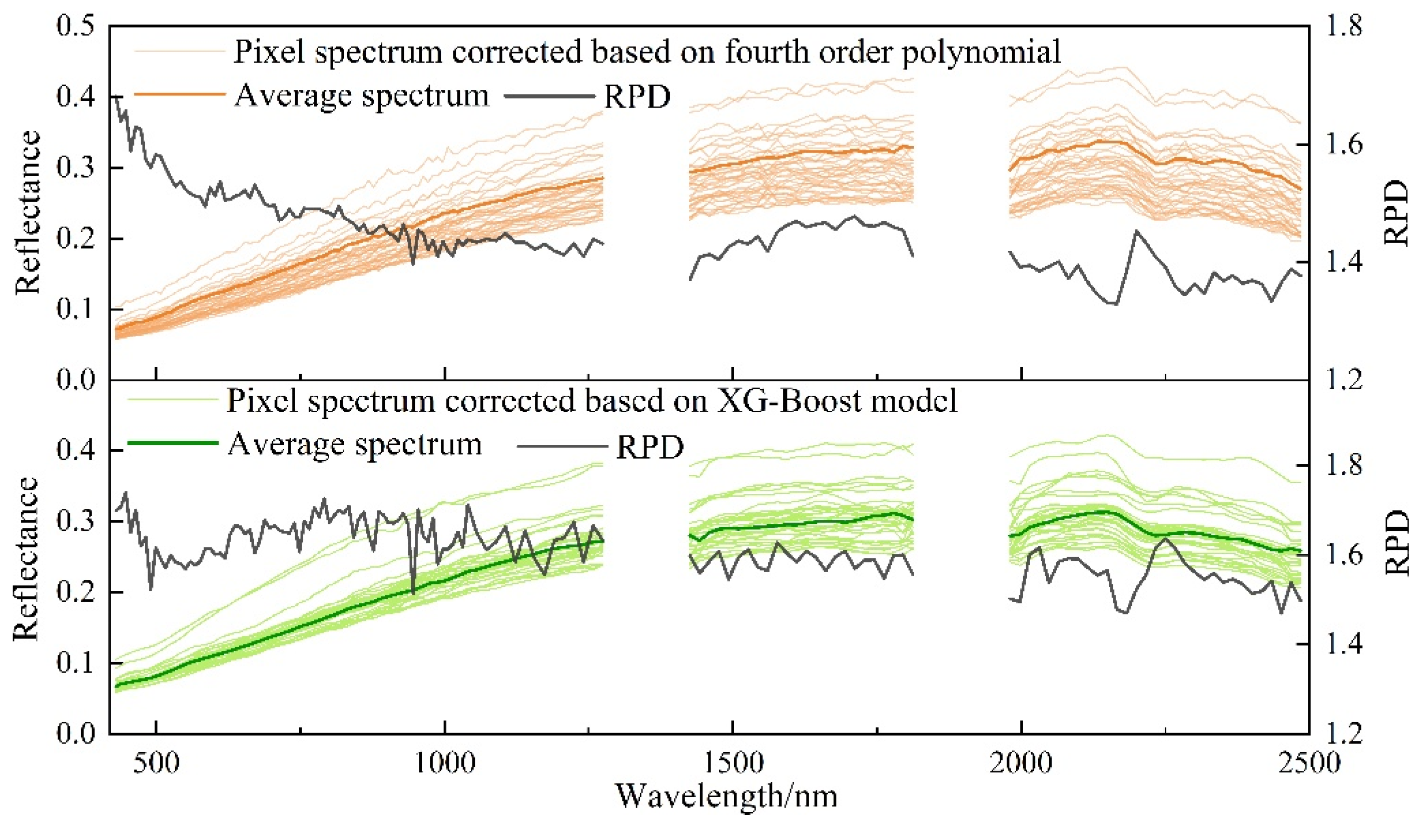
Figure 14.
Scatter plots of the measured and predicted SOM contents based on (a) original pixel spectrum, (b) ground spectrum, (c) fourth-order polynomial corrected spectrum, and (d) XG-Boost corrected spectrum with Site 2 data, using the XG-Boost model established using Site 1 data.
Figure 14.
Scatter plots of the measured and predicted SOM contents based on (a) original pixel spectrum, (b) ground spectrum, (c) fourth-order polynomial corrected spectrum, and (d) XG-Boost corrected spectrum with Site 2 data, using the XG-Boost model established using Site 1 data.
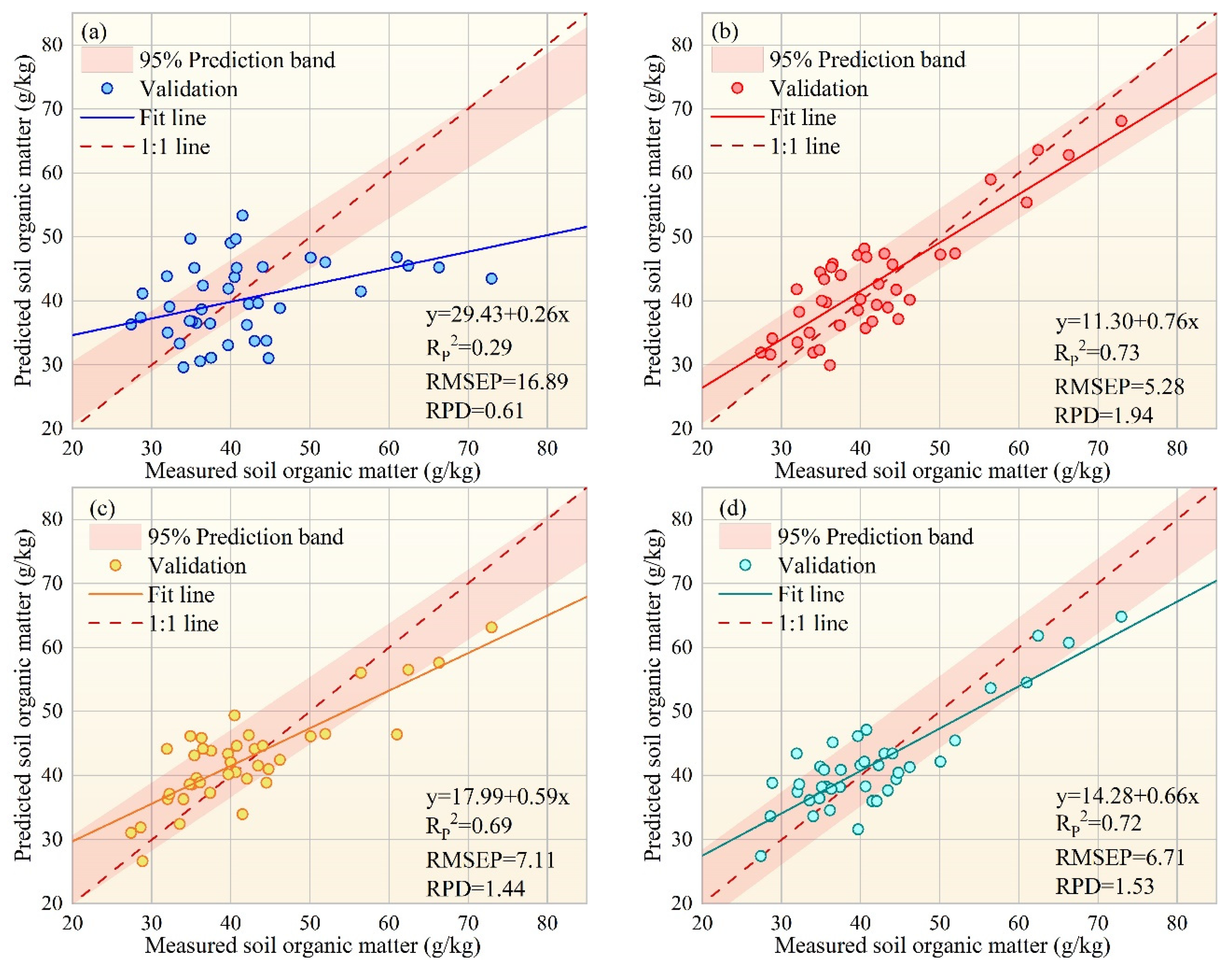
Figure 15.
Contribution rate of soil properties (SM, RMSH, and SBW) to the estimated SOM bias in Site 1 (a) and Site 2 (b). “Random” denotes the part that these three variables cannot explain.
Figure 15.
Contribution rate of soil properties (SM, RMSH, and SBW) to the estimated SOM bias in Site 1 (a) and Site 2 (b). “Random” denotes the part that these three variables cannot explain.
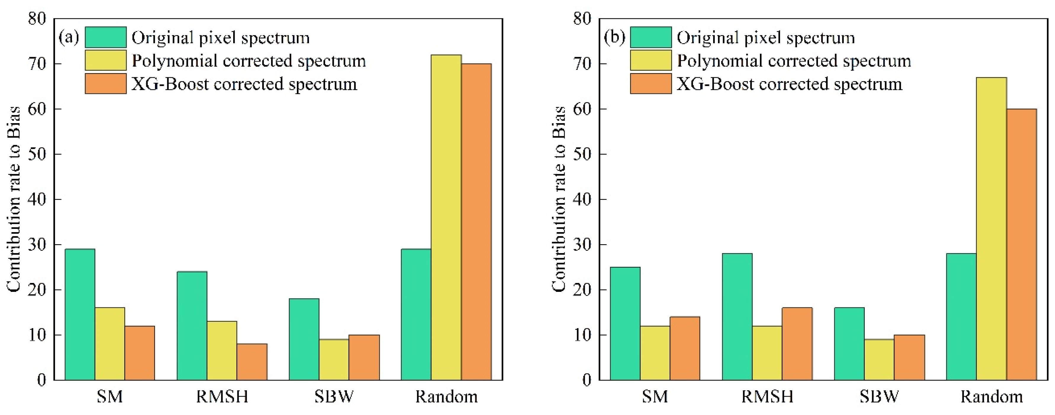

Table 1.
ZY1-02D satellite hyperspectral camera parameters.
| Specification | Parameters |
|---|---|
| Spectral range (nm) | 400-2500 |
| Channels | 76 (VNIR), 90 (SWIR) |
| Spectral resolution (nm) | 10 (VNIR), 20 (SWIR) |
| Swath width (km) | 60 |
| Spatial resolution (m) | 30 |
| Revisit cycle (d) | 3 |
| Lateral swing capacity (°) | ±26 |
Table 2.
Statistics of soil physical parameters and SOM content at the two sites.
| Dataset | Unit | Site 1 | Site 2 | ||||||||
|---|---|---|---|---|---|---|---|---|---|---|---|
| Min | Max | Mean | SD | CV % | Min | Max | Mean | SD | CV % | ||
| SM | cm3/cm3 | 0.14 | 0.47 | 0.25 | 0.08 | 31.99 | 0.21 | 0.63 | 0.37 | 0.14 | 37.93 |
| RMSH | cm | 1.32 | 4.99 | 2.49 | 0.77 | 30.92 | 2.04 | 5.78 | 3.65 | 1.34 | 36.71 |
| SBW | g/cm3 | 0.71 | 1.41 | 0.98 | 0.15 | 15.31 | 0.85 | 1.51 | 1.13 | 0.18 | 15.92 |
| SOM | g/kg | 25.84 | 75.97 | 43.25 | 10.51 | 24.30 | 27.40 | 72.97 | 41.57 | 10.28 | 24.72 |
Table 3.
Feature band statistics based on CARS.
| Spectral correction method | Wavelength (unit: um) | Total |
|---|---|---|
| Pixel spectrum | 0.67, 0.68, 0.70, 0.72, 0.74, 0.77, 0.79, 0.84, 0.87, 0.90, 0.93 | 11 |
| Fourth-order polynomial corrected spectrum | 0.55, 0.60, 0.62, 0.68, 0.73, 0.76, 0.78, 0.82, 0.85, 0.87, 0.91, 0.96, 0.99, 1.07 | 14 |
| XG-Boost corrected spectrum | 0.55, 0.62, 0.64, 0.69, 0.73, 0.77, 0.81, 0.83, 0.87, 0.89, 0.92, 0.94, 0.99, 1.05, 1.17 | 15 |
| Ground-based spectrum | 060, 0.63, 0.67, 0.70, 0.73, 0.77, 0.81, 0.85, 0.87, 0.90, 0.91, 0.96, 0.99, 1.03, 1.08, 1.22 | 16 |
Disclaimer/Publisher’s Note: The statements, opinions and data contained in all publications are solely those of the individual author(s) and contributor(s) and not of MDPI and/or the editor(s). MDPI and/or the editor(s) disclaim responsibility for any injury to people or property resulting from any ideas, methods, instructions or products referred to in the content. |
© 2024 by the authors. Licensee MDPI, Basel, Switzerland. This article is an open access article distributed under the terms and conditions of the Creative Commons Attribution (CC BY) license (https://creativecommons.org/licenses/by/4.0/).
Copyright: This open access article is published under a Creative Commons CC BY 4.0 license, which permit the free download, distribution, and reuse, provided that the author and preprint are cited in any reuse.


