Submitted:
12 February 2025
Posted:
13 February 2025
You are already at the latest version
Abstract
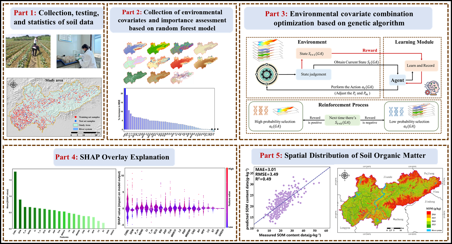
Studying the spatial variation patterns and influencing factors of soil organic matter (SOM) in hilly and basin areas is of great significance for guiding agricultural production practices. This study takes Lanxi City as an example and comprehensively considers soil formation factors such as climate, vegetation, and terrain. Based on the genetic algorithm, 47 environmental variables are combined and optimized to construct a random forest (RF) model and an improved version—a random forest model based on genetic algorithm variable combination optimization (RF-GA). At the same time, the SHAP interpretation method is used to quantitatively analyze the spatial distribution characteristics of the SOM content and further identify the main driving factors. Compared with the ordinary Kriging (OK) and random forest (RF) methods, the random forest model (RF-GA) based on genetic algorithm variable combination optimization demonstrates a significantly improved prediction accuracy (R² = 0.49; RMSE = 3.49 g·kg⁻¹), with an MAE = 3.019 and LCCC = 0.67. Among the three models, the R² of the RF-GA model increases by 87.84% and 56.29%. The model prediction results indicate that the SOM content in the study area ranges from 12.11 to 31.38 g · kg ⁻¹, showing spatial distribution characteristics of a higher content in mountainous areas and a lower content in plains. A further SHAP analysis shows that terrain, climate, and biological factors are key environmental factors affecting the spatial differentiation of the SOM, with the CNBL and DEM playing particularly significant roles. By regulating moisture, erosion deposition, vegetation distribution, and microclimate conditions, they significantly affect the spatial distribution of the SOM. In summary, the RF-GA and its interpretable prediction model constructed in this study not only effectively reveal the spatial and driving mechanisms of SOM in hilly and basin areas but also provide a solid theoretical basis and practical guidance for accurate mapping, the formulation of sustainable utilization strategies for soil resources, and ensuring national food security.
Keywords:
soil organic matter
; genetic algorithm
; random forest
; SHAP
1. Introduction
Soil organic matter (SOM) is an active and critical component of the soil carbon pool, and its spatial distribution characteristics are of great significance for revealing regional soil quality and global carbon cycling processes [1]. However, due to the combined effects of structural and stochastic factors, the spatial distribution of SOM exhibits significant variability and non-stationarity, causing significant uncertainty in modeling and quantitatively describing its spatial variation process [2]. Therefore, although it is necessary to accurately obtain spatial distribution information on regional SOM, many challenges remain in practical operation.
The soil properties in hilly basin areas often exhibit complex spatial variability and non-stationarity, making it particularly difficult to quantitatively describe soil morphology, properties, process variability, and spatial correlations [3]. Therefore, digital soil mapping (DSM) has been widely used in recent years as an important technology for quickly and accurately determining the spatial distribution of regional soil attributes [4]. However, due to the combined influence of natural soil-forming factors and human activities, the SOM in farmland often exhibits significant spatial non-stationarity, which further increases the difficulty of SOM spatial prediction [5]. Identifying the key influencing factors of the SOM spatial distribution and introducing them into prediction models can greatly improve prediction accuracy.
Traditional soil attribute mapping methods, such as Kriging interpolation, inverse distance weight interpolation, spline function interpolation, and other geostatistical methods [6], as well as the commonly used Kriging and regression analysis methods, often use linear estimation methods, which have difficulty in capturing the complex nonlinear relationship between SOM and environmental variables [7]. Therefore, in recent years, an increasing number of scholars have begun to introduce machine learning algorithms, such as support vector machines (SVMs), random forests (RFs), artificial neural networks (ANNs), and regression trees, aiming to more accurately establish the nonlinear relationship between SOM and environmental variables [8,9]. These methods typically rely on sample data and environmental covariates for fitting, with the commonly used environmental variables including soil type, climate factors, land use type, vegetation index, terrain factors, and soil parent material [10,11]. Terrain factors in particular have a significant impact on SOM content by regulating surface runoff, solar radiation, soil erosion, moisture content, and temperature, making them particularly important in hilly and mountainous areas [12].
The genetic algorithm (GA) is a global optimization algorithm that simulates the natural evolution process, continuously optimizing variable combinations through operations such as selection, crossover, and mutation in order to select feature sets that can maximize model performance [13]. In complex terrain and multivariate environments, the GA can effectively avoid becoming stuck in local optima, thereby improving the robustness and accuracy of model predictions [14]. However, the random forest model based on GA filtering features (GA-RF) has not been fully applied in SOM estimation in complex areas, and its advantages in SOM prediction over the RF model using full-variable prediction still need to be verified. Therefore, this study proposes a random forest model based on the genetic algorithm for variable combination optimization, aiming to improve the prediction accuracy of the SOM spatial distribution in complex regions and provide new perspectives and methods for DSM research.
Although machine learning methods typically outperform traditional statistical methods in terms of prediction accuracy, their “black box” nature—i.e., their lack of sufficient interpretability—has always limited their practical applications. To address this issue, the SHAP (Shapley Additive exPlans) method based on game theory and local interpretation theory was introduced to quantitatively estimate the contribution of each feature variable to the model’s prediction results [15]. In the field of soil property simulation, SHAP has not only successfully identified key driving factors but has also effectively analyzed the interactions between different climate and terrain variables, making it widely used to interpret the prediction results of complex models [16].
Lanxi City is located in the central and western part of Zhejiang Province, and it is the largest Yangmei producing area in the region, with a typical hilly and basin landform. Identifying the main controlling factors of the SOM in farmland in Lanxi City and obtaining a high-precision SOM spatial distribution map will help not only to formulate scientific and reasonable farmland planting and management strategies, optimize land use layouts, increase soil carbon sequestration capacities, and alleviate the greenhouse effect but also to enhance soil fertility and achieve increased grain production.
The main objectives of this study are to (1) explore the potential application of GA-RF models based on variable combination optimization in DSM in complex regions; (2) evaluate the performance differences between this model and the ordinary Kriging method (OK) and the RF model based on full-variable prediction in terms of predicting the SOM spatial distribution; and (3) use the SHAP method to analyze the spatial correlation between SOM formation environmental variables and SOM content.
2. Research Area and Data Sources
2.1. Overview of the Study Area
Lanxi City is located in the central and western part of Zhejiang Province, with the geographical coordinates of 29°1′20″–29°27′30″ north latitude and 119°13′30″–119°53′50″ east longitude; it has a total area of 1313 square kilometers. The climate belongs to the subtropical monsoon region of East Asia, with abundant annual precipitation. The landform is a hilly basin in central Zhejiang, surrounded by mountains in the northeast, winding low hills in the southwest, and a flat plain in the central part. The main soil types in the research area are red soil, yellow soil, lithological soil, tidal soil, and paddy soil, with agriculture being the main land use.
2.2. Data Sources and Processing
2.2.1. Soil Sample Data
Surface soil samples were collected in 2022. Before conducting field investigations, soil sample points were evenly distributed in the study area based on field surveys, effectively reflecting the distribution characteristics of the agricultural land soil properties in the study area. The soil sample points were set up in advance using the grid sampling method. Firstly, to meet the soil sample size requirement, a 2 × 2 km regular grid was generated in the exploration area, and points were generated at the center of each grid to obtain uniformly distributed grid points. Next, to remove the grid points in the non-agricultural land area, actual measurement data were used to extract agricultural map layers for the preliminary screening of the grid points. Considering the complex agricultural landscape in the research area, the selected grid points were overlaid with high-resolution images from Google Earth to visually determine the land use type and further screen the grid points. A total of 1566 surface soil and crop samples were ultimately collected. For soil sampling, the upward drilling method was adopted, and a 10 m × 10 m grid was established at each sampling point, with a sampling depth of 0–20 cm. Ten soil cores were randomly selected at each point using a 5 cm diameter spiral soil drill, and all soil cores were mixed into one soil sample.
After the field investigation was completed, the soil samples collected via air drying and crushing were filtered through a 1.0 mm sieve and stored in sealed glass jars for further analysis. Finally, the SOM content was measured using the potassium dichromate volumetric method. To reduce the interference of a few outliers in the data analysis, the organic matter data of 1566 samples from Lanxi City were checked and removed as outliers in Excel software. Finally, 1560 sampling points were determined, and their spatial distribution is shown in Figure 1. In ArcGIS 10.2, 80% of the samples were randomly and uniformly selected as the training set (1249), and the remaining 20% were selected as the validation set (311).
2.2.2. Obtaining Environmental Covariates
Based on the soil landscape SCORPAN function model [17], following the principles of correlation and availability, soil texture, terrain factors, remote sensing biological indices, climate factors, soil types, and land use were selected as environmental variables to predict the soil properties in the study area, as shown in Table 1. According to McBratney et al. [18], of the digital mapping studies, 80% have used terrain elements, 25% have used biological elements, another 25% have used parent rock elements, 5% have used climate elements, and none have used time elements.
- (1)
- Topographical factors
The terrain series of soil is mainly controlled by surface morphology characteristics and parent rocks, which are relatively uniform in a small area. Therefore, terrain is the most important influencing factor in the formation of local soil. Terrain factors directly affect the energy cycle of surface materials and the occurrence and evolution of soil, and they are commonly used environmental variables in soil mapping. This study used 12.5 m digital elevation model (DEM) data for terrain data, and, based on these DEM data, the slope, aspect, profile curvature, plane curvature, terrain roughness index (TRI), total catchment area (TCA), stream power index (SPI), topographic wetness index (TWI), multiscale ridge top flatness (MRRTF), multiscale valley bottom flatness (MRVBF), etc., were extracted using SAGA-GIS 7.6.2 software. Among them, MRRTF and MRVBF are humidity indices that identify flat and low terrain or high flat areas at multiple resolutions by progressively smoothing and coarsening the DEM while reducing slope thresholds to identify valleys or ridges. These terrain factors affect the movement of surface materials and energy from different aspects, thereby influencing the soil formation process.
- (2)
- Climate factors
The annual average temperature, the annual average precipitation, and other climate factors were sourced from the National Qinghai Tibet Plateau Data Center in China http://data.tpdc.ac.cn (14 May 2022). The dataset was generated by downscaling in China based on the gridded time series climate dataset released by the Climate Research Unit (CRU) at the University of East Anglia in the UK, as well as the WorldClim global high-resolution climate dataset [19].
- (3)
- Biological factors
Biological factors indirectly reflect the surface conditions and vegetation landscape characteristics formed by soil properties through the characteristic bands and different combinations of remote sensing images. Remote sensing image data were obtained from Sentinel-2, which involves high-resolution multispectral imaging satellites carrying a multispectral imager (MSI) for land monitoring. Sentinel-2 can provide images of vegetation, soil and water cover, inland waterways, and coastal areas and involves two satellites: 2A and 2B. This study used Sentinel-2A satellite data, with a spatial resolution of 10m, downloaded from the GEE (Google Earth Engine) public data platform. The image time was consistent with the sampling time, and the cloud cover was 0. Subsequently, the obtained image data underwent preprocessing such as format conversion, projection transformation, and resampling. Information on the frequency bands of Sentinel-2 is shown in Table 2.
- (4)
- soil texture
Soil texture is one of the physical properties of soil, referring to the combination of mineral particles of different sizes and diameters in the soil. Soil texture is closely related to soil aeration, fertilizer retention, the water retention status, and the difficulty of cultivation, and its condition is an important basis for formulating soil utilization, management, and improvement measures. Fertile soil requires not only a good texture of the plow layer but also a good texture profile. Although soil texture is mainly determined by the type of parent material and is relatively stable, the texture of the cultivated layer can still be adjusted through activities such as tillage and fertilization. The spatial distribution data of soil texture were compiled based on soil type maps and soil profile data obtained from soil surveys, and they were divided into three categories, namely, sand, silt, and clay, each of which reflects the content of particles with different textures through percentages. The dataset was provided by the Geographic Remote Sensing Ecological Network Platform (www.gisrs.cn), and it has a spatial resolution of 900m.
- (5)
- Soil type and land use data
The soil type and land use data were sourced from the measured data collected in this experiment. This study used arithmetic mean transformation for categorical variables, such as land use and soil type, which allowed for the quantitative relationship between the levels of the independent variables and the quantitative outcome variables to be established using the relationship between the categorical independent variables and quantitative dependent variables. The arithmetic mean (area percentage) of the quantitative dependent variable under different land use and soil types was used to replace the land use and soil types.
3. Research Method
3.1. Ordinary Kriging
Ordinary Kriging (OK) is an accurate spatial local interpolation method based on the theory of variation functions [20,21]. In OK, a theoretical semi-variogram model of the regionalized variable is first fitted with the observed values. The value at the predicted point can be obtained by linearly weighting the observed values within a certain range around it, while the weight value is determined under the guidance of unbiased and optimal thinking. The calculation formula for OK is as follows:
Here, is the OK estimate at , is the observation at , and is the weight value. The OK method determines the optimal weight value on the premise of unbiasedness (the estimated value equal to the true value) and optimality (minimum variance), thus satisfying the following conditions:
Unbiased condition:
Optimal condition:
3.2. Random Forest
Random forest (RF) is a tree structure model that adopts an ensemble learning strategy, which can be used for both the classification and prediction of continuous variables [22]. In recent years, the random forest (RF) algorithm, as an excellent machine learning algorithm, has been widely used in digital soil mapping research based on multi-source environmental variables. RF-based models are non-parametric models and can handle the complex nonlinear relationship between soil properties and environmental covariates [23]. Moreover, RF has low sensitivity to the noise present in training samples; thus, it can better handle the problem of reduced accuracy caused by data loss and identify the importance of predictive variables [24]. Numerous studies have shown that RF has a higher prediction accuracy than other machine learning algorithms and traditional statistical regression methods [25].
Its advantages are that it does not require the assumption that the dependent variable is normally distributed, and it does not require testing for multicollinearity between independent variables. More importantly, it can explore the nonlinear relationship between independent and dependent variables. The RF model uses the bootstrap method to perform random sampling with replacement from the original training set, forming m new training sets and independently constructing CART decision tree models using each new training set. The samples remaining each time are called out-of-bag data. n independent variables are randomly selected from each tree to determine the classification of tree nodes. The final prediction result is determined by voting on the prediction results of all trees (when the dependent variable is a categorical variable) or by taking the average (when the dependent variable is a continuous variable). RF calculates the increase in the mean square error (MSE) of the regression equation to predict the out-of-bag data when removing each variable, % IncMSE, and it determines the relative importance of each variable based on this: the higher the % IncMSE, the more important the variable [26]. The RF model has two key parameters: the number of trees (ntree) and the number of nodes (mtry). When the computational load allows, a larger ntree is better; changes in mtry will affect the goodness of fit of the model, and multiple attempts will be required (ranging from 1 to the number of independent variables).
3.3. Genetic Algorithm
The genetic algorithm (GA) is a random search optimization algorithm based on natural selection and genetic mechanisms, inspired by the theory of biological evolution. It simulates genetic operations (selection, crossover, mutation, etc.) to achieve the iterative process from the initial population to the optimal solution [27]. In variable combination optimization problems, the GA encodes variable combinations into chromosomes (such as binary encoding, where each gene corresponds to a variable) to achieve feature selection or optimization [28]. The algorithm starts from a randomly generated initial population; evaluates the quality of each chromosome through fitness functions, such as prediction accuracy and AIC/BIC indicators; and then uses selection, crossover, and mutation operations to generate new populations during the iteration process, continuously optimizing the quality of the solution. The optimization objectives of the GA typically include maximizing model performance (such as accuracy or minimum error), minimizing the number of variables to simplify the model, and ensuring the robustness of the results. This process outputs the optimal variable combination after meeting the predetermined termination conditions, such as the number of iterations or the convergence of fitness [29]. The GA has a wide range of applications in feature selection and variable combination optimization due to its powerful global search capability and adaptability to complex high-dimensional nonlinear problems. The principle of GA algorithm is shown in Figure 2.
3.4. SHAP Driving Force Analysis
SHAP is a game theory-based method proposed by Lundberg and Lee to describe the performance of machine learning models, it uses Shapley values to estimate the contribution value of each feature [30]. According to game theory, each feature variable in a dataset can be seen as the result of a member training a model using that dataset to obtain predictions, and it can be seen as the benefit of all members working together to complete a project. The Shapley value provides a fair distribution of the benefits of cooperation by considering the contributions of each member. Due to the use of Shapley values from game theory as explanatory measures, an SHAP attribution analysis has the advantages of strong global and local interpretability of variables, a fair distribution of variable contributions, and excellent visualization effects, which compensate for the poor interpretability of black box models. Therefore, SHAP is introduced to explain and analyze the nonlinear relationship between a single variable and the dependent variable through the Shapley value and to evaluate the contributions of various environmental variables.
Let us assume the use of groups (with features) to predict the output of the RF model. In SHAP, the contribution of each feature to the model output is allocated based on its marginal contribution. The Shapley value is determined by using the following formula:
In the formula, is the Shapley value of feature ; is the set of all features; is the set of all feature subsets produced from after removing feature ; refers to the probability weight of derived after feature permutation and combination; and and represent sets of the feature subsets. The features and predicted values of model are input, and its prediction is compared with that of the current input , where represents the values of the input features in set .
3.5. Model Evaluation Indicators
Four indicators were selected to evaluate the predictive performance of the model: the mean absolute error (MAE), the root mean square error (RMSE), the coefficient of determination (R2) of the linear regression equation between the predicted and observed values, and Lin’s consistency correlation coefficient (LCCC). Their calculation formulas are as follows:
Among them, is the number of sample points in the validation set, is the observed value at sample point i, is the predicted value at sample point i, is the average of the observed values, is the average of the predicted values, r is the Pearson correlation coefficient between the observed and predicted values, is the standard deviation of the observed values, and is the standard deviation of the predicted values. Among them, the and measure the numerical error of the prediction set, with smaller values indicating a higher model prediction accuracy. Moreover, mainly reflects whether the predicted trend is correct; the larger the value, the more accurate the model’s predicted trend. On the basis of measuring correlations (Pearson correlation coefficient), also considers prediction bias; that is, it comprehensively considers the prediction accuracy and trend of the model [31,32].
Therefore, its results are more reliable. The range of LCCC values is between 0 and ± 1. The larger the value, the closer the predicted and observed point pairs are to the perfect consistency line (45° diagonal) in the scatter plot. When the absolute value of LCCC is equal to 1, it indicates perfect consistency (or perfect inconsistency); when LCCC is equal to 0, it indicates no correlation. Overall, a good predictive model has lower MAE and RMSE values and higher R2 and LCCC values.
4. Experimental Results and Analysis
4.1. Basic Statistics of Soil Organic Matter Content
The distribution characteristics and variability of data have an impact on the reliability of spatial interpolation results. In Kriging interpolation, if the data follow a normal distribution, the optimal prediction results can be obtained [33]. Therefore, normality testing and transformation of the data were performed to obtain more reliable prediction results.
This study first conducted descriptive statistics on the soil organic matter content of the training and validation sets, and it performed K-S tests on the experimental data in SPSS 26. The results (Table 2) show that the maximum value (Max), minimum value (Min), average value (AVE), and standard deviation (SD) of the training and validation sets were relatively consistent. The magnitude of the coefficient of variation (CV) indicates the spatial variability of soil properties. When the coefficient of variation is less than 10%, it suggests weak variability; when the coefficient of variation is greater than 100%, it suggests strong variability. A value between the two suggests moderate variability. According to Table 3, the soil organic matter in the study area belongs to a moderately variable type.
Based on the skewness and kurtosis values, as well as the K-S value (K-S) test results, it could be concluded that both the training and validation sets are non-normally distributed. Although Kriging interpolation does not strictly require data to be normally distributed, when the data deviate too far from the normal distribution, the interpolation effect may not be ideal. After performing Box–Cox transformation (Box–Cox) on the training and validation sets, the skewness and kurtosis values were close to 0, and the K-S test results were greater than 0.05, thus conforming to the normal distribution.
4.2. Assessment of the Importance of Environmental Variables in RF Models
The optimal parameters of a random forest are determined using the grid search method. Grid search traverses all possible combinations within a preset hyperparameter range to find the optimal hyperparameter combination [34]. This method can quickly find a relatively good hyperparameter setting, but it may require significant computational resources and time. The optimal parameters for the RF model in this study were mtry = 19 and ntree = 500, and the optimal parameters for the RFGA model were mtry = 4 and tree = 500. Based on the RF model, the importance ranking of all environmental variables involved in modeling was conducted, and it was found that there were differences in the importance of the effects of the different environmental variables on the prediction results of different attribute spaces. In the RF model importance evaluation results (% IncMSE) of the soil SOM content, the order of influence on the SOM from high to low was as follows (Figure 3): the CNBL, DEM, Tm, LSTMm, Hm, MSAVI, WEI, E-m, SCD, BSI, etc. Therefore, the two factors that had the greatest impact on the SOM in the RF results were the CNBL and DEM.
4.3. Comparative Analysis of Mapping Accuracy
After obtaining the SOM (Box–Cox transformation) spatial prediction results of each prediction model, inverse transformation can be used to obtain the SOM spatial distribution results based on Kriging interpolation. RF uses 47 full variables to predict soil organic matter across the entire domain. The optimal variable combination selected by GA-RF is P_m, E_m, VARI, NDWI, NPP, MNDWI, GNDVI, BSI, AH, ASP, CI, CNBL, CND, DEM, LS, MRRTF, RSP, TCA, LU, ST, and SCD, predicting soil SOM across the entire region based on 21 environmental variables.
The prediction results of each model are externally validated using the MAE, RMSE, R2, and LCCC, as shown in Table 4. It can be observed that, among the three types of prediction models, the OK model has higher MAE and RMSE values, while R2 and LCCC are very low, indicating that using only the Kriging method results in poor prediction accuracy and trends. In the regression model, according to the LCCC results, the order from best to worst for each model is RF-GA > RF > OK. These results indicate that the RF-GA model considering nonlinear relationships has the smallest spatial interpolation error, OK has the largest spatial interpolation error, and RF-GA and RF have improved interpolation accuracy compared to OK due to the use of auxiliary variables.
4.4. SHAP Overlay Explanation
Figure 4 shows the distribution of the SHAP values for each environmental variable, with positive values indicating a positive impact on the SOM content and negative values indicating a negative impact on the SOM content. As shown in Figure 5, the importance of SR, VARI, GNDVI, and NDVI is relatively low, and the SHAP values are concentrated around 0. However, the importance of the CNBL and DEM is relatively high, with a wide distribution range of SHAP values. The bee colony plot in Figure 5 shows that the CNBL and DEM have a significant impact on the SOM content.
According to the results of the environmental variable driving force analysis of the soil organic matter content in the study area, terrain factors, climate factors, and biological factors are important environmental variables that affect the spatial distribution of the SOM in the study area, which is consistent with the conclusion of RF. Among them, terrain factors reflect not only the regional environment but also the influence of hydrogeological features on the distribution of soil properties. Climate factors not only directly affect the decomposition rate of soil organic matter but also indirectly affect soil organic matter content by influencing soil moisture content and vegetation type. Biological factors affect the distribution of organic matter through vegetation cover and growth conditions.
4.5. Spatial Distribution of Soil Organic Matter
The prediction accuracy of the optimization model based on the combination of RF and GA variables is relatively high, achieving an R2 of 0.49, an MAE of 3.01 g·kg−1, an RMSE of 3.49 g·kg−1, and an LUCC of 0.67. The fitting with actual values indicates that the model can effectively predict the SOM content. To allow for a visual comparison of the SOM prediction results of different models, we display the prediction results of all models within the same range (Figure 6, Figure 7 and Figure 8). The SOM content in the predicted graph exhibits a significant spatial variability in distribution. The prediction results indicate that, in the study area, the SOM content is higher in the northern and eastern mountainous areas, while it is lower in the central area with a flat terrain, and a few high values are also distributed in southern cities and mixed forest areas. In the northern and eastern mountainous areas, the main land cover type is forest, with dense vegetation and a complex terrain; less human intervention allows vegetation to continuously input organic matter into the soil, and the mountainous terrain may slow down soil erosion, resulting in a higher accumulation rate of organic matter in the soil. The flat areas in the central region are mainly farmland, and more agricultural activities such as long-term cultivation and fertilization may accelerate the decomposition of organic matter. In addition, areas with a flat terrain are more susceptible to rainfall and wind erosion, further reducing the SOM content.
The prediction results of the three models are shown in Figure 4. It can be seen that the SOM spatial distribution prediction results of RF and RF-GA are very similar. The difference is that the OK prediction results are very smooth, while the RF and RF-GA prediction models can highlight the spatial details and changes in the SOM, demonstrating richer SOM spatial variation information. The OK valuation significantly differs from the original data. The areas exhibiting high SOM are mainly distributed in areas with significant terrain fluctuations, which is conducive to the accumulation of SOM.
5. Discussion
5.1. Advantages of RF-GA Model
Compared with the traditional OK and RF methods based on full-variable prediction, the RF-GA method used in this study has the following advantages: Firstly, it addresses the issue of spatial heterogeneity in complex regions, improving the ability to understand data features and achieving a better fitting accuracy, even without distinguishing land use types. In addition, this model has significant advantages over the OK and RF methods in predicting the SOM in complex areas. Compared with RF, the RF-GA model can effectively screen out environmental covariates with high contributions to the model, avoiding the interference of variables with low contributions on model accuracy and significantly improving the accuracy of SOM prediction.
5.2. Explanation of Environmental Variables
The influencing factors of SOM vary greatly among regions under the influence of natural and human disturbances [35]. Terrain, climate, and biological factors have become key influencing factors of the SOM in the hilly basin area of Lanxi City, and they exhibit a certain degree of threshold or peak effects. The CNBL and DEM have the greatest impact on the SOM, a similar conclusion to that drawn in related studies [36,37,38]. Terrain factors regulate the soil organic matter distribution by influencing the water content, erosion deposition, vegetation distribution, and the microclimate [39]. Climate factors affect the accumulation and decomposition of soil organic matter through temperature, precipitation, vegetation, and microbial activity. Warm and humid environments accelerate decomposition, while cold and arid regions promote accumulation. Biological factors affect the soil organic matter distribution through vegetation growth, litter input, and biological activity [40].
5.3. Limitations and Potential Improvements
5.3.1. Insufficient Data Scale and Representativeness
This study is based on a data analysis of 1560 sampling points in Lanxi City. The limited sample size and spatial distribution may affect the universality of the model prediction. In addition, environmental variables such as climate variables do not fully take into account temporal dynamic changes. In the future, the predictive ability of the model can be improved by increasing the number of sampling points, expanding the research area, and introducing a time series analysis.
5.3.2. Improvement Directions for Model Optimization
Although genetic algorithms effectively improve model performance, they have high computational complexity and longer variable optimization time. At the same time, both the RF and RF-GA models exhibit sparse samples of extreme values. This is because, in the spatial distribution of soil properties, extreme values often correspond to special geographical conditions or environmental factors, and these areas may have fewer sampling points. Random forests cannot fully capture the complex features of these sparse areas, resulting in a tendency to approach the mean of the global data when predicting, thereby narrowing the range of the predicted values. By optimizing the model and data in the future, combined with subsequent correction methods, this phenomenon can be alleviated.
5.3.3. Lack of Applicability and Interaction Analysis of Explanatory Methods
The SHAP interpretation method effectively analyzes the contribution of environmental variables to SOM, but it has high computational complexity and resource consumption. Furthermore, this study did not delve into the interactions between environmental factors. In the future, a lightweight explanatory model can be considered, combined with SHAP interaction values, to further analyze the coupling relationship of environmental variables.
6. Conclusions and Prospects
This study was based on a soil investigation and measured data, with Kriging interpolation (OK), a random forest (RF) model, a random forest model based on genetic algorithm variable combination optimization (RF-GA), and the SHAP interpretation method (SHAP) used to analyze the spatial differentiation characteristics and key influencing factors of the SOM in Lanxi City, as well as the impact of their effects. The following important conclusions were obtained:
- (1)
- The distribution of the SOM in the research area is influenced by factors such as terrain, climate, and biological factors, and it has obvious spatial differentiation characteristics. In the study area, the SOM content is higher in the northern and eastern mountainous areas, while it is lower in the central area with a flat terrain. A few high values are also distributed in southern cities and mixed forest areas.
- (2)
- The random forest model RF-GA based on genetic algorithm variable combination optimization is more effective in extracting environmental variables, it demonstrates improved accuracy in SOM prediction compared to the RF model using full-variable prediction, making it a promising tool for SOM prediction in complex areas.
- (3)
- Further research using the RFGA-SHAP model indicates that the key influencing factors on the spatial distribution of surface SOM in the hilly basin area of Lanxi City are CNBL, DEM, Pm, NDWI, CI, Tm, SCD, BSI, etc. These factors can make significant contributions to soil management practices and provide information for decision-making to promote sustainable land use and agricultural productivity.
Author Contributions
Conceptualization, H.H. and Z.T; Methodology, H.H. and Y.X.; Software, Z.T; Validation, Y.L. and Z.R.; Formal analysis, Z.T.; Investigation, H.H; Resources, Z.R. and Y.L. Data curation, Z.R. and Y.L.; Writing-original draft, H.H.; Writing-review & editing, Y.X. and Z.T.; Visualization, Y.X. and Y.L.; Supervision, Y.L; Funding acquisition, Y.L. All authors haveread and agreed to the published version of the manuscript.
Funding
The authors acknowledge the support of the project “the Key Program of National Natural Science Foundation of China” (42230107);“National Natural Science Foundation of China”(42471454); and ”Strategic Science and Technology Talent Cultivation Special Project of Hubei province”(2024DJA012).
Data Availability Statement
The original contributions presented in the study are included in thearticle, further inquiries can be directed to the corresponding author.
Conflicts of Interest
The authors declare no conflicts of interest.
References
- Wiesmeier, M.; Barthold, F.; Blank, B.; et al. Digital mapping of soil organic matter stocks using Random Forest modeling in a semi-arid steppe ecosystem[J]. Plant & Soil 2011, 340, 7–24. [Google Scholar] [CrossRef]
- Kempen, B.; Brus, D.J.; Stoorvogel, J.J.; et al. Efficiency Comparison of Conventional and Digital Soil Mapping for Updating Soil Maps[J]. Soil Science Society of America Journal 2012, (revisions)(6). [Google Scholar] [CrossRef]
- Zhao, M.S.; Rossiter, D.G.; Li, D.C.; et al. Mapping soil organic matter in low-relief areas based on land surface diurnal temperature difference and a vegetation index[J]. Ecological Indicators 2014. [Google Scholar] [CrossRef]
- Zhao, M.S.; Rossiter, D.G.; Li, D.C.; et al. Mapping soil organic matter in low-relief areas based on land surface diurnal temperature difference and a vegetation index[J]. Ecological Indicators 2014. [Google Scholar] [CrossRef]
- Xie, H.; Li, W.; Duan, L.; et al. Digital mapping of cultivated land soil organic matter in hill-mountain and plain regions[J]. Journal of soil & sediments 2024, 24. [Google Scholar] [CrossRef]
- Zhang, W.C.; Wan, H.S.; Zhou, M.H.; et al. Soil total and organic carbon mapping and uncertainty analysis using machine learning techniques[J]. Ecological Indicators 2022, 143. [Google Scholar] [CrossRef]
- Sun, Y.; Ma, J.; Zhao, W.; et al. Digital mapping of soil organic carbon density in China using an ensemble model[J]. Environmental research, 231(Pt 2):116131[2025-02-06]. [CrossRef]
- Mousavi, S.R.; Sarmadian, F.; Omid, M.; et al. Three-dimensional mapping of soil organic carbon using soil and environmental covariates in an arid and semi-arid region of Iran[J]. Measurement 2022. [Google Scholar] [CrossRef]
- Zeraatpisheh, M.; Ayoubi, S.; Jafari, A.; et al. Digital mapping of soil properties using multiple machine learning in a semi-arid region, central Iran[J]. Elsevier 2019. [Google Scholar] [CrossRef]
- Agyeman, P.C.; Ahado, S.K.; Boruvka, L.; et al. Trend analysis of global usage of digital soil mapping models in the prediction of potentially toxic elements in soil/ sediments: a bibliometric review[J]. Environmental Geochemistry and Health 2021, 42. [Google Scholar] [CrossRef]
- Hendriks C M J, Stoorvogel J J, lvarez-Martínez, Jose Manuel, et al. Introducing a mechanistic model in digital soil mapping to predict soil organic matter stocks in the Cantabrian region (Spain)[J]. European Journal of Soil Science 2021, 72. [Google Scholar] [CrossRef]
- Sun, X.L.; Wang, H.L.; Zhao, Y.G.; et al. Digital soil mapping based on wavelet decomposed components of environmental covariates[J]. Geoderma 2017, 303, 118–132. [Google Scholar] [CrossRef]
- Min, H.; Ko, H.J.; Ko, C.S. A genetic algorithm approach to developing the multi-echelon reverse logistics network for product returns[J]. Omega 2006, 34, 56–69. [Google Scholar] [CrossRef]
- Maziar, Pasdarpour, and,et al. Optimal design of soil dynamic compaction using genetic algorithm and fuzzy system[J]. Soil Dynamics and Earthquake Engineering 2009. [CrossRef]
- Shapchenkova, O.A.; Krasnoshchekov, Y.N.; Loskutov, S.R. Application of the methods of thermal analysis for the assessment of organic matter in postpyrogenic soils[J]. Eurasian Soil Science 2011, 44, 677–685. [Google Scholar] [CrossRef]
- Agyeman, P.C.; Ahado, S.K.; Boruvka, L.; et al. Trend analysis of global usage of digital soil mapping models in the prediction of potentially toxic elements in soil/ sediments: a bibliometric review[J]. Environmental Geochemistry and Health 2021, 42. [Google Scholar] [CrossRef] [PubMed]
- Minasny, B.; McBratney, A.B.; Malone, B.P.; et al. Digital mapping of soil carbon[J]. Advances in agronomy 2013, 118, 1–47. [Google Scholar]
- McBratney, A.B.; Santos ML,, M.; Minasny, B. On digital soil mapping[J]. Geoderma 2003, 117, 3–52.
- Peng, S.; Ding, Y.; Liu, W.; et al. 1 km monthly temperature and precipitation dataset for China from 1901 to 2017[J]. Earth System Science Data 2019, 11, 1931–1946. [Google Scholar] [CrossRef]
- MATHERONG Estimating and Choosing [M]. Springer Berlin Heidelberg, 1989.
- WEBSTERR Geostatistics for Environmental Scientists [M]. John Wiley & Sons, 2001.
- BREIMANL Random forests [J]. Machine Learning 2001, 45, 5–32. [CrossRef]
- FORKUOR G, HOUNKPATIN O K L, WELP G, et al. High Resolution Mapping of Soil Properties Using Remote Sensing Variables in South-Western Burkina Faso: A Comparison of Machine Learning and Multiple Linear Regression Models [J]. Plos One 2017, 12. [Google Scholar]
- Were, K.; Bui, D.T.; Dick, O.B.; et al. A comparative assessment of support vector regression, artificial neural networks, and random forests for predicting and mapping soil organic carbon stocks across an Afromontane landscape [J]. Ecological Indicators 2015, 52, 394–403. [Google Scholar] [CrossRef]
- PITTMANR; HUB; WEBSTERK Improvement of soil property mapping in the Great Clay Belt of northern Ontario using multi-source remotely sensed data [J]. Geoderma 2021, 381.
- KENNEDY, WERE, DIEU, et al. A comparative assessment of support vector regression, artificial neural networks, and random forests for predicting and mapping soil organic carbon stocks across an Afromontane landscape [J]. Ecological Indicators 2015, 52, 394–403. [Google Scholar] [CrossRef]
- Salah, B.; Ali, F.; Ali, O.; et al. Optimal Deep Learning LSTM Model for Electric Load Forecasting using Feature Selection and Genetic Algorithm: Comparison with Machine Learning Approaches[J]. Energies 2018, 11, 1636. [Google Scholar] [CrossRef]
- Xue,Bing,Zhang, et al. A Comprehensive Comparison on Evolutionary Feature Selection Approaches to Classification.[J]. International Journal of Computational Intelligence & Applications 2015. [CrossRef]
- Huang, J.; Cai, Y.; Xu, X. A hybrid genetic algorithm for feature selection wrapper based on mutual information[J]. Pattern Recognition Letters 2007, 28, 1825–1844. [Google Scholar] [CrossRef]
- Lundberg, S.; Lee, S.I. A Unified Approach to Interpreting Model Predictions[J]. 2017. [CrossRef]
- Lini, K. A concordance correlation coefficient to evaluate reproducibility [J]. Biometrics 1989, 45, 255–68. [Google Scholar] [CrossRef]
- Mcbrideg, B. A proposal for strength-of-agreement criteria for Lin's concordance correlation coefficient [J]. 2005.
- Ying-Qiang, S.; Lian-An, Y.; Bo, L.; et al. Spatial Prediction of Soil Organic Matter Using a Hybrid Geostatistical Model of an Extreme Learning Machine and Ordinary Kriging[J]. Sustainability 2017, 9, 754. [Google Scholar] [CrossRef]
- Li-Na, G.; Gui-Sheng, F. Support Vector Machines for Surface Soil Density Prediction based on Grid Search and Cross Validation[J]. Chinese Journal of Soil Science 2018. [Google Scholar]
- Chen, S.; Arrouays, D.; Mulder, V.L.; et al. Digital mapping of GlobalSoilMap soil properties at a broad scale: A review[J]. Geoderma 2022, 409, 115567. [Google Scholar] [CrossRef]
- Hamzehpour, N.; Shafizadeh-Moghadam, H.; Valavi, R. Exploring the driving forces and digital mapping of soil organic carbon using remote sensing and soil texture[J]. Catena 2019, 182, 104141. [Google Scholar] [CrossRef]
- Zhao, C.; Li, P.; Yan, Z.; et al. Effects of landscape pattern on water quality at multi-spatial scales in Wuding River Basin, China[J]. Environmental Science and Pollution Research 2024, 31, 19699–19714. [Google Scholar] [CrossRef] [PubMed]
- Zhou, Y.; Zhao, X.; Guo, X.; et al. Mapping of soil organic carbon using machine learning models: Combination of optical and radar remote sensing data[J]. Soil Science Society of America Journal 2022, 86, 293–310. [Google Scholar] [CrossRef]
- Zeraatpisheh, M.; Ayoubi, S.; Jafari, A.; et al. Digital mapping of soil properties using multiple machine learning in a semi-arid region, central Iran[J]. Geoderma 2019, 338, 445–452. [Google Scholar] [CrossRef]
- Guo, P.T.; Li, M.F.; Luo, W.; et al. Digital mapping of soil organic matter for rubber plantation at regional scale: An application of random forest plus residuals kriging approach[J]. Geoderma 2015, 237, 49–59. [Google Scholar] [CrossRef]
- Keskin, H.; Grunwald, S.; Harris, W.G. Digital mapping of soil carbon fractions with machine learning[J]. Geoderma 2019, 339, 40–58. [Google Scholar] [CrossRef]
Figure 1.
Location of the research area and distribution of sampling points.
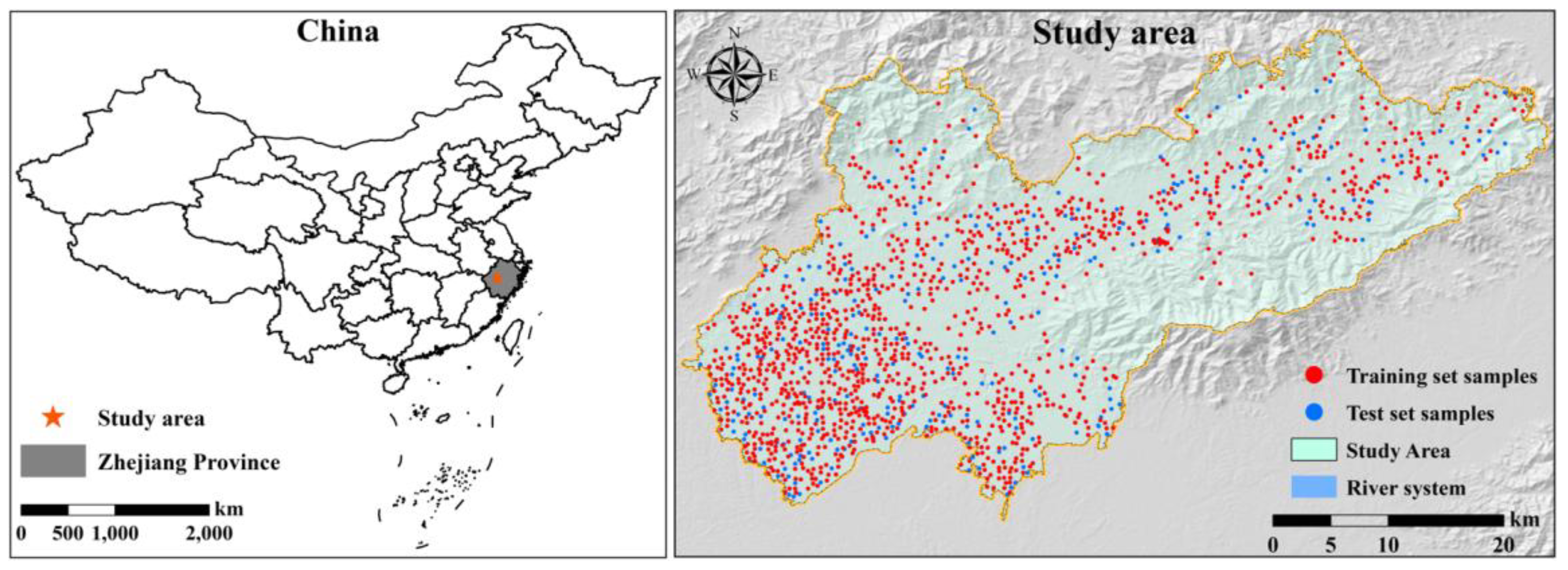
Figure 2.
Schematic diagram of the GA model structure.
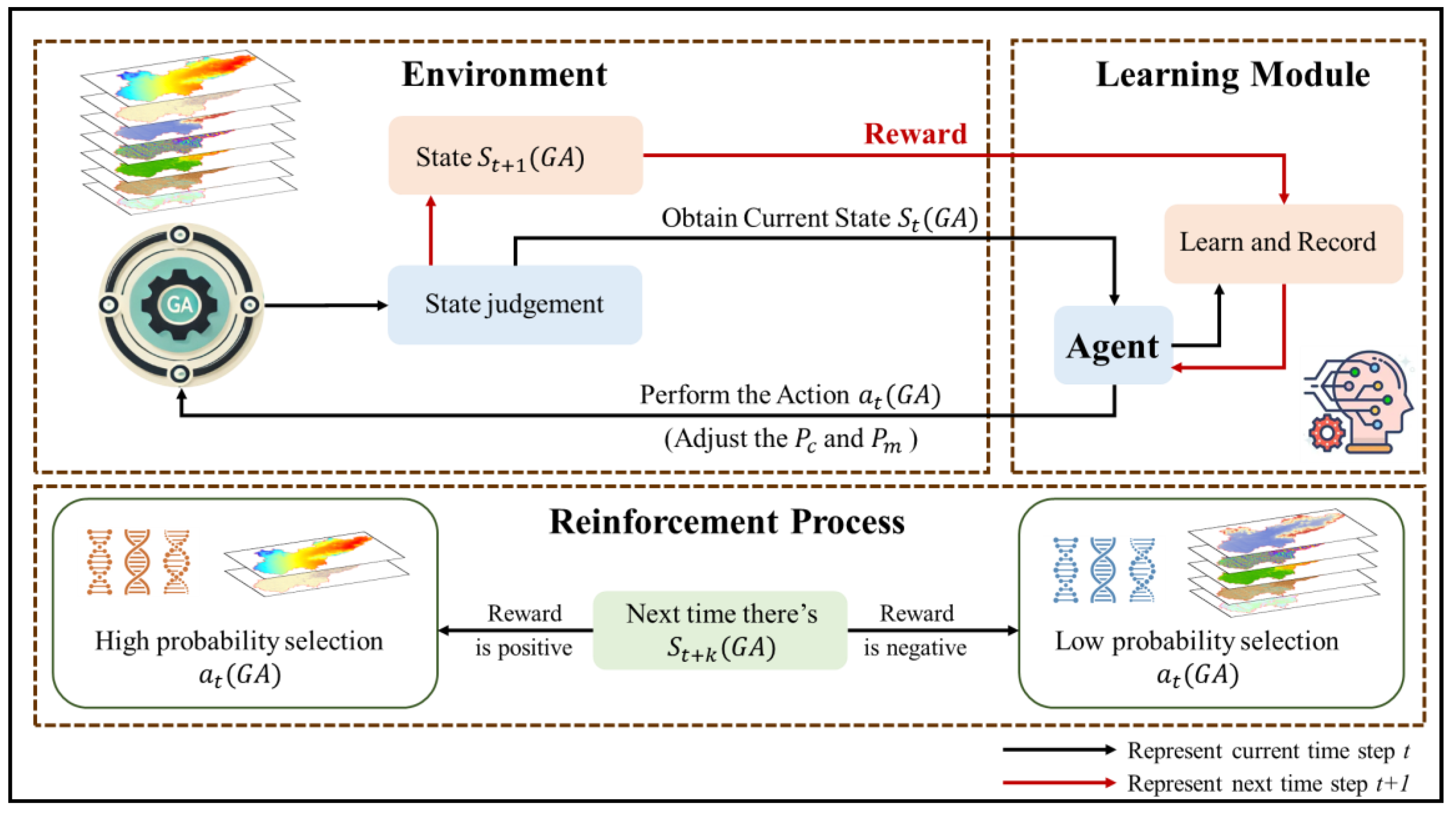
Figure 3.
Ranking of % IncMSE values of various influencing factors in the random forest model.
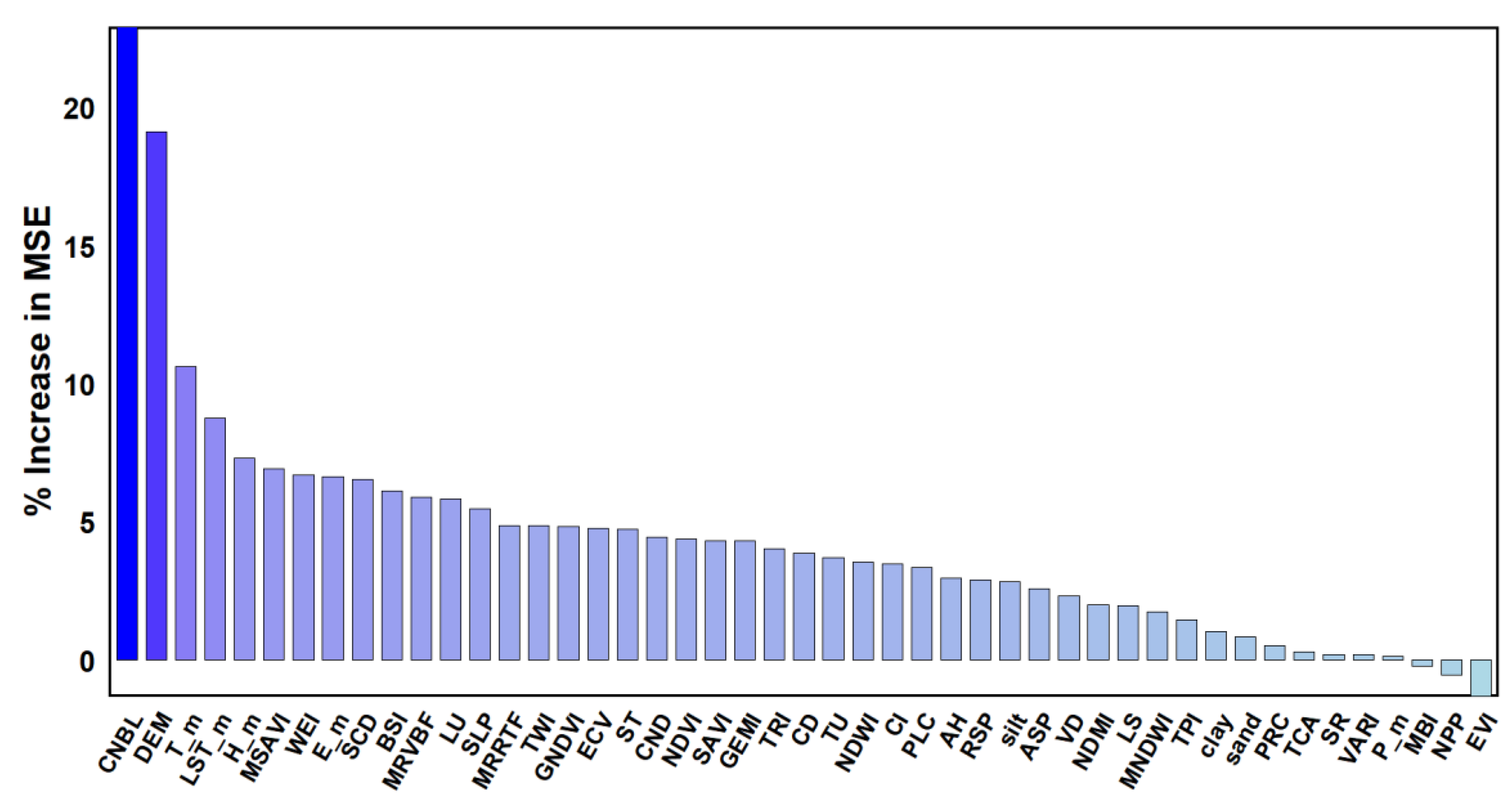
Figure 4.
Shapley values between soil organic matter content and environmental variables. The overall importance of each variable is shown, with the x-axis representing the ranking of environmental variable importance and the y-axis representing the average SHAP value of each influencing factor.
Figure 4.
Shapley values between soil organic matter content and environmental variables. The overall importance of each variable is shown, with the x-axis representing the ranking of environmental variable importance and the y-axis representing the average SHAP value of each influencing factor.
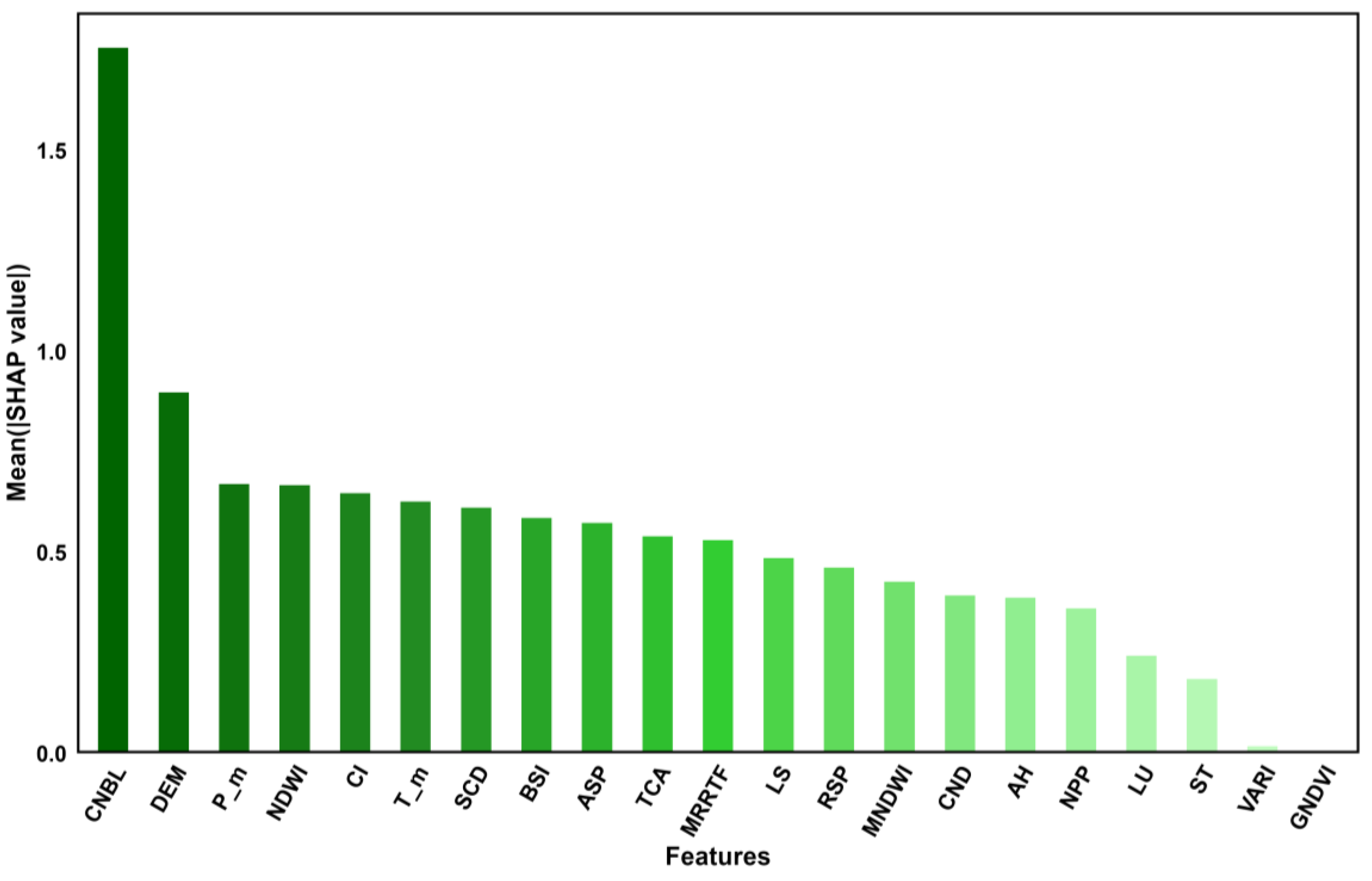
Figure 5.
Colony plot of Shapley values between soil organic matter content and environmental variables. The overall importance and direction of influence of variables are shown. Feature ranking (x-axis) represents the importance of the environmental variables, the SHAP value (y-axis) represents the unified index of the influence of a certain factor in the model, and red (blue) dots represent the value of environmental variables. SHAP > 0 represents a positive contribution. As the SHAP value increases, the positive effect of the factor on the SOM content is higher. SHAP < 0 represents a negative contribution, and, as the SHAP value decreases, the negative effect of the factor on SOM content is higher.
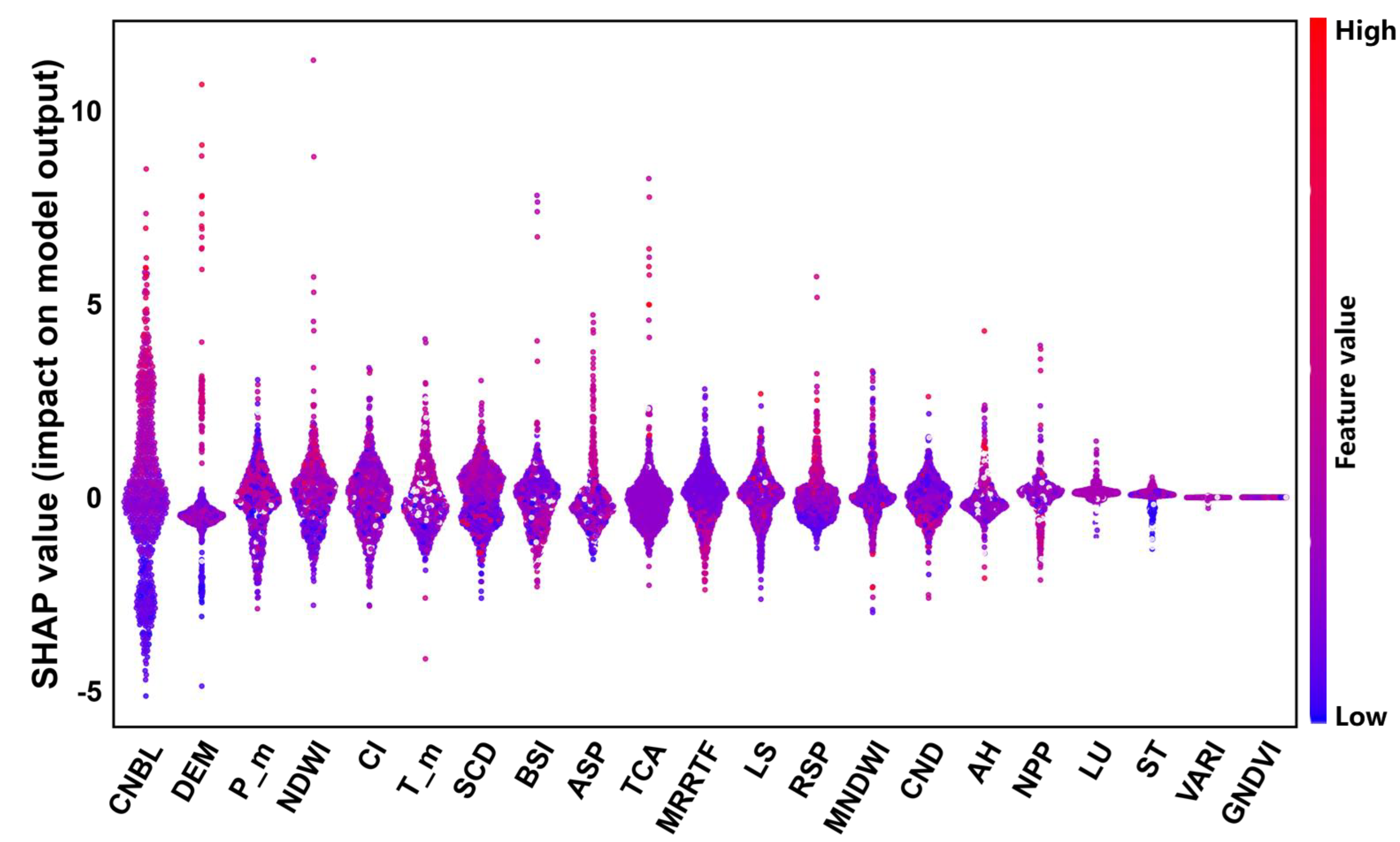
Figure 6.
Spatial distribution map of prediction accuracy of the OK model for SOM.
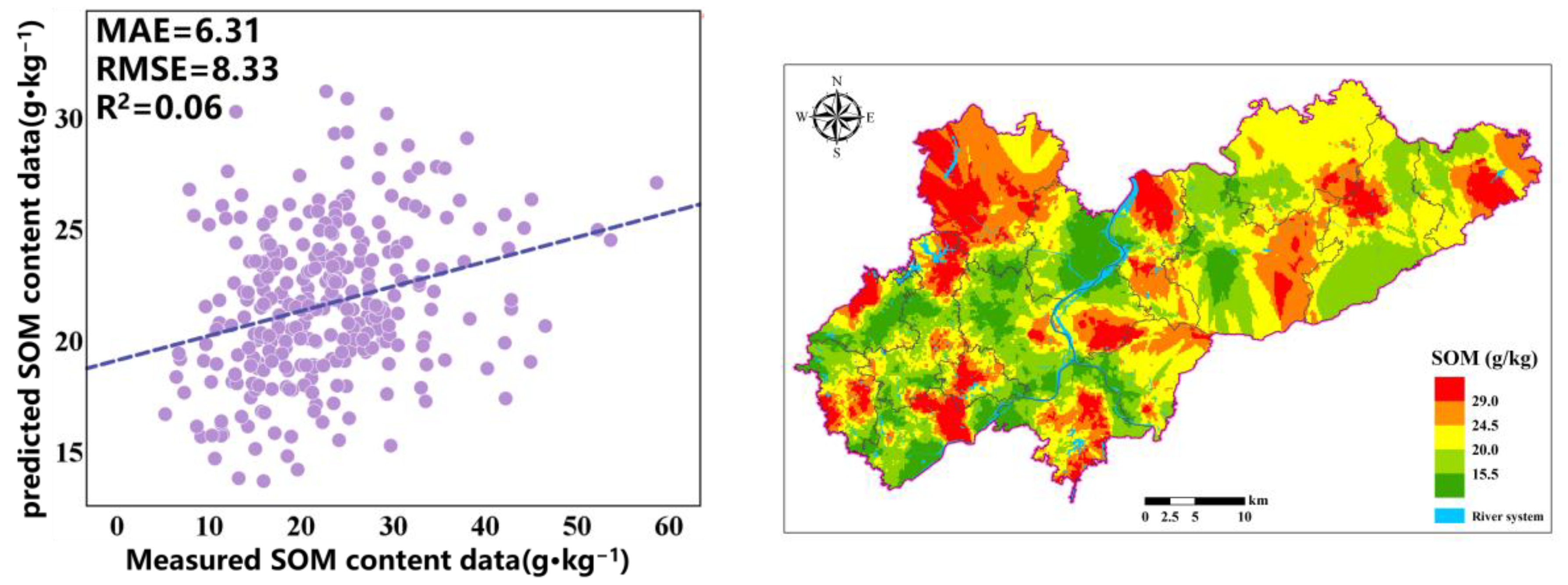
Figure 7.
Spatial distribution map of prediction accuracy of the RF model for SOM.
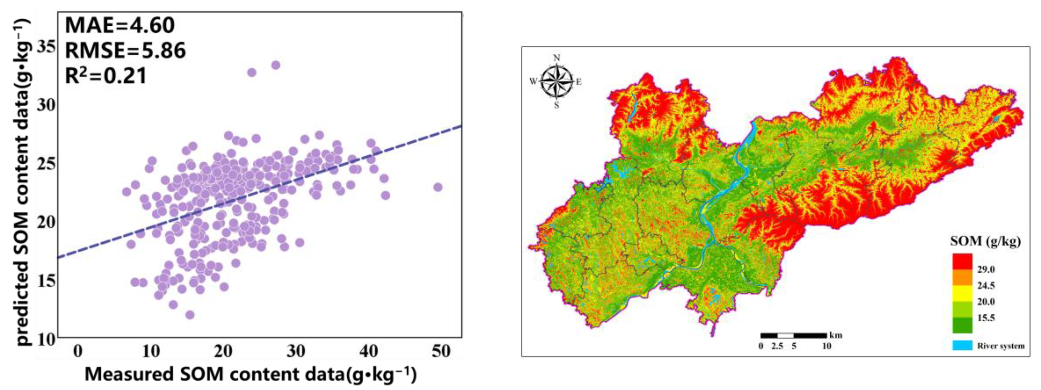
Figure 8.
Spatial distribution map of prediction accuracy of the RF-GA model for SOM.
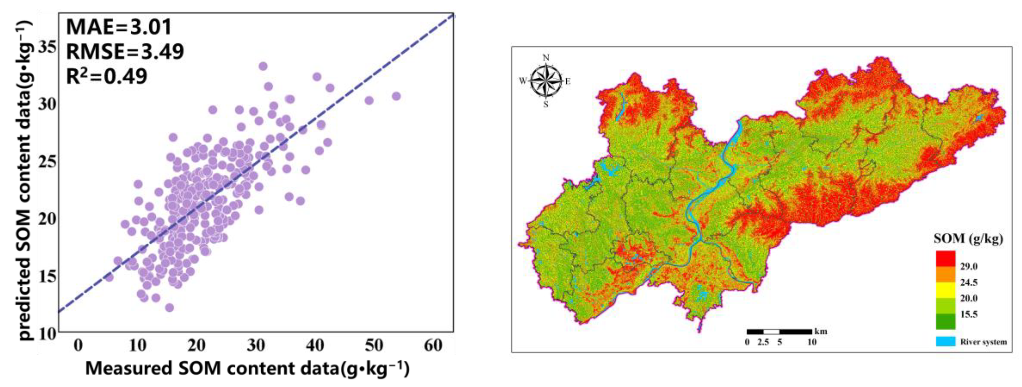

Table 1.
Input variables used in this study.
| Soil-Forming Factors | Input Variables | Spatial Resolution |
|---|---|---|
| Topographic factors | Analytical hillshading (AH), aspect (ASP), closed depressions (CDs), convergence index (CI), channel network base level (CNBL), channel network distance (CND), elevation (DEM), coefficient of variation of elevation (ECV), LS factor (LS), mass balance index (MBI), multiscale ridge top flatness (MRRTF), multi-resolution valley bottom flatness (MRVBF), plan curvature (PLC), profile curvature (PRC), relative slope position (RSP), surface cutting depth (SCD), slope (SLP), total catchment area (TCA), topographic position index (TPI), terrain ruggedness index (TRI), topographic wetness index (TWI), terrain undulation (TU), valley depth (VD), wind exposition index (WEI) | 12.5 m |
| Biological factors | Bare soil index (BSI), enhanced vegetation index (EVI), global environment monitoring index (GEMI), green normalized difference vegetation index (GNDVI), modified normalized difference water index (MNDWI), modified soil-adjusted vegetation index (MSAVI), normalized difference moisture index (NDMI), normalized difference vegetation index (NDVI), normalized difference water index (NDWI), net primary production (NPP), soil-adjusted vegetation index (SAVI), simple ratio (SR), visible light atmospheric impedance index (VARI) | 10 m |
| Soil texture | Sand content (sand), silt content (silt), clay content (clay) | 900 m |
| Climate factors | Evaporation (E_m), humidity mean (H_m), land surface temperature mean (LST_m), precipitation mean (P_m), temperature mean (T_m) | 1000 m |
| Land use (LU) | Vector data | |
| Soil type (ST) | ||
Table 2.
Band Information of Sentinel-2.
| Sentinel-2 Bands | Bandwidth (nm) | Central Wavelength (nm) |
|---|---|---|
| Band 1—coastal aerosol | 21 | 442.7 |
| Band 2—blue | 66 | 492.4 |
| Band 3—green | 36 | 559.8 |
| Band 4—red | 31 | 664.6 |
| Band 5—vegetation red edge | 2 | 704.1 |
| Band 6—vegetation red edge | 15 | 740.5 |
| Band 7—vegetation red edge | 20 | 782.8 |
| Band 8—NIR | 106 | 832.8 |
| Band 8A—narrow NIR | 21 | 864.7 |
| Band 9—water vapor | 20 | 945.1 |
| Band 10—SWR-Cirrus | 3 | 1373.5 |
| Band 11—SWIR | 91 | 1613.7 |
| Band 12—SWIR | 175 | 2202.4 |
Table 3.
Descriptive statistics of soil organic matter content at sampling points in the study area.
Table 3.
Descriptive statistics of soil organic matter content at sampling points in the study area.
| Type | Samples | Max (g·kg−1) |
Min (g·kg−1) |
AVE (g·kg−1) | SD (g·kg−1) | |
|---|---|---|---|---|---|---|
| Training set | Raw data | 1249 | 66.20 | 3.91 | 22.25 | 8.40 |
| Box–Cox | 1249 | 10.87 | 1.81 | 6.01 | 1.31 | |
| Validation set | Raw data | 311 | 58.60 | 5.21 | 22.50 | 8.58 |
| Box–Cox | 311 | 10.24 | 2.34 | 6.05 | 1.30 | |
| Type | CV (%) | Skewness | Kurtosis | K-S | ||
| Training set | Raw data | 37.77 | 0.85 | 1.89 | 0.000 | |
| Box–Cox | 21.84 | −0.01 | 0.44 | 0.081 | ||
| Validation set | Raw data | 38.15 | 0.86 | 1.40 | 0.006 | |
| Box–Cox | 21.54 | 0.12 | 0.29 | 0.200 | ||
Table 4.
Cross-validation results of different interpolation methods.
| Method | MAE | RMSE | R2 | LCCC |
|---|---|---|---|---|
| OK | 6.31 | 8.33 | 0.06 | 0.16 |
| RF | 4.60 | 5.86 | 0.21 | 0.38 |
| RF-GA | 3.02 | 3.49 | 0.49 | 0.67 |
Disclaimer/Publisher’s Note: The statements, opinions and data contained in all publications are solely those of the individual author(s) and contributor(s) and not of MDPI and/or the editor(s). MDPI and/or the editor(s) disclaim responsibility for any injury to people or property resulting from any ideas, methods, instructions or products referred to in the content. |
© 2025 by the authors. Licensee MDPI, Basel, Switzerland. This article is an open access article distributed under the terms and conditions of the Creative Commons Attribution (CC BY) license (http://creativecommons.org/licenses/by/4.0/).
Copyright: This open access article is published under a Creative Commons CC BY 4.0 license, which permit the free download, distribution, and reuse, provided that the author and preprint are cited in any reuse.


