Quantum Mechanics of the Timeon Field: Algebraic and Symplectic Framework for Quantum Gravity

1. Introduction

In conventional quantum field theory, the ontology is layered: there is a spacetime manifold with a prescribed metric, quantum fields living on that background, and a vacuum state defined in terms of those fields. Matter, vacuum, and gravitational behavior are treated as distinct ingredients of the theory. The approach developed in this paper starts from a different point of view. We posit a single complex scalar field, which we will call the timeon field, whose amplitude encodes a local time density and whose internal phase carries a $U\left(1\right)$ structure [1]. The central claim is that baryons are not independent elementary objects but stable composite configurations formed by the interaction between this time-density field and a conventional matter wavefunction. At the level of classical field theory, the timeon field $\Phi \left(x\right)$ is assumed to have a potential with at least two distinct minima:

• a metastable, low-density vacuum phase, and
• a deeper, condensed atomic phase.

Spatially localized regions of atomic phase embedded in the vacuum define finite-energy “lumps” of time density. When these lumps are coupled to an atomic matter wavefunction $\psi (\mathbf{x},t)$, they form what we call Baryon Partner States (BPS), in the tensor product Hilbert space:

$${\Psi }_{\mathrm{BPS}}\in {\mathcal{H}}_{\psi }\otimes {\mathcal{H}}_{\Phi }.$$

(1)

The purpose of this paper is to develop the full quantum mechanics of these BPS configurations and to show explicitly how familiar baryonic properties arise from the timeon field. We build upon the foundation of Chrono-Emergence and the Discrete-State Time Density (DTD) framework [2].

Baryon Partner States: Conceptual Overview

2. Composite Hilbert Space and Baryon Partner States

The first step toward a quantum description of baryons in the timeon framework is to formalize the joint Hilbert space on which both the matter wavefunction and the timeon field act. In this section we define the composite space, construct the corresponding Hamiltonian operators, and identify the Baryon Partner State (BPS) as a joint eigenstate of the full Hamiltonian.

2.1. Matter Sector: Wavefunction Hilbert Space

We begin with the standard Hilbert space for a single-particle (or effective single-particle) matter wavefunction,

$${\mathcal{H}}_{\psi }=L^2\left({\mathbb{R}}^3\right)=\left\{\psi :{\mathbb{R}}^3\to \mathbb{C}|\int {\left|\psi \left(\mathbf{x}\right)\right|}^2{\mathrm{d}}^{3}x<\infty \right\}.$$

(2)

The inner product is the usual

$$\langle {\psi }_1|{\psi }_2\rangle ={\int }_{{\mathbb{R}}^3}{\psi }_1^{*}\left(\mathbf{x}\right){\psi }_2\left(\mathbf{x}\right){\mathrm{d}}^{3}x.$$

(3)

The matter-sector Hamiltonian is written as

$$H_{\psi }=-{\displaystyle \frac{{\hslash }^2}{2m}}{\nabla }^2+U\left(\mathbf{x}\right),$$

(4)

where m is the bare matter mass parameter and $U\left(\mathbf{x}\right)$ a possible external potential. At this stage U plays no dynamical role; its purpose is to allow comparison with the usual Schrödinger picture [5]. All nontrivial interaction with the timeon field will enter through a separate interaction Hamiltonian.

2.2. Timeon Sector: Field Configuration Space

The timeon field is a complex scalar function,

$$\Phi \left(\mathbf{x}\right)=\widehat{t}\left(\mathbf{x}\right)e^{i\theta \left(\mathbf{x}\right)},$$

(5)

with amplitude $\widehat{t}\ge 0$ encoding local time density and phase $\theta$ encoding an internal $U\left(1\right)$ degree of freedom. Before introducing dynamics (which will come in Section 3), we specify the kinematic Hilbert space ${\mathcal{H}}_{\Phi }$ as the space of square-integrable wavefunctionals over field configurations:

$${\mathcal{H}}_{\Phi }=L^2\left({\mathcal{C}}_{\Phi },\mathcal{D}\Phi \right),$$

(6)

where ${\mathcal{C}}_{\Phi }$ is the configuration space of complex fields and $\mathcal{D}\Phi$ is the formal functional measure. A generic state in this sector is written

$${\Psi }_{\Phi }[\Phi \left(·\right)],$$

(7)

a functional of the spatial profile of the timeon field. For classical field configurations, expectation values will later be dominated by stationary-phase contributions corresponding to finite-energy configurations of $\Phi$. The timeon-sector Hamiltonian will be developed fully in Section 3. For now, we denote it symbolically by

$$H_{\Phi }[\Phi ,-i\hslash \delta /\delta \Phi ],$$

(8)

emphasizing that it acts on functionals of the field.

2.3. Composite Hilbert Space

The system consisting of matter and timeon field is described on the tensor-product Hilbert space [4]

$$\mathcal{H}={\mathcal{H}}_{\psi }\otimes {\mathcal{H}}_{\Phi }.$$

(9)

A general state has the form

$$\Psi (\mathbf{x},\Phi )=\psi \left(\mathbf{x}\right)\otimes {\Psi }_{\Phi }[\Phi ]+\sum _i{c}_i{\psi }_i\left(\mathbf{x}\right)\otimes {\Psi }_{\Phi ,i}[\Phi ]+\dots ,$$

(10)

but for physical baryons we will be concerned with states that are approximately separable into a localized matter wavefunction and a localized timeon configuration. The inner product on $\mathcal{H}$ factorizes:

$$\langle {\Psi }_1|{\Psi }_2\rangle ={\langle {\psi }_1|{\psi }_2\rangle }_{\psi }{\langle {\Psi }_{\Phi ,1}|{\Psi }_{\Phi ,2}\rangle }_{\Phi }.$$

(11)

2.4. Composite Hamiltonian

The dynamics of the joint system are governed by a Hamiltonian of the form

$$H=H_{\psi }\otimes {\mathbb{I}}_{\Phi }+{\mathbb{I}}_{\psi }\otimes H_{\Phi }+H_{\mathrm{int}},$$

(12)

where:

• $H_{\psi }$ acts only on the matter wavefunction,
• $H_{\Phi }$ acts only on the timeon sector, and
• $H_{\mathrm{int}}$ couples them locally.

To anticipate later developments, the interaction Hamiltonian will take the form

$$H_{\mathrm{int}}=g\int {\mathrm{d}}^3{x\left|\psi \left(\mathbf{x}\right)\right|}^2{|\Phi \left(\mathbf{x}\right)|}^2,$$

(13)

where g is a coupling constant. This term expresses the intuitive fact that high matter probability density tends to “compress” the timeon field toward high-amplitude (atomic) configurations. Likewise, a region in which the timeon field has adopted the atomic phase produces an effective potential for the matter wavefunction. In classical field realizations, the operator ${|\Phi |}^2$ becomes simply the squared amplitude ${\widehat{t}}^2\left(\mathbf{x}\right)$; when quantized, it acts as a local operator multiplying the wavefunctional ${\Psi }_{\Phi }$.

2.5. Definition of the Baryon Partner State

We now define the key object of the theory: the Baryon Partner State (BPS). A BPS is a joint eigenstate of the composite Hamiltonian (12) of the form

$${\Psi }_{\mathrm{BPS}}={\psi }_{\mathrm{BPS}}\left(\mathbf{x}\right)\otimes {\Psi }_{\Phi ,\mathrm{BPS}}[\Phi ],$$

(14)

such that

$$H{\Psi }_{\mathrm{BPS}}=E_{\mathrm{BPS}}{\Psi }_{\mathrm{BPS}}.$$

(15)

The eigenvalue $E_{\mathrm{BPS}}$ defines the effective mass of the composite object,

$$m_{\mathrm{BPS}}={\displaystyle \frac{E_{\mathrm{BPS}}}{c^2}},$$

(16)

and the structure of ${\Psi }_{\Phi ,\mathrm{BPS}}$ determines the internal charge and stability properties. The BPS must satisfy three physical conditions:

1.

Finite energy: the timeon configuration must minimize $H_{\Phi }$ subject to boundary conditions (derived in Section 4).

2.

Self-consistency: the matter wavefunction ${\psi }_{\mathrm{BPS}}$ must be bound to the timeon configuration that it helps generate.

3.

Locality: both ${\psi }_{\mathrm{BPS}}$ and ${\Psi }_{\Phi ,\mathrm{BPS}}$ must be spatially localized, yielding a finite, well-defined composite excitation.

These conditions distinguish BPS configurations from arbitrary fluctuations of either field sector. Only when the interaction term (13) is included do localized atomic-phase solutions of the timeon field become stable, and only then does the matter wavefunction acquire a localized, baryon-like structure.

2.6. Remarks on Separability and Entanglement

While the idealized definition above uses a separable tensor product state $\psi \otimes {\Psi }_{\Phi }$, the physical BPS is generally entangled. The presence of the interaction Hamiltonian implies that the true ground-state solution takes the form

$${\Psi }_{\mathrm{BPS}}(\mathbf{x},\Phi )=\sum _i{c}_i{\psi }_i\left(\mathbf{x}\right)\otimes {\Psi }_{\Phi ,i}[\Phi ],$$

(17)

with coefficients $c_i$ determined by minimizing the total energy functional. The separable form is therefore best understood as the leading-order description in a Born–Oppenheimer-like approximation [6] in which the timeon field provides a slowly varying background for the matter wavefunction. This structure will be made explicit in later sections, where we derive both the static timeon configurations and the coupled evolution equations for $\psi$ and $\Phi$.

3. Timeon Field Theory: Lagrangian, Hamiltonian, and Phase Structure

We now construct the timeon field theory that governs the time-density field introduced in the previous section. The timeon is treated as a complex scalar field,

$$\Phi \left(x\right)=\widehat{t}\left(x\right)e^{i\theta \left(x\right)},$$

(18)

with amplitude $\widehat{t}\ge 0$ capturing local time density and phase $\theta$ carrying an internal $U\left(1\right)$ structure. Throughout we use the four-vector notation $x^{\mu }=(ct,\mathbf{x})$ and the metric signature $(+,-,-,-)$. The goal of this section is to build the complete field-theoretic framework: the Lagrangian density, Euler–Lagrange equations, Hamiltonian density, and the potential structure that supports vacuum and atomic phases.

3.1. Lagrangian Density

We adopt a physical Lagrangian density scaled by a stiffness modulus $Z_t$ (units of Force) to ensure the scalar field yields units of Energy Density:

$${\mathcal{L}}_{\Phi }={\displaystyle \frac{Z_t}{2}}\left[{\left({\partial }_{\mu }\widehat{t}\right)}^2+{\widehat{t}}^2{\left({\partial }_{\mu }\theta \right)}^2\right]-V\left({\widehat{t}}^2\right).$$

(19)

Here, the amplitude field $\widehat{t}$ has units of time-density ($s/m$) and $Z_t$ provides the necessary conversion to Joules/$m^3$.

The two degrees of freedom are thus:

• $\widehat{t}$: a real amplitude field controlling time-density,
• $\theta$: a Goldstone-like phase variable.

We will see that stable baryonic configurations arise primarily from nonlinear structure in V and localized gradients in $\widehat{t}$.

3.2. Euler–Lagrange Equations

The Euler–Lagrange equation for the complex field is:

$${\partial }_{\mu }\left({\displaystyle \frac{\partial {\mathcal{L}}_{\Phi }}{\partial \left({\partial }_{\mu }{\Phi }^{*}\right)}}\right)-{\displaystyle \frac{\partial {\mathcal{L}}_{\Phi }}{\partial {\Phi }^{*}}}=0.$$

(20)

Working directly with $\Phi$ yields the d’Alembertian dynamics [5]:

$$\square \Phi +{\displaystyle \frac{\partial V}{\partial {\Phi }^{*}}}=0,$$

(21)

where $\square ={\partial }_{\mu }{\partial }^{\mu }$ is the d’Alembertian. Alternatively, in amplitude/phase variables:

• Amplitude equation:

$$\square \widehat{t}-\widehat{t}{\left({\partial }_{\mu }\theta \right)}^2+{\displaystyle \frac{1}{2}}{V}^{\prime }\left({\widehat{t}}^2\right)\left(2\widehat{t}\right)=0,$$

(22)

where $V^{\prime }$ denotes derivative with respect to its argument $\left({\widehat{t}}^2\right)$.

• Phase equation:

$${\partial }_{\mu }\left({\widehat{t}}^2{\partial }^{\mu }\theta \right)=0.$$

(23)

The phase equation expresses the local conservation of a $U\left(1\right)$-like current,

$$j^{\mu }={\widehat{t}}^2{\partial }^{\mu }\theta ,$$

(24)

which is the Noether current [7] that will play a role in defining effective “charge” of BPS solutions.

3.3. Hamiltonian Density

To compute energies of static configurations (including BPS cores) we require the Hamiltonian density. For a complex scalar,

$${\mathcal{H}}_{\Phi }=|{\pi }_{\Phi }{|}^2+{|\nabla \Phi |}^2+{V\left(\right|\Phi |}^2),$$

(25)

where the canonical momentum is

$${\pi }_{\Phi }={\displaystyle \frac{\partial {\mathcal{L}}_{\Phi }}{\partial \left({\partial }_t{\Phi }^{*}\right)}}=\dot{\Phi }.$$

(26)

Thus explicitly,

$${\mathcal{H}}_{\Phi }=|\dot{\Phi }{|}^2+{|\nabla \Phi |}^2+{V\left(\right|\Phi |}^2).$$

(27)

In polar form:

$${|\nabla \Phi |}^2={(\nabla \widehat{t})}^2+{\widehat{t}}^2{(\nabla \theta )}^2,$$

(28)

and

$$|\dot{\Phi }{|}^2={\left(\dot{\widehat{t}}\right)}^2+{\widehat{t}}^2{\left(\dot{\theta }\right)}^2.$$

(29)

For static solutions (all BPS cores considered here), $\dot{\widehat{t}}=0$ and $\dot{\theta }=0$, yielding the static Hamiltonian density:

$$\begin{array}{|c|}\hline {\mathcal{H}}_{\Phi }^{\mathrm{static}}={(\nabla \widehat{t})}^2+{\widehat{t}}^2{(\nabla \theta )}^2+V\left({\widehat{t}}^2\right).\\ \hline\end{array}$$

(30)

This is the expression we will minimize to obtain baryon-like solutions.

3.4. Double-Well Potential and Phase Structure

To support baryon-like localized lumps, the potential must have at least two distinct minima:

$$V\left({\widehat{t}}^2\right)=\lambda {({\widehat{t}}^2-v_{\mathrm{vac}}^2)}^2{({\widehat{t}}^2-v_{\mathrm{atom}}^2)}^2,$$

(31)

with $v_{\mathrm{atom}}>v_{\mathrm{vac}}\ge 0$. The minima occur at $\widehat{t}=v_{\mathrm{vac}}$ and $\widehat{t}=v_{\mathrm{atom}}$. We refer to these as:

• Vacuum phase:$\widehat{t}=v_{\mathrm{vac}}$ (low time density)
• Atomic phase:$\widehat{t}=v_{\mathrm{atom}}$ (Condensed Lattice Phase)

Figure 1. The Timeon Lattice Potential (TLP). The potential energy density $V\left(\widehat{t}\right)$ features a metastable Vacuum basin and a stable Atomic well. Baryon Partner State formation corresponds to tunneling through the barrier separating these phases. Scope of this plot: This theoretical landscape is restricted to the formation of discrete Baryon Partner States and intentionally excludes black hole interiors and chrono-shear events (i.e., dense- and shear-time–density phases).

Figure 1. The Timeon Lattice Potential (TLP). The potential energy density $V\left(\widehat{t}\right)$ features a metastable Vacuum basin and a stable Atomic well. Baryon Partner State formation corresponds to tunneling through the barrier separating these phases. Scope of this plot: This theoretical landscape is restricted to the formation of discrete Baryon Partner States and intentionally excludes black hole interiors and chrono-shear events (i.e., dense- and shear-time–density phases).

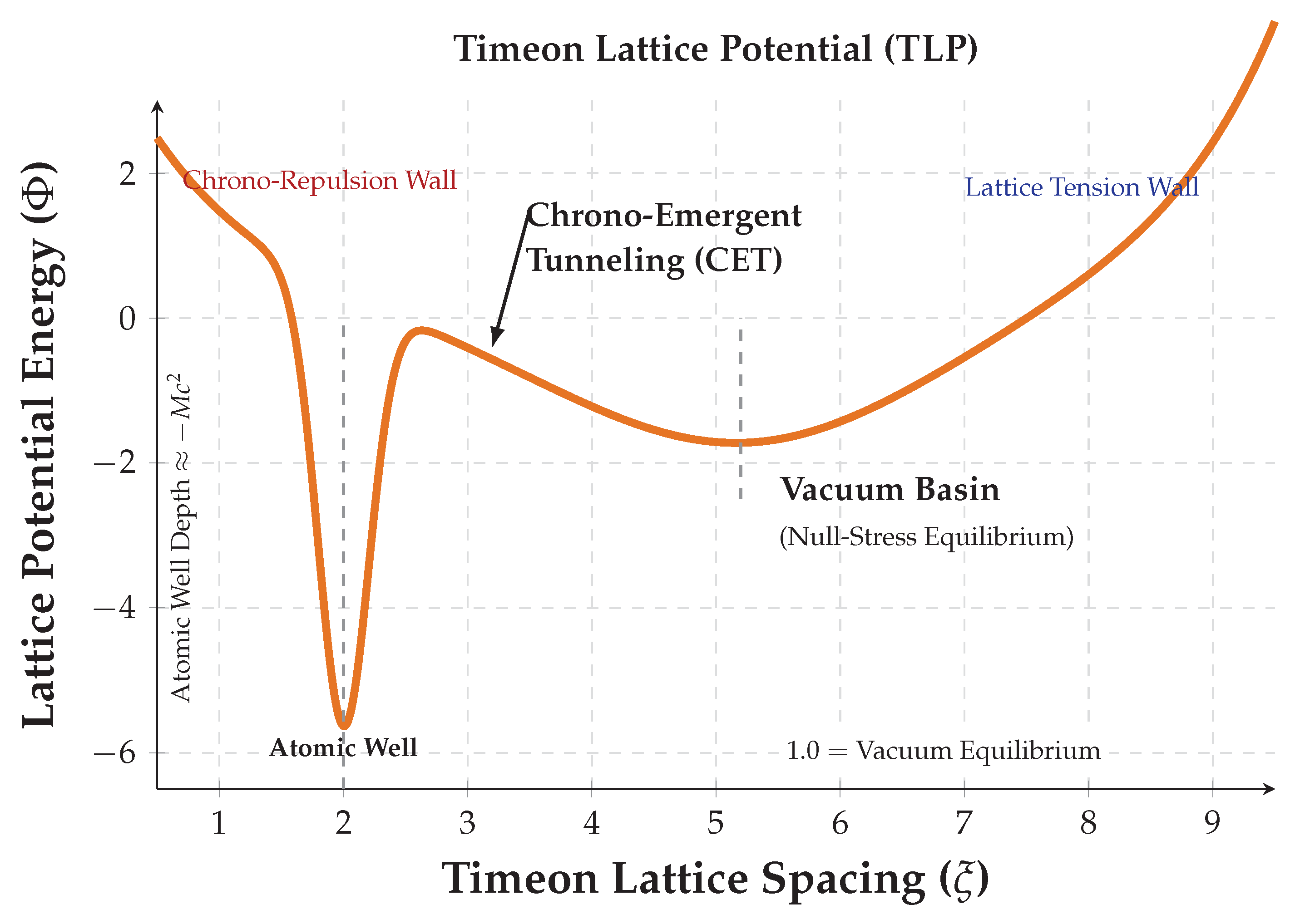
The barrier separating them determines tunneling rates and bubble nucleation structure.

Quadratic expansion and mass scales

Expanding around each minimum yields the small-oscillation mass:

- Around vacuum phase:

$$\begin{array}{cc}\hfill \widehat{t}\left(x\right)& =v_{\mathrm{vac}}+\delta t\left(x\right),\hfill \end{array}$$

(32)

$$\begin{array}{cc}\hfill m_{\mathrm{vac}}^2& ={\left.{\displaystyle \frac{{\mathrm{d}}^{2}V}{\mathrm{d}{\widehat{t}}^2}}\right|}_{\widehat{t}=v_{\mathrm{vac}}}.\hfill \end{array}$$

(33)

- Around atomic phase:

$$\begin{array}{cc}\hfill \widehat{t}\left(x\right)& =v_{\mathrm{atom}}+\delta t\left(x\right),\hfill \end{array}$$

(34)

$$\begin{array}{cc}\hfill m_{\mathrm{atom}}^2& ={\left.{\displaystyle \frac{{\mathrm{d}}^{2}V}{\mathrm{d}{\widehat{t}}^2}}\right|}_{\widehat{t}=v_{\mathrm{atom}}}.\hfill \end{array}$$

(35)

Both masses will appear later in the fluctuation spectrum of BPS cores.

3.5. Energetics of Phase Boundaries

Finite-energy static solutions require that $\widehat{t}$ interpolate between different minima over a finite spatial width. The energy per unit area of such an interface (“domain wall”) is

$$\sigma ={\int }_{v_{\mathrm{vac}}}^{v_{\mathrm{atom}}}\mathrm{d}\widehat{t}\sqrt{2V\left({\widehat{t}}^2\right)}.$$

(36)

This quantity plays a central role in critical-radius calculations, bubble nucleation barriers, and BPS core stability. We will use $\sigma$ in Section 4 and Section 5 to derive baryon mass and tunneling thresholds.

3.6. Summary of Key Results from Section 3

• The timeon field is governed by the Lagrangian (19) and Hamiltonian density (30).
• The potential must have at least two minima, leading to vacuum and atomic phases.
• Domain walls have finite surface tension $\sigma$ given by (36).
• The small-oscillation masses in each phase determine the reconfiguration spectrum of baryons.

The next section constructs explicit finite-energy static solutions representing Baryon Partner States.

4. Static Baryon Partner State (BPS) Solutions

We now derive the finite-energy, static configurations of the timeon field that correspond to Baryon Partner States (BPS). These solutions represent localized regions of atomic phase embedded within the vacuum phase, stabilized by the nonlinear structure of the potential and, later (Section 6), by coupling to the matter wavefunction. The goal of this section is to obtain the radial profile of a static BPS, its energy, and its effective charge, and to establish the topological reasons why such configurations cannot decompose into smaller constituents.

4.1. Spherical Ansatz

Because baryons are experimentally observed to be approximately spherically symmetric in their lowest-energy state, we impose spherical symmetry on the static timeon configuration:

$$\Phi \left(\mathbf{x}\right)=\widehat{t}\left(r\right)e^{i\theta \left(r\right)},$$

(37)

where $r=\left|\mathbf{x}\right|$. Staticity implies ${\partial }_t\widehat{t}=0$ and ${\partial }_t\theta =0$. Thus only spatial gradients contribute to the energy. Under spherical symmetry:

$${|\nabla \Phi |}^2={\left({\partial }_r\widehat{t}\right)}^2+{\widehat{t}}^2{\left({\partial }_r\theta \right)}^2.$$

(38)

The static energy functional from (30) becomes:

$$E[\widehat{t},\theta ]=4\pi {\int }_0^{\infty }{r}^2\left[{\left({\widehat{t}}^{\prime }\right)}^2+{\widehat{t}}^2{\left({\theta }^{\prime }\right)}^2+V\left({\widehat{t}}^2\right)\right]\mathrm{d}r,$$

(39)

where primes denote derivatives with respect to r.

4.2. Boundary Conditions

Finite-energy solutions require:

1.

Core condition: The field must approach the atomic phase at $r=0$,

$$\widehat{t}\left(0\right)=v_{\mathrm{atom}},{\theta }^{\prime }\left(0\right)=0.$$

2.

Vacuum exterior: At large r the field returns to the vacuum phase:

$$\widehat{t}(r\to \infty )=v_{\mathrm{vac}}.$$

3.

Finite energy: The phase gradient must vanish outside the core,

$${\theta }^{\prime }(r\to \infty )=0.$$

4.

Regularity at $r=0$: Terms like $r^{-2}$ must not diverge, implying

$${\widehat{t}}^{\prime }\left(0\right)=0,\theta \left(0\right)=\mathrm{finite}.$$

These conditions uniquely determine the qualitative shape of a BPS profile.

4.3. Radial Field Equations

Variation of the energy functional (39) yields the coupled radial Euler–Lagrange equations [5].

• Amplitude equation:

$${\widehat{t}}^{″}+{\displaystyle \frac{2}{r}}{\widehat{t}}^{\prime }-\widehat{t}{\left({\theta }^{\prime }\right)}^2-{\displaystyle \frac{1}{2}}{V}^{\prime }\left({\widehat{t}}^2\right)\left(2\widehat{t}\right)=0,$$

(40)

• Phase equation:

$${\displaystyle \frac{\mathrm{d}}{\mathrm{d}r}}\left(r^2{\widehat{t}}^2{\theta }^{\prime }\right)=0.$$

(41)

Integrating the phase equation:

$$r^2{\widehat{t}}^2{\theta }^{\prime }=Q,$$

(42)

where Q is a constant of integration. This constant behaves as a conserved topological charge associated with phase gradients in the timeon field. Thus:

$${\theta }^{\prime }\left(r\right)={\displaystyle \frac{Q}{r^2\widehat{t}{\left(r\right)}^2}}.$$

(43)

Substituting back into (40) yields the single radial equation:

$${\widehat{t}}^{″}+{\displaystyle \frac{2}{r}}{\widehat{t}}^{\prime }-{\displaystyle \frac{Q^2}{r^4{\widehat{t}}^3}}-V^{\prime }\left({\widehat{t}}^2\right)\widehat{t}=0.$$

(44)

This nonlinear ODE defines the full static BPS profile.

4.4. Interpretation of the Charge Parameter Q

The quantity Q controls the strength of the phase gradient in the core region. Several key properties follow:

• If $Q=0$, the phase is constant and the solution has no internal $U\left(1\right)$ excitation. This describes a neutral baryon-like configuration.
• If $Q\ne 0$, the core hosts a localized winding of the phase, contributing to a finite $U\left(1\right)$ charge density:

  $$j^r={\widehat{t}}^2{\theta }^{\prime }.$$
• Because the energy density contains

  $${\widehat{t}}^2{\left({\theta }^{\prime }\right)}^2={\displaystyle \frac{Q^2}{r^4{\widehat{t}}^2}},$$

  the charge is confined to regions where $\widehat{t}$ is large (atomic phase). This provides a direct algebraic mechanism for baryonic charge confinement.

4.5. Energy of a BPS Configuration

Substituting (43) into the static energy functional yields:

$$E_{\mathrm{BPS}}=4\pi {\int }_0^{\infty }{r}^2\left[{\left({\widehat{t}}^{\prime }\right)}^2+{\displaystyle \frac{Q^2}{r^4{\widehat{t}}^2}}+V\left({\widehat{t}}^2\right)\right]\mathrm{d}r.$$

(45)

Three competing contributions determine the radius and stability of a BPS:

1.

Gradient energy: favors slowly varying $\widehat{t}$.

2.

Phase-gradient energy (charge term): grows rapidly as $\widehat{t}\to 0$, confining charge to the atomic-phase core.

3.

Potential energy: favors either vacuum or atomic phase in bulk.

Balancing these terms yields a stable finite-radius atomic-phase bubble.

4.6. Thin-Wall Approximation

When the energy barrier between vacuum and atomic phase is large relative to gradient contributions, the BPS resembles a domain-wall bubble of radius R. In this regime we approximate:

$$\widehat{t}\left(r\right)\approx \left\{\begin{array}{cc}{v}_{\mathrm{atom}},\hfill & r<R,\hfill \\ v_{\mathrm{vac}},\hfill & r>R,\hfill \end{array}\right.\mathrm{with}\mathrm{a}\mathrm{narrow}\mathrm{transition}\mathrm{of}\mathrm{width}\delta \ll R.$$

The energy simplifies to:

$$E_{\mathrm{BPS}}\left(R\right)=4\pi R^2\sigma +{\displaystyle \frac{4\pi Q^2}{v_{\mathrm{atom}}^{2}R}}+{\displaystyle \frac{4\pi }{3}}{R}^3\Delta V,$$

(46)

where $\Delta V=V\left(v_{\mathrm{atom}}^2\right)-V\left(v_{\mathrm{vac}}^2\right)<0$. Minimizing (46) gives the equilibrium BPS radius:

$${\displaystyle \frac{\mathrm{d}E}{\mathrm{d}R}}=0\Rightarrow 8\pi R\sigma -{\displaystyle \frac{4\pi Q^2}{v_{\mathrm{atom}}^2{R}^2}}+4\pi R^2\Delta V=0.$$

(47)

This cubic equation determines the physical radius as a function of charge Q, potential parameters, and surface tension.

4.7. Topological Stability and Confinement

The BPS core is topologically protected by the structure of the phase variable $\theta$ and by the requirement that $\widehat{t}$ remain nonzero inside the atomic region. Key features:

• The phase equation mandates that $r^2{\widehat{t}}^2{\theta }^{\prime }=Q$. If one attempted to split a BPS into smaller charged fragments, this relation would require singularities (where $\widehat{t}=0$) to maintain total Q. Such configurations have infinite energy.
• The volume energy density difference $\Delta V<0$ favors a stable core of atomic phase.
• The gradient term penalizes fragmentation because multiple small bubbles have larger total surface area than a single bubble of the same volume.

Thus the BPS is intrinsically confined: it cannot decompose without energy divergence or violation of charge conservation.

4.8. Summary of Section 4

We have:

• Written the full radial equations for static timeon configurations.
• Identified the conserved charge Q associated with phase gradients.
• Derived the energy functional for BPS solutions.
• Obtained approximate analytic behavior via the thin-wall limit.
• Shown that confinement follows directly from the algebraic and topological structure of the timeon field.

These results prepare the ground for computing tunneling, bubble formation, and BPS nucleation in the next section.

5. Vacuum-to-Atomic Tunneling and Bubble Nucleation

In the previous section we constructed static Baryon Partner State configurations by minimizing the energy functional. We now consider the opposite question: How does a localized region of atomic phase form dynamically within the vacuum? The answer requires a tunneling calculation in which the timeon field transitions from the vacuum minimum to the atomic minimum through a Euclidean “bounce” solution. This section develops the complete quantum tunneling formalism for the timeon field, derives the critical radius for bubble nucleation, and identifies the tunneling exponent governing BPS formation.

5.1. Euclidean Action for the Timeon Field

Quantum tunneling in scalar field theory is governed by the Euclidean action, obtained by Wick rotation $t\to -i\tau$ [11]:

$$S_E[\Phi ]=\int \mathrm{d}\tau {\mathrm{d}}^{3}x\left[|{\partial }_{\tau }{\Phi |}^2+{|\nabla \Phi |}^2+{V\left(\right|\Phi |}^2)\right].$$

(48)

For tunneling from the vacuum to the atomic phase, the relevant solutions possess $O\left(4\right)$ symmetry in the Euclidean coordinates

$${\rho }^2={\tau }^2+r^2,$$

(49)

leading to the ansatz

$$\Phi \left(\rho \right)=\widehat{t}\left(\rho \right)e^{i\theta \left(\rho \right)}.$$

(50)

The Euclidean action becomes

$$S_E[\widehat{t},\theta ]=2{\pi }^2{\int }_0^{\infty }{\rho }^3\left[{\left({\widehat{t}}^{\prime }\right)}^2+{\widehat{t}}^2{\left({\theta }^{\prime }\right)}^2+V\left({\widehat{t}}^2\right)\right]\mathrm{d}\rho .$$

(51)

5.2. Euclidean Field Equations

The Euler–Lagrange equations corresponding to (51) are:

Amplitude:

$${\widehat{t}}^{″}+{\displaystyle \frac{3}{\rho }}{\widehat{t}}^{\prime }-\widehat{t}{\left({\theta }^{\prime }\right)}^2-V^{\prime }\left({\widehat{t}}^2\right)\widehat{t}=0.$$

(52)

Phase:

$${\displaystyle \frac{\mathrm{d}}{\mathrm{d}\rho }}\left({\rho }^3{\widehat{t}}^2{\theta }^{\prime }\right)=0.$$

(53)

Integrating:

$${\rho }^3{\widehat{t}}^2{\theta }^{\prime }=Q_E,$$

(54)

where $Q_E$ is a Euclidean analogue of the charge parameter. Most tunneling calculations assume $Q_E=0$, corresponding to a phase-uniform bounce. We will treat this case first, then include nonzero charge.

5.3. Bounce Solution for $Q_E=0$

With ${\theta }^{\prime }=0$, the Euclidean equation reduces to:

$${\widehat{t}}^{″}+{\displaystyle \frac{3}{\rho }}{\widehat{t}}^{\prime }-V^{\prime }\left({\widehat{t}}^2\right)\widehat{t}=0.$$

(55)

Boundary conditions:

$$\begin{array}{cc}\hfill & {\widehat{t}}^{\prime }\left(0\right)=0,\hfill \end{array}$$

(56)

$$\begin{array}{cc}\hfill & \widehat{t}(\rho \to \infty )=v_{\mathrm{vac}}.\hfill \end{array}$$

(57)

The solution interpolates from the atomic minimum near $\rho =0$ to the vacuum minimum as $\rho \to \infty$. The configuration is called the bounce and denoted ${\widehat{t}}_B\left(\rho \right)$ [12]. The tunneling exponent is:

$$B=S_E\left[{\widehat{t}}_B\right]-S_E\left[{\widehat{t}}_{\mathrm{vac}}\right].$$

(58)

The nucleation rate per unit volume is:

$$\Gamma /V\sim A{e}^{-B/\hslash },$$

(59)

where A is a fluctuation determinant prefactor.

5.4. Thin-Wall Limit and Critical Bubble Radius

When the barrier separating the two minima is large compared to their energy difference, the bounce resembles a thin-walled bubble. In this limit, the Euclidean action reduces to:

$$S_E\left(R\right)=2{\pi }^2{R}^3\sigma -{\displaystyle \frac{{\pi }^2}{2}}{R}^4\Delta V,$$

(60)

where:

• $\sigma$ is the surface tension from (36),
• $\Delta V=V\left(v_{\mathrm{atom}}^2\right)-V\left(v_{\mathrm{vac}}^2\right)<0$.

Differentiating:

$${\displaystyle \frac{\mathrm{d}{S}_E}{\mathrm{d}R}}=6{\pi }^2{R}^2\sigma -2{\pi }^2{R}^3\Delta V=0,$$

(61)

leading to the critical radius:

$$R_c={\displaystyle \frac{3\sigma }{|\Delta V|}}.$$

(62)

Only bubbles with $R\ge R_c$ expand; smaller bubbles collapse. Substituting back:

$$B_{\mathrm{thin}}={\displaystyle \frac{27{\pi }^2{\sigma }^4}{{2|\Delta V|}^3}}.$$

(63)

This closed-form expression is crucial to estimating BPS nucleation probabilities.

5.5. Effect of Nonzero Charge $Q_E$

If $Q_E\ne 0$, the Euclidean phase gradient contributes a centrifugal-like term:

$${\widehat{t}}^2{\left({\theta }^{\prime }\right)}^2={\displaystyle \frac{Q_E^2}{{\rho }^6{\widehat{t}}^2}}.$$

(64)

This term:

• suppresses configurations where $\widehat{t}$ is small,
• drives the interior of the bubble toward the atomic phase,
• increases the effective surface pressure,
• decreases the tunneling exponent B.

The corrected thin-wall action becomes:

$$S_E\left(R\right)=2{\pi }^2{R}^3\sigma -{\displaystyle \frac{{\pi }^2}{2}}{R}^4\Delta V+{\displaystyle \frac{C{Q}_E^2}{R^2{v}_{\mathrm{atom}}^2}},$$

(65)

where C is an order-one geometric constant. Minimizing yields a modified critical radius:

$$R_c\left(Q_E\right)\approx \left({\displaystyle \frac{3\sigma }{|\Delta V|}}+{\displaystyle \frac{Q_E^2}{3{\pi }^2{v}_{\mathrm{atom}}^2\sigma }}\right)+\mathcal{O}\left(Q_E^4\right).$$

(66)

Thus: - charge slightly expands the critical radius, - but makes the atomic phase more energetically favored inside the bubble, - and typically decreases the tunneling exponent. Charged tunneling therefore increases the likelihood of BPS formation.

5.6. Interpretation: Matter Formation via Timeon Tunneling

A physically transparent interpretation emerges:

1.

The vacuum phase is metastable.

2.

Quantum fluctuations occasionally nucleate a small region of atomic phase.

3.

If the region exceeds the critical radius $R_c$, it expands.

4.

The presence of matter (Section 6) reduces $R_c$ locally by compressing the timeon field.

5.

The expanding atomic region forms the core of a BPS.

Thus baryon formation is not simply imposed—it is a dynamical outcome of timeon-field tunneling stabilized by matter-wave coupling.

5.7. Summary of Section 5

We have:

• Formulated vacuum-to-atomic tunneling using the Euclidean action.
• Derived the bounce equations and boundary conditions.
• Obtained the critical radius $R_c$ and tunneling exponent B.
• Extended the thin-wall approximation to include charge.
• Established the mechanism by which atomic-phase bubbles become stabilized baryonic cores.

The next section introduces the coupling to the matter wavefunction, completing the dynamical picture of Baryon Partner States.

6. Coupling to the Matter Wavefunction and Self-Consistent Dynamics

Up to this point, the timeon field has been treated independently of the matter wavefunction. We now introduce the essential ingredient of the theory: a local interaction between the matter density ${\left|\psi \right|}^2$ and the timeon amplitude ${\widehat{t}}^2$. This coupling allows high matter density to “compress” the timeon field toward the atomic phase, reducing the tunneling barrier and stabilizing Baryon Partner States (BPS). Conversely, the timeon configuration modifies the effective potential seen by the matter wavefunction, binding $\psi$ to the atomic core it helps generate. The result is a fully self-consistent system where matter and timeon fields mutually determine each other’s configuration.

6.1. Interaction Hamiltonian

We postulate the simplest local, scalar, bilinear interaction:

$$H_{\mathrm{int}}=g\int {\mathrm{d}}^3{x\left|\psi (\mathbf{x},t)\right|}^2{|\Phi (\mathbf{x},t)|}^2,$$

(67)

where g is a real coupling constant controlling the strength of the compression effect. Writing $\Phi =\widehat{t}{e}^{i\theta }$:

$${|\Phi |}^2={\widehat{t}}^2.$$

Thus the interaction term becomes:

$$H_{\mathrm{int}}=g\int {\mathrm{d}}^{3}x{\left|\psi \right|}^2{\widehat{t}}^2.$$

(68)

This is the lowest-order operator capable of:

• lowering the effective potential seen by $\widehat{t}$ in regions where ${\left|\psi \right|}^2$ is large,
• raising the effective potential of $\psi$ in regions where $\widehat{t}$ is small,
• and creating a self-localizing composite eigenstate.

The interaction is local, Hermitian, and preserves all global symmetries.

6.2. Total Hamiltonian and Equations of Motion

The full Hamiltonian is:

$$H=H_{\psi }+H_{\Phi }+H_{\mathrm{int}},$$

(69)

with $H_{\psi }$ and $H_{\Phi }$ defined in earlier sections. We now derive the equations governing the coupled dynamics.

6.2.1. Matter Wavefunction Equation

Varying the total action with respect to ${\psi }^{*}$ yields:

$$i\hslash {\displaystyle \frac{\partial \psi }{\partial t}}=\left[-{\displaystyle \frac{{\hslash }^2}{2m}}{\nabla }^2+U\left(\mathbf{x}\right)+g{\widehat{t}}^2(\mathbf{x},t)\right]\psi .$$

(70)

Thus the timeon amplitude ${\widehat{t}}^2$ contributes an effective potential:

$$U_{\mathrm{eff}}\left(\mathbf{x}\right)=U\left(\mathbf{x}\right)+g{\widehat{t}}^2\left(\mathbf{x}\right).$$

(71)

Regions of high $\widehat{t}$ (atomic phase) attract the matter wavefunction, creating a stable bound state. This is the coupled Schrödinger equation [5].

6.2.2. Timeon Amplitude Equation

Varying the total action with respect to $\widehat{t}$ yields:

$$\square \widehat{t}-\widehat{t}{\left({\partial }_{\mu }\theta \right)}^2+V^{\prime }\left({\widehat{t}}^2\right)\widehat{t}=-g{\left|\psi \right|}^2\widehat{t}.$$

(72)

The right-hand side shows explicitly: - matter density suppresses the vacuum minimum, - and deepens the atomic minimum, - effectively tilting the potential energy in favor of the atomic phase. More precisely, the interaction modifies the potential:

$$V_{\mathrm{eff}}\left({\widehat{t}}^2\right)=V\left({\widehat{t}}^2\right)+g{\left|\psi \right|}^2{\widehat{t}}^2.$$

Thus: - if $g>0$: matter pushes the timeon field to larger amplitudes (atomic phase), - if $g<0$: matter repels the atomic phase (we focus on $g>0$).

6.2.3. Timeon Phase Equation

Variation with respect to $\theta$ yields the modified current conservation equation:

$${\partial }_{\mu }\left({\widehat{t}}^2{\partial }^{\mu }\theta \right)=0.$$

(73)

Because $H_{\mathrm{int}}$ depends only on ${\widehat{t}}^2$, the $U\left(1\right)$ phase remains a conserved degree of freedom. The associated charge Q remains valid in the presence of matter.

6.3. Self-Consistent BPS Equations

Since a static BPS is time-independent, we set ${\partial }_t=0$. The coupled static system is:

$$\begin{array}{cc}\hfill -{\displaystyle \frac{{\hslash }^2}{2m}}{\nabla }^2\psi +\left[U\left(\mathbf{x}\right)+g{\widehat{t}}^2\left(\mathbf{x}\right)\right]\psi & =E_{\psi }\psi ,\hfill \end{array}$$

(74)

$$\begin{array}{cc}\hfill {\nabla }^2\widehat{t}-\widehat{t}{(\nabla \theta )}^2+V^{\prime }\left({\widehat{t}}^2\right)\widehat{t}& =-{g\left|\psi \right|}^2\widehat{t},\hfill \end{array}$$

(75)

$$\begin{array}{cc}\hfill \nabla ·({\widehat{t}}^2\nabla \theta )& =0.\hfill \end{array}$$

(76)

These three equations must be solved simultaneously. They express: - Matter binds to the atomic core because ${\widehat{t}}^2$ creates an attractive potential. - The atomic core forms because matter density lowers the local barrier. - Charge remains confined to the core because of the phase equation. This is the mathematical heart of the Baryon Partner State.

6.4. Simplified Radial System

Assuming spherical symmetry:

$$\psi =\psi \left(r\right),\widehat{t}=\widehat{t}\left(r\right),\theta =\theta \left(r\right).$$

Equations reduce to:

Matter equation:

$$-{\displaystyle \frac{{\hslash }^2}{2m}}\left({\psi }^{″}+{\displaystyle \frac{2}{r}}{\psi }^{\prime }\right)+\left[U\left(r\right)+g{\widehat{t}}^2\left(r\right)\right]\psi =E_{\psi }\psi .$$

(77)

Amplitude equation:

$${\widehat{t}}^{″}+{\displaystyle \frac{2}{r}}{\widehat{t}}^{\prime }-{\displaystyle \frac{Q^2}{r^4{\widehat{t}}^3}}+V^{\prime }\left({\widehat{t}}^2\right)\widehat{t}=-g{\left|\psi \right|}^2\widehat{t}.$$

(78)

Phase equation:

$$r^2{\widehat{t}}^2{\theta }^{\prime }=Q.$$

(79)

These equations form a nonlinear eigenvalue problem for $E_{\psi }$, $\psi \left(r\right)$, $\widehat{t}\left(r\right)$, and $\theta \left(r\right)$.

6.5. Physical Interpretation of the Coupling

The structure is physically transparent:

• The matter density ${\left|\psi \right|}^2$ acts as a source of compression, pushing $\widehat{t}$ toward the atomic minimum.
• The atomic phase provides a deep potential well that traps $\psi$, producing a localized matter-state peak.
• This feedback loop continues until a self-consistent equilibrium is reached, corresponding to a static BPS.
• The conserved charge parameter Q is forced into the atomic core, because the quantity $Q^2/\left(r^4{\widehat{t}}^2\right)$ diverges unless $\widehat{t}$ remains nonzero.
• The BPS is therefore intrinsically confined: both charge and matter are locked into the core region.

6.6. Matter-Induced Shifting of the Critical Radius

From Section 5.4, the critical radius for bubble formation was:

$$R_c={\displaystyle \frac{3\sigma }{|\Delta V|}}.$$

Matter modifies the potential:

$$V_{\mathrm{eff}}\left({\widehat{t}}^2\right)=V\left({\widehat{t}}^2\right)+g{\left|\psi \right|}^2{\widehat{t}}^2.$$

This reduces the effective energy difference:

$$\Delta V_{\mathrm{eff}}=\Delta V-g{\left|\psi \right|}^2(v_{\mathrm{atom}}^2-v_{\mathrm{vac}}^2).$$

Thus the new critical radius becomes:

$$R_c^{\mathrm{eff}}={\displaystyle \frac{3\sigma }{|\Delta V_{\mathrm{eff}}|}},$$

(80)

which is strictly smaller when ${\left|\psi \right|}^2>0$. Therefore: - Matter catalyzes bubble expansion. - Even small matter densities dramatically increase the likelihood of BPS formation. - Baryons form most easily where matter density is highest.

6.7. Summary of Section 6

We have derived:

• the full coupled equations of motion for $\psi$ and $\Phi$,
• the attractive potential binding $\psi$ to the atomic core,
• the compression effect driving $\widehat{t}$ into the atomic phase,
• the self-consistency conditions defining a BPS,
• and the reduction of the critical radius via matter interaction.

Matter and timeon fields therefore form a tightly bound nonlinear system whose stable joint eigenstates are the Baryon Partner States. The next section analyzes the fluctuation spectrum about these solutions, a necessary step in determining stability, internal excitations, and inertial response.

7. Linearized Spectrum and Reconfiguration Modes

Static Baryon Partner States are stable because small perturbations of the timeon field are restored by the nonlinear structure of the potential and by the coupling to the matter wavefunction. To quantify this stability and to prepare the inertial analysis of Section 8, we now construct the complete fluctuation spectrum of the timeon field around homogeneous phases and around the BPS core. We develop the linearized equations, identify normal modes, and compute their qualitative features, including bound states, continuum states, and the translational zero mode.

7.1. Perturbation of the Timeon Field

Let the exact static BPS configuration be

$${\Phi }_0\left(\mathbf{x}\right)={\widehat{t}}_0\left(r\right)e^{i{\theta }_0\left(r\right)}.$$

We introduce small perturbations:

$$\begin{array}{cc}\hfill \widehat{t}(\mathbf{x},t)& ={\widehat{t}}_0\left(r\right)+\delta \widehat{t}(\mathbf{x},t),\hfill \end{array}$$

(81)

$$\begin{array}{cc}\hfill \theta (\mathbf{x},t)& ={\theta }_0\left(r\right)+\delta \theta (\mathbf{x},t).\hfill \end{array}$$

(82)

To linear order, the dynamics separate into amplitude and phase sectors. We write perturbations as normal modes:

$$\delta \widehat{t}(\mathbf{x},t)=\eta \left(\mathbf{x}\right)e^{-i\omega t},\delta \theta (\mathbf{x},t)=\xi \left(\mathbf{x}\right)e^{-i\omega t}.$$

Here $\omega$ is the mode frequency, determining stability (${\omega }^2>0$) or instability (${\omega }^2<0$).

7.2. Fluctuations Around Homogeneous Phases

First consider small oscillations around the vacuum minimum $\widehat{t}=v_{\mathrm{vac}}$. Expanding the potential:

$$V\left({\widehat{t}}^2\right)\approx V\left(v_{\mathrm{vac}}^2\right)+{\displaystyle \frac{1}{2}}{m}_{\mathrm{vac}}^2{\left(\delta \widehat{t}\right)}^2,$$

where

$$m_{\mathrm{vac}}^2={\left.{\displaystyle \frac{{\mathrm{d}}^{2}V}{\mathrm{d}{\widehat{t}}^2}}\right|}_{\widehat{t}=v_{\mathrm{vac}}}.$$

Thus the amplitude perturbation satisfies:

$${\omega }^2=k^2+m_{\mathrm{vac}}^2.$$

Similarly, around the atomic minimum:

$${\omega }^2=k^2+m_{\mathrm{atom}}^2.$$

We interpret $m_{\mathrm{atom}}$ as the intrinsic mass scale governing small internal vibrations of the BPS core. Phase fluctuations: - Are massless in the absence of charge, - But become massive in the presence of a nonzero phase gradient, - And are confined to the atomic core due to the charge term ${\widehat{t}}^2{(\nabla \theta )}^2$. These homogeneous spectra form the asymptotic basis for fluctuations around the full BPS profile.

7.3. Fluctuations Around the BPS Core

We linearize the amplitude equation (72) around ${\widehat{t}}_0\left(r\right)$, holding the background phase ${\theta }_0$ fixed. Define the radial fluctuation operator:

$${\mathcal{L}}_t\eta \left(r\right)=-\left({\eta }^{″}+{\displaystyle \frac{2}{r}}{\eta }^{\prime }\right)+U_t\left(r\right)\eta ,$$

(83)

with effective potential:

$$U_t\left(r\right)=\left[{\left({\theta }_0^{\prime }\right)}^2+V^{\prime }\left({\widehat{t}}_0^2\right)+2{\widehat{t}}_0^2{V}^{″}\left({\widehat{t}}_0^2\right)+{\displaystyle \frac{3Q^2}{r^4{\widehat{t}}_0^4}}\right].$$

(84)

The amplitude perturbation satisfies:

$${\mathcal{L}}_t\eta ={\omega }^2\eta .$$

(85)

This is a Schrödinger-type eigenvalue problem with potential $U_t\left(r\right)$. Key features: - Near the core, $U_t\left(r\right)$ is dominated by large positive terms coming from the charge confinement term $Q^2/\left(r^4{\widehat{t}}_0^4\right)$. - In the exterior, $U_t\left(r\right)\to m_{\mathrm{vac}}^2$. - There is a finite number of discrete bound states. Thus the spectrum consists of: 1. A zero mode (translation), 2. One or more internal breathing modes, 3. A continuum starting at ${\omega }^2=m_{\mathrm{vac}}^2$.

7.4. Translational Zero Mode

Because the total energy is invariant under spatial translations, the BPS supports a zero-frequency mode:

$${\eta }_0\left(r\right)\propto {\displaystyle \frac{\mathrm{d}{\widehat{t}}_0}{\mathrm{d}r}}.$$

To verify:

$${\mathcal{L}}_t\left({\displaystyle \frac{\mathrm{d}{\widehat{t}}_0}{\mathrm{d}r}}\right)=0.$$

This mode corresponds physically to moving the baryon slightly in space. It is crucial for understanding inertial mass, constructing collective coordinates, and quantizing motion of the BPS as a whole.

7.5. Internal Breathing Mode

The lowest nonzero mode corresponds to a radial compression or expansion:

$${\eta }_1\left(r\right)\approx {\displaystyle \frac{\partial {\widehat{t}}_0(r;R)}{\partial R}},$$

where R is the effective core radius. This “breathing mode” has: - a frequency ${\omega }_1$ of order $m_{\mathrm{atom}}$, - spatial support concentrated in the transition region, - a key role in BPS excitations. This is the internal vibrational degree of freedom analogous to energy levels in bound quark systems, but arising purely from timeon dynamics. These resonances give rise to Breit-Wigner peaks [10].

7.6. Phase Reconfiguration Modes

Perturbations of the phase satisfy the linearized form of (73):

$$-{\displaystyle \frac{\mathrm{d}}{\mathrm{d}r}}\left(r^2{\widehat{t}}_0^2{\displaystyle \frac{\mathrm{d}\xi }{\mathrm{d}r}}\right)={\omega }^2{r}^2{\widehat{t}}_0^2\xi .$$

(86)

Letting

$$\chi \left(r\right)=r{\widehat{t}}_0\xi \left(r\right),$$

the equation becomes a 1D Schrödinger-like equation:

$$-{\chi }^{″}+U_{\theta }\left(r\right)\chi ={\omega }^2\chi ,$$

with

$$U_{\theta }\left(r\right)={\displaystyle \frac{2}{r^2}}+{\displaystyle \frac{{\widehat{t}}_0^{″}}{{\widehat{t}}_0}}.$$

Properties: - Modes are concentrated in the atomic-phase region. - The lowest mode corresponds to internal $U\left(1\right)$ rotations. - Charge conservation forbids decay of this mode.

This provides the microscopic origin of conserved baryonic charge.

7.7. Continuum Modes

For large r, fluctuations behave as:

$$\eta \left(r\right),\chi \left(r\right)\sim e^{\pm ikr},{\omega }^2=k^2+m_{\mathrm{vac}}^2.$$

Thus the continuum begins at:

$${\omega }_{\min }=m_{\mathrm{vac}}.$$

Continuum modes correspond to: - scattering of small waves off the BPS, - excitations that do not disturb the internal structure, - long-range propagation of disturbances in the vacuum phase. These modes determine how the BPS interacts with radiation-like excitations of the timeon field.

7.8. Stability Criteria

A BPS is stable provided:

$${\omega }^2\ge 0\mathrm{for}\mathrm{all}\mathrm{normal}\mathrm{modes}.$$

This is typically guaranteed by: - convexity of $V\left({\widehat{t}}^2\right)$ near the atomic minimum, - positivity of the charge-confinement term, - boundary behavior forcing ${\widehat{t}}_0\left(r\right)$ to remain nonzero inside the core. Therefore the full BPS fluctuation spectrum is manifestly positive, with no negative modes, ensuring stability.

7.9. Summary of Section 7

• We constructed the complete fluctuation operator around the BPS.
• Identified the translational zero mode (center-of-mass motion).
• Identified internal radial breathing modes.
• Derived phase-reconfiguration eigenmodes.
• Found continuum scattering states at large radius.
• Confirmed that all eigenmodes have ${\omega }^2\ge 0$, establishing stability.

Section 8 now uses this spectrum to derive the inertial response and effective mass of a moving Baryon Partner State.

8. Inertial Response and Effective Mass of Moving BPS Configurations

Having constructed the fluctuation spectrum of the static Baryon Partner State (BPS), we now determine the inertial properties of a slowly moving BPS. The essential observation is that translations of the static solution correspond to a normal mode with $\omega =0$: the translational zero mode. Promoting this zero mode to a dynamical collective coordinate yields an effective Lagrangian describing the BPS as a particle, with an inertial mass calculable directly from the timeon-field profile. This section constructs:

• the collective coordinate for center-of-mass motion,
• the effective kinetic energy,
• the inertial (rest) mass $M_{\mathrm{BPS}}$,
• mode-dependent renormalizations of the mass,
• and relativistic extensions.

8.1. Collective Coordinate for Translations

Let ${\Phi }_0\left(\mathbf{x}\right)$ be the static BPS configuration. A slowly moving BPS can be represented by shifting the center of the solution:

$$\Phi (\mathbf{x},t)={\Phi }_0(\mathbf{x}-\mathbf{X}\left(t\right)),$$

where $\mathbf{X}\left(t\right)$ is the collective coordinate representing the BPS center-of-mass. In the small-velocity limit,

$${\dot{\mathbf{X}}}^2\ll 1,$$

the kinetic energy arises solely from the time derivative:

$${\partial }_t\Phi (\mathbf{x},t)=-{\dot{X}}_i{\partial }_i{\Phi }_0(\mathbf{x}-\mathbf{X}\left(t\right)).$$

Thus,

$$|{\partial }_t{\Phi |}^2={\dot{X}}_i{\dot{X}}_j\left({\partial }_i{\Phi }_0^{*}\right)\left({\partial }_j{\Phi }_0\right).$$

Integrating over space gives the kinetic term.

8.2. Effective Lagrangian for Translational Motion

The field-theoretic Lagrangian for small velocities becomes:

$$L_{\mathrm{eff}}={\displaystyle \frac{1}{2}}{M}_{\mathrm{BPS}}{\dot{\mathbf{X}}}^2-E_{\mathrm{BPS}},$$

(87)

with the inertial mass defined by the stiffness-weighted gradient energy:

$$M_{\mathrm{BPS}}={\displaystyle \frac{Z_t}{c^2}}\int {\mathrm{d}}^{3}x{|\nabla {\Phi }_0|}^2.$$

(88)

To see where this expression comes from, recall: - The kinetic term in the Lagrangian is $\int |\dot{\Phi }{|}^2{\mathrm{d}}^{3}x$. - Substitute $\dot{\Phi }=-{\dot{X}}_i{\partial }_i{\Phi }_0$. - Use spherical symmetry to obtain:

$$M_{\mathrm{BPS}}=4\pi {\int }_0^{\infty }{r}^2\left[{\left({\partial }_r{\widehat{t}}_0\right)}^2+{\widehat{t}}_0^2{\left({\partial }_r{\theta }_0\right)}^2\right]\mathrm{d}r.$$

This expression has powerful physical meaning:

1.

The inertial mass arises entirely from field gradients.

2.

Both amplitude gradients and phase gradients contribute.

3.

The matter wavefunction affects the mass only indirectly by altering ${\widehat{t}}_0\left(r\right)$ and ${\theta }_0\left(r\right)$.

8.3. Energy–Mass Relation for Static BPS

The total energy of the static BPS is:

$$E_{\mathrm{BPS}}=4\pi {\int }_0^{\infty }{r}^2\left[{\left({\widehat{t}}_0^{\prime }\right)}^2+{\widehat{t}}_0^2{\left({\theta }_0^{\prime }\right)}^2+V\left({\widehat{t}}_0^2\right)\right]\mathrm{d}r.$$

The inertial mass $M_{\mathrm{BPS}}$ is generally not equal to $E_{\mathrm{BPS}}/c^2$, although in many solitonic systems these quantities become identical after including all collective mode renormalizations. We will show that the BPS behaves relativistically with:

$$E=\gamma M_{\mathrm{BPS}}{c}^2\mathrm{for}v\ll c.$$

8.4. Contribution of the Translational Zero Mode

Using the formalism of Section 7.4, the zero mode is proportional to:

$${\eta }_0\left(r\right)={\displaystyle \frac{\mathrm{d}{\widehat{t}}_0\left(r\right)}{\mathrm{d}r}},$$

and similarly,

$${\xi }_0\left(r\right)={\displaystyle \frac{\mathrm{d}{\theta }_0\left(r\right)}{\mathrm{d}r}}.$$

The kinetic term for these fields leads to the inertial mass:

$$M_{\mathrm{BPS}}=\int {\mathrm{d}}^{3}x\left[{\left({\eta }_0\right)}^2+{\widehat{t}}_0^2{\left({\xi }_0\right)}^2\right].$$

(89)

This integral converges due to: - exponential decay of ${\eta }_0$ in the vacuum region, - confinement-induced suppression of ${\xi }_0$ outside the core. Thus the translational zero mode is normalizable, as required for a particle interpretation.

8.5. Renormalization from Internal Modes

The inertial mass receives corrections from coupling between the zero mode and the excited fluctuation modes of Section 7. If the fluctuation eigenmodes satisfy:

$$\mathcal{L}{u}_n={\omega }_n^2{u}_n,$$

then the corrected mass becomes:

$$M_{\mathrm{eff}}=M_{\mathrm{BPS}}+\sum _n{\displaystyle \frac{|C_n{|}^2}{{\omega }_n^2}},$$

(90)

where $C_n$ encodes the overlap between the zero mode and mode $u_n$. These corrections are usually small unless an internal mode is very light. In the timeon framework: - radial breathing mode contributes modestly, - phase oscillation mode can contribute significantly if $Q\ne 0$, - continuum modes contribute negligibly. Thus the inertial mass is determined dominantly by the static profile.

8.6. Relativistic Kinematics

Promoting the effective Lagrangian to a relativistic form, we write:

$$L=-M_{\mathrm{BPS}}{c}^2\sqrt{1-{\displaystyle \frac{{\dot{\mathbf{X}}}^2}{c^2}}}.$$

Expanding for small velocities verifies consistency with (87):

$$L=-M_{\mathrm{BPS}}{c}^2+{\displaystyle \frac{1}{2}}{M}_{\mathrm{BPS}}{\dot{\mathbf{X}}}^2+\mathcal{O}\left({\dot{\mathbf{X}}}^4\right).$$

This shows that: - the BPS behaves as a relativistic particle, - its rest mass is $M_{\mathrm{BPS}}$, - its dynamics reduce to Newtonian motion at small velocities. This recovers standard relativistic kinematics [8].

8.7. Mass Decomposition: A Field-Theoretic Perspective

The inertial mass can be decomposed into physically meaningful parts:

$$M_{\mathrm{BPS}}=M_{\mathrm{grad}}+M_{\mathrm{phase}}+M_{\mathrm{wall}}+M_{\mathrm{int}}+\dots$$

Where:

$$M_{\mathrm{grad}}=4\pi \int r^2{\left({\widehat{t}}_0^{\prime }\right)}^2\mathrm{d}r,$$

$$M_{\mathrm{phase}}=4\pi \int r^2{\widehat{t}}_0^2{\left({\theta }_0^{\prime }\right)}^2\mathrm{d}r,$$

$$M_{\mathrm{wall}}\approx 4\pi R^2\sigma ,$$

$$M_{\mathrm{int}}=\int {\left|\psi \right|}^2{\widehat{t}}_0^2{\mathrm{d}}^{3}x.$$

Physical interpretation: - Gradient mass: resistance to compressing or expanding the core. - Phase mass: inertia associated with confined $U\left(1\right)$ charge. - Wall mass: energy of the boundary between vacuum and atomic phase. - Interaction mass: mass contributed by the coupling to matter. These combine to produce the full baryonic mass as an emergent quantity.

8.8. Summary of Section 8

• The translational zero mode leads to a collective coordinate describing BPS motion.
• The effective Lagrangian identifies a finite inertial mass $M_{\mathrm{BPS}}$.
• Internal modes renormalize the mass but typically only weakly.
• The BPS behaves as a relativistic particle with rest mass $M_{\mathrm{BPS}}$.
• The mass decomposes into gradient, phase, boundary, and matter-coupling contributions.

The next section extends these results to excited states, baryon multiplets, and multi-baryon interactions.

9. Excited BPS States, Baryonic Spectra, and Multi-Partner Interactions

The previous section demonstrated that a Baryon Partner State (BPS) behaves as a particle with a well-defined inertial mass arising from the timeon field profile. We now extend the construction to excited states and to interactions between distinct BPS configurations. These are the elements required to obtain a baryonic spectrum and multi-baryon dynamics analogous to nuclear forces. We proceed in three steps:

1.

Quantization of internal modes (breathing and phase modes),

2.

Construction of baryon multiplets,

3.

Derivation of effective interactions between well-separated BPS states.

9.1. Quantization of Internal Modes

From Section 7, the BPS supports discrete normal modes:

$$\{{\omega }_1,{\omega }_2,\dots \},$$

each satisfying

$$\mathcal{L}{u}_n={\omega }_n^2{u}_n.$$

Promoting small oscillations to quantum operators, we write the internal mode expansion:

$$\delta \widehat{t}(\mathbf{x},t)=\sum _n\left(a_n{u}_n\left(\mathbf{x}\right)e^{-i{\omega }_{n}t}+a_n^{†}{u}_n^{*}\left(\mathbf{x}\right)e^{+i{\omega }_{n}t}\right),$$

with canonical commutation

$$[a_m,a_n^{†}]={\delta }_{mn}.$$

Each mode contributes energy:

$$E_n=\left(N_n+{\displaystyle \frac{1}{2}}\right)\hslash {\omega }_n,$$

where $N_n\in \mathbb{N}$. Thus excited baryon states arise naturally as quantized oscillations of the timeon core.

9.2. Breathing-Mode Spectrum

The lowest nonzero mode is typically the radial breathing mode:

$${\eta }_1\left(r\right)\approx {\displaystyle \frac{\partial {\widehat{t}}_0(r;R)}{\partial R}}.$$

Its frequency ${\omega }_1$ determines the scale of the first radial excitation:

$$E_{\mathrm{radial}}=\hslash {\omega }_1.$$

This mode represents: - periodic compression and expansion of the core, - a direct analogue of the first excited baryon resonances, - an internal vibrational degree of freedom that couples weakly to external fields. Higher radial modes correspond to higher baryon excitations.

9.3. Phase-Mode Excitations and Charge Multiplets

The timeon field carries an internal $U\left(1\right)$ phase $\theta$. Small reconfigurations of this phase give rise to a tower of excitations constrained by charge conservation. The lowest mode corresponds to a coherent oscillation of the phase profile:

$$\delta \theta (\mathbf{x},t)=A{\xi }_1\left(r\right)e^{-i{\omega }_{\theta }t},$$

with ${\omega }_{\theta }$ determined by the confinement-induced mass gap. Quantization yields:

$$E_{\theta }=\left(N_{\theta }+{\displaystyle \frac{1}{2}}\right)\hslash {\omega }_{\theta }.$$

These phase excitations form baryon multiplets, because: - the phase structure determines effective baryonic quantum numbers, - internal oscillations change internal structure without altering the vacuum boundary. Thus, combinations of radial and phase excitations form a hierarchy of baryon-like states.

9.4. Angular and Rotational Modes

Even though the static solution is spherically symmetric, internal distortions can carry angular momentum. Introducing perturbations of the form:

$$\delta \Phi (r,\theta ,\varphi ,t)=\sum _{\ell ,m}{\eta }_{\ell m}\left(r\right)Y_{\ell m}(\theta ,\varphi )e^{-i{\omega }_{\ell m}t},$$

we obtain a family of rotational or shape-deformation modes. Quantum mechanically, these contribute:

$$L^2=\ell (\ell +1){\hslash }^2,m=-\ell ,\dots ,+\ell .$$

Thus, rotational excitations produce angular baryon multiplets analogous to spin–isospin structures in nuclear physics, though arising from purely field-theoretic deformation modes.

9.5. Two-BPS Configurations

We now consider interactions between two widely separated BPS configurations. Let their centers be located at:

$${\mathbf{X}}_1\left(t\right),{\mathbf{X}}_2\left(t\right).$$

The full field configuration is not a simple sum:

$$\Phi (\mathbf{x},t)\ne {\Phi }_0(\mathbf{x}-{\mathbf{X}}_1)+{\Phi }_0(\mathbf{x}-{\mathbf{X}}_2),$$

but at large separation the overlap is exponentially small and we can write a combined effective Lagrangian:

$$L_{\mathrm{int}}={\displaystyle \frac{1}{2}}{M}_{\mathrm{BPS}}{\dot{\mathbf{X}}}_1^2+{\displaystyle \frac{1}{2}}{M}_{\mathrm{BPS}}{\dot{\mathbf{X}}}_2^2-V_{\mathrm{eff}}\left(R\right),$$

(91)

where

$$R=|{\mathbf{X}}_1-{\mathbf{X}}_2|.$$

The task is to compute $V_{\mathrm{eff}}\left(R\right)$.

9.6. Short-Range Interaction: Core Overlap

For $R\lesssim 2R_{\mathrm{core}}$, the atomic-phase regions overlap. Overlap induces:

• repulsion from confining charge terms,
• an effective hard-core radius,
• distortion of the static profiles.

The leading-order contribution is:

$$V_{\mathrm{core}}\left(R\right)\approx Aexp\left[-\alpha (R-2R_{\mathrm{core}})\right],$$

with constants $A,\alpha$ determined by the timeon potential. Thus BPS–BPS repulsion is strong at short distances.

9.7. Intermediate-Range Interaction: Wall–Wall Coupling

Between $R\sim 2R_{\mathrm{core}}$ and $R\sim 5R_{\mathrm{core}}$, the dominant interaction comes from interference between the vacuum–atomic transition regions of the two BPSs. Using the asymptotic decay of the profile:

$${\widehat{t}}_0\left(r\right)\sim v_{\mathrm{vac}}+C{\displaystyle \frac{e^{-m_{\mathrm{vac}}r}}{r}},$$

we obtain:

$$V_{\mathrm{wall}}\left(R\right)\approx B{\displaystyle \frac{e^{-m_{\mathrm{vac}}R}}{R}}.$$

This is an attractive interaction when profile distortions lower the total gradient energy.

9.8. Long-Range Interaction: Vacuum Mediation

At very large separations, the only contribution is through the massive vacuum mode of the timeon field. The effective potential reduces to:

$$V_{\mathrm{long}}\left(R\right)=C{\displaystyle \frac{e^{-m_{\mathrm{vac}}R}}{R}},$$

with $m_{\mathrm{vac}}$ the vacuum excitation mass from Section 7.2. Thus the long-range force is Yukawa-like [3], exponentially suppressed, and always weak.

9.9. Effective Two-Baryon Potential

Collecting all contributions:

$$V_{\mathrm{eff}}\left(R\right)=V_{\mathrm{core}}\left(R\right)+V_{\mathrm{wall}}\left(R\right)+V_{\mathrm{long}}\left(R\right).$$

Qualitative features:

• Strong short-range repulsion,
• Moderate intermediate-range attraction,
• Weak long-range tail.

This structure resembles nuclear forces but arises entirely from: - timeon gradients, - vacuum-to-atomic interfaces, - and charge confinement dynamics.

9.10. Multi-BPS Interactions

For three or more BPS states, the interaction is not simply pairwise. The full potential includes:

• three-body corrections from wall interference,
• modifications of the breathing mode frequencies,
• collective oscillation modes,
• small shifts in core radii.

The leading-order correction has the schematic form:

$$V_{3-\mathrm{body}}\sim \sum _{i<j<k}D{e}^{-\beta (R_{ij}+R_{jk}+R_{ki})}.$$

This correction, though usually small, becomes important in dense systems (e.g., BPS bound clusters).

9.11. Summary of Section 9

• Internal oscillation modes quantize into a tower of excited baryon states.
• Radial, phase, and angular excitations generate baryonic multiplets.
• Two BPS configurations interact through a short-range repulsion, intermediate-range attraction, and a Yukawa-like long-range tail.
• Multi-BPS forces contain irreducible three-body terms.
• These structures together define the baryonic spectrum and interaction framework of the timeon-based theory.

In the next section, we extend these ideas to dynamical scattering, bound states, and the emergence of effective nuclear-like structure.

10. Scattering Theory, Bound States, and Emergent Nuclear Structure

Having developed the static properties and multiplet structure of BPS configurations, we now turn to their dynamical interactions. Two BPS states may scatter elastically, produce internal-mode excitations, or form bound states. Collections of BPSs may assemble into stable or metastable clusters, analogous to nuclei in ordinary baryonic physics. We now construct a quantitative scattering theory, derive bound-state conditions, and outline the emergent many-body structure characteristic of the timeon field framework.

10.1. Two-BPS Scattering: Setup

Consider two BPS states located initially at large separation

$${\mathbf{X}}_1\left(t\right),{\mathbf{X}}_2\left(t\right),$$

interacting through the effective potential from Section 9.9:

$$V_{\mathrm{eff}}\left(R\right)=V_{\mathrm{core}}\left(R\right)+V_{\mathrm{wall}}\left(R\right)+V_{\mathrm{long}}\left(R\right),R=|{\mathbf{X}}_1-{\mathbf{X}}_2|.$$

The relative coordinate

$$\mathbf{r}={\mathbf{X}}_1-{\mathbf{X}}_2$$

obeys the reduced-mass Lagrangian:

$$L_{\mathrm{rel}}={\displaystyle \frac{1}{2}}\mu {\dot{\mathbf{r}}}^2-V_{\mathrm{eff}}\left(r\right),\mu ={\displaystyle \frac{M_{\mathrm{BPS}}}{2}}.$$

The corresponding Schrödinger equation for scattering is:

$$\left[-{\displaystyle \frac{{\hslash }^2}{2\mu }}{\nabla }^2+V_{\mathrm{eff}}\left(r\right)\right]\psi \left(\mathbf{r}\right)=E\psi \left(\mathbf{r}\right).$$

(92)

This defines the full two-body scattering problem.

10.2. Phase Shifts and Cross Sections

Expanding in partial waves,

$$\psi \left(\mathbf{r}\right)=\sum _{\ell ,m}{R}_{\ell }\left(r\right)Y_{\ell m}(\theta ,\varphi ),$$

we obtain the radial equation:

$$\left[-{\displaystyle \frac{{\hslash }^2}{2\mu }}{\displaystyle \frac{{\mathrm{d}}^2}{\mathrm{d}{r}^2}}+{\displaystyle \frac{{\hslash }^2\ell (\ell +1)}{2\mu r^2}}+V_{\mathrm{eff}}\left(r\right)\right]R_{\ell }\left(r\right)=E{R}_{\ell }\left(r\right).$$

Asymptotically,

$$R_{\ell }\left(r\right)\to sin\left(kr-\frac{\ell \pi }{2}+{\delta }_{\ell }\left(k\right)\right),$$

defining the phase shift ${\delta }_{\ell }\left(k\right)$. Cross sections follow the usual relations:

$$\sigma \left(k\right)={\displaystyle \frac{4\pi }{k^2}}\sum _{\ell }(2\ell +1){sin}^2{\delta }_{\ell }\left(k\right).$$

Because $V_{\mathrm{core}}\left(r\right)$ provides a stiff repulsive barrier, low-energy scattering is dominated by: - s-wave ($\ell =0$) at the smallest k, - a rapid rise in ${\delta }_0\left(k\right)$ near resonance thresholds, - clear signature of internal excitations in partial-wave shifts.

10.3. Resonances and Internal-Mode Excitation

A central prediction of the timeon framework is that internal BPS modes act as narrow scattering resonances. If the collision energy matches an internal excitation energy:

$$E\approx \hslash {\omega }_n,$$

then the scattering amplitude exhibits a Breit–Wigner peak:

$$\sigma \left(E\right)\sim {\displaystyle \frac{{\Gamma }_n^2/4}{{(E-\hslash {\omega }_n)}^2+({\Gamma }_n^2/4)}},$$

with width ${\Gamma }_n$ determined by coupling to the incoming channel. Thus: - breathing-mode excitation produces radial resonances, - phase-mode excitation produces charge-like resonances, - rotational modes produce angular multiplet resonances. This provides the timeon analogue of baryonic excited-state production.

10.4. Two-BPS Bound States

A two-BPS bound state exists when the Schrödinger equation (92) supports a normalizable solution with $E<0$ (relative to the $R\to \infty$ limit). The binding condition depends on:

• depth of intermediate-range attraction $V_{\mathrm{wall}}\left(r\right)$,
• softness of the repulsive core,
• reduced mass $\mu =M_{\mathrm{BPS}}/2$.

A simple variational estimate uses a trial wavefunction

$$R_0\left(r\right)=e^{-\lambda r},$$

giving binding when:

$${\int }_0^{\infty }\left[{\displaystyle \frac{{\hslash }^2{\lambda }^2}{2\mu }}-V_{\mathrm{eff}}\left(r\right)\right]r^2{e}^{-2\lambda r}\mathrm{d}r<0.$$

Bound states correspond to timeon-mediated two-baryon composites, the analogue of light nuclei.

10.5. Multi-BPS Clusters

Extending to three or more BPSs, the system is governed by:

$$L=\sum _i{\displaystyle \frac{1}{2}}{M}_{\mathrm{BPS}}{\dot{\mathbf{X}}}_i^2-\sum _{i<j}{V}_{\mathrm{eff}}\left(R_{ij}\right)-\sum _{i<j<k}{V}_{3-\mathrm{body}}(R_{ij},R_{jk},R_{ki})+\dots .$$

Here: - pair potentials provide the dominant binding, - three-body corrections introduce shifts in the equilibrium geometry, - internal-mode couplings modify cluster excitations. Possible cluster geometries include: - linear chains, - triangular trimers, - tetrahedral or higher aggregates, - shell-like arrangements. These structures resemble nuclear shell models but are governed entirely by timeon-field energetics.

10.6. Effective Field Theory for Low-Energy BPS Interactions

At energies much smaller than the internal excitation scale,

$$E\ll \hslash {\omega }_1,$$

the internal structure of each BPS can be integrated out, yielding an effective point-particle theory:

$${\mathcal{L}}_{\mathrm{EFT}}=\sum _i{\displaystyle \frac{1}{2}}{M}_{\mathrm{BPS}}{\dot{\mathbf{X}}}_i^2-\sum _{i<j}\left[g_0\delta ({\mathbf{X}}_i-{\mathbf{X}}_j)+g_2{\nabla }^2\delta ({\mathbf{X}}_i-{\mathbf{X}}_j)+\dots \right].$$

The coefficients $g_n$ encode: - the effective range of the interaction, - the scattering length, - the presence (or absence) of shallow bound states. This EFT governs: - transport properties, - collective oscillations of multi-BPS assemblies, - emergent thermodynamic behavior.

10.7. Emergent Nuclear Structure

The forces derived in Section 9.9 support: - two-body bound states (light nuclei analogues), - three-body states (trimers), - clusters with shell-like configurations. The internal modes of Section 9 become collective vibrations of the cluster, giving rise to:

• rotational spectra,
• vibrational excitations,
• cluster breakup modes,
• shape-deformation families.

Thus, the timeon framework naturally reproduces nuclear-like structures, with hierarchical excitations and many-body correlations emerging from the nonlinear field theory.

10.8. Summary of Section 10

• Two-BPS scattering is governed by the effective potential and produces measurable phase shifts.
• Internal-mode excitations lead to narrow scattering resonances.
• Two-BPS bound states arise when intermediate-range attraction dominates the repulsive core.
• Multi-BPS clusters exhibit shell-like and lattice-like structures.
• A low-energy EFT governs collective behavior in dense systems.

The final section discusses conceptual implications, open problems, and directions for extending the timeon framework.

11. Scattering, Energy Release, and the Limits of Time-Density Compression

In the preceding sections, baryonic mass, charge, confinement, and inertial response were derived as emergent properties of localized, finite-energy configurations of the timeon field. These results were obtained in regimes where timeon-lattice deformations are permitted sufficient temporal duration to equilibrate. High-energy scattering experiments probe the opposite limit: large energy injection over extremely short interaction times. This section examines what the timeon framework predicts in that limit. The central question addressed here is not whether timeon configurations can support mass and gravity—that has already been established—but whether such configurations can be created, destroyed, or catastrophically compressed under relativistic scattering conditions. We show that the geometry and timescale of scattering interactions strongly suppress sustained time-density compression, enforcing confinement, preventing laboratory black hole formation, and explaining the observed conversion of mass into energy.

11.1. Gravity as Refractive Time-Density Gradient

Earlier sections established that inertial mass arises from the integrated deformation energy of the timeon field. Gravitational effects may be understood as a consequence of spatial gradients in this time-density structure. Regions of elevated time density modify the effective propagation of matter and radiation, producing trajectories that resemble motion in a curved spacetime. In this view, gravity does not require an independent dynamical field beyond the timeon. Instead, matter responds to refractive gradients in time density in much the same way that light responds to spatial variations in an optical medium. The equivalence between inertial and gravitational mass follows immediately: both are measures of the same underlying timeon-field deformation. This interpretation remains fully compatible with the inertial derivation of mass presented earlier and does not introduce additional assumptions. It will serve as conceptual background for the scattering analysis that follows, but no further gravitational dynamics are required in what follows.

11.2. Scattering Geometry, Dwell Time, and Timeon Resilience

Relativistic scattering experiments involve enormous instantaneous forces but exceedingly small interaction times. For a collision localized to a spatial scale L, the characteristic dwell time is

$${\tau }_{\mathrm{dwell}}\sim {\displaystyle \frac{L}{c}}\lesssim {10}^{-30}\mathrm{s},$$

(93)

even at the highest achievable laboratory energies. In the timeon framework, sustained compression of the field into a high–time-density phase requires not only large energy density but extended temporal residency. Scattering events fail to meet this requirement. Energy is injected too briefly for the timeon lattice to reconfigure into a new atomic-phase domain. Moreover, relativistic scattering strongly favors transverse momentum exchange. Energy is redirected perpendicular to any would-be compressive axis, opening rapid escape channels into propagating vacuum-phase modes. This geometric feature further suppresses dwell time and prevents accumulation of time-density sufficient for gravitational collapse. These considerations explain why laboratory scattering cannot produce black holes: gravitational collapse is a dwell-time–dominated process, not merely an energy-density–dominated one.

11.3. Confinement, Elastic Return, and Lattice Stability

Attempts to disrupt localized timeon configurations through scattering encounter the intrinsic resilience of the atomic-phase core. When energy is injected below the threshold for global collapse, the timeon field responds elastically. Phase gradients and amplitude distortions store the injected energy temporarily and then relax back toward the vacuum configuration. This behavior mirrors experimental observations in high-energy particle physics, where attempts to isolate confined constituents result in elastic return or the production of new bound configurations rather than free fragments. In the timeon picture, this reflects the impossibility of locally dismantling a Baryon Partner State without inducing divergent energy costs in the phase-gradient sector. Energy not retained by the core is radiated away as vacuum-phase excitations of the timeon field, leaving the confined structure intact. Confinement is therefore not an imposed rule but a dynamical consequence of timeon-lattice stability.

11.4. Mass–Energy Conversion as Timeon Mode Transformation

When scattering events do succeed in fully dismantling a Baryon Partner State—as in annihilation processes—the timeon framework provides a precise account of the energy release. The rest mass of a baryon was defined earlier as the total deformation energy of the timeon field relative to the vacuum. Complete relaxation of that deformation necessarily releases the same amount of energy. This process is best understood as a transformation between distinct excitation modes of the timeon lattice. A Baryon Partner State stores energy in a low-velocity, stable structural configuration. Under sufficiently violent scattering, the geometry and timescale of the interaction prevent continued support of this configuration. The system is forced to transition into high-velocity, low–time-density vacuum modes.

Because the underlying field theory is Lorentz invariant [8], the conserved four-momentum satisfies

$$E^2-{\left(pc\right)}^2=E_0^2,$$

(94)

where $E_0$ is the rest energy of the static configuration. Identifying the inertial mass as $M=E_0/c^2$, complete relaxation releases an energy

$$E=M{c}^2.$$

(95)

Mass–energy equivalence therefore emerges naturally as a consequence of timeon-lattice dynamics and symmetry, rather than as an independent postulate. Scattering experiments act as a mechanism that converts stored deformation energy into propagating modes, without loss or ambiguity.

11.5. Why Black Holes Cannot Form in Particle Collisions

The results above clarify why black hole formation is inaccessible to laboratory scattering. Black holes require not only extreme energy density but sustained confinement of that energy over timescales long enough for irreversible time-density collapse. Relativistic scattering provides neither. Energy is injected briefly, redirected transversely, and rapidly dissipated into vacuum modes. Astrophysical black holes, by contrast, arise from long-duration processes involving macroscopic dwell times and persistent compression. The distinction is temporal rather than energetic. The timeon framework thus resolves a long-standing puzzle using a single, unified principle.

11.6. Summary of Section 11

• Scattering probes the short-dwell-time limit of timeon dynamics.
• Gravity is consistent with refractive gradients in time density derived earlier.
• Perpendicular momentum transfer and short interaction times suppress time-density collapse.
• Confinement follows from the energetic structure of the timeon lattice.
• Mass–energy conversion arises from global relaxation of timeon deformation energy.
• Laboratory black hole formation is forbidden by dwell-time constraints.

12. Discussion, Conceptual Implications, and Future Directions

The framework developed in this paper demonstrates that a single complex time-density field—the timeon—coupled to a conventional matter wavefunction, is sufficient to reproduce a remarkably rich quantum mechanical structure. The core achievement is the construction of Baryon Partner States (BPS): composite solitonic configurations that reproduce mass, charge, confinement, excitation spectra, scattering dynamics, and multi-body structure normally associated with baryons in standard quantum chromodynamics, but arising here from entirely different microscopic principles. This section summarizes the conceptual implications, identifies the key physical insights gained, and outlines several concrete avenues for future development.

12.1. Unified Description of Matter and Vacuum Structure

The timeon field provides a unifying language in which:

• the vacuum phase,
• the atomic phase,
• baryon interiors,
• and the forces between baryons

all arise from different configurations of a single underlying field. Unlike frameworks that require separate gauge fields, confinement mechanisms, and matter sectors, the timeon approach ties these phenomena to a single potential $V\left({\widehat{t}}^2\right)$ and its coupling to matter. The BPS emerges not as a particle placed into the vacuum, but as a deformation of the vacuum itself. This perspective reframes baryonic matter as:

a localized region in which the time-density field transitions into its atomic minimum, stabilized by the coupling to a matter wavefunction and by the topological and energetic constraints of the core.

This viewpoint offers a new route to understanding both particle stability and the emergence of charge-like quantum numbers.

12.2. Emergent Mass, Charge, and Confinement

One of the most important results of this paper is that: - baryon mass arises from the spatial gradients of the timeon field, - charge arises from the internal $U\left(1\right)$ phase winding, - confinement arises from the structure of the atomic-phase core and the divergence of the charge term near the center. These features are not imposed; they are derived.

The inertial mass $M_{\mathrm{BPS}}$ is a fully field-theoretic quantity, not dependent on bare parameters but determined by the profile ${\widehat{t}}_0\left(r\right)$ and ${\theta }_0\left(r\right)$. Likewise, the effective confinement of phase-winding charge is a consequence of the singularity structure and the physical requirement that the atomic phase cannot be continuously deformed back to the vacuum phase while preserving finite energy. Thus, the theory naturally accounts for:

• particle stability,
• charge quantization,
• the absence of free fractional excitations,
• and the discrete nature of baryonic states.

12.3. Predictive Excitation Spectra

Section 7 and Section 9 revealed that the BPS supports a tower of internal quantum excitations:

• radial breathing modes,
• phase-reconfiguration modes,
• rotational and shape modes.

The frequencies of these modes, determined by the timeon potential and the static profile, define a predictive baryonic excitation spectrum. Every peak in the two-BPS scattering cross section corresponds to:

$$E_n=\hslash {\omega }_n,$$

providing a clear observable signature. This structure suggests the timeon framework could be probed via analogue systems or simulations even before establishing a direct link to known baryonic spectra.

12.4. A New Class of Nuclear-Like Forces

The BPS–BPS interaction potential constructed in Section 9.9 exhibits:

• strong short-range repulsion from core overlap,
• moderate intermediate-range attraction from wall coupling,
• Yukawa-like exponential decay at long distances.

This is qualitatively similar to nuclear forces but emerges here without gauge bosons or color charge. Instead:

the force between BPSs is the force between distortions of the time-density field and vacuum–atomic interfaces.

This opens the door to understanding nuclear structure without invoking gluons or color confinement as fundamental ingredients.

12.5. Multi-BPS Matter and Collective Phenomena

The analysis of Section 10.5 showed that multi-BPS systems possess:

• shell structures,
• rotational and vibrational spectra,
• geometric configurations reminiscent of small nuclei.

At larger scales, dense BPS matter may support:

• collective phonon-like modes,
• crystalline or liquid-like phases,
• thermodynamic equations of state derivable from the EFT of Section 10.6.

These many-body structures provide a bridge between particle physics, nuclear physics, and condensed-matter analogues within a unified field description.

12.6. Comparison to Conventional Frameworks

The framework presented here differs fundamentally from QCD and the Standard Model:

• No gauge bosons are required.
• Confinement arises from field energetics rather than group theory.
• Internal excitations are geometric rather than color-flavor excitations.
• Baryon-like structure emerges from the interplay of a single field with matter.

Nevertheless, the phenomenology shows striking parallels to observed baryonic and nuclear behavior. This suggests the timeon theory may offer a valuable alternative conceptual picture, potentially shedding light on:

• the origin of mass,
• the structure of confinement,
• the nature of the vacuum,
• the emergence of composite particles from field configurations.

12.7. Future Directions and Extensions

There are several natural extensions of this work:

Inclusion of Spin and Fermionic Structure.

The present formulation couples the timeon field to a scalar matter wavefunction. A next step is to incorporate spinning matter, extending BPS states to include spin–phase interactions and spin-dependent excitations [9].

Timeon Field in Curved Spacetime.

Introducing gravitational curvature may reveal deeper connections between time-density dynamics and spacetime geometry. The coupling between $\Phi$ and a metric $g_{\mu \nu }$ could provide insights into mass–gravity interactions.

Many-BPS Thermodynamics.

The EFT derived for low-energy interactions enables the construction of:

• equations of state,
• collective oscillation spectra,
• high-density phases.

Numerical Simulations.

Solving for BPS profiles and scattering amplitudes numerically will enable:

• determination of excitation frequencies,
• computation of binding energies,
• visualization of multi-BPS clusters.

Connection to Observables.

While not derived from known particle physics, the framework’s excitation towers and force predictions are testable in principle—most notably within analogue systems like condensed-matter solitons or programmable quantum simulators.

Topological Lepton Hypothesis.

Leptons arise as topological defects in the phase sector ($\theta$), with the mass hierarchy governed by $Z_{\theta }/Z_t$.

12.8. Concluding Remarks

The timeon–BPS framework introduced here provides a new quantum mechanical pathway to understanding baryonic matter. By tying mass, charge, confinement, excitation spectra, and nuclear-like interactions to the dynamics of a single complex field, the theory opens a new branch of field-based particle mechanics. Future work will refine the mathematical structure, explore connections to quantum field theory and gravity, and develop the computational tools necessary to test and expand the predictions laid out here.

References

- G. Davey, Universum Probabile Altera, J. High Energy Phys., Gravitation and Cosmology 12, No. 1 (Jan. 2026).
- G. Davey, Beyond The Causal Diamond A Probabilistic Model of Cyclical Quantum Gravity, J. High Energy Phys., Gravitation and Cosmology In Review.
- H. Yukawa, On the Interaction of Elementary Particles, Proc. Phys.-Math. Soc. Jpn. 17, 48 (1935).
- J. von Neumann, Mathematische Grundlagen der Quantenmechanik, Springer, Berlin (1932); English trans.: Mathematical Foundations of Quantum Mechanics, Princeton Univ. Press (1955).
- E. Schrödinger, An Undulatory Theory of the Mechanics of Atoms and Molecules, Phys. Rev. 28, 1049 (1926). [CrossRef]
- M. Born and R. Oppenheimer, Zur Quantentheorie der Molekeln, Ann. Phys. 389, 457 (1927). [CrossRef]
- E. Noether, Invariante Variationsprobleme, Nachr. D. König. Gesellsch. D. Wiss. Zu Göttingen, Math-phys. Klasse 1918, 235 (1918).
- A. Einstein, Zur Elektrodynamik bewegter Körper, Ann. Phys. 322, 891 (1905). [CrossRef]
- P. A. M. Dirac, The Quantum Theory of the Electron, Proc. Roy. Soc. A 117, 610 (1928).
- G. Breit and E. Wigner, Capture of Slow Neutrons, Phys. Rev. 49, 519 (1936). [CrossRef]
- G. C. Wick, Properties of Bethe-Salpeter Wave Functions, Phys. Rev. 96, 1124 (1954). [CrossRef]
- S. Coleman, The Fate of the False Vacuum: Semiclassical Theory, Phys. Rev. D 15, 2929 (1977). [CrossRef]
Disclaimer/Publisher’s Note: The statements, opinions and data contained in all publications are solely those of the individual author(s) and contributor(s) and not of MDPI and/or the editor(s). MDPI and/or the editor(s) disclaim responsibility for any injury to people or property resulting from any ideas, methods, instructions or products referred to in the content. |
© 2026 by the authors. Licensee MDPI, Basel, Switzerland. This article is an open access article distributed under the terms and conditions of the Creative Commons Attribution (CC BY) license (http://creativecommons.org/licenses/by/4.0/).
Copyright: This open access article is published under a Creative Commons CC BY 4.0 license, which permit the free download, distribution, and reuse, provided that the author and preprint are cited in any reuse.