
Submitted:
11 February 2026
Posted:
11 February 2026
You are already at the latest version
Abstract
The rise of Large Language Models (LLMs) has redefined the landscape of artificial intelligence, with the Transformer architecture serving as the foundational backbone for these breakthroughs. Despite their algorithmic dominance, Transformers impose extreme computational and memory demands that render general-purpose processing elements (PEs), such as standard CPUs and GPUs, increasingly inefficient in terms of power density and throughput. As the industry moves toward domain-specific accelerators, there is a critical need for specialized digital design strategies that address the "Memory Wall" and the quadratic complexity of attention mechanisms.
This paper presents a comprehensive tutorial on the most efficient hardware architectures for implementing Transformer components in digital logic. We provide a bottom-up analysis of the hardware realization of Multi-Head Attention (MHA), Feed-Forward Networks (FFN), and non-linear normalization units like Softmax and LayerNorm. Specifically, we explore state-of-the-art implementation techniques, including Systolic Arrays for linear projections, CORDIC and LUT-based approximations for non-linearities, and the emerging SwiGLU gated architectures. Furthermore, we discuss the latest trends in hardware-software co-design, such as the use of FlashAttention-4 and Tensor Memory (TMEM) pathways to minimize on-chip data movement. This tutorial serves as a guide for computer engineers and researchers to bridge the gap between high-level Transformer mathematics and low-level RTL-optimized hardware.
Keywords:
transformers
; algorithmics
; computer architecture
; digital design
; large language models
1. Introduction
Large Language Models (LLMs) have emerged as a foundational technology for natural language processing, demonstrating strong performance across a wide range of tasks including text generation, reasoning, translation, and code synthesis. These models are typically trained on large-scale data using self-supervised objectives and leverage massive parameterization to capture complex linguistic patterns and long-range dependencies in text.
More recently, multimodal language models (MLMs) have extended this paradigm beyond text by incorporating additional modalities such as images, audio, and video. By jointly modeling heterogeneous data sources, multimodal models enable cross-modal reasoning and generation, supporting tasks such as image captioning, visual question answering, and multimodal dialogue. Despite differences in input modalities, both LLMs and multimodal models share a common architectural foundation.
At the core of modern LLMs and multimodal models lies the Transformer architecture, which has become the dominant computational unit due to its scalability, parallelism, and effectiveness in modeling contextual relationships. Transformers are composed of stacked layers that combine multi-head self-attention mechanisms with position-wise feed-forward networks, enabling models to dynamically attend to relevant tokens or modality-specific representations. In multimodal settings, Transformers are further extended through modality-specific encoders and cross-attention mechanisms that align and fuse information across modalities.
The widespread adoption of Transformers has enabled unprecedented scaling in model size and training data, directly contributing to the performance gains observed in both unimodal and multimodal systems. Consequently, understanding the structure, computational characteristics, and optimization of Transformer-based architectures is critical for advancing research in large-scale language and multimodal modeling.
While models like GPT-4 and Gemini 3 continue to push the boundaries of reasoning, the bottleneck is no longer just algorithmic complexity, but the physical limits of hardware—specifically power density, memory bandwidth, and thermal throttling.
Traditional general-purpose CPU and GPUs (GPGPUs), while versatile, often struggle with the "Memory Wall" and the "Energy Wall" inherent in the Transformer architecture. For computer engineers, the challenge is to move beyond software optimization and into specialized accelerators (ASICs and FPGAs) that can handle trillions of operations per second at a fraction of the power cost.
In [1], George Varghese presented the book Network Algorithmics that described how common network algorithms and functions are being implemented in software and hardware efficiently.
This tutorial aims to provide a similar approach: It aims to provide a comprehensive tutorial on how the complex equations of transformer networks can be implemented efficiently in hardware (i.e. digital design). It provides a bottom-up view of how to implement these components in hardware, bridging the gap between high-level PyTorch/JAX models and low-level hardware implementations.
1.1. High Level Overview
The following list shows the main components of the LLM transformers [2].
-
Input Encoders
- Text Tokenizer / Embeddings
- Vision Encoder (ViT, CNN)
-
Core Network (Transformer Stack)
-
Transformer Blocks (repeated N times)
-
Multi-Head Attention
- QKV Projections
- Attention Score Computation
- Softmax
- Weighted Sum (Attention Output)
-
Feed-Forward Network (MLP)
- Linear Projection (Up)
- Activation (GELU / SwiGLU)
- Linear Projection (Down)
- Layer Normalization
- Residual Connections
-
-
-
Output Heads
- Language Modeling Head
- Classification / Regression Heads
The computational cost of large language models is dominated by operations within the Transformer blocks, particularly the multi-head self-attention and feed-forward network (FFN) sublayers. Among these, the self-attention mechanism is the most computationally intensive component at long sequence lengths due to its quadratic complexity with respect to the input length, arising from the computation of the scaled dot-product attention matrix. Specifically, the matrix multiplication between queries and keys and the subsequent attention-weighted aggregation of values account for a significant fraction of both floating-point operations and memory bandwidth usage. In contrast, the feed-forward networks, while exhibiting linear complexity in sequence length, involve large dense matrix multiplications and often dominate the total FLOPs at shorter sequence lengths or during inference. These computational characteristics make attention and FFN layers the primary targets for optimization in modern large-scale and multimodal Transformer-based models [2,3].
1.2. Training vs Inference
While Transformer-based large language and multimodal models employ the same architectural components during both training and inference, the computational procedures differ substantially between the two phases. Training consists of forward propagation followed by backpropagation to compute gradients and update model parameters using an optimizer, which requires storing intermediate activations and incurs significant additional memory and computational overhead. In contrast, inference involves only forward propagation, with parameters held fixed, and often incorporates decoding-specific mechanisms such as key–value caching and probabilistic sampling to improve efficiency and generation quality. As a result, training is typically compute- and memory-intensive, whereas inference is latency- and throughput-sensitive, despite sharing the same underlying model architecture.

Table 1.
Comparison of components used during training and inference in Transformer-based large language and multimodal models.
Table 1.
Comparison of components used during training and inference in Transformer-based large language and multimodal models.
| Component | Training | Inference |
|---|---|---|
| Tokenization / Input Encoding | ||
| Embedding Layers | ||
| Self-Attention | ||
| Cross-Attention (Multimodal) | ||
| Feed-Forward Networks (MLP) | ||
| Layer Normalization | ||
| Residual Connections | ||
| Output Projection / LM Head | ||
| Loss Computation | – | |
| Backpropagation | – | |
| Optimizer Updates | – | |
| Learning Rate Scheduling | – | |
| Regularization Objectives | – | |
| Key–Value Cache | – | |
| Decoding / Sampling Strategy | – |
1.3. The Transformer Backbone: Architecture and Components
At the heart of every modern LLM is the Transformer network. Unlike previous sequence models (like LSTMs) that processed data linearly, the Transformer utilizes a parallelizable structure centered around the mechanism of Attention.
1.3.1. Core Computational Blocks
A hardware implementation of a Transformer must efficiently realize several distinct mathematical operations:
- Input/Output Embedding: Converting discrete tokens into high-dimensional vectors. In hardware, this is typically a Large Look-Up Table (LUT) stored in high-bandwidth memory (HBM).
- Multi-Head Attention (MHA): The most computationally intensive part, involving large-scale matrix-matrix multiplications (GEMM) to calculate the relationship between different parts of the input sequence.
- Position-wise Feed-Forward Network (FFN): A set of fully connected layers (MLPs) that process each token independently.
- Normalization and Activation: Layers like LayerNorm or RMSNorm, and non-linearities such as GeLU or SwiGLU, which require specialized arithmetic units beyond simple adders.
1.3.2. The Attention Mechanism
The fundamental operation of the Transformer is the Scaled Dot-Product Attention, defined as:
Explanation of parameters:
- (Query matrix): represents the set of queries, where each query encodes what information is being sought. In self-attention, queries correspond to the current tokens attending to other tokens.
- (Key matrix): represents the set of keys, where each key encodes what information is available. Keys are compared with queries to compute attention scores.
- (Value matrix): represents the set of values, containing the actual information to be aggregated. Values are weighted by the attention scores to produce the final output.
From a digital design perspective, this equation represents a complex dataflow challenge involving query(), key(), and value() matrices. The operation produces a "score" matrix that grows quadratically with the sequence length, making SRAM management and tiling strategies critical for any hardware accelerator.
1.4. Why Efficient Hardware Implementation Is Critical
As we scale to "thousand-billion" parameter models, the importance of custom digital design is driven by three primary factors:
- The Memory Wall: LLM inference is often memory-bandwidth bound rather than compute-bound. Moving weights from external DRAM to the processing elements (PEs) consumes significantly more energy than the actual computation. Custom hardware allows for **Near-Memory Computing** and advanced **Weight Compression (INT4/FP8)
- Latency for Real-time Interaction: Applications like real-time translation and autonomous agents require "sub-perceptual" latency (often <10ms per token). Standard CPU/GPU pipelines introduce overhead that custom RTL pipelines can eliminate through asynchronous data transfer and fused operations.
- Training a single state-of-the-art LLM can consume over . By implementing components like the Softmax or FFN in dedicated silicon, we can achieve up to a 50× improvement in energy efficiency (TOPS/W) compared to general-purpose silicon.
The objective of this tutorial is to move from the mathematical "what" to the hardware "how"; transforming abstract equations into high-speed, parallelized datapath architectures. The main contributions of the paper are:
- A description of the main components and the hierarchy of the Transformer networks
- A tutorial on how the main components of the transformer networks are implemented in real hardware
- A short survey on the most recent and the most efficient implementation of each component in hardware.
2. Hardware De-Quantization and Numeric Formats
As Large Language Models scale toward trillions of parameters, the energy cost of moving weights from High-Bandwidth Memory (HBM) to the Processing Elements (PEs) has become the primary design bottleneck. To address this, modern hardware utilizes Mixed-Precision Quantization, where weights are stored in low-bitwidth formats (INT4, FP8) while activations or accumulations are maintained in higher precision (FP16 or BF16).
2.1. The De-quantization Engine
The de-quantization engine is a specialized logic block typically fused with the memory controller or the input stage of the Tensor Core. Its role is to perform an on-the-fly affine transformation:
where S is the scaling factor and Z is the zero-point. By performing this conversion in the "Near-Memory" stage, the hardware ensures that the systolic array receives the necessary precision without the area overhead of storing high-precision weights in the Global Buffer (GBUF).
2.2. Comparison of Modern Numeric Formats
The choice of numeric format significantly impacts the hardware’s throughput and the model’s perplexity. The following table compares the performance characteristics of the three most prevalent formats in 2026-era hardware: INT4, FP8 (E4M3/E5M2), and the OCP Microscaling (MX) formats.
Table 2.
Comparison of Low-Precision Hardware Formats for LLM Weights.
| Metric | INT4 | FP8 | MXFP8 |
|---|---|---|---|
| Precision Bits | 4 | 8 | 8 (shared exp) |
| Compression Ratio | |||
| Hardware Logic | Simple LUT/Shift | Standard FMA | Specialized MX-Unit |
| Dynamic Range | Low | Medium | High |
| Scaling Overhead | Per-tensor/block | Per-tensor | Per-vector (Block) |
| Relative Efficiency |
2.3. The Rise of Microscaling (MX) Formats
While INT4 offers the highest compression, it often requires complex "re-quantization" during training to maintain accuracy. The MXFP8 format (Microscaling) has emerged as the preferred standard for high-performance ASICs. By grouping 32 or 64 elements together to share a single 8-bit exponent, MXFP8 provides the high dynamic range of floating-point arithmetic with the silicon area efficiency of fixed-point logic [4]. This allows the de-quantization engine to be simplified into a shared shifter for the entire vector block, reducing the total gate count of the weight-handling logic by approximately .
3. Input Encoder and Embedding Layer Hardware
The input stage of an LLM, often referred to as the Input Encoder, is responsible for transforming raw discrete tokens (i.e. words) into continuous high-dimensional vector representations that the Transformer core can process. This stage encompasses two primary operations: Token Embedding Look-up and Positional Encoding.
3.1. Token Embedding: The Memory Bandwidth Challenge
Token embedding is mathematically a simple look-up operation where an input token ID i is used as an index to retrieve a -dimensional vector from a weight matrix , where V is the vocabulary size. In hardware, however, this is a memory-bound operation rather than a compute-bound one. With contemporary vocabulary sizes reaching up to and model dimensions exceeding , the embedding table can occupy several gigabytes of memory.
3.1.1. Near-Memory Processing (NMP) and AxDIMM
The most efficient hardware implementation for embeddings involves Near-Memory Processing (NMP). Systems like AxDIMM [5] integrate small logic units directly into the DRAM modules. Instead of transferring large embedding vectors across the high-latency CPU-to-DRAM bus, the NMP unit performs the look-up and initial scaling on the memory chip itself, transmitting only the final vector. This approach reduces latency by up to and cuts memory energy consumption by approximately [5]. Figure 1 shows the differences between typical memory architectures and NMP-based architectures for inpute encoders.
3.2. Positional Encoding: Implementing RoPE in Silicon
Since the attention mechanism is permutation-invariant, Transformers require positional information. Modern models (e.g., Llama 3/4, Mistral) have moved away from absolute positional encodings toward Rotary Position Embeddings (RoPE).RoPE applies a rotation to the Query (Q) and Key (K) vectors in 2D planes.
The transition from absolute positional encodings to Rotary Position Embeddings (RoPE) was primarily driven by the need for better relative dependency modeling and context window extensibility.
Absolute encodings assign a fixed vector to each position, which makes it difficult for the model to understand the distance between tokens and often causes performance to degrade on sequence lengths longer than those seen during training. In contrast, RoPE encodes positions through rotation, which mathematically ensures that the attention score between two tokens depends only on their relative distance rather than their absolute coordinates. This property allows for a more natural representation of token relationships and enables techniques like "Linear Interpolation" to extend context windows (e.g., from 4k to 128k tokens) with minimal retraining.
Let the input embedding at position t be
where d is even. Group dimensions into pairs:
Define the rotation angle for each pair i:
Apply a 2D rotation to each pair:
The position-encoded embedding is
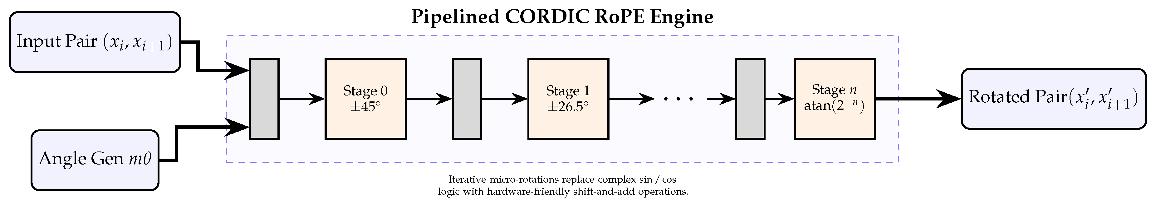
Implementing sine and cosine functions for every token in hardware is computationally expensive. Recent research highlights the Hummingbird architecture, which utilizes a CORDIC-based approximation for RoPE [6]. By leveraging the similarity between the rotary transformation and CORDIC rotations, the hardware can perform position embedding using only shift-and-add operations. This design saves up to in area cost compared to fixed-point implementations while maintaining negligible loss in model perplexity.
Figure 2.
Hardware implementation of Rotary Position Embeddings (RoPE) via CORDIC logic. The design uses a systolic pipeline of micro-rotation stages to approximate the rotation of token features based on their sequence position.
Figure 2.
Hardware implementation of Rotary Position Embeddings (RoPE) via CORDIC logic. The design uses a systolic pipeline of micro-rotation stages to approximate the rotation of token features based on their sequence position.
3.3. Output Decoders and De-Quantization
The "Output Decoder" (the final Linear + Softmax layer) faces a similar memory bottleneck. Efficient hardware like the FlashHead architecture [7] uses equal-sized spherical clustering to organize token embeddings. This enables predictable memory layouts and fast access patterns on both GPUs and edge-AI accelerators, allowing the output projection to run at a fraction of the traditional computational cost.
3.3.1. Hardware-Aware De-Quantization
In the last few years, many LLMs use Mixed-Precision Quantization (e.g., INT4 weights with FP16 activations). The input/output stages must therefore include specialized De-quantization Engines that perform on-the-fly rescaling of weights before they enter the systolic array. These engines are often fused with the memory controllers to ensure that the compute units never stall while waiting for high-precision conversion.
In this architecture, weights are stored in INT4 to save 75% of memory footprint compared to FP16 as it is shown in Figure 3. The De-quantization Engine performs a fused "Scale and Shift" operation to bring the weights back to the FP16 domain (or a microscaling format) just-in-time for the Matrix Multiply-Accumulate (MMA) operation.
Bandwidth Efficiency: By transferring INT4 weights, the hardware reduces the "Memory Wall" pressure by compared to FP16. ALso, to prevent the systolic array from idling, the de-quantization engine is typically a pipelined multiplier-adder unit. It applies the formula as weights are fetched from the memory controller.
4. Multi-Head Attention (MHA) Architecture
The Multi-Head Attention (MHA) mechanism is the computational core of the Transformer architecture, responsible for capturing dependencies across different positions in a sequence. From a hardware perspective, MHA is the most challenging component due to its high computational complexity ( with respect to sequence length n) and significant memory bandwidth requirements.
4.1. Mathematical Formulation
In MHA, the input sequence is projected into three distinct spaces: Queries (Q), Keys (K), and Values (V). Instead of performing a single attention function, the model runs multiple "heads" in parallel, allowing the system to attend to information from different representation subspaces simultaneously [2].
For each head i, the attention is calculated as:
The final output is a concatenation of all heads, multiplied by an output projection matrix :
4.2. Hardware Operational Flow
Implementing MHA in digital logic requires decomposing these matrix operations into a hardware-friendly dataflow. The operation can be broken down into four primary hardware stages:
- 1.
- Linear Projection: Input vectors are multiplied by weight matrices (). In hardware, this is implemented using Systolic Arrays or General Matrix Multiply (GEMM) engines optimized for the target precision (e.g., FP16, INT8, or Microscaling formats like MXFP8 [4]).
- 2.
- MatMul Score Calculation (): This stage computes the similarity scores. For long sequences, this creates a massive intermediate "Score Matrix." Hardware accelerators often use tiling strategies to keep these scores in on-chip SRAM to avoid costly DRAM access.
- 3.
- Softmax Normalization: This is a non-linear operation involving exponentiation and division. Digital implementation typically utilizes CORDIC algorithms or Taylor series expansions, often combined with a "Streaming Softmax" approach to reduce latency [8].
- 4.
- Weighted Sum (): The normalized scores are used to weight the Value vectors. This requires another GEMM operation, often pipelined directly after the Softmax unit.
Challenges in Digital Design: The primary bottleneck for MHA in RTL design is the quadratic growth of the attention matrix. As the sequence length n increases, the memory required to store exceeds the capacity of typical on-chip buffers. To mitigate this, modern hardware implementations leverage FlashAttention principles, which fuse the MatMul and Softmax operations into a single kernel to minimize off-chip memory traffic [3].
In the following section we present the most efficient hardware architectures for each component of the Mult-Head Attention.
4.3. Hardware Design of Linear Projections
Linear projections, also known as fully connected or dense layers, form the computational backbone of both the Multi-Head Attention (MHA) and the Feed-Forward Network (FFN). In the context of LLMs, these operations typically manifest as General Matrix Multiplications (GEMM) during the prefill (encoding) stage and General Matrix-Vector Multiplications (GEMV) during the decode (token generation) stage.
4.3.1. Architectural Implementation: Systolic Arrays
The most efficient hardware implementation for linear projections in modern accelerators is the Systolic Array. This architecture minimizes the need for high-bandwidth global memory access by reusing data across a 2D mesh of Processing Elements (PEs) [2].
Typical dataflow strategies include:
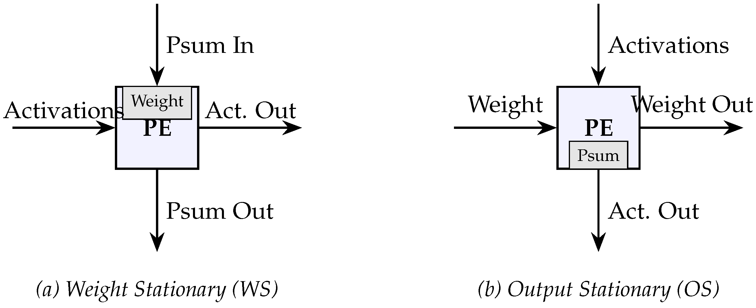
- Weight Stationary (WS): In a Weight Stationary architecture, each processing element (PE) pre-loads a weight value and stores it in its internal register for the duration of a compute cycle. Input activations are then streamed horizontally through the array, while partial sums (psums) are accumulated vertically. This is ideal for scenarios where the weight matrix is significantly larger than the activations. It is best for Transformer encoding (prefill) stages where the weight matrix is reused across many tokens. The main advantage is that it minimizes the energy-intensive process of fetching weights from the Global Buffer (GB) or DRAM.
- Output Stationary (OS): In an Output Stationary architecture, the weight and activation data move through the array, but the partial sums remain fixed in the PE’s accumulator until the final output value is fully computed. Since partial sums remain in the PEs until the final output is computed, this leads to reduced traffic associated with writing intermediate results back to the scratchpad memory. This option is best for transformer decoding (token generation) or scenarios with small batch sizes where minimizing the write-back of intermediate partial sums is critical. The main advantage is that it reduces the traffic on the accumulation bus and the number of scratchpad memory writes.
Figure 4.
Processing Element (PE) Dataflows for Matrix Multiplication.
The state-of-the-art in linear projection hardware has shifted toward domain-specific numerical formats and asynchronous data movement to combat the "Memory Wall."
4.3.2. Low-Precision and Microscaling Formats
As of 2026, the industry has widely adopted Microscaling (MX) formats. Unlike traditional floating-point formats where every number has its own exponent, MX formats (like MXFP8 and MXINT4) group vectors of elements to share a single scaling factor. This reduces the hardware area of the multiplier-accumulator (MAC) units by up to 40% while maintaining model accuracy [4].
4.3.3. NVIDIA Blackwell (B200) Architecture
The fifth-generation Tensor Cores in the NVIDIA Blackwell B200 represent the current gold standard for linear projection hardware. Key innovations include:
- Native FP4 Support: The introduction of 4-bit floating point (FP4) doubles the throughput of linear projections compared to FP8, reaching up to 20 PetaFLOPS of AI performance per GPU [9].
- Second-Generation Transformer Engine: This logic dynamically manages precision at a per-layer or per-tensor level, ensuring that the linear projection units operate at the lowest possible precision without diverging.
- Tensor Memory (TMEM): A dedicated memory pathway that allows Tensor Cores to fetch operands directly from shared memory without warp-level synchronization, reducing idle cycles in the pipeline [10].
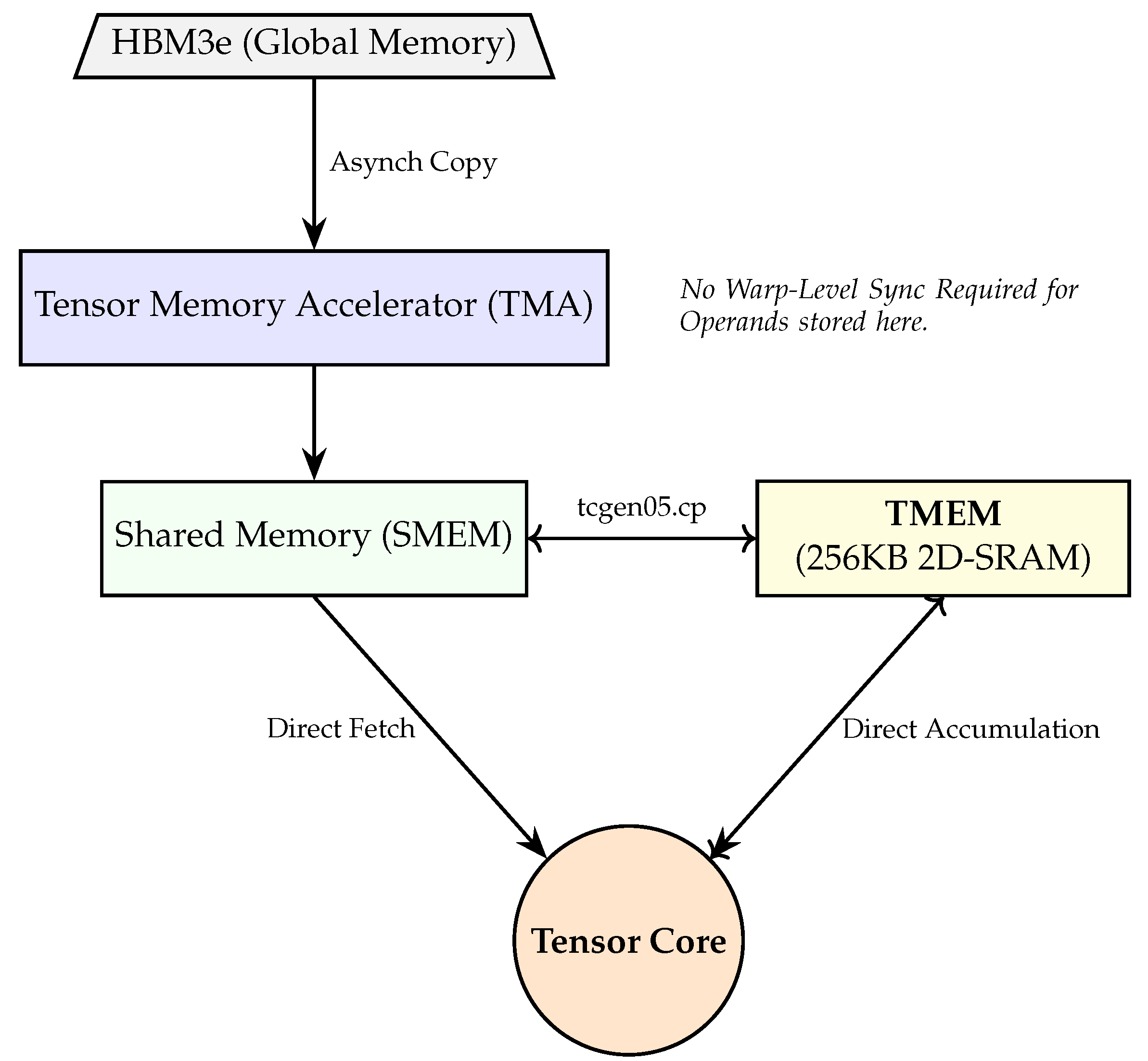
A major architectural shift in the last years is the introduction of Tensor Memory (TMEM) (i.e. NVIDIA Blackwell architecture). This dedicated 256,KB memory structure within the Streaming Multiprocessor (SM) acts as a high-bandwidth staging area for the fifth-generation Tensor Cores, fundamentally altering how data is fetched and synchronized during matrix operations.
In previous architectures (e.g., Ampere and Hopper), matrix multiply-accumulate (MMA) operations were strictly warp-synchronous. This required all 32 threads in a warp to synchronize and participate in the instruction simultaneously, creating idle "barrier" cycles.
Blackwell’s TMEM enables a warp-level independent scheduling model. Through the new tcgen05.mma instruction, the hardware can fetch operands directly from Shared Memory (SMEM) or TMEM without requiring warp-wide synchronization. This "Single-Thread/Single-Warp" dispatch allows for better instruction-level parallelism (ILP) and masks the latency of data movement [11,12].
The following TikZ diagram illustrates the dual pathways: the asynchronous loading via the Tensor Memory Accelerator (TMA) and the direct, synchronization-free pathway between TMEM and the Tensor Cores.
By utilizing TMEM as a 2D-organized scratchpad (512 columns × 128 lanes), the hardware achieves:
- Reduced Register Pressure: Large accumulators reside in TMEM rather than the Register File (RF), freeing up RF space for other complex operations like LayerNorm or RoPE [13].
- Higher Bandwidth: TMEM provides an effective bandwidth of ∼100,TB/s within the SM, which is 2.5× the speed of the aggregate L1/Shared Memory pathway.
- Synchronization Latency Hiding: Because operands are fetched directly from TMEM, the pipeline does not stall for warp-level coordination, reducing the time-to-first-token (TTFT) by up to for long-context sequences [12].
Figure 5.
The Blackwell TMEM hierarchy. TMA asynchronously stages data into SMEM, while TMEM provides a dedicated pathway to Tensor Cores, bypassing register file pressure and warp-synchronization overhead.
Figure 5.
The Blackwell TMEM hierarchy. TMA asynchronously stages data into SMEM, while TMEM provides a dedicated pathway to Tensor Cores, bypassing register file pressure and warp-synchronization overhead.
| TMEM |
| (256KB 2D-SRAM) |
4.3.4. Processing-in-Memory (PIM)
Finally, for edge-based LLM implementations, recent research focuses on PIM-based linear layers. By integrating MAC units directly into the peripheral circuitry of HBM or SRAM, systems like Pyramid [14] eliminate the energy cost of moving weights across the data bus, which is the primary bottleneck during the memory-bound GEMV operations of the decoding stage.
4.4. Attention Score Calculation MatMul:
The computation of the attention score matrix, denoted as , represents the most critical bottleneck in Transformer hardware design for long-sequence tasks. Unlike the linear projections, this operation exhibits quadratic complexity relative to sequence length n, necessitating specialized dataflow management to handle the resulting memory and compute explosion.
To implement this in digital logic efficiently, the design must move away from materializing the full score matrix in global memory (High Bandwidth Memory: HBM). Modern hardware-friendly algorithms focus on:
- Single-Pass Pipelining: For decoding stages where the input is a single query vector, algorithms like SwiftKV Attention enable a per-token pipelined architecture. This allows the hardware to process KV cache entries exactly once without storing intermediate scores, significantly reducing latency on edge accelerators [16].
- Block-Sparse Approximations: Recent implementations such as SALE utilize low-bit quantized query-key products to estimate the importance of token pairs. Only the "sink" and "local" regions of the attention map—which contain the highest scores—are computed at high precision, enabling a speedup for 64K context windows [17].
Efficient Hardware Realizations: State-of-the-art (SOTA) hardware for score calculation as of 2026 leverages custom data movement engines and specialized arithmetic units:
4.4.1. NVIDIA Blackwell (B200) Tensor Memory
As it was described above in the case on Linear Projectsion, the Blackwell architecture introduces the Tensor Memory Accelerator (TMA) and Tensor Memory (TMEM), which are pivotal for operations. TMA allows for asynchronous data transfers between HBM and shared memory, overlapping the heavy key-matrix loading with query computation. TMEM provides a dedicated 256KB scratchpad per SM, allowing the scores to be stored and normalized locally before the final value-multiplication stage [11].
4.4.2. SwiftKV-MHA Accelerator
For edge and computer engineering applications, the SwiftKV-MHA architecture represents the most efficient specialized design. It utilizes a unified processor array that supports high-precision attention scores alongside low-precision GEMV operations. By integrating a "Streaming Softmax" unit directly into the MatMul pipeline, it achieves a reduction in attention latency compared to general-purpose implementations [16].
4.4.3. WGMMA Instructions
Modern hardware utilizes Warpgroup Matrix Multiply-Accumulate (WGMMA) instructions. These allow groups of 128 threads to coordinate a single large matrix operation, effectively treating the individual Processing Elements (PEs) as a single high-throughput engine for the Query-Key dot products. This minimizes register pressure, which is often the limiting factor when managing large attention heads [11].
4.5. FPGAs
Contemporary FPGAs have infused novel AI blocks that are used to improve the performance of Multi-Head Attention algoriths. For example, Altera Agilex 5 and Agilex 3 FPGAs have fabric infused with AI Tensor Blocks, giving higher compute density per DSP block of 20 block floating point 16 (Block FP16) or int8 multiply accumulate (MAC) blocks. Other lower precisions, such as FP9 and INT4, are supported in the DSP blocks, which greatly helps accelerate the performance and latency of the most used functions in the LLM models and reduce the model sizes, improving computational efficiencies and memory footprint as it is shown in Figure 6.
4.6. Softmax Normalization in Hardware
The Softmax unit is a critical non-linear component that normalizes the attention scores. It transforms a vector of attention scores into a probability distribution, ensuring that all values range between (0, 1) and sum to unity.
For an input vector x of length n, the Softmax output for element is defined as:
Figure 7 shows how Softmax compares to a simple identity or sigmoid. It highlights the "winner-take-all" nature when one value is significantly higher than others.
Figure 8 illustrates the typical "three-pass" hardware nature: Exponential calculation, Summation, and final Division.
Table 3.
Hardware implementations of SoftMax.
| Implementation | Complexity | Latency | Efficiency |
|---|---|---|---|
| Exaxt | High | High | Low |
| CORDIC | Low | High | Medium |
| LUT | Medium | Low | High |
- Pass 1: Exponential Calculation: Input logits are processed through Non-Linear Units (NLUs)—typically utilizing Look-Up Tables (LUTs), CORDIC, or piecewise linear approximations—to compute . To prevent numerical overflow, hardware designs often subtract the maximum logit () before exponentiation.
- Pass 2: Summation: The exponential results are streamed into a high-precision accumulator to calculate the global denominator, . This pass acts as a synchronization barrier, as the final probability cannot be determined until the sum of the entire vector is finalized.
- Pass 3: Normalization/Division: Each stored or recomputed exponential value is normalized by the global sum. In digital logic, this is often implemented as a multiplication by the reciprocal () to improve throughput, as hardware dividers are significantly more area-intensive than multipliers.
In digital design, the Softmax operation is particularly challenging due to the exponential function , which requires significant hardware resources and is prone to numerical overflow. Modern hardware accelerators for 2026 employ several approximation strategies to balance resource utilization, latency, and numerical precision.
4.6.1. Approximation Strategies for the Exponential Function
Direct implementation of the transcendental exponential function is avoided in high-speed hardware implementations. Instead, four primary hardware-centric methods are utilized, each one with advantages and disadvantages:
- CORDIC-based Implementation: The COordinate Rotation Digital Computer (CORDIC) algorithm is a versatile iterative method that computes hyperbolic and transcendental functions using only shifts and additions. To compute , CORDIC operates in the hyperbolic vectoring mode. By decomposing the exponent into a series of predefined elementary rotation angles, the hardware performs a sequence of iterative micro-rotations. CORDIC is highly area-efficient as it eliminates the need for multipliers or large memory blocks (BRAM/SRAM). However, it introduces significant latency due to its iterative nature (typically n cycles for n-bit precision) [18].
- LUT-based Exponential Units: As of 2026, Look-Up Table (LUT) approaches are the preferred standard for high-throughput LLM accelerators like the NVIDIA Blackwell (B200) and specialized FPGAs.
- Bipartite LUTs: To further reduce memory footprint, bipartite LUTs use two smaller tables to store the most significant and least significant parts of the approximation, which are then combined via a single addition [19].
- Piecewise Linear Approximation (PLA): The exponential curve is divided into segments, and each segment is approximated by a linear equation . The coefficients a and b are stored in a small LUT.
In digital hardware, the direct implementation of this equation is prone to numerical overflow due to the exponential function. Additionally, the three-pass structure imposes a significant latency penalty and increases memory traffic, as intermediate values must often be buffered in SRAM. To mitigate this, hardware designs utilize the SafeSoftmax algorithm, which subtracts the maximum value from each element before exponentiation:
This ensures that all exponents are non-positive (), constraining the output of to the range and preventing bit-overflow in fixed-point or floating-point registers [20].
Modern hardware accelerators have moved away from standard library functions toward specialized non-linear arithmetic units (NLUs) that prioritize throughput and area efficiency.
4.6.2. Log-Domain Division and Bipartite LUTs
One of the most efficient implementations for edge and FPGA-based accelerators involves transforming the division operation into a subtraction in the logarithmic domain. Instead of using a resource-intensive hardware divider, recent designs like SOLE [21] utilize a bipartite Look-Up Table (LUT) to approximate the exponential and logarithmic functions. By representing the sum in the log-domain, the hardware can perform the final normalization using simple subtraction units and bit-shifters, achieving up to a improvement in area efficiency over traditional designs.
4.6.3. Streaming (Online) Softmax
To reduce the memory bottleneck of the "three-pass" Softmax (Max → Sum → Divide), modern GPUs and ASICs implement Online Softmax. This algorithm computes the running maximum and the partial sum-of-exponentials in a single pass over the data. In architectures like NVIDIA’s Blackwell (B200), this is further optimized into the FlashAttention-4 kernel, where the Softmax rescaling is fused directly with the Matrix-Multiply-Accumulate (MMA) pipeline, eliminating the need to write intermediate scores to HBM [22].
4.6.4. Skip Softmax and Sparsity
As of late 2025, the Skip Softmax algorithm has been integrated into SOTA hardware like the NVIDIA GB200. This implementation exploits the observation that if is a large negative number, . The hardware logic dynamically identifies these "negligible" blocks and skips the exponential and subsequent multiplication operations entirely, delivering up to a speedup in time-to-first-token (TTFT) for long-context windows [23].
4.6.5. Base-2 Transformation:
Hardware-friendly "Softermax" implementations often transform into . Since can be implemented in digital logic using a simple bit-shift (for integer parts) and a small LUT (for fractional parts), this method significantly reduces the "Energy Wall" [24].
4.6.6. Fusion with Attention:
SOTA kernels like FlashAttention-4 (2026) move the Softmax unit directly into the Tensor Core pipeline. By using software-emulated exponentials (FMA-based polynomial approximations), the hardware can overlap the Softmax normalization with the next Matrix Multiply-Accumulate (MMA) operation, achieving up to hardware utilization on the Blackwell architecture [22].
4.6.7. The E2Softmax Architecture
The E2Softmax (Efficient log2 quantized Softmax) unit, integrated within the SOLE framework is based on Log-Domain Subtraction; Rather than performing a traditional division (), E2Softmax performs subtraction in the log-domain. The hardware identifies the maximum logit m, computes , and uses a multiplier-free shift-add pipeline to generate normalized probabilities. Recent ASIC implementations at the 28nm node demonstrate a speedup and over energy efficiency gains compared to conventional 16-bit LUT approaches, with an accuracy loss of less than [25].
5. Feed-Forward Network (FFN) Hardware Design
In modern Transformer architectures, the Feed-Forward Network (FFN) accounts for approximately two-thirds of the total parameter count. While Multi-Head Attention (MHA) manages spatial dependencies across tokens, the FFN operates as a position-wise nonlinear transformation, effectively serving as the "knowledge store" of the model.
5.1. Architectural Shift: From ReLU to SwiGLU
Earlier models like GPT-2 and BERT utilized standard FFNs with ReLU or GeLU activations.
The Rectified Linear Unit (ReLU) is the most computationally efficient activation function in digital design. Unlike Softmax or SwiGLU, which require transcendental functions or multipliers, the ReLU operation is defined as:
.
In hardware, specifically when using Two’s Complement representation, the ReLU operation is implemented using the Most Significant Bit (MSB), which serves as the sign bit. If the sign bit is 0, the number is positive; if it is 1, the number is negative.The most efficient hardware implementation utilizes a 2-to-1 Multiplexer (MUX) where the select signal is the inverted sign bit of the input (Figure 9.
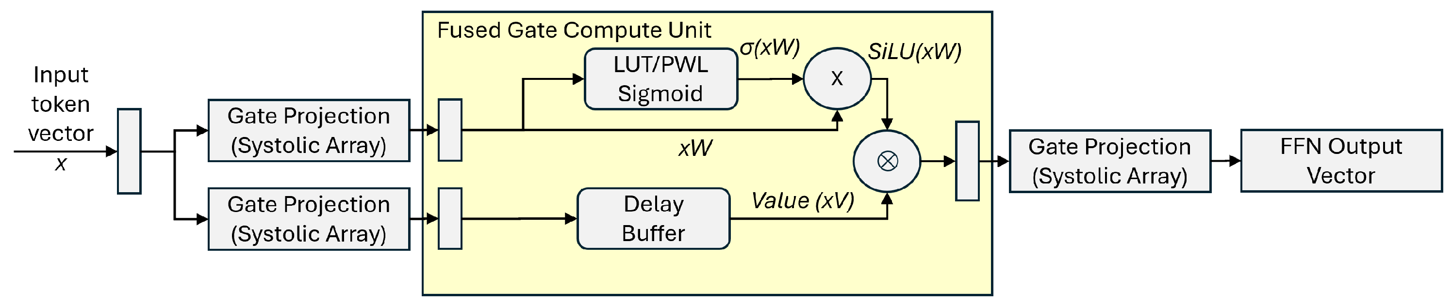
However, state-of-the-art models in 2026 (e.g., Llama 4, Qwen 3, and DeepSeek-V3) have shifted to the SwiGLU (Swish-Gated Linear Unit) architecture. This design replaces the two-layer MLP with a three-matrix gated structure, offering superior convergence and expressivity [26]. The SwiGLU operation for an input x is defined as:
where W and V are the gate and primary projection matrices, is the down-projection matrix, and ⊗ denotes element-wise (Hadamard) multiplication.
From a digital design perspective, SwiGLU introduces a "dual-stream" dataflow. This requires parallelized execution units that can handle two simultaneous matrix-vector multiplications followed by a fused nonlinear activation and Hadamard product.
5.1.1. Gated Pipeline Architecture
The most efficient hardware realization utilizes a Fused-Gate-Compute unit. Instead of storing the intermediate results of and in global memory, modern accelerators like the Flash-FFN engine (2025) compute both projections in parallel within the same systolic array pass [27].
- Parallel Projection: A bifurcated systolic array or a "Wide-MAC" unit processes W and V concurrently.
- SiLU Activation: The SiLU (Sigmoid Linear Unit) function () is implemented using a high-speed piecewise linear (PWL) approximation or a small LUT-based sigmoid generator.
- On-the-fly Hadamard: The multiplication of and is performed in the local register file to minimize toggle activity and power consumption.
Figure 11 shows the input vector x splitting immediately into two parallel paths. Top Path (Gate Stream) flows through the W projection systolic array while Bottom Path (Value Stream) flows through the V projection systolic array.
The prompt specified is implemented via LUTs/PWL. The diagram details this by showing the top stream splitting again:One sub-path goes into the "LUT/PWL Sigmoid " block. The other sub-path bypasses it. They recombine at a standard multiplier (×) to form the SiLU output. In real hardware, the SiLU operation takes several clock cycles. The diagram includes a "Latency Matching FIFO/Delay Buffer" on the bottom (Value) stream to ensure that arrives at the Hadamard multiplier at the exact same clock cycle as .
The central orange circle represents the element-wise multiplication where the "gating" actually occurs, combining the two streams. The dashed background box visually groups the activation, delay, and Hadamard operations, indicating to the reader that these operations are likely fused into a tightly coupled pipeline stage operating on local registers, rather than writing intermediate results back to global memory.
The Hadamard product (or element-wise multiplication) is used to gate information streams. Unlike a standard Matrix Multiplication (GEMM), which involves an accumulation of products across an entire row/column, the Hadamard product of two tensors A and B of the same dimension is defined simply as:
From a digital design perspective, the Hadamard multiplier is significantly less complex than a systolic array. Since there is no cross-element dependency or accumulation tree required, the hardware implementation consists of a parallel array of independent Multiplier units (n units for a vector of size n).Key hardware characteristics include:
- Parallel Datapaths: and are fed into the i-th multiplier simultaneously.
- High Throughput: Because there are no partial sum reductions, the operation is perfectly parallelizable and can be fully pipelined with a latency of only a few clock cycles (depending on the precision, e.g., FP16 or INT8).
- Memory Alignment: The primary bottleneck is ensuring that both operands A and B arrive at the execution units at the same time. This often requires synchronized FIFO buffers or dual-port SRAM blocks to handle the dual-stream data fetch.
The following diagram illustrates a hardware architecture for an n-wide Hadamard multiplier unit, typical for a vector processor or an LLM accelerator’s FFN gating stage.
Figure 10.
Hardware block diagram of a parallel Hadamard Multiplier. This unit enables the "gating" mechanism in SwiGLU by performing simultaneous multiplication across all vector lanes.
Figure 10.
Hardware block diagram of a parallel Hadamard Multiplier. This unit enables the "gating" mechanism in SwiGLU by performing simultaneous multiplication across all vector lanes.
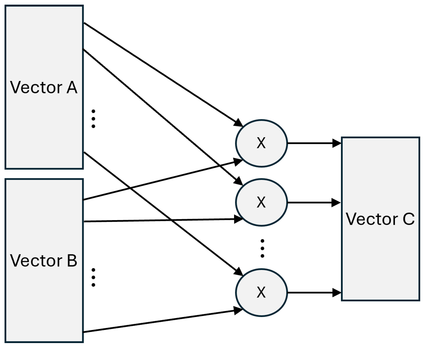
Figure 11.
Hardware Block Diagram of the SwiGLU FFN architecture. It illustrates the "dual-stream" dataflow where the Gate (W) and Value (V) projections occur in parallel. The Gate stream is processed by a hardware SiLU unit (comprising a LUT-based sigmoid and a multiplier) before gating the Value stream via an element-wise Hadamard product (⊗).
5.2. State-of-the-Art: LUT-LLM and Memory-Based Computation
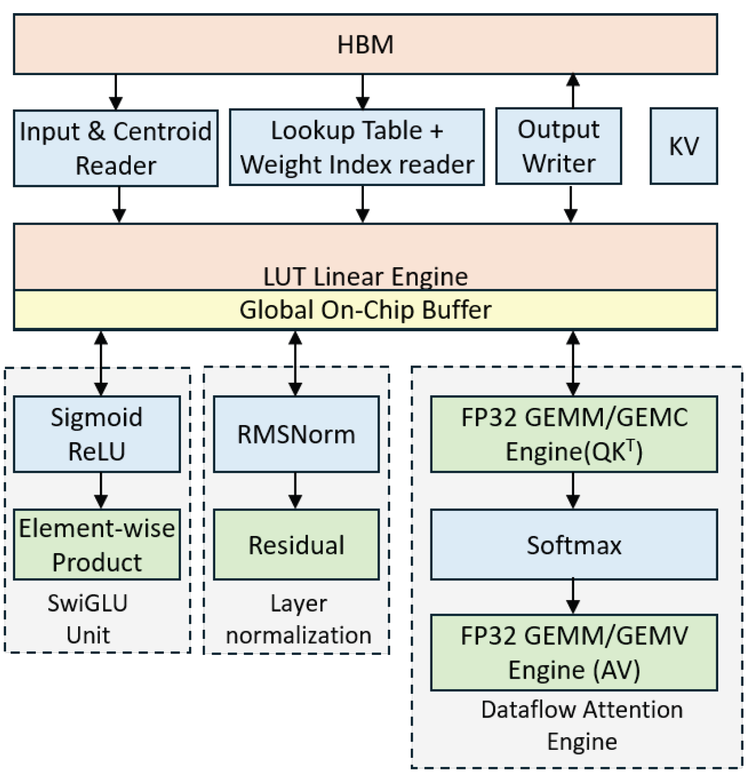
The most recent leap in FFN hardware efficiency is LUT-LLM. This architecture replaces traditional multipliers in the FFN with specialized memory-based lookup tables for the nonlinear stages.LUT-LLM employs a spatial-temporal hybrid design, integrating a sequential LUTLinear engine with a dataflow attention engine, which optimizes on-chip memory management and throughput for both prefill and decode stages. By mapping the SiLU-Gating operation into high-density SRAM macros, LUT-LLM achieves a higher energy efficiency than the NVIDIA A100 for FFN-heavy workloads [28]. LUT-LLM features a bandwidth-aware parallel centroid search, co-designed with memory bandwidth, to significantly reduce decoding latency and maximize compute engine throughput as it is shown in Figure 12.
6. Conclusion and Future Outlook
The rapid evolution of Large Language Models (LLMs) and Multimodal Models (LMMs) has fundamentally shifted the requirements for digital hardware design. As this tutorial has demonstrated, the transition from general-purpose computing to domain-specific architectures is no longer optional; it is a necessity driven by the physical limits of power density and memory bandwidth. Efficient hardware implementations of the Transformer backbone—specifically optimized Multi-Head Attention, pipelined SwiGLU FFNs, and fused de-quantization engines—are the only path toward sustainable and real-time AI.
6.1. The Necessity of Hardware-Software Co-Design
The performance gains of the 2025–2026 era, such as those seen in the NVIDIA Blackwell and specialized LUT-LLM architectures, stem from a tight coupling of algorithmic breakthroughs (like FlashAttention) and low-level RTL optimizations. Digital designers must continue to move away from monolithic compute units toward distributed, memory-centric architectures where the "cost" of a clock cycle is measured not in FLOPs, but in Joules-per-byte moved.
6.2. Emerging Technologies and Radical Architectures
Looking beyond 2026, several emerging technologies promise to break the remaining bottlenecks of the Transformer architecture:
- Neuromorphic and Event-Based Computing: By leveraging spiking neural networks (SNNs), future accelerators may achieve extreme sparsity. Neuromorphic hardware only "fires" when significant information is detected, potentially reducing the energy consumption of the FFN layers by orders of magnitude.
- Optical and Photonic Interconnects: To solve the "Memory Wall," research into silicon photonics aims to replace electrical copper traces with light-based data movement, enabling Terabit-per-second bandwidth between HBM and the compute core with near-zero heat dissipation.
- Analog In-Memory Computing (AiMC): While this tutorial focused on digital logic, analog crossbar arrays (using ReRAM or Phase-Change Memory) are emerging as a way to perform matrix multiplications at the location of the data itself, bypassing the Von Neumann bottleneck entirely.
- Sub-2-bit and 1-bit Quantization: As quantization theory reaches the "Binary/Ternary" limit, hardware will transition from complex floating-point units to simple bit-manipulation logic, allowing for massive parallelization on a single die.
In summary, the future of LLM hardware lies in the "death of the general-purpose chip." The next decade of computer engineering will be defined by silicon that is as adaptive and specialized as the neural architectures it seeks to run.
References
- Varghese, G.; Xu, J. Network Algorithmics: An Interdisciplinary Approach to Designing Fast Networked Devices, 2nd ed.; Morgan Kaufmann, 2022. [Google Scholar] [CrossRef]
- Vaswani, A.; Shazeer, N.; Parmar, N.; Uszkoreit, J.; Jones, L.; Gomez, A.N.; Kaiser; Polosukhin, I. Attention is all you need. In Proceedings of the Advances in neural information processing systems, 2017; pp. 5998–6008. [Google Scholar]
- Dao, T.; Fu, D.Y.; Ermon, S.; Rudra, A.; Ré, C. Flashattention: Fast and memory-efficient exact attention with io-awareness. arXiv arXiv:2205.14135.
- OCP Microscaling Formats (MX) Specification v1.0. Open Compute Project Technical report. 2024.
- Lee, J. Near-Memory Processing in Action: Accelerating Personalized Recommendation With AxDIMM. IEEE Micro; 2025. [Google Scholar]
- Contributors, R. Efficient Hardware Architecture Design for Rotary Position Embedding of Large Language Models. arXiv 2026. arXiv:2601.39036.
- Engineering, E. Ultra-Efficient SLMs: Embedl’s Breakthrough for On-Device AI. Technical Whitepaper, 2025. [Google Scholar]
- Rabe, M.N.; Staats, C. Self-attention Does Not Need O(n2) Memory. arXiv arXiv:2112.05682.
- Team, C.E. NVIDIA B200 GPU Guide: Use Cases, Models, and Benchmarks. Clarifai Technical Blog 2026. [Google Scholar]
- Jarmusch, A.; Chandrasekaran, S. Microbenchmarking NVIDIA’s Blackwell Architecture: An in-depth Architectural Analysis. arXiv arXiv:2512.02189.
- Team, M. Matrix Multiplication on Blackwell: Part 1 - Introduction. Modular Technical Blog, 2025. [Google Scholar]
- Research, E.M. Blackwell GPU Architecture: Microbenchmarking and Performance Analysis. arXiv 2026. arXiv:2601.10953.
- Vishnumurthy, N. NVIDIA Blackwell Architecture: A Deep Dive into the Next Generation of AI Computing. Medium Technical Publication, 2025. [Google Scholar]
- Lee, J. Pyramid: Accelerating LLM Inference With Cross-Level Processing-in-Memory. In Proceedings of the IEEE Computer Architecture Letters, 2025. [Google Scholar]
- Engineering, N. Overcoming Compute and Memory Bottlenecks with FlashAttention4 on NVIDIA Blackwell. NVIDIA Technical Blog, 2026. [Google Scholar]
- Zhang, Junming; Zhang, Qinyan; H.S.F.G.S.H.R.N.X.M. SwiftKV: An Edge-Oriented Attention Algorithm and Multi-Head Accelerator for Fast, Efficient LLM Decoding. arXiv 2026. arXiv:2601.10953.
- Review, U. SALE: Low-Bit Estimation for Efficient Sparse Attention in Long-Context LLM Prefilling. In Proceedings of the ICLR 2026 Conference Submission, 2026. [Google Scholar]
- Vatalaro, M. Comparative Study on CORDIC Accelerators for NCO and Nonlinear Applications. In Lund University Publications; 2025. [Google Scholar]
- Wang, W.; Zhou, S. SOLE: Hardware-Software Co-design of Softmax and LayerNorm for Efficient Transformer Inference. In Proceedings of the ICCAD 2025, 2025. [Google Scholar]
- Li, W.J. Hardware-oriented algorithms for softmax and layer normalization of large language models. Science China Information Sciences 2024, 67. [Google Scholar] [CrossRef]
- Wang, W.; Zhou, S.; Sun, W.; Liu, Y. SOLE: Hardware-Software Co-design of Softmax and LayerNorm for Efficient Transformer Inference. arXiv arXiv:2510.17189.
- Engineering, D. FlashAttention 4: Faster, Memory-Efficient Attention for LLMs. Practitioner Deep Dives, 2026. [Google Scholar]
- Blog, N.D. Accelerating Long-Context Inference with Skip Softmax in NVIDIA TensorRT-LLM. 2025. [Google Scholar]
- Stevens, J.R. Softermax: Hardware-Friendly Softmax Approximation for Transformers. arXiv 2024. arXiv:2401.12345.
- Research, E.M. E2Softmax: Efficient Hardware Softmax Approximation via Log-Domain Division. Technical Report. 2026. [Google Scholar]
- Shojaei, M. SwiGLU: The FFN Upgrade for State of the Art Transformers. DEV Community, 2025. [Google Scholar]
- Chen, H. Flash-FFN: A Pipelined Accelerator for Gated Linear Units. In Proceedings of the Symposium on High-Performance Computer Architecture (HPCA), 2025. [Google Scholar]
- Review, U. LUT-LLM: Efficient Large Language Model Inference with Memory-based Computations on FPGAs. arXiv arXiv:2511.06174.
Figure 1.
Comparison of Data Movement for Embedding Lookups. (a) Traditional systems move large amounts of raw data to the compute unit. (b) Near-Memory Processing (AxDIMM). Logic units integrated into the DIMM perform embedding lookups locally, transmitting only minimal data.
Figure 1.
Comparison of Data Movement for Embedding Lookups. (a) Traditional systems move large amounts of raw data to the compute unit. (b) Near-Memory Processing (AxDIMM). Logic units integrated into the DIMM perform embedding lookups locally, transmitting only minimal data.
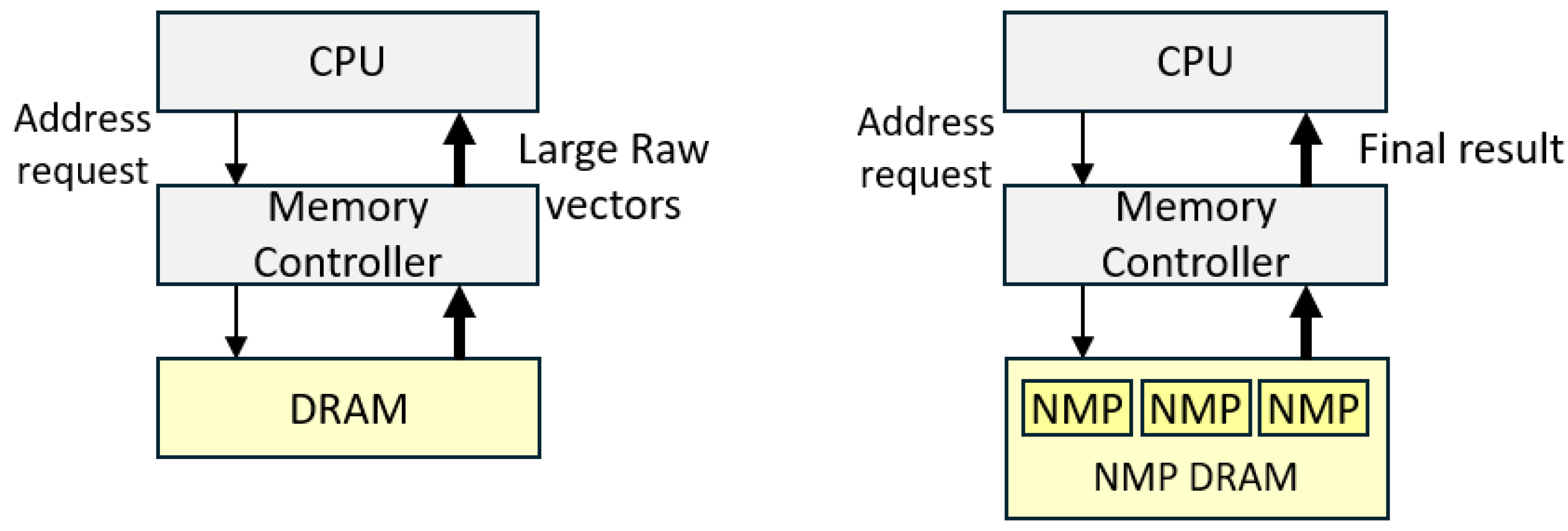
Figure 3.
Hardware dataflow for Mixed-Precision Quantization. Weights are stored and transferred in 4-bit (INT4) to save bandwidth, then rescaled to 16-bit (FP16) by a specialized de-quantization engine before being paired with high-precision activations in the systolic array.
Figure 3.
Hardware dataflow for Mixed-Precision Quantization. Weights are stored and transferred in 4-bit (INT4) to save bandwidth, then rescaled to 16-bit (FP16) by a specialized de-quantization engine before being paired with high-precision activations in the systolic array.
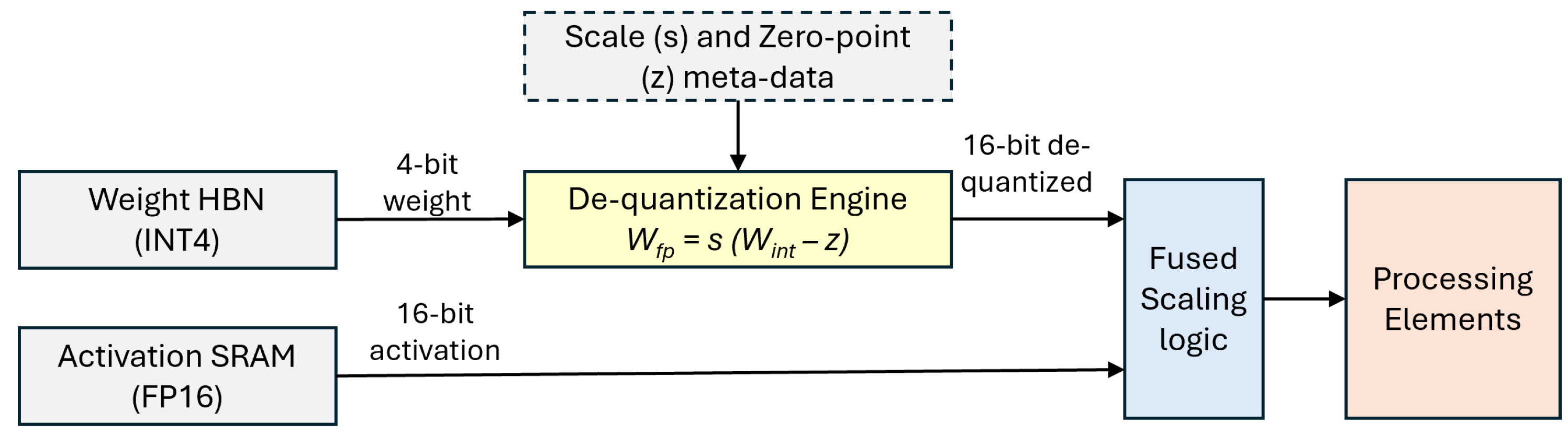
Figure 6.
Agilex 5 FPGA infused with with AI modules of 20 block floating point 16 (Block FP16) or int8 multiply accumulate (MAC) blocks.
Figure 6.
Agilex 5 FPGA infused with with AI modules of 20 block floating point 16 (Block FP16) or int8 multiply accumulate (MAC) blocks.
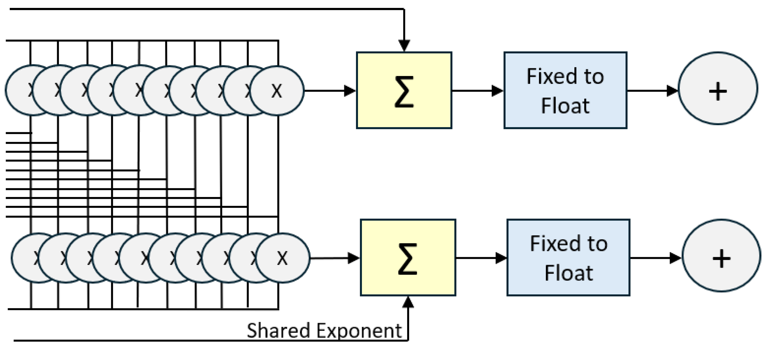
Figure 7.
Visualization of the Softmax function for two classes. Note how it smooths the transition into a probability in the range .
Figure 7.
Visualization of the Softmax function for two classes. Note how it smooths the transition into a probability in the range .
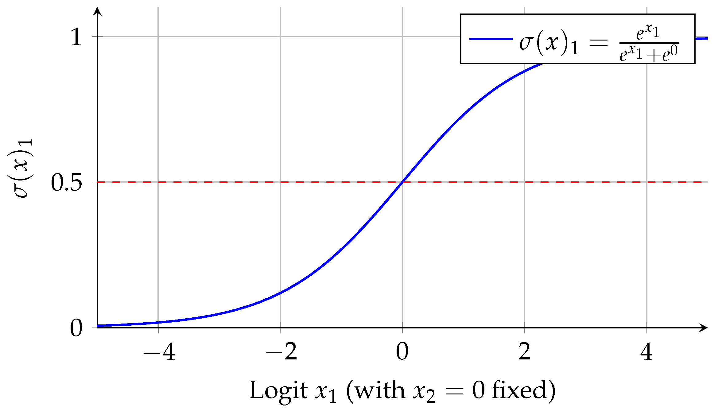
Figure 8.
Hardware Pipeline for Softmax Normalization. The scores are exponentiated, summed, and then the reciprocals are multiplied back to each element.
Figure 8.
Hardware Pipeline for Softmax Normalization. The scores are exponentiated, summed, and then the reciprocals are multiplied back to each element.
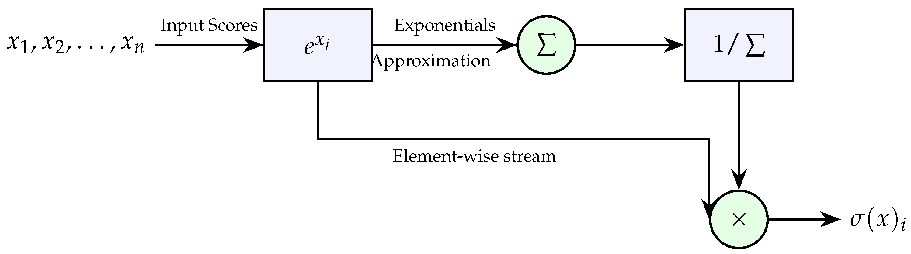
Figure 9.
The Rectified Linear Unit (ReLU) Activation. (a) The mathematical function showing non-linearity at zero. (b) ReLU Hardware Logic. In Two’s Complement, if the MSB is 1, the MUX selects the zero constant; otherwise, it passes the original input x.
Figure 9.
The Rectified Linear Unit (ReLU) Activation. (a) The mathematical function showing non-linearity at zero. (b) ReLU Hardware Logic. In Two’s Complement, if the MSB is 1, the MUX selects the zero constant; otherwise, it passes the original input x.
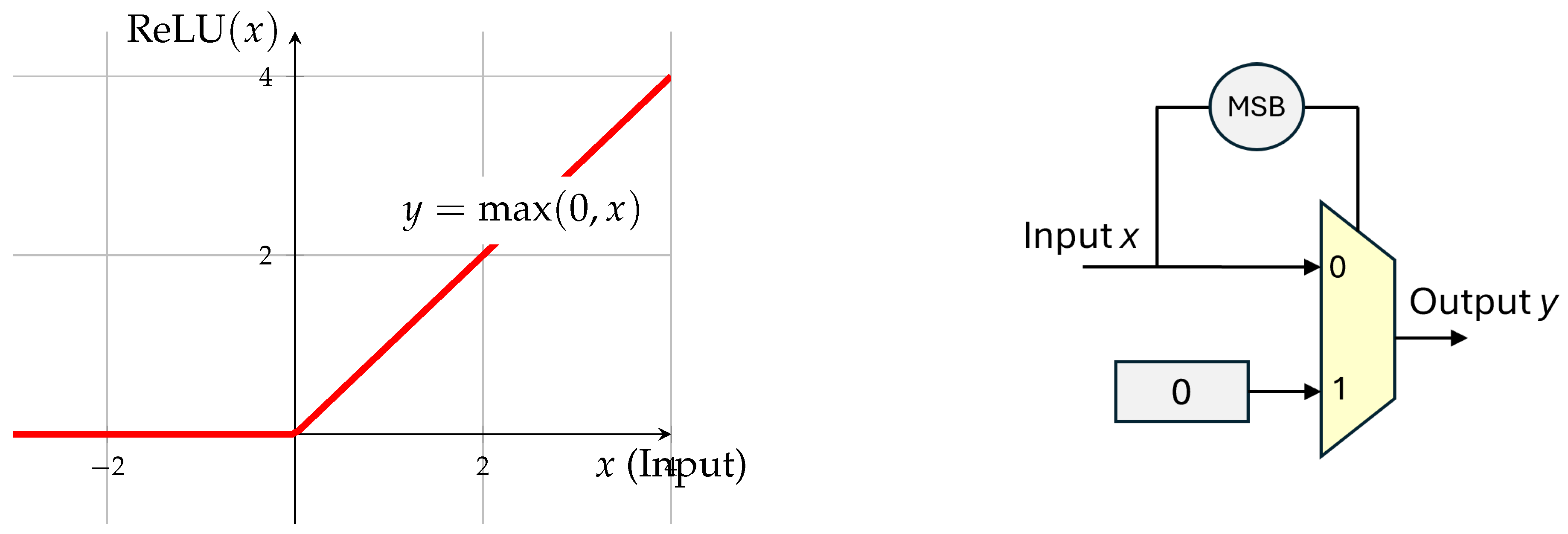
Figure 12.
The overall architecture of LUT-LLM, including a LUTLinear engine with global buffer, a dataflow attention engine, and special functions (SwiGLU, LayerNorm) with pipelined operations.
Figure 12.
The overall architecture of LUT-LLM, including a LUTLinear engine with global buffer, a dataflow attention engine, and special functions (SwiGLU, LayerNorm) with pipelined operations.
Disclaimer/Publisher’s Note: The statements, opinions and data contained in all publications are solely those of the individual author(s) and contributor(s) and not of MDPI and/or the editor(s). MDPI and/or the editor(s) disclaim responsibility for any injury to people or property resulting from any ideas, methods, instructions or products referred to in the content. |
© 2026 by the authors. Licensee MDPI, Basel, Switzerland. This article is an open access article distributed under the terms and conditions of the Creative Commons Attribution (CC BY) license (http://creativecommons.org/licenses/by/4.0/).
Copyright: This open access article is published under a Creative Commons CC BY 4.0 license, which permit the free download, distribution, and reuse, provided that the author and preprint are cited in any reuse.


