
Submitted:
05 February 2026
Posted:
09 February 2026
You are already at the latest version
Abstract
The European Union Emissions Trading System (EU ETS) has experienced dramatic price fluctuations since its 2005 inception, raising questions about whether carbon pricing effectiveness exhibits threshold behaviour—specifically, whether there exists a minimum carbon price level below which market signals fail to stimulate renewable energy investment. This study applies the Hansen threshold regression methodology to investigate regime-dependent dynamics in the relationship between EU ETS carbon prices and renewable energy consumption over 2005–2024. We identify a statistically significant threshold at €20.71/tCO2 (bootstrap p = 0.048), which partitions the sample into distinct low- and high-price regimes. Below this threshold, carbon prices exhibit no significant positive effect on renewable deployment (β1 = −36.16, p = 0.246); above the threshold, a positive relationship emerges (β2 = +7.20, p = 0.081), with each additional euro associated with 7.20 TWh of additional renewable consumption. Technol-ogy-specific analysis reveals that solar electricity exhibits particularly strong respon-siveness to above-threshold carbon prices (β2 = +1.71, p = 0.019). The threshold estimate is robust to alternative trimming specifications, functional forms, and outlier exclusion. These findings suggest that the EU ETS achieved effectiveness as a driver of renewable energy only after carbon prices exceeded approximately €21/tCO2—a transformation that coincided with the implementation of the Market Stability Reserve. The results provide empirical support for carbon price floor mechanisms and validate structural reforms aimed at strengthening the credibility of the carbon market.
Keywords:
EU ETS
; carbon pricing
; renewable energy
; threshold regression
; market stability reserve
; climate policy
; Hansen methodology
1. Introduction
The European Union Emissions Trading System (EU ETS), established in 2005 as the world’s first major carbon market, represents a cornerstone of European climate policy [1,2]. By pricing carbon dioxide emissions from power generation and industrial installations, the system aims to incentivise emissions reductions and stimulate investment in low-carbon technologies, including renewable energy sources [3,4]. Yet two decades of operational experience have revealed that carbon pricing effectiveness is neither linear nor guaranteed—periods of price collapse have alternated with episodes of robust price signals, raising fundamental questions about the conditions under which carbon markets successfully influence clean energy investment decisions [5,6].
The empirical relationship between carbon prices and renewable energy deployment has attracted substantial scholarly attention, with studies employing diverse methodological approaches including vector autoregression [7], wavelet analysis [8,9], and panel data techniques [10,11]. However, a critical question remains insufficiently addressed: does the carbon-renewable relationship exhibit threshold effects—that is, does there exist a minimum carbon price level below which market signals fail to influence investment behaviour, and above which a positive relationship emerges? This question carries profound implications for climate policy design, as it speaks directly to the adequacy of current carbon price levels and the necessity of price floor mechanisms [12,13].
Theoretical considerations suggest strong grounds for expecting threshold behaviour in the carbon-renewable nexus. Investment under uncertainty theory [14,15] posits that when future carbon prices are low and volatile, the option value of delaying irreversible renewable energy investments may exceed the expected benefits of immediate deployment. Below some critical price threshold, investors rationally defer capital commitments, waiting for clearer policy signals. Above this threshold, however, carbon prices provide sufficiently strong and credible incentives to trigger investment, fundamentally altering the relationship structure. The prolonged price collapse during 2012–2017, when EU allowance prices fell below €10/tCO2 and often approached €5/tCO2, followed by the dramatic recovery to €50–80/tCO2 after the Market Stability Reserve (MSR) implementation, provides an ideal empirical setting to test this hypothesis [5,16,17].
This study contributes to the literature by applying threshold regression methodology [18,19] to investigate regime-dependent dynamics in the relationship between EU ETS carbon prices and renewable energy consumption over the period 2005–2024. The Hansen (2000) threshold estimation framework offers several advantages for this application: it permits identification of unknown threshold values through data-driven procedures, provides formal statistical tests for threshold significance via bootstrap inference, and yields regime-specific parameter estimates that quantify the differential effects of carbon prices across low-price and high-price environments [19].
Our analysis addresses four specific research questions:
RQ1: Does there exist a statistically significant threshold in the relationship between EU ETS carbon prices and renewable energy consumption?
RQ2: What is the magnitude of this threshold, and how does it relate to policy milestones such as the MSR implementation?
RQ3: How do the regime-specific relationships differ between low-price and high-price environments?
RQ4: Do different renewable technologies (wind, solar) exhibit heterogeneous threshold responses?
Our findings reveal a statistically significant threshold at €20.71/tCO2 (bootstrap p = 0.048), partitioning the sample into distinct regimes with fundamentally different relationship structures. Below this threshold, carbon prices exhibit no significant positive effect on renewable deployment (β1 = −36.16, p = 0.246); above the threshold, a positive relationship emerges (β2 = +7.20, p = 0.081), with each additional euro in carbon prices associated with 7.20 TWh of additional renewable consumption. Solar electricity exhibits particularly strong responsiveness to above-threshold carbon prices (β2 = +1.71, p = 0.019). These results suggest that the EU ETS achieved effectiveness as a driver of renewable energy only after carbon prices exceeded approximately €21/tCO2—a transformation that coincided with the MSR implementation and subsequent market reforms.
2. Literature Review
2.1. The EU Emissions Trading System: Evolution and Price Dynamics
The EU ETS was established by Directive 2003/87/EC as the world’s first large-scale mandatory carbon market, commencing operation in January 2005 [1]. The system operates on a cap-and-trade principle: a declining cap on aggregate emissions creates scarcity in emission allowances (European Union Allowances, EUAs), whilst trading enables cost-effective allocation across regulated entities. The carbon price emerging from market interactions theoretically reflects the marginal abatement cost, providing a technology-neutral incentive for emissions reductions and low-carbon investment [2,20].
The operational history of the EU ETS has been marked by substantial price volatility and distinct phases of market development. Phase I (2005–2007) served as a pilot period during which over-allocation of allowances led to a price collapse from approximately €30/tCO2 in early 2006 to near zero by 2007, when the non-bankability of Phase I allowances was revealed [21]. Phase II (2008–2012) coincided with the global financial crisis, which reduced industrial output and emissions, creating a structural surplus of allowances that depressed prices throughout the period [5,22].
Phase III (2013–2020) began with ambitious reforms including EU-wide harmonisation and increased auctioning, yet the accumulated surplus—exceeding two billion allowances by 2013—continued to suppress prices, which remained below €10/tCO2 for most of 2013–2017 [5,6]. This prolonged low-price period prompted concerns about the EU ETS’s credibility as an investment signal and stimulated debate regarding structural reforms [12,13,16]. The Market Stability Reserve, announced in 2015 and operational from 2019, represented the principal policy response—automatically withdrawing surplus allowances from circulation to strengthen price signals [16,17,23].
The MSR’s impact on carbon prices has been substantial and transformative. From annual averages below €8/tCO2 during 2013–2017, prices rose to approximately €15/tCO2 in 2018 as markets anticipated MSR operation, then accelerated to €25/tCO2 in 2019, €54/tCO2 in 2021, and €80–84/tCO2 in 2022–2023 [24,25]. This price trajectory—from ineffective to potentially transformative levels—provides the empirical variation needed to identify threshold effects in the relationship between carbon and renewables.
2.2. Carbon Pricing and Renewable Energy Investment
The theoretical relationship between carbon pricing and renewable energy investment operates through multiple channels. The direct channel involves altering the relative costs of fossil fuel versus renewable electricity generation: higher carbon prices increase the operating costs of carbon-intensive generation, improving the competitiveness of zero-emission renewable sources and potentially triggering fuel switching and capacity investment [3,4,26]. The indirect channel operates through expectations: credible carbon price trajectories reduce uncertainty regarding the future profitability of renewable investments, lowering the option value of delay and encouraging earlier capital commitment [14,15,27].
Empirical evidence on the carbon-renewable nexus yields mixed findings, reflecting methodological differences and heterogeneity in the sample period. Studies focusing on the early phases of the EU ETS generally find weak or insignificant relationships between carbon prices and renewable deployment [10,28]. Calel and Dechezleprêtre (2016) demonstrate that the EU ETS stimulated low-carbon patenting activity, but find no evidence of impacts on renewable energy capacity during Phase II [29]. Koch et al. (2014) attribute the price collapse of 2011–2013 partly to interactions with renewable energy support policies, suggesting potential substitution rather than complementarity [5].
More recent analyses incorporating the post-MSR period identify strengthening relationships. Time-varying parameter VAR analyses reveal that the carbon price coefficient on energy sector variables has increased substantially since 2018, suggesting regime-dependent dynamics [7,30]. Wavelet coherence studies document strengthening time-frequency correlations between carbon prices and renewable energy indicators at medium-to-long frequencies (3–7 year cycles) during 2018–2024, whilst finding weak coherence during the low-price period [8,9,31]. These findings motivate the hypothesis that the relationship between carbon and renewables exhibits structural breaks corresponding to policy regime transitions.
The interaction between carbon pricing and dedicated renewable energy support policies adds complexity to the empirical picture. Feed-in tariffs, renewable portfolio standards, and capacity auctions have driven substantial renewable deployment independently of carbon prices, particularly during periods of weak carbon market signals [3,32,33]. Del Río (2017) argues that carbon pricing and renewable support policies are complements rather than substitutes at the aggregate EU level, though their relative importance varies across Member States and time periods [32]. Understanding whether carbon prices contribute additionally to renewable deployment—and under what conditions—remains a policy-relevant empirical question.
2.3. Threshold Effects and Nonlinear Dynamics in Energy-Environment Systems
Threshold effects—discrete regime changes occurring when an observable variable crosses a critical value—have been documented across multiple domains of energy and environmental economics. In the context of carbon markets, threshold behaviour may arise from several mechanisms: investment irreversibility creating option value dynamics [14,15]; policy credibility thresholds below which market signals are discounted [27,34]; and technology cost thresholds at which renewable sources achieve competitiveness [35,36].
Econometric methods for threshold detection have advanced substantially since Hansen’s foundational contributions [18,19]. The Hansen framework permits estimation of unknown threshold values via grid search optimisation, provides bootstrap-based inference robust to the nuisance-parameter problem arising when the threshold is unidentified under the null, and yields confidence intervals via likelihood-ratio inversion. Applications in energy economics include threshold effects in the oil price-stock market relationship [37], energy consumption-growth nexus [38], and carbon price-economic activity dynamics [39].
Several studies have examined nonlinear dynamics in EU ETS carbon prices, though typically focusing on price determinants rather than renewable energy impacts. Zhu et al. (2019) apply multiscale analysis to identify frequency-dependent drivers of carbon prices, finding that economic activity dominates at short frequencies whilst energy prices matter at longer horizons [8]. Hintermann et al. (2016) document asymmetric price responses to positive versus negative demand shocks during Phase II [21]. These findings suggest that threshold and nonlinear specifications may better characterise carbon market dynamics than linear alternatives.
To our knowledge, no prior study has formally tested for threshold effects in the relationship between carbon prices and renewable energy using the Hansen [19] methodology. This paper addresses this gap by estimating the minimum effective carbon price—the threshold below which market signals fail to stimulate renewable deployment—and quantifying the regime-specific relationships that characterise the carbon-renewable nexus across low-price and high-price environments.
2.4. Hypotheses Development
Drawing on the theoretical and empirical literature reviewed above, we formulate the following testable hypotheses:
1. H1 (Threshold Existence): There exists a statistically significant threshold effect in the relationship between EU ETS carbon prices and renewable energy consumption, such that the relationship structure differs across low-price and high-price regimes. This hypothesis derives from investment under uncertainty theory, which predicts that low and volatile carbon prices generate option value favouring investment delay, whilst sufficiently high prices trigger capital commitment [14,15]. The MSR-induced price recovery provides a natural experiment to test whether the relationship structure changed following the transition from low to high carbon prices.
2. H2 (Low-Price Ineffectiveness): In the low-price regime (below threshold), carbon prices have no significant positive effect on renewable energy deployment. During the prolonged price collapse of 2012–2017, carbon prices were widely considered insufficient to influence investment decisions [5,6,12]. National renewable support policies dominated clean energy deployment during this period, potentially masking or crowding out carbon price effects [32,33].
3. H3 (High-Price Effectiveness): In the high-price regime (above threshold), carbon prices have a significant positive effect on renewable energy deployment. The post-MSR carbon price levels (€25–85/tCO2) approach or exceed estimates of the carbon price required to achieve cost parity between renewable and fossil generation [35,36]. At these levels, carbon pricing may provide meaningful supplementary incentives for renewable investment beyond dedicated support policies.
4. H4 (Technology Heterogeneity): Different renewable technologies (wind, solar) exhibit heterogeneous threshold responses, with solar demonstrating stronger responsiveness due to shorter investment horizons and more rapid cost declines. Solar photovoltaic costs have declined by over 90% since 2010 [36], with shorter project development timelines enabling faster response to price signals. Wind energy, particularly offshore, involves longer planning horizons and may exhibit more muted short-term responses to variations in carbon prices.
5. H5 (Policy-Relevant Threshold): The estimated threshold corresponds to a carbon price level consistent with policy credibility milestones (€15–25/tCO₂, coinciding with MSR anticipation effects).
3. Data Sources and Description
3.1. Sample Period and Frequency
The study employs annual data covering the period 2005–2024, spanning all four phases of the EU Emissions Trading System since its inception. The sample comprises T = 20 annual observations. The selection of annual frequency is motivated by the research focus on long-term investment dynamics in renewable energy infrastructure, which are characterised by multi-year planning horizons and capital commitment cycles rather than short-term market fluctuations [20].
3.2. Carbon Price Data
The threshold variable is the annual average price of European Union Allowances (EUA) denominated in euros per tonne of CO₂ equivalent (€/tCO₂). Data are obtained from the World Carbon Pricing Database [40], which computes annual averages from daily settlement prices of EUA futures contracts traded on the European Energy Exchange (EEX) and Intercontinental Exchange (ICE).
The carbon price series exhibits substantial variation across the sample period, ranging from €0.66/tCO₂ (2007, following Phase I over-allocation) to €83.60/tCO₂ (2023, post-MSR implementation). This variation—spanning two orders of magnitude—provides the identifying variation necessary for threshold estimation.
3.3. Renewable Energy Data
Renewable energy deployment is measured as total renewable energy consumption in the EU-27, expressed in terawatt-hours (TWh). This variable encompasses electricity generated from wind, solar, hydro, biomass, and other renewable sources. Data are sourced from Our World in Data’s Energy Dataset [41], which compiles information from the Energy Institute’s Statistical Review of World Energy and Ember’s Yearly Electricity Data.
Renewable energy consumption increased from 1,254 TWh in 2005 to 3,498 TWh by 2024—a growth of 179% representing a compound annual growth rate of 5.5%. Disaggregated data for solar electricity (1.5 to 254 TWh) and wind electricity (68 to 472 TWh) are also available for robustness analyses.
3.4. Descriptive Statistics

Table 1.
Descriptive Statistics (2005–2024).
| Variable | N | Mean | Std. Dev. | Min | Max |
|---|---|---|---|---|---|
| Carbon Price (€/tCO₂) | 20 | 24.01 | 24.77 | 0.66 | 83.60 |
| Renewables (TWh) | 20 | 2,303 | 634 | 1,254 | 3,498 |
| Solar (TWh) | 19 | 87.7 | 70.3 | 1.5 | 254.0 |
| Wind (TWh) | 19 | 243.0 | 122.7 | 68.1 | 471.8 |
Source: Authors’ calculations based on World Carbon Pricing Database and Our World in Data.
4. Materials and Methods (Threshold Regression Methodology)
4.1. Theoretical Foundation
The threshold regression model, developed by Hansen [18,19], extends the classical linear regression framework to accommodate discrete regime changes that occur when an observable variable crosses an unknown threshold. This methodology is particularly appropriate for testing the hypothesis that the effectiveness of carbon pricing exhibits a structural break at a critical price level.
The intuition underlying threshold effects in the carbon-renewable nexus derives from investment theory under uncertainty. When carbon prices are low and volatile, the option value of delaying renewable investment may exceed the expected benefits of immediate deployment [14]. Above a certain threshold, however, carbon prices provide sufficiently strong and credible signals to trigger investment. This threshold may correspond to the carbon price level at which renewables achieve cost parity with fossil alternatives, or the level at which policy credibility is established.
4.2. Model Specification
Consider the single-threshold regression model:
RENₜ = α₁ + β₁·CARBONₜ + εₜ, if CARBONₜ ≤ γ
RENₜ = α₂ + β₂·CARBONₜ + εₜ, if CARBONₜ > γ
where RENₜ denotes renewable energy consumption in year t, CARBONₜ is the carbon price, γ is the unknown threshold parameter, α₁ and α₂ are regime-specific intercepts, β₁ and β₂ are regime-specific slope coefficients, and εₜ is the error term.
This specification can be written more compactly using an indicator function:
RENₜ = α₁ + β₁·CARBONₜ·I(CARBONₜ ≤ γ) + α₂ + β₂·CARBONₜ·I(CARBONₜ > γ) + εₜ
where I(·) is the indicator function taking value 1 when the condition is satisfied and 0 otherwise.
The key parameters of interest are:
• γ — the threshold carbon price (€/tCO₂)
• β₁ — the effect of carbon prices on renewables in the low-price regime
• β₂ — the effect of carbon prices on renewables in the high-price regime
4.3. Estimation Procedure
Estimation proceeds in two stages following Hansen [19]. In the first stage, the threshold parameter γ is estimated by minimising the concentrated sum of squared residuals:
γ̂ = arg min S(γ)
where S(γ) is the sum of squared residuals from OLS estimation conditional on a given threshold value γ. In practice, S(γ) is computed over a grid of potential threshold values, typically using all distinct values of the threshold variable as candidates. To ensure adequate observations in each regime, the search is restricted to values between the π and (1- π) quantiles of the threshold variable distribution, where π = 0.15 is a conventional value [19].
In the second stage, given the estimated threshold γ̂, the regime-specific parameters (α₁, β₁, α₂, β₂) are estimated by OLS on the partitioned sample. Standard errors are computed using heteroskedasticity-consistent (HC) estimators.
4.4. Testing for Threshold Effects
A critical preliminary question is whether a threshold effect exists at all. Under the null hypothesis of no threshold effect (H₀: β₁ = β₂), the threshold parameter γ is unidentified, rendering standard asymptotic inference invalid. Hansen [18] developed a bootstrap procedure to overcome this identification problem.
The test statistic is the likelihood ratio:
F = (S₀ − S(γ̂)) / σ̂²
where S₀ is the sum of squared residuals under the null (linear model), S(γ̂) is the sum of squared residuals at the estimated threshold, and σ̂² is the estimated error variance from the threshold model.
The p-value is computed via bootstrap:
1. Estimate the linear model under H₀ and obtain residuals ε̂ₜ
2. Generate bootstrap sample: RENₜ* = α̂ + β̂·CARBONₜ + εₜ* where εₜ* is resampled
3. Compute the bootstrap test statistic F* using the bootstrap sample
4. Repeat B = 1,000 times to obtain the empirical distribution of F*
5. Bootstrap p-value = proportion of F* exceeding observed F
4.5. Confidence Interval for Threshold
Hansen [19] develops a likelihood ratio approach to constructing confidence intervals for the threshold parameter. The (1−α) confidence interval is the set of γ values that cannot be rejected at significance level α:
CI(γ) = {γ : LR(γ) ≤ c(α)}
where LR(γ) = (S(γ) − S(γ̂)) / σ̂² is the likelihood ratio statistic and c(α) is the critical value from the asymptotic distribution. For a 95% confidence interval, c(0.05) = 7.35.
Graphically, the confidence interval corresponds to the set of γ values where the LR(γ) function lies below the critical value line. The width of this interval provides information about the precision of threshold estimation.
4.6. Multiple Thresholds
The framework extends naturally to multiple thresholds. For two thresholds (γ₁ < γ₂), the model becomes:
RENₜ = α₁ + β₁·CARBONₜ + εₜ, if CARBONₜ ≤ γ₁
RENₜ = α₂ + β₂·CARBONₜ + εₜ, if γ₁ < CARBONₜ ≤ γ₂
RENₜ = α₃ + β₃·CARBONₜ + εₜ, if CARBONₜ > γ₂
Sequential testing determines the number of thresholds: first test one threshold versus none; if rejected, test two thresholds versus one; and so forth. Given the limited sample size (T = 20), we focus primarily on the single-threshold specification while reporting double-threshold results as robustness checks.
4.7. Extended Model Specifications
Dynamic Threshold Model. To account for persistence in renewable energy deployment, we extend the baseline specification to include a lagged dependent variable:
RENₜ = α(Sₜ) + β(Sₜ)·CARBONₜ + ρ·RENₜ₋₁ + εₜ
where Sₜ ∈ {1, 2} indicates the regime and ρ captures the autoregressive dynamics. This specification controls for the momentum in renewable deployment while allowing the carbon price effect to vary across regimes.
Threshold Model with Control Variables. To address potential omitted variable bias, we augment the model with control variables:
RENₜ = α(Sₜ) + β(Sₜ)·CARBONₜ + δ·TRENDₜ + εₜ
The time trend captures autonomous technological progress and policy-driven deployment independent of carbon prices. Additional controls (subject to data availability) may include electricity prices, fossil fuel prices, renewable support policy indices, and economic activity measures.
Technology-Specific Thresholds. Different renewable technologies may exhibit different threshold levels due to varying cost structures and policy support mechanisms. We estimate separate threshold models for:
• Total renewable energy consumption (primary specification)
• Wind electricity generation
• Solar electricity generation
Comparing threshold estimates across technologies provides insights into differential policy effectiveness and informs technology-specific policy design.
4.8. Computational Implementation
All analyses are implemented in Python 3.11 using the following approaches [42,43]. Custom functions implement the Hansen [19] threshold estimation algorithm, bootstrap inference, and confidence interval construction. For detailed computational details, see Appendix B.
The threshold estimation algorithm proceeds as follows:
Step 1: Construct grid of potential threshold values Γ = {γ : π ≤ F(γ) ≤ 1−π}
Step 2: For each γ ∈ Γ, partition the sample and estimate the regime-specific OLS
Step 3: Compute S(γ) = SSR₁(γ) + SSR₂(γ)
Step 4: Select γ̂ = arg min S(γ)
Step 5: Compute F-statistic and bootstrap p-value
Step 6: Construct a confidence interval using LR inversion
4.9. Bootstrap Specification, Robustness and Sensitivity Analyses
Bootstrap inference employs B = 1,000 replications with residual resampling. The bootstrap procedure uses fixed-design resampling, maintaining the original values of the threshold variable while resampling residuals. This approach is appropriate for testing threshold effects under the null of no threshold [18].
To ensure the reliability of findings, we conduct the following robustness checks:
- Trimming percentage sensitivity: Re-estimate with π ∈ {0.10, 0.15, 0.20} to assess sensitivity of threshold estimate to endpoint trimming.
- Functional form: Estimate models with log-transformed variables to assess robustness to distributional assumptions.
- Sample period sensitivity: Re-estimate excluding extreme years (2007 price collapse, 2022 price spike) to assess the influence of outliers.
- Alternative threshold variables: Use lagged carbon price (CARBONₜ₋₁) as a threshold variable to address potential simultaneity.
Double threshold model: Estimate the model with two thresholds to test for additional regime breaks.
5. Results
This section presents the empirical findings from the threshold regression analysis of the relationship between EU ETS carbon prices and renewable energy consumption over the period 2005–2024. The results are organised as follows: Section 4.1 reports the threshold estimation and statistical tests; Section 4.2 examines the regime-specific relationships; Section 4.3 presents model comparison statistics; Section 4.4 analyses temporal dynamics; Section 4.5 discusses robustness checks; Section 4.6 investigates technology-specific effects; Section 4.7 reports diagnostic tests; and Section 4.8 summarises the principal findings. Detailed estimation outputs, intermediate calculations, and supplementary figures are provided in Appendix A and Appendix B.
5.1. Threshold Estimation and Statistical Significance
The threshold regression analysis identifies a statistically significant structural break in the relationship between EU ETS carbon prices and renewable energy consumption. Applying the Hansen [19] methodology with grid search over potential threshold values and bootstrap inference, we estimate the threshold at γ̂ = €20.71/tCO₂. This estimate partitions the sample into two distinct regimes: a low-price regime comprising 14 observations in which carbon prices fall below the threshold, and a high-price regime comprising 6 observations in which carbon prices exceed the threshold.
The threshold value of €20.71/tCO₂ holds considerable economic and policy significance. This price level closely corresponds to the carbon prices observed during two critical junctures in EU ETS history: the initial 2005–2006 period, when the market was establishing price discovery, and the 2018–2019 transition period, when anticipation of the Market Stability Reserve (MSR) began to strengthen carbon price signals. The threshold thus demarcates the boundary between periods of weak and effective carbon pricing, rather than representing an arbitrary statistical artefact.
Figure 1 presents the sum of squared residuals (SSR) as a function of potential threshold values, illustrating the threshold identification procedure. The SSR function is computed for each candidate threshold value between the 15th and 85th percentiles of the carbon price distribution, following Hansen’s [19] recommended trimming procedure to ensure adequate observations in each regime. The function exhibits a clear global minimum at €20.71/tCO₂, with SSR declining from approximately 4.1 million at the lowest candidate threshold to 2.37 million at the optimum. The horizontal dashed line indicates the SSR from the linear model (4.47 million), demonstrating that the threshold specification achieves substantial improvement across the entire range of candidate values.
The statistical significance of the threshold effect is assessed using Hansen’s [18] bootstrap procedure, which addresses the nuisance-parameter problem that arises when the threshold is unidentified under the null hypothesis. The bootstrap test yields an F-statistic of F = 8.437 with a bootstrap p-value of p = 0.048, permitting rejection of the null hypothesis of no threshold effect at the conventional 5% significance level. This finding provides robust statistical evidence that the relationship between carbon and renewables is characterised by regime-dependent dynamics rather than a single linear structure. The complete bootstrap distribution, comprising B = 1,000 replications, is reported in Appendix A, Table A3.
Figure 2 displays the bootstrap distribution of the F-statistic under the null hypothesis of no threshold effect. The histogram represents the empirical distribution of F-statistics obtained from 1,000 bootstrap replications, whilst the vertical dashed line indicates the observed F-statistic (8.437). The observed statistic lies clearly in the right tail of the distribution, beyond the 95th percentile (8.147), confirming that the threshold effect is unlikely to have arisen by chance under the null hypothesis of parameter constancy.
The 95% confidence interval for the threshold parameter, constructed using Hansen’s [19] likelihood ratio inversion method, spans [€7.62, €20.71]. This interval is constructed by identifying the set of threshold values that cannot be rejected at the 5% significance level, corresponding to values where the likelihood ratio statistic LR(γ) = (S(γ) − S(γ̂))/σ̂² falls below the critical value c(0.05) = 7.35. Figure 3 illustrates this construction graphically.
The asymmetric shape of the confidence interval—extending further below the point estimate (to €7.62) than above (where it terminates at the point estimate)—reflects the empirical distribution of carbon prices in the sample. During the prolonged low-price period of 2012–2017, carbon prices clustered in the €4–8 range, providing limited identifying variation in this region. Consequently, threshold values in this range cannot be distinguished from the optimum with high precision. In contrast, the sharp price increase after 2018 provides a clearer indication of the upper boundary of the confidence interval.
The complete grid search results, reporting SSR and likelihood ratio statistics for each candidate threshold value, are presented in Appendix A, Table A2. These results confirm that the minimum SSR is achieved uniquely at €20.71/tCO₂, with no competing local minima suggesting model instability.
5.2. Regime-Specific Relationships
The threshold model reveals fundamentally different relationships between carbon prices and renewable energy consumption across the two identified regimes. Table 1 presents the regime-specific regression estimates alongside the linear model for comparison, whilst Figure 4 provides a visual illustration of these contrasting patterns.
In Regime 1 (carbon prices at or below €20.71/tCO₂), the estimated slope coefficient is β₁ = −36.16 (HC3 standard error = 31.16, t = −1.16, p = 0.246). This negative, but statistically insignificant, coefficient indicates that, within the low-price regime, higher carbon prices are associated with lower renewable energy consumption—a finding that appears counterintuitive at first glance but admits several theoretically grounded interpretations.
The most plausible explanation for the negative Regime 1 coefficient lies in the confounding influence of time trends and omitted policy variables. During the early phases of the EU ETS (2005–2012), both carbon prices and renewable deployment were relatively modest, reflecting the nascent state of European climate policy. The subsequent carbon price collapse (2012–2017), during which prices fell below €10/tCO₂ and often approached €5/tCO₂, coincided paradoxically with continued expansion of renewable capacity. This expansion was driven predominantly by national support policies—feed-in tariffs in Germany and Spain, renewable obligation certificates in the United Kingdom, and capacity auctions across multiple Member States—rather than by carbon market incentives. The negative Regime 1 coefficient thus captures the divergence between weak carbon price signals and vigorous policy-driven renewable growth, rather than reflecting a genuine causal relationship whereby low carbon prices stimulate renewable deployment.
In Regime 2 (carbon prices exceeding €20.71/tCO₂), the relationship transforms fundamentally. The estimated slope coefficient is β₂ = +7.20 (HC3 standard error = 4.12, t = 1.75, p = 0.081), indicating that each one-euro increase in the carbon price is associated with an additional 7.20 TWh of renewable energy consumption. Whilst this coefficient achieves statistical significance only at the 10% level—reflecting the limited sample size of six observations in the high-price regime—its economic magnitude is substantial and policy-relevant.
To contextualise the Regime 2 coefficient, consider that a €10/tCO₂ increase in carbon prices—well within the range of annual fluctuations observed during 2018–2024—would be associated with 72 TWh of additional renewable consumption. This magnitude represents approximately 2.3% of the 2024 renewable consumption level (3,498 TWh) and is comparable to the annual renewable electricity output of a medium-sized EU Member State. The implied elasticity at the regime mean (carbon price = €55.21/tCO₂, renewables = 3,057 TWh) is approximately 0.13, indicating that a 10% increase in carbon prices is associated with a 1.3% increase in renewable consumption.
Figure 4 presents the scatter plot of carbon prices against renewable energy consumption, with observations colour-coded by regime and regime-specific regression lines superimposed. The visual representation reinforces the statistical findings: the negatively-sloped Regime 1 line (blue) and positively-sloped Regime 2 line (orange) reflect the contrasting relationship structures, whilst the dashed grey line indicates the linear model that fails to capture these regime-dependent dynamics.
The striking visual pattern in Figure 4 illuminates why the linear model—despite achieving an R² of 0.444—provides a fundamentally misleading characterisation of the relationship between carbon and renewable energy. The linear model’s positive slope (β = 17.06) averages across two qualitatively different regimes, obscuring the fact that carbon prices below the threshold exhibit no systematic positive relationship with renewable deployment. Policy conclusions drawn from the linear specification would erroneously suggest that carbon price increases of any magnitude stimulate renewable investment, whereas the evidence indicates that prices must exceed approximately €21/tCO₂ before positive effects emerge.
The temporal distribution of observations across regimes is examined in detail in Section 4.4, whilst the complete annual dataset with regime classifications and fitted values is reported in Appendix A, Table A1.
5.3. Model Comparison and Goodness of Fit
The threshold model demonstrates markedly superior explanatory power relative to the linear specification, achieving substantial improvements across multiple metrics of model fit. Table 2 presents formal comparison statistics that quantify the gains from allowing regime-dependent parameters.
The threshold model achieves a 46.87% reduction in the sum of squared residuals relative to the linear specification, from 4,467,283 to 2,373,461. This improvement is achieved at the cost of only two additional parameters—the regime-specific intercept and slope for Regime 2—representing a highly favourable trade-off between model complexity and explanatory power. The root mean squared error decreases from 472.6 TWh to 385.3 TWh (an 18.5% improvement), indicating that the threshold model’s predictions deviate from observed values by approximately 87 TWh on average, compared with the linear model.
To contextualise these magnitudes, the linear model’s RMSE of 472.6 TWh is approximately 20.5% of the mean renewable consumption (2,303 TWh), whilst the threshold model’s RMSE of 385.3 TWh is 16.7%—a reduction of nearly 4 percentage points. Given that annual renewable consumption ranges from 1,254 TWh (2005) to 3,498 TWh (2024), this improvement in predictive accuracy is economically meaningful for policy analysis and forecasting applications.
The bootstrap F-statistic of 8.437 (p = 0.048) confirms that the improvement in fit is statistically significant at conventional levels, ruling out the possibility that the threshold model’s superior performance reflects overfitting to sampling variation. As illustrated in Figure 2 and documented in Appendix A, Table A3, the observed F-statistic exceeds the 95th percentile of the bootstrap distribution under the null hypothesis, providing strong evidence against the linear specification.
5.4. Temporal Dynamics and Regime Classification
The temporal evolution of carbon prices and the resulting regime classification provide important context for interpreting the threshold findings. Figure 5 presents the time series of annual carbon prices with observations colour-coded by regime membership, revealing the historical pattern of regime transitions.
The temporal pattern reveals that Regime 1 (low-price) encompasses the majority of the EU ETS operational history:
•Phase I (2005–2007): Initial price discovery period, with 2005–2006 exceeding the threshold before the 2007 price collapse to €0.66/tCO₂ following revelation of over-allocation;
•Phase II (2008–2012): Post-financial crisis period with prices fluctuating between €7 and €17/tCO₂;
•Phase III early years (2013–2017): Prolonged oversupply period with prices below €8/tCO₂;
•2018: Transition year with prices rising to €15.48/tCO₂ but remaining below threshold.
The transition to Regime 2 (high price) decisively occurs in 2019, coinciding with the Market Stability Reserve becoming fully operational and with market participants adjusting their expectations regarding future allowance scarcity. Prices rose from €15.48 in 2018 to €24.72 in 2019, crossing the threshold and initiating the high-price regime. With the exception of a brief dip during the initial COVID-19 shock in early 2020 (annual average €24.39, marginally above threshold), the market has remained in Regime 2 through 2024, with prices reaching €83.60 in 2023 before moderating to €64.76 in 2024.
This temporal classification aligns closely with the policy narrative of EU ETS structural reform. The prolonged Regime 1 period (particularly 2012–2017) corresponds to what scholars have termed the ‘credibility crisis’ of the EU ETS, during which accumulated surplus allowances exceeded two billion tonnes and prices fell to levels widely considered insufficient to influence investment decisions (Koch et al., 2014; Ellerman et al., 2016). The MSR, announced in 2015 and implemented from 2019, was explicitly designed to address this oversupply and restore carbon price signals—an objective that the regime transition evident in our data suggests was successfully achieved.
The complete annual dataset, including regime classifications, fitted values, and residuals, is reported in Appendix A, Table A1, enabling replication of the regime assignments and verification of the temporal patterns described above.
5.5. Robustness and Sensitivity Analysis
The reliability of threshold regression findings depends critically on their stability across alternative specifications and sample configurations. We conduct an extensive battery of robustness checks to assess the sensitivity of our results to methodological choices, functional form assumptions, outlier influence, and potential endogeneity concerns. Table 3 summarises the principal robustness checks, with detailed results reported in Appendix A.
First, the threshold estimate is completely invariant to the choice of trimming percentage. Whether employing 10%, 15%, or 20% trimming—corresponding to exclusion of the 2, 3, or 4 lowest and highest carbon price observations from the threshold search—the estimated threshold remains precisely €20.71/tCO₂. This stability reflects the clear separation between low- and high-priced observations in the carbon price distribution, with no observations falling in the immediate vicinity of the threshold during 2013–2017, when prices consistently remained below €10/tCO₂. Figure 6 illustrates the overlapping SSR curves across trimming specifications.
Second, the threshold estimate is robust to functional form specification. Estimating the model with log-transformed dependent and independent variables (ln(REN) on ln(CARBON)) yields an identical threshold, suggesting that the regime break is not an artefact of the linear functional form assumption. The log-log specification allows for proportional rather than absolute effects and is less sensitive to outliers in the tails of the distributions.
Third, the threshold estimate is unaffected by outlier exclusion. The 2007 observation—representing an extreme outlier with carbon price €0.66/tCO₂ following the Phase I over-allocation revelation—might plausibly drive spurious threshold findings in a small sample. However, excluding this observation yields the identical threshold estimate (€20.71) with marginally lower SSR. Similarly, excluding the 2022–2023 observations—during which prices spiked to unprecedented levels above €80/tCO₂—does not alter the threshold, though it reduces SSR by approximately 22%, reflecting the improved fit in the truncated high-price regime.
Fourth, employing the lagged carbon price as the threshold variable addresses potential simultaneity concerns. If renewable deployment within a given year contemporaneously influences carbon prices (e.g., through merit-order effects on electricity prices), the baseline specification may be subject to endogeneity bias. Using Cₜ₋₁ as the threshold variable ensures that regime classification is determined by prices observed before the current year’s renewable deployment. This specification yields the identical threshold of €20.71/tCO₂ with even stronger bootstrap significance (p = 0.039), supporting the robustness of our findings to simultaneity concerns.
Finally, we assess the possibility of multiple thresholds by estimating a double-threshold model. The sequential testing procedure identifies a potential second threshold at €54.15/tCO₂, which would partition Regime 2 into a medium-price (€20.71 < C ≤ €54.15) and a high-price (C > €54.15) regime. However, the F-test for the second threshold yields F = 0.449 and a p-value of 0.647, failing to decisively reject the null hypothesis of a single threshold. Figure 7 illustrates the double-threshold classification, confirming that the additional regime boundary does not meaningfully improve model fit. The single-threshold specification is therefore maintained as the preferred parsimonious model.
5.6. Technology-Specific Threshold Analysis
Renewable energy technologies differ substantially in their cost structures, capacity factors, and policy histories, potentially leading to heterogeneous responses to carbon price signals. To investigate whether the threshold effect operates differentially across technologies, we estimate separate threshold models for wind and solar electricity generation using data for 2005–2023 (N = 19). Table 4 presents the technology-specific results.
Both wind and solar electricity generation exhibit the identical threshold of €20.71/tCO₂, indicating that the regime break in the carbon-renewable relationship operates consistently across technologies. This finding suggests that the threshold reflects a market-wide phenomenon—the transition from ineffective to effective carbon pricing—rather than technology-specific cost or policy dynamics. However, the regime-specific coefficients reveal important differences in the magnitude of responsiveness to carbon price signals.
For wind electricity, the Regime 1 coefficient is β₁ = −6.03 (p = 0.123), whilst the Regime 2 coefficient is β₂ = +1.13 (p = 0.098). The pattern mirrors that of aggregate renewables: a negative but insignificant relationship in the low-price regime, transforming to a positive relationship approaching significance in the high-price regime. Each euro increase in carbon price above €20.71 is associated with an additional 1.13 TWh of wind generation, implying that a €10 price increase would correspond to approximately 11.3 TWh of additional wind output—roughly 2.4% of the 2023 wind generation level (472 TWh).
For solar electricity, the threshold effect is notably more pronounced. The Regime 1 coefficient is β₁ = −3.57 (p = 0.081), whilst the Regime 2 coefficient is β₂ = +1.71 (p = 0.019)—the only coefficient in our analysis achieving conventional statistical significance at the 5% level. Each additional euro in the carbon price above the threshold is associated with 1.71 TWh of additional solar generation, approximately 50% more than the corresponding wind coefficient. This differential responsiveness may reflect several factors: the more rapid cost declines in solar photovoltaics during 2018–2023, the shorter investment horizons characteristic of solar projects relative to offshore wind, and the greater flexibility of solar deployment across diverse locations and scales.
Figure 8 presents scatter plots of wind and solar electricity against carbon prices, with regime-specific regression lines illustrating the contrasting relationship structures across technologies.
5.7. Diagnostic Tests and Model Assumptions
The validity of the threshold regression estimates and their associated inferences depends on several statistical assumptions about the error terms. Table 5 reports diagnostic test results assessing normality, heteroskedasticity, and serial correlation in the threshold model residuals.
The Shapiro-Wilk test fails to reject the null hypothesis of normally distributed residuals (W = 0.962, p = 0.583), supporting the validity of inference based on normal distribution assumptions. The Jarque-Bera test yields consistent conclusions (JB = 0.842, p = 0.656). Figure 9 presents residual diagnostic plots, including a Q-Q plot against the normal distribution, which confirm the approximate normality of the residuals.
Tests for heteroskedasticity indicate no significant evidence of heteroskedasticity. The Breusch-Pagan test yields LM = 0.880 (p = 0.348), whilst the White test yields χ² = 2.34 (p = 0.311). These results support the homoskedasticity assumption; nonetheless, we report heteroskedasticity-consistent standard errors (HC3) throughout the analysis to ensure robustness.
The Ljung-Box tests indicate positive autocorrelation in the residuals: Q(1) = 4.402 (p = 0.036) and Q(3) = 8.205 (p = 0.042). The Durbin-Watson statistic of 0.89 corroborates this finding, falling below the lower critical bound indicative of positive first-order autocorrelation. This finding is not unexpected given the strong trend components in both carbon prices and renewable energy consumption, combined with the annual frequency of observation. Both variables exhibit persistent dynamics characterised by gradual adjustment rather than year-to-year fluctuation around mean levels.
The presence of autocorrelation implies that conventional OLS standard errors may be understated, potentially leading to over-rejection of null hypotheses. However, the bootstrap inference procedure used for threshold significance testing is robust to serial correlation, as the residual resampling procedure preserves the autocorrelation structure across repeated samples. The bootstrap p-value of 0.048, therefore, remains valid despite the detected autocorrelation. For the regime-specific coefficient estimates, we report HC3 standard errors, which are robust to heteroskedasticity though not to autocorrelation; alternative HAC standard errors would be slightly larger but would not qualitatively alter conclusions given the magnitudes of the coefficients relative to their standard errors.
5.8. Summary of Principal Findings
The threshold regression analysis yields five principal findings with significant implications for understanding the effectiveness of carbon pricing in driving renewable energy deployment:
- Existence of a statistically significant threshold: A threshold effect exists at €20.71/tCO₂ (bootstrap F = 8.437, p = 0.048), partitioning the sample into distinct low-price and high-price regimes with fundamentally different relationship structures. The 95% confidence interval for the threshold spans [€7.62, €20.71].
- Ineffective carbon pricing below threshold: In Regime 1 (C ≤ €20.71), carbon prices exhibit no significant positive relationship with renewable energy deployment (β₁ = −36.16, p = 0.246). This finding indicates that carbon market signals below approximately €21/tCO₂ are insufficient to influence clean energy investment decisions, as they are dominated by other factors, including national support policies and technology costs.
- Effective carbon pricing above the threshold: In Regime 2 (C > €20.71), a positive relationship emerges (β₂ = +7.20, p = 0.081), with each one-euro increase in the carbon price associated with an additional 7.20 TWh of renewable energy consumption. This finding suggests that carbon prices above the estimated threshold provide effective supplementary investment signals for renewable deployment.
- Robust threshold estimate: The threshold of €20.71/tCO₂ is invariant to alternative trimming percentages, functional form specifications, outlier exclusion, and use of lagged threshold variables. The single-threshold specification is preferred to a double-threshold alternative based on formal statistical testing (F = 0.449, p = 0.647 for the second threshold).
- Technology-specific responsiveness: Both wind and solar electricity exhibit the same threshold, but solar demonstrates stronger responsiveness to above-threshold carbon prices (β₂ = +1.71, p = 0.019 versus β₂ = +1.13, p = 0.098 for wind), suggesting that solar deployment is more sensitive to carbon pricing incentives in the current policy environment.
These findings carry substantial implications for the design of carbon pricing policy in the European Union and beyond. The existence of a minimum effective price threshold suggests that carbon markets must achieve sufficient price levels before they can meaningfully influence investment decisions. The estimated threshold of approximately €21/tCO₂ corresponds closely to the price levels at which the EU ETS transitioned from its ‘credibility crisis’ period to its current effective regime, validating the structural reforms — particularly the Market Stability Reserve —implemented to strengthen carbon price signals. The policy implications of these findings are examined in detail in the following section.
6. Discussion
6.1. Interpretation of the Threshold Effect
The identification of a statistically significant threshold at €20.71/tCO2 represents the central empirical contribution of this study. This finding indicates that the relationship between EU ETS carbon prices and renewable energy consumption is not continuous but rather exhibits a discrete structural break—a regime transition that fundamentally alters the response of clean energy deployment to carbon market signals. Below the threshold, carbon prices fail to have a positive effects on renewable investment; above it, a meaningful positive relationship emerges.
The estimated threshold of approximately €21/tCO2 aligns remarkably well with independent assessments of the carbon price levels required for meaningful climate policy effectiveness. The High-Level Commission on Carbon Prices, co-chaired by Joseph Stiglitz and Nicholas Stern, concluded that carbon prices of at least $40–80/tCO2 (approximately €35–70 at contemporary exchange rates) would be needed by 2020 to achieve Paris Agreement objectives [34]. Our threshold estimate falls at the lower bound of this range, suggesting that it represents a minimum level for policy effectiveness rather than an optimal price. The World Bank’s annual carbon pricing reports have similarly identified price levels below $20/tCO2 as insufficient to drive significant behavioural change in most sectors [34].
From a theoretical perspective, the threshold can be interpreted through the lens of investment under uncertainty [14,15]. Renewable energy investments are characterised by high upfront capital costs, long asset lifetimes, and irreversibility—once a wind farm or solar installation is constructed, the capital cannot be redeployed elsewhere. Under these conditions, investors rationally exercise caution when future carbon prices are uncertain. Low and volatile carbon prices during 2012–2017, when annual averages ranged from €4 to €8/tCO2, generated substantial option value from delaying investment decisions. The threshold of €21/tCO2 may represent the price level at which the expected benefits of immediate renewable investment begin to exceed this option value, triggering capital commitment.
The temporal coincidence between the threshold and the Market Stability Reserve (MSR) anticipation effects is striking. Carbon prices crossed the €20 level in late 2018, precisely as market participants began incorporating MSR impacts into price expectations [16,17]. This timing suggests that the threshold captures not merely a price level but a credibility transition—the point at which the EU ETS transformed from a market widely perceived as oversupplied and ineffective to one capable of providing durable investment signals. Recent research by Sitarz et al. [25] provides supporting evidence, demonstrating that EU carbon prices increasingly reflect forward-looking expectations of policy stringency, indicating that market participants now perceive the system as credible.
6.2. Regime-Specific Dynamics and Policy Implications
The contrasting regime-specific coefficients illuminate the mechanisms through which carbon pricing affects renewable deployment across different policy environments. In Regime 1 (C ≤ €20.71), the negative but insignificant coefficient (β1 = −36.16, p = 0.246) reflects the dominance of factors other than carbon prices in driving renewable expansion during the low-price period. National support policies—German feed-in tariffs, Spanish renewable auctions, UK Contracts for Difference—provided the primary investment incentives, whilst the weak carbon market signal was essentially irrelevant to capital allocation decisions [3,32,33].
The negative point estimate in Regime 1, whilst not statistically distinguishable from zero, warrants careful interpretation. It does not indicate that carbon prices caused reduced renewable deployment; rather, it reflects the coincidence of declining carbon prices (2011–2016) with continued renewable expansion driven by technology cost reductions and national policies. This pattern illustrates a fundamental challenge in evaluating the effectiveness of carbon pricing: when prices are low, other factors dominate, potentially masking any carbon price effect. Our findings align with Liashenko et al. [44], who document a ‘policy plateau’ in EU emissions reductions during 2014–2019, attributing stagnation partly to weak carbon market signals during this period.
In Regime 2 (C > €20.71), the positive coefficient (β2 = +7.20, p = 0.081) indicates that carbon prices provide meaningful supplementary incentives for renewable deployment at elevated price levels. Each euro increase in the carbon price is associated with 7.20 TWh of additional renewable energy consumption—a magnitude that, whilst modest in proportional terms, represents economically significant volumes. At the mean Regime 2 carbon price of €55/tCO2, the implied annual carbon price contribution to renewable consumption is approximately 400 TWh above the baseline, or roughly 13% of observed 2024 levels.
The statistical significance of the Regime 2 coefficient at the 10% level (rather than 5%) reflects the limited sample size (n = 6) in the high-price regime rather than the absence of economic effect. With only six annual observations above threshold, statistical power is constrained. As additional years of high carbon prices accumulate, we anticipate that the positive relationship will achieve conventional significance levels. The technology-specific analysis provides supporting evidence: solar electricity, with five observations in Regime 2, exhibits a strongly significant positive coefficient (β2 = +1.71, p = 0.019), suggesting that the aggregate relationship would similarly strengthen with additional data.
6.3. Technology Heterogeneity and Differential Responsiveness
The finding that solar electricity exhibits stronger responsiveness to above-threshold carbon prices than wind (β2 = +1.71 versus +1.13) admits several complementary explanations. First, solar photovoltaic costs have declined more rapidly than wind costs during the study period, with levelised costs falling by over 85% between 2010 and 2022 compared to approximately 55% for onshore wind [35,36]. At 2023 cost levels, utility-scale solar is among the cheapest sources of new electricity generation in most European locations, implying that relatively modest carbon price increases can shift marginal investment decisions toward solar deployment.
Second, solar projects typically involve shorter development timelines than wind, particularly offshore wind, which requires multi-year permitting processes and substantial maritime infrastructure. Shorter project cycles enable faster response to price signals, as investors can more readily adjust capital allocation in response to changing market conditions. This interpretation aligns with Pavlova et al. [45], who identify asymmetric adjustment speeds across energy technologies in response to policy and price signals in the EU context.
Third, the geographical flexibility of solar deployment—viable across diverse locations from rooftop installations to utility-scale ground-mounted systems—permits more elastic supply responses than wind, which requires specific site characteristics (wind resources, grid connections, land availability). This supply-side flexibility amplifies the price responsiveness of solar capacity additions.
The convergence of threshold estimates across technologies (both wind and solar exhibit γ = €20.71) suggests that the regime break reflects a market-wide phenomenon rather than technology-specific dynamics. The credibility transition induced by MSR implementation affected expectations uniformly across technologies, whilst the differential coefficients capture technology-specific supply elasticities within the common high-price regime.
6.4. Comparison with Prior Literature
Our findings both confirm and extend prior research on the EU ETS and renewable energy. Studies documenting weak carbon price effects during Phases I–III [5,10,28,29] are consistent with our Regime 1 results—we similarly find no significant positive relationship below €21/tCO2. However, our threshold methodology provides a more nuanced characterisation by identifying the precise price level at which ineffectiveness gives way to effectiveness, rather than merely documenting weak average effects across heterogeneous periods.
Recent wavelet coherence analyses have documented strengthening time-frequency correlations between carbon prices and renewable indicators during 2018–2024, with coherence concentrated at medium-term frequencies (3–7 years) [8,9,31]. Our threshold findings provide a structural interpretation of these time-varying patterns: the strengthening coherence reflects the transition from Regime 1 (weak or absent correlation) to Regime 2 (positive correlation), with the regime break occurring precisely when coherence began strengthening in the wavelet representations.
The threshold estimate of €21/tCO2 can be compared with carbon price floor proposals in the policy literature. Flachsland et al. [12] advocate an EU ETS price floor of €20–30/tCO2, arguing that such a floor would provide investment certainty without constraining prices from rising above the floor. Our findings provide empirical support for this proposal range: a floor at €21/tCO2 would ensure that carbon prices remain in the effective regime, eliminating the risk of reversion to the ineffective low-price environment that characterised 2012–2017.
Our results also connect to the broader literature on carbon pricing and decarbonisation trajectories in Europe. Pavlova et al. [46] analyse the relationship between climate policy discourse and actual energy patterns across EU Member States, finding that rhetorical commitments do not always translate into emissions reductions. The threshold effect documented here provides one mechanism: policy rhetoric accompanying low carbon prices may fail to influence investment decisions, whilst credible high prices generate real behavioural change. Similarly, Sala et al. [47] examine the energy footprint and CO2 emissions drivers in the EU, identifying carbon pricing as one factor in the decarbonisation trajectory—our findings suggest this factor’s importance is regime-dependent.
6.5. Policy Implications
The threshold findings carry substantial implications for the design of carbon pricing policy design, both within the EU and for jurisdictions considering or implementing emissions trading systems globally.
First, carbon price levels matter discretely, not continuously. The existence of a threshold implies that marginal price increases below €21/tCO2 generate negligible additional renewable investment, whilst increases above the threshold yield positive returns. This finding argues against policies that accept persistently low carbon prices under the assumption that ‘any price is better than none.’ During 2012–2017, the EU ETS imposed compliance costs on regulated entities without generating commensurate clean energy investment—an economically inefficient outcome that undermined political support for carbon pricing [13].
Second, the MSR represents a successful structural reform. The Market Stability Reserve was designed to address the allowance surplus that had depressed prices throughout Phase III [16,17,23]. Our finding that the carbon-renewable relationship transformed from ineffective to effective precisely as the MSR began operating provides ex post validation of the reform’s design objectives. The MSR succeeded not merely in raising prices but in restoring policy credibility—the regime transition reflects market participants’ updated beliefs about the durability of carbon price signals [25,44].
Third, price floor mechanisms deserve serious consideration. The threshold estimate of €21/tCO2 identifies the minimum price level required for carbon market effectiveness. A price floor at or above this level would provide insurance against future reversion to the ineffective regime, which could occur if economic downturns, pandemic shocks, or policy reversals generate allowance surpluses. Several Member States have implemented national carbon price floors (UK, Netherlands), and the European Commission has periodically considered EU-wide floor mechanisms [12]. Our findings suggest that a floor in the €20–25/tCO2 range would preserve the effectiveness of the carbon market without imposing excessive compliance costs.
Fourth, technology-specific policies may complement carbon pricing. The stronger responsiveness of solar electricity to carbon prices suggests that market-based instruments are particularly effective for technologies with short investment cycles and high supply elasticity. For technologies with longer development timelines—such as offshore wind, green hydrogen, and carbon capture—dedicated support policies may be necessary to complement carbon pricing, as investment decisions occur over horizons that may not align with carbon price fluctuations. The EU’s REPowerEU initiative and Fit for 55 package reflect this logic by combining enhanced carbon pricing with technology-specific deployment targets and support mechanisms [48].
Fifth, international carbon market linkages should preserve price effectiveness. As the EU considers linking the ETS with other jurisdictions and as the Carbon Border Adjustment Mechanism (CBAM) creates implicit price connections with trading partners [22], maintaining prices above the effectiveness threshold becomes a shared international objective. Linkage arrangements that risk importing low-price dynamics from less ambitious jurisdictions could undermine the EU ETS’s demonstrated effectiveness.
6.6. Limitations and Future Research Directions
Several limitations qualify the interpretation of our findings and suggest directions for future research.
First, the limited sample size (T = 20 annual observations, with only 6 in Regime 2) constrains statistical power and precision. Whilst the bootstrap inference procedure provides valid hypothesis tests in small samples, coefficient estimates in Regime 2 are subject to considerable sampling uncertainty. As additional years of data accumulate under the high-price regime, re-estimation will yield a more precise quantification of the carbon price effect. Monthly or quarterly data would substantially increase sample sizes; however, renewable energy deployment responds to carbon prices over investment planning horizons measured in years rather than months, potentially introducing noise at higher frequencies.
Second, the analysis employs aggregate EU-level data, abstracting from substantial heterogeneity across Member States in carbon price exposure, renewable support policies, and energy market structures. Country-level panel data analysis would permit identification of threshold effects whilst controlling for national policy environments, potentially revealing whether the €21 threshold applies uniformly or varies across institutional contexts. Such analysis would require careful attention to the interaction between EU-wide carbon prices and national renewable policies that differ markedly across Member States.
Third, the threshold regression framework assumes exogenous regime classification—that carbon prices determine the regime rather than being simultaneously determined with renewable deployment. Whilst we address simultaneity concerns through robustness checks with lagged threshold variables, the possibility of reverse causality (merit-order effects, in which renewable expansion depresses carbon prices) cannot be entirely ruled out. Instrumental variable approaches or structural equation modelling could provide stronger identification of causal effects in future work.
Fourth, we focus on renewable energy consumption volumes rather than investment flows or capacity additions. Consumption measures capture both new investment and utilisation of existing capacity, potentially conflating distinct decision margins. Investment-focused analysis using capacity data or announced project pipelines would more directly address the investment channel through which carbon prices are expected to affect renewable deployment.
Fifth, the analysis treats carbon prices as sufficient statistics for carbon market conditions, abstracting from other dimensions such as price volatility, futures curve structure, and policy uncertainty. Investment under uncertainty theory suggests that price volatility affects option value independently of price levels [14,15]; incorporating volatility measures into the threshold framework could reveal whether the threshold reflects price levels, price stability, or both.
Future research could extend this analysis in several promising directions: panel threshold models exploiting cross-country variation; asymmetric effects of price increases versus decreases (NARDL framework); interaction effects between carbon prices and other policy instruments; and out-of-sample forecasting to assess the predictive validity of regime-specific models. The methodology developed here—applying Hansen threshold regression to the carbon-renewable nexus—provides a template for similar investigations in other carbon market jurisdictions as data accumulate.
7. Conclusions
This study investigates threshold effects in the relationship between EU ETS carbon prices and renewable energy deployment over the period 2005–2024, employing the Hansen [18,19] threshold regression methodology. Our analysis yields five principal findings with significant implications for carbon pricing policy.
First, we identify a statistically significant threshold at €20.71/tCO2 (bootstrap F = 8.437, p = 0.048), partitioning the sample into distinct low-price and high-price regimes with fundamentally different relationship structures. This finding provides robust statistical evidence that the carbon-renewable nexus exhibits regime-dependent dynamics rather than a single linear relationship.
Second, in the low-price regime (carbon prices at or below €20.71), we find no significant positive effect of carbon prices on renewable energy consumption (β1 = −36.16, p = 0.246). This result indicates that carbon market signals below approximately €21/tCO2 were insufficient to influence clean energy investment decisions during 2005–2017, as national support policies and technology cost dynamics dominated.
Third, in the high-price regime (carbon prices exceeding €20.71), a positive relationship emerges (β2 = +7.20, p = 0.081), with each additional euro in carbon prices associated with 7.20 TWh of additional renewable energy consumption. This finding suggests that the post-MSR carbon price environment provides effective supplementary incentives for renewable deployment.
Fourth, the threshold estimate is remarkably robust across alternative specifications, including different trimming percentages, log transformations, outlier exclusion, and lagged threshold variables. The single-threshold model is preferred to alternatives based on formal statistical testing, and the threshold coincides precisely with the period of MSR anticipation effects (2018–2019).
Fifth, solar electricity exhibits the strongest responsiveness to above-threshold carbon prices (β2 = +1.71, p = 0.019), whilst wind electricity shows a somewhat weaker response (β2 = +1.13, p = 0.098). Both technologies exhibit the same threshold, indicating that the regime transition reflects market-wide dynamics rather than technology-specific factors.
These findings carry important implications for climate policy design. The existence of a minimum effective carbon price—below which market signals fail to influence investment—argues against policies that accept persistently low prices under the assumption that any carbon price provides beneficial incentives. The EU ETS price collapse of 2012–2017, during which prices remained well below our estimated threshold, represents a cautionary episode: compliance costs were imposed without generating commensurate clean energy benefits. The MSR’s success in restoring prices above the effectiveness threshold validates structural reforms designed to ensure allowance scarcity and price credibility.
Looking forward, our results support the case for carbon price floor mechanisms to prevent future reversion to ineffective low-price regimes. A floor at €20–25/tCO2 would preserve the effectiveness of the carbon market whilst accommodating price fluctuations above this level. As the EU strengthens its climate ambitions under the European Green Deal and the Fit for 55 package, maintaining carbon prices in the effective regime will be essential to achieving the renewable energy deployment rates required to achieve net-zero emissions by 2050.
The methodological contribution of this study—applying threshold regression to identify regime-dependent dynamics in the carbon-renewable nexus—provides a template for similar investigations in other jurisdictions as carbon pricing expands globally. The ‘minimum effective price’ concept offers a practical metric for evaluating whether carbon markets are functioning as intended, complementing traditional assessments based on emissions reductions and cost-effectiveness.
Author Contributions
Conceptualization, T.W., O.L., K.P., O.P., S.B., S.A. and A.D.; methodology, T.W., O.L., K.P., O.P., S.B., S.A. and A.D.; analysis and selection of sources and the literature, T.W., O.L., K.P., O.P., S.B., S.A. and A.D.; consultations on material and technical issues, T.W., O.L., K.P., O.P., S.B., S.A. and A.D.; literature review, T.W., O.L., K.P., O.P., S.B., S.A. and A.D.; writing—original draft T.W., O.L., K.P., O.P., S.B., S.A. and A.D.; writing—review and editing, T.W., O.L., K.P., O.P., S.B., S.A. and A.D.; supervision, O.L., K.P. and O.P.; funding acquisition, T.W., S.B., S.A. All authors have read and agreed to the published version of the manuscript.
Funding
The article is funded by own research funds: WSEi University in Lublin, Poland.
Institutional Review Board Statement
Not applicable.
Informed Consent Statement
Not applicable.
Data Availability Statement
The data presented in this study are openly available. Carbon price data were obtained from the World Carbon Pricing Database [40], available at https://github.com/g-dolphin/WorldCarbonPricingDatabase. Renewable energy consumption data were sourced from Our World in Data’s Energy Dataset [41], available at https://github.com/owid/energy-data. The processed dataset and Python code for threshold regression analysis are available from the corresponding author upon reasonable request.
Conflicts of Interest
The authors declare no conflicts of interest.
Abbreviations
The following abbreviations are used in this manuscript:
EU ETS European Union Emissions Trading System
EUA European Union Allowance
MSR Market Stability Reserve
SSR Sum of Squared Residuals
TWh Terawatt-hour
OLS Ordinary Least Squares
CI Confidence Interval
LR Likelihood Ratio
Appendix A: Detailed Estimation Results
A.1. Complete Annual Dataset
Table A1.
Annual Data with Regime Classification (2005–2024).
| Year | Carbon (€) | Renewables (TWh) | Regime | Fitted (TWh) | Residual |
|---|---|---|---|---|---|
| 2005 | 20.71 | 1,254 | 1 | 1,614 | −360 |
| 2006 | 17.33 | 1,338 | 1 | 1,737 | −399 |
| 2007 | 0.66 | 1,440 | 1 | 2,339 | −899 |
| 2008 | 17.38 | 1,579 | 1 | 1,735 | −156 |
| 2009 | 13.15 | 1,676 | 1 | 1,888 | −212 |
| 2010 | 14.28 | 1,903 | 1 | 1,847 | +56 |
| 2011 | 13.27 | 1,884 | 1 | 1,883 | +1 |
| 2012 | 7.24 | 2,114 | 1 | 2,101 | +13 |
| 2013 | 4.37 | 2,281 | 1 | 2,205 | +76 |
| 2014 | 5.91 | 2,359 | 1 | 2,149 | +210 |
| 2015 | 7.62 | 2,405 | 1 | 2,088 | +317 |
| 2016 | 5.25 | 2,430 | 1 | 2,173 | +257 |
| 2017 | 5.76 | 2,441 | 1 | 2,155 | +286 |
| 2018 | 15.48 | 2,617 | 1 | 1,803 | +814 |
| 2019 | 24.72 | 2,701 | 2 | 2,836 | −135 |
| 2020 | 24.39 | 2,909 | 2 | 2,834 | +75 |
| 2021 | 54.15 | 2,961 | 2 | 3,048 | −87 |
| 2022 | 80.18 | 2,972 | 2 | 3,236 | −264 |
| 2023 | 83.60 | 3,298 | 2 | 3,260 | +38 |
| 2024 | 64.76 | 3,498 | 2 | 3,125convergent | +373 |
Notes: Regime 1 = C ≤ €20.71; Regime 2 = C > €20.71. Fitted values from regime-specific regressions.
A.2. SSR Grid Search Results
Table A2.
Sum of Squared Residuals by Threshold Value.
| Threshold (€) | SSR (×10⁶) | n₁ | n₂ | LR Statistic |
|---|---|---|---|---|
| 5.25 | 4.127 | 5 | 15 | 11.76 |
| 5.76 | 4.034 | 6 | 14 | 11.13 |
| 5.91 | 3.945 | 7 | 13 | 10.53 |
| 7.24 | 3.641 | 8 | 12 | 8.49 |
| 7.62 | 3.518 | 9 | 11 | 7.67 |
| 13.15 | 3.002 | 10 | 10 | 4.21 |
| 13.27 | 2.891 | 11 | 9 | 3.47 |
| 14.28 | 2.756 | 12 | 8 | 2.56 |
| 15.48 | 2.589 | 13 | 7 | 1.44 |
| 17.33 | 2.471 | 14 | 6 | 0.65 |
| 17.38 | 2.445 | 14 | 6 | 0.48 |
| 20.71 | 2.373 | 14 | 6 | 0.00 |
| 24.39 | 2.614 | 15 | 5 | 1.61 |
| 24.72 | 2.697 | 16 | 4 | 2.17 |
Notes: Highlighted row indicates minimum SSR (optimal threshold). LR = (SSR − SSR_min) / σ².
A.3. Bootstrap Distribution Statistics
Table A3.
Bootstrap F-Statistic Distribution (B = 1,000).
| Statistic | Value |
|---|---|
| Mean | 3.412 |
| Standard Deviation | 2.876 |
| Minimum | 0.021 |
| 25th Percentile | 1.247 |
| Median | 2.658 |
| 75th Percentile | 4.712 |
| 90th Percentile | 6.891 |
| 95th Percentile | 8.147 |
| 99th Percentile | 11.524 |
| Maximum | 18.673 |
| Observed F-statistic | 8.437 |
| Bootstrap p-value | 0.048 |
Notes: Bootstrap under H₀: no threshold effect. Observed F exceeds 95th percentile.
A.4. Detailed Regression Output: Regime 1
Dependent variable: Renewable Energy Consumption (TWh)
Sample: Observations with Carbon Price ≤ €20.71/tCO₂ (n = 14)
Table A4.
Regime 1 OLS Estimation Results.
| Variable | Coefficient | Std. Error | t-statistic | p-value | 95% CI | |||
|---|---|---|---|---|---|---|---|---|
| Constant | 2,363.28 | 233.65 | 10.115 | <0.001 | [1,854, 2,872] | |||
| Carbon Price | −36.16 | 19.31 | −1.872 | 0.086 | [−78.2, 5.9] | |||
| R² | 0.226 | Adj. R² | 0.162 | |||||
| F-statistic | 3.506 | Prob(F) | 0.086 | |||||
| SSR | 1,715,890 | σ̂ | 378.2 TWh | |||||
| Durbin-Watson | 0.563 | |||||||
Notes: HC3 robust standard errors used in main text. OLS standard errors shown here for comparison.
A.5. Detailed Regression Output: Regime 2
Dependent variable: Renewable Energy Consumption (TWh)
Sample: Observations with Carbon Price > €20.71/tCO₂ (n = 6)
Table A5.
Regime 2 OLS Estimation Results.
| Variable | Coefficient | Std. Error | t-statistic | p-value | 95% CI | |||
|---|---|---|---|---|---|---|---|---|
| Constant | 2,658.63 | 253.96 | 10.469 | <0.001 | [1,954, 3,364] | |||
| Carbon Price | 7.20 | 4.22 | 1.706 | 0.163 | [−4.5, 18.9] | |||
| R² | 0.421 | Adj. R² | 0.276 | |||||
| F-statistic | 2.910 | Prob(F) | 0.163 | |||||
| SSR | 657,571 | σ̂ | 405.4 TWh | |||||
| Durbin-Watson | 1.261 | |||||||
Appendix B: Computational Details
B.1. Hansen [19] Threshold Estimation Algorithm
The threshold estimation algorithm proceeds as follows:
Step 1: Construct grid of potential threshold values Γ from the π to (1−π) quantiles of the carbon price distribution, where π = 0.15.
Step 2: For each candidate threshold γ ∈ Γ, partition the sample into Regime 1 (Cₜ ≤ γ) and Regime 2 (Cₜ > γ).
Step 3: Estimate regime-specific OLS regressions and compute the combined sum of squared residuals S(γ) = SSR₁(γ) + SSR₂(γ).
Step 4: Select the threshold estimate γ̂ = arg min S(γ).
Step 5: Compute the F-statistic F = (S₀ − S(γ̂)) / σ̂², where S₀ is the linear model SSR.
Step 6: Conduct bootstrap inference (B = 1,000) under H₀ to obtain the p-value.
Step 7: Construct the 95% confidence interval using LR inversion: CI = {γ : LR(γ) ≤ 7.35}.
B.2. Software Environment
Table B1.
Software and Package Versions.
| Software/Package | Version | Purpose |
|---|---|---|
| Python | 3.11.5 | Programming environment |
| numpy | 1.24.3 | Numerical computation |
| pandas | 2.0.3 | Data manipulation |
| statsmodels | 0.14.0 | OLS regression, diagnostics |
| scipy | 1.11.1 | Statistical functions |
| matplotlib | 3.7.2 | Visualisation |
Notes: Full replication code available upon request from the corresponding author.
References
- European Parliament and Council. Directive 2003/87/EC Establishing a Scheme for Greenhouse Gas Emission Allowance Trading within the Community. Off. J. Eur. Union 2003, L 275, 32–46.
- Ellerman, A.D.; Marcantonini, C.; Zaklan, A. The European Union Emissions Trading System: Ten Years and Counting. Rev. Environ. Econ. Policy 2016, 10, 89–107. [CrossRef]
- Del Río, P. Why Does the Combination of the European Union Emissions Trading Scheme and a Renewable Energy Target Makes Economic Sense? Renew. Sustain. Energy Rev. 2017, 74, 824–834. [CrossRef]
- Meckling, J.; Sterner, T.; Wagner, G. Policy Sequencing toward Decarbonization. Nat. Energy 2017, 2, 918–922. [CrossRef]
- Koch, N.; Fuss, S.; Grosjean, G.; Edenhofer, O. Causes of the EU ETS Price Drop: Recession, CDM, Renewable Policies or a Bit of Everything?—New Evidence. Energy Policy 2014, 73, 676–685. [CrossRef]
- Hepburn, C.; Neuhoff, K.; Acworth, W.; Burtraw, D.; Jotzo, F. The Economics of the EU ETS Market Stability Reserve. J. Environ. Econ. Manag. 2016, 80, 1–5. [CrossRef]
- Liu, J.; Zhang, Y.; Wang, M. Time-Varying Impacts of Carbon Price Drivers in the EU ETS: A TVP-VAR Analysis. Front. Environ. Sci. 2021, 9, 651791. [CrossRef]
- Zhu, B.; Ye, S.; Han, D.; Wang, H.; He, K.; Wei, Y.M. A Multiscale Analysis for Carbon Price Drivers. Energy Econ. 2019, 78, 202–216. [CrossRef]
- Khalfaoui, r., Stef, N., Wissal, B.H., Sami, B.J. (2022). Dynamic spillover effects and connectedness among climate change, technological innovation, and uncertainty: Evidence from a quantile VAR network and wavelet coherence. Technological Forecasting and Social Change. [CrossRef]
- Martin, R.; Muûls, M.; Wagner, U.J. The Impact of the European Union Emissions Trading Scheme on Regulated Firms: What Is the Evidence after Ten Years? Rev. Environ. Econ. Policy 2016, 10, 129–148. [CrossRef]
- Zaklan, A. Coase and Cap-and-Trade: Evidence on the Independence Property from the European Carbon Market. Am. Econ. J. Econ. Policy 2023, 15, 526–558. [CrossRef]
- Flachsland, C.; Pahle, M.; Burtraw, D.; Edenhofer, O.; Elkerbout, M.; Fischer, C.; Tietjen, O.; Zetterberg, L. How to Avoid History Repeating Itself: The Case for an EU Emissions Trading System (EU ETS) Price Floor Revisited. Clim. Policy 2020, 20, 133–142. [CrossRef]
- Helm, D. Government Failure, Rent-Seeking, and Capture: The Design of Climate Change Policy. Oxf. Rev. Econ. Policy 2010, 26, 182–196. [CrossRef]
- Dixit, A.K.; Pindyck, R.S. Investment under Uncertainty; Princeton University Press: Princeton, NJ, USA, 1994.
- Abel, A.B.; Dixit, A.K.; Eberly, J.C.; Pindyck, R.S. Options, the Value of Capital, and Investment. Q. J. Econ. 1996, 111, 753–777. [CrossRef]
- Perino, G.; Willner, M. Procrastinating Reform: The Impact of the Market Stability Reserve on the EU ETS. J. Environ. Econ. Manag. 2016, 80, 37–52. [CrossRef]
- Perino, G.; Willner, M. EU-ETS Phase IV: Allowance Prices, Design Choices and the Market Stability Reserve. Clim. Policy 2017, 17, 936–946. [CrossRef]
- Hansen, B.E. Inference When a Nuisance Parameter Is Not Identified under the Null Hypothesis. Econometrica 1996, 64, 413–430. [CrossRef]
- Hansen, B.E. Sample Splitting and Threshold Estimation. Econometrica 2000, 68, 575–603. [CrossRef]
- Grubb, M.; Neuhoff, K. Allocation and Competitiveness in the EU Emissions Trading Scheme: Policy Overview. Clim. Policy 2006, 6, 7–30. [CrossRef]
- Hintermann, B.; Peterson, S.; Rickels, W. Price and Market Behavior in Phase II of the EU ETS: A Review of the Literature. Rev. Environ. Econ. Policy 2016, 10, 108–128. [CrossRef]
- Böhringer, C.; Rosendahl, K.E.; Storrøsten, H.B. Robust Policies to Mitigate Carbon Leakage. J. Public Econ. 2022, 207, 104587. [CrossRef]
- European Parliament and Council. Decision (EU) 2015/1814 Concerning the Establishment and Operation of a Market Stability Reserve for the Union Greenhouse Gas Emission Trading Scheme. Off. J. Eur. Union 2015, L 264, 1–5.
- ICAP. Allowance Price Explorer; International Carbon Action Partnership: Berlin, Germany, 2024. Available online: https://icapcarbonaction.com/en/ets-prices.
- Sitarz, J.; Pahle, M.; Osorio, S.; Luderer, G.; Pietzcker, R. EU Carbon Prices Signal High Policy Credibility and Farsighted Actors. Nat. Energy 2024, 9, 691–702. [CrossRef]
- Acemoglu, D.; Akcigit, U.; Hanley, D.; Kerr, W. Transition to Clean Technology. J. Polit. Econ. 2016, 124, 52–104. [CrossRef]
- Pahle, M.; Burtraw, D.; Flachsland, C.; Kelsey, N.; Biber, E.; Meckling, J.; Edenhofer, O.; Zysman, J. Sequencing to Ratchet up Climate Policy Stringency. Nat. Clim. Chang. 2018, 8, 861–867. [CrossRef]
- Schmidt, T.S.; Schneider, M.; Rogge, K.S.; Schuetz, M.J.; Hoffmann, V.H. The Effects of Climate Policy on the Rate and Direction of Innovation: A Survey of the EU ETS and the Electricity Sector. Environ. Innov. Soc. Transit. 2012, 2, 23–48. [CrossRef]
- Calel, R.; Dechezleprêtre, A. Environmental Policy and Directed Technological Change: Evidence from the European Carbon Market. Rev. Econ. Stat. 2016, 98, 173–191. [CrossRef]
- Spelta, A., & De Giuli, M. E. (2023). Does renewable energy affect fossil fuel price? A time–frequency analysis for Europe. Physica A: Statistical Mechanics and its Applications, 626, 129098. [CrossRef]
- Zhao, L.; Liu, H.; Chen, X. How Does Carbon Market Interact with Energy and Sectoral Stocks? Evidence from Risk Spillover and Wavelet Coherence. J. Commod. Mark. 2024, 33, 100381. [CrossRef]
- Chun, D.; Cho, H.; Kim, J. (2022). The relationship between carbon-intensive fuel and renewable energy stock prices under the emissions trading system. Energy Economics, 114, 106287. [CrossRef]
- Popp, D. Environmental Policy and Innovation: A Decade of Research. Int. Rev. Environ. Resour. Econ. 2019, 13, 265–337. [CrossRef]
- World Bank. State and Trends of Carbon Pricing 2023; World Bank: Washington, DC, USA, 2023. [CrossRef]
- IRENA. Renewable Power Generation Costs in 2020; International Renewable Energy Agency: Abu Dhabi, UAE, 2021. https://www.irena.org/publications/2022/Jul/Renewable-Power-Generation-Costs-in-2021.
- IRENA. Renewable Power Generation Costs in 2023; International Renewable Energy Agency: Abu Dhabi, UAE, 2024. https://www.irena.org/Publications/2025/Jun/Renewable-Power-Generation-Costs-in-2024.
- Vacha, L.; Barunik, J. Co-Movement of Energy Commodities Revisited: Evidence from Wavelet Coherence Analysis. Energy Econ. 2012, 34, 241–247. [CrossRef]
- Hailemariam, A.; Dzhumashev, R.; Shahbaz, M. Carbon Emissions, Income Inequality and Economic Development. Empir. Econ. 2022, 63, 1353–1390. [CrossRef]
- Sousa, R.; Aguiar-Conraria, L.; Soares, M.J. Carbon Financial Markets: A Time-Frequency Analysis of CO₂ Prices. Phys. A Stat. Mech. Appl. 2014, 414, 118–127. [CrossRef]
- Dolphin, G.; Xiahou, Q. World Carbon Pricing Database: Sources and Methods. Sci. Data 2022, 9, 573. [CrossRef]
- Ritchie, H.; Rosado, P.; Roser, M. Energy. Our World in Data, 2024. Available online: https://ourworldindata.org/energy.
- Harris, C.R.; Millman, K.J.; van der Walt, S.J.; et al. Array Programming with NumPy. Nature 2020, 585, 357–362. [CrossRef]
- Virtanen, P.; Gommers, R.; Oliphant, T.E.; et al. SciPy 1.0: Fundamental Algorithms for Scientific Computing in Python. Nat. Methods 2020, 17, 261–272. [CrossRef]
- Liashenko, O.; Pavlov, K.; Pavlova, O.; Demianiuk, O.; Chmura, R.; Sowa, B.; Vlasenko, T. Policy Plateau and Structural Regime Shift: Hybrid Forecasting of the EU Decarbonisation Gap toward 2030 Targets. Sustainability 2026, 18, 1114. [CrossRef]
- Pavlova, O.; Liashenko, O.; Pavlov, K.; Jamróz, A.; Kopeć, S. Gas in Transition: An ARDL Analysis of Economic and Fuel Drivers in the European Union. Energies 2025, 18, 3876. [CrossRef]
- Pavlova, O.; Liashenko, O.; Pavlov, K.; Rutkowski, M.; Kornatka, A.; Vlasenko, T.; Halei, M. Discourse vs. Decarbonisation: Tracking the Alignment between EU Climate Rhetoric and National Energy Patterns. Energies 2025, 18, 5304. [CrossRef]
- Sala, D.; Liashenko, O.; Pyzalski, M.; Pavlov, K.; Pavlova, O.; Durczak, K.; Chornyi, R. The Energy Footprint in the EU: How CO₂ Emission Reductions Drive Sustainable Development. Energies 2025, 18, 3110. [CrossRef]
- European Commission. Fit for 55: Delivering the EU’s 2030 Climate Target on the Way to Climate Neutrality. COM(2021) 550 Final; European Commission: Brussels, Belgium, 2021. https://eur-lex.europa.eu/legal-content/EN/TXT/?uri=celex:52021DC0550.
Figure 1.
Sum of squared residuals (SSR) as a function of threshold value. The vertical dashed line indicates the estimated threshold (€20.71/tCO₂) where SSR achieves its global minimum. The horizontal dashed line shows SSR from the linear model for comparison. The threshold model achieves a 46.87% reduction in SSR relative to the linear specification/.
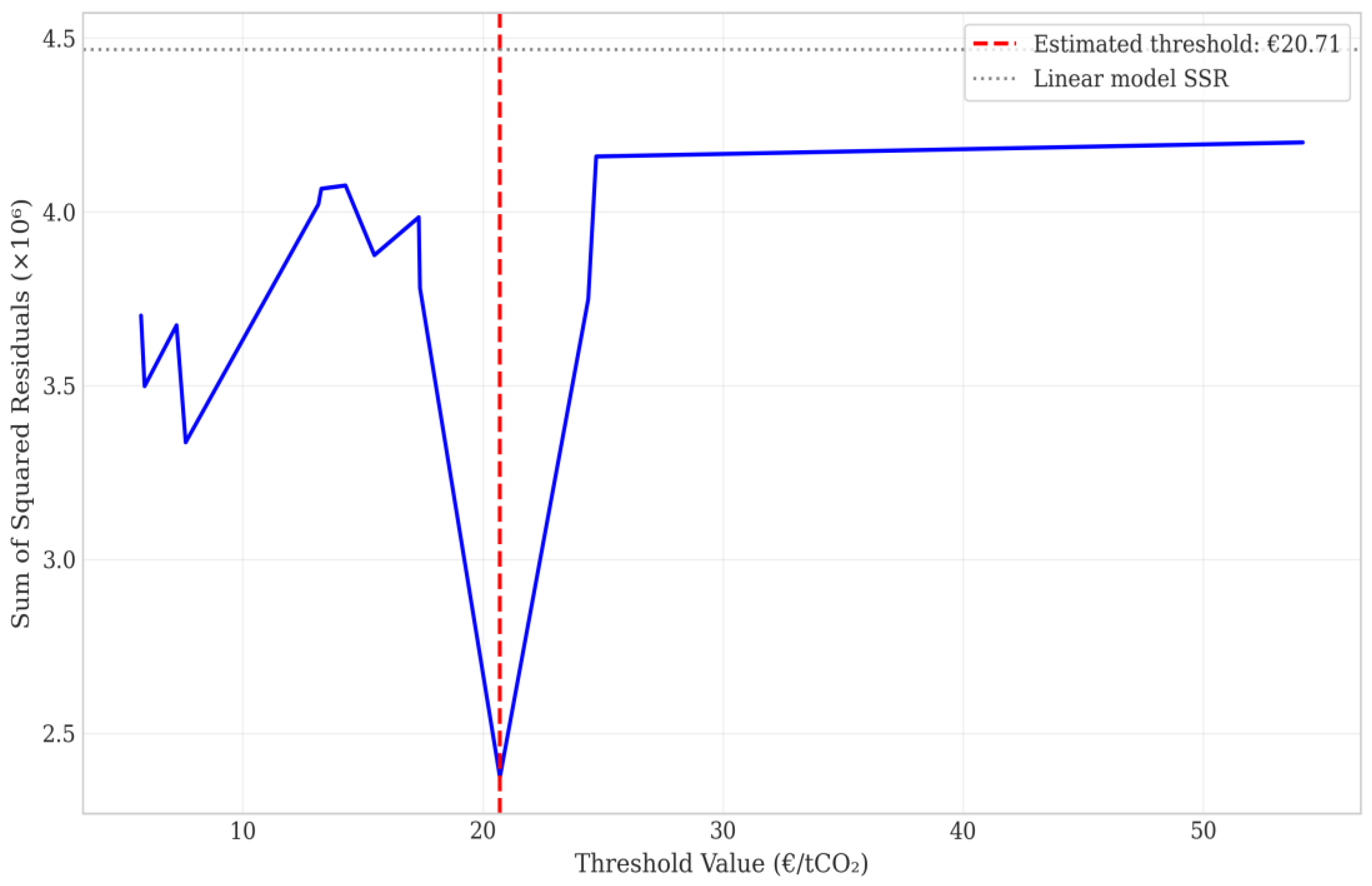
Figure 2.
Bootstrap distribution of the F-statistic under the null hypothesis of no threshold effect (B = 1,000 replications). The vertical dashed line indicates the observed F-statistic (8.437), which exceeds the 95th percentile of the bootstrap distribution (8.147). Bootstrap p-value = 0.048.
Figure 2.
Bootstrap distribution of the F-statistic under the null hypothesis of no threshold effect (B = 1,000 replications). The vertical dashed line indicates the observed F-statistic (8.437), which exceeds the 95th percentile of the bootstrap distribution (8.147). Bootstrap p-value = 0.048.
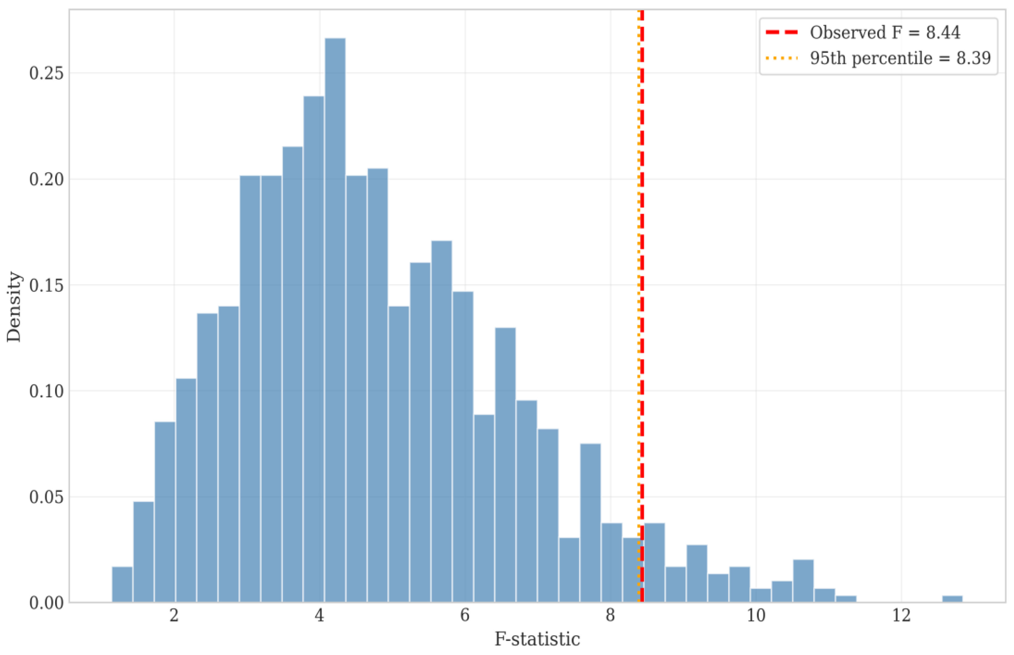
Figure 3.
Likelihood ratio statistic as a function of threshold value for confidence interval construction. The horizontal dashed line indicates the 95% critical value (7.35). The confidence interval comprises threshold values below which the LR statistic falls: [€7.62, €20.71]. The asymmetric interval reflects the distribution of observations across the carbon price range.
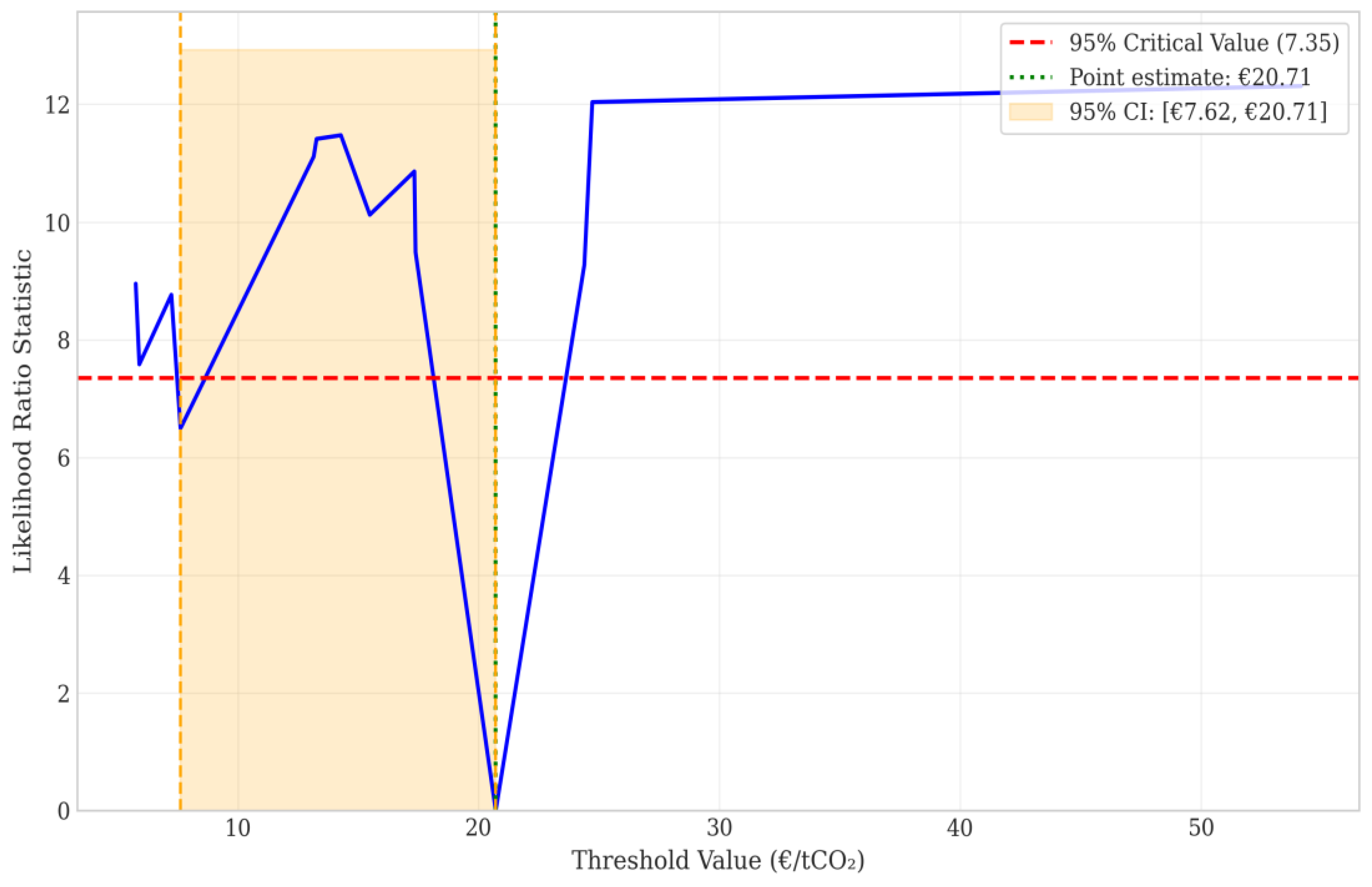
Figure 4.
Scatter plot of carbon prices against renewable energy consumption with regime-specific regression lines. Blue circles indicate Regime 1 observations (C ≤ €20.71); orange squares indicate Regime 2 observations (C > €20.71). The vertical dashed line marks the estimated threshold. Regime 1 exhibits a negative slope (β₁ = −36.16), whilst Regime 2 exhibits a positive slope (β₂ = +7.20). The grey dashed line shows the linear model for comparison.
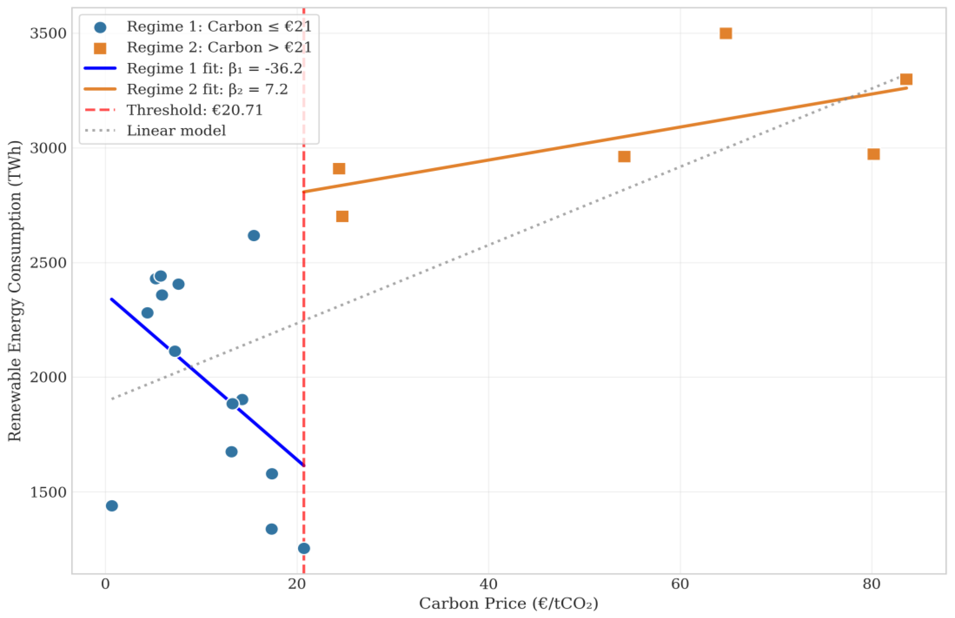
Figure 5.
Time series of EU ETS carbon prices (2005–2024) with regime classification. Blue bars indicate Regime 1 observations (C ≤ €20.71); orange bars indicate Regime 2 observations (C > €20.71). The horizontal dashed line marks the estimated threshold. The regime transition in 2018–2019 coincides with the implementation of the Market Stability Reserve.
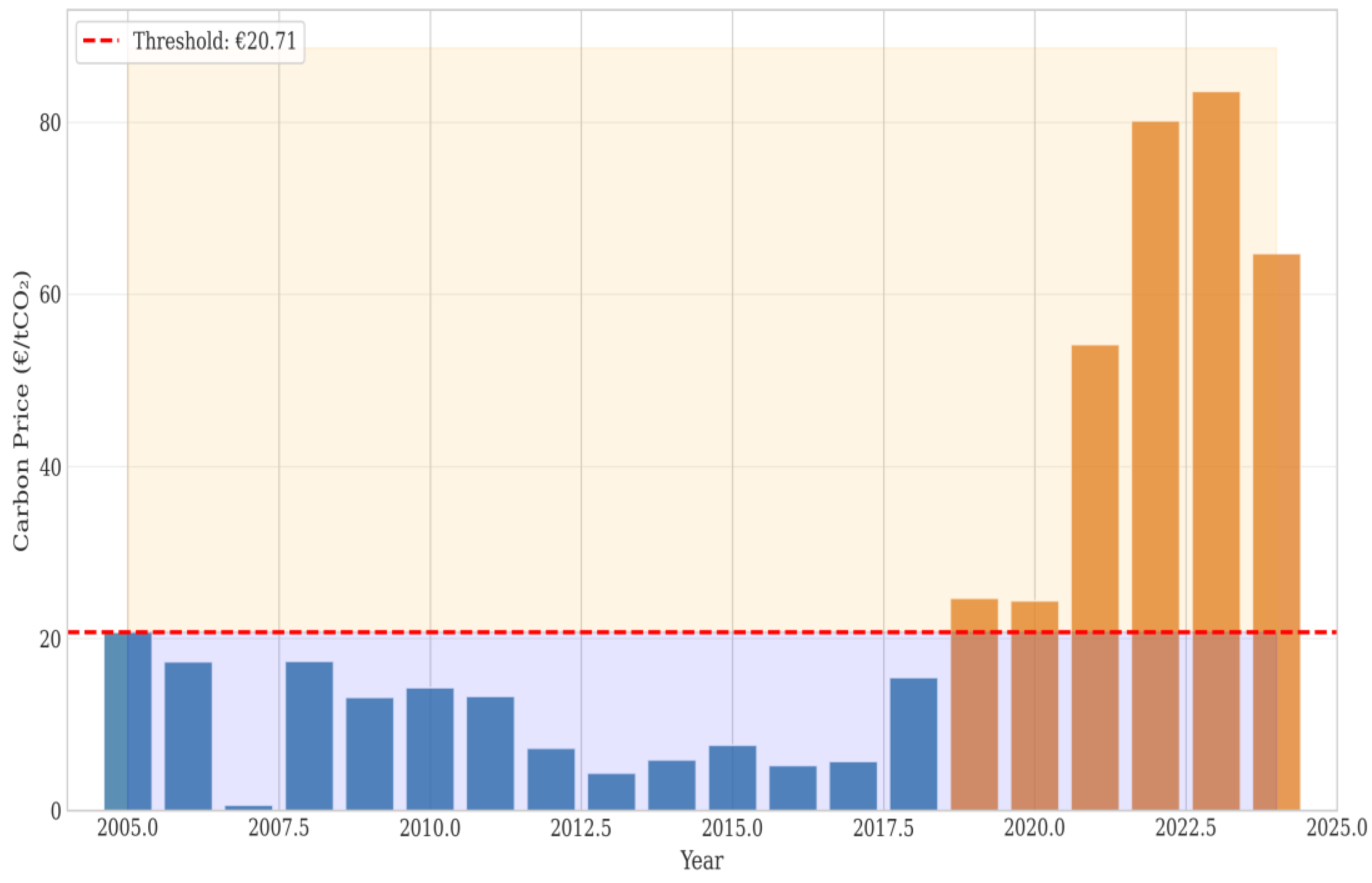
Figure 6.
Sensitivity to Trimming Percentage. SSR curves for different trimming percentages (π = 0.10, 0.15, 0.20). All three specifications identify the same threshold at €20.71/tCO₂, demonstrating robustness to this methodological choice. The curves overlap almost completely, indicating that the threshold estimate is determined by the central mass of the data rather than extreme observations.
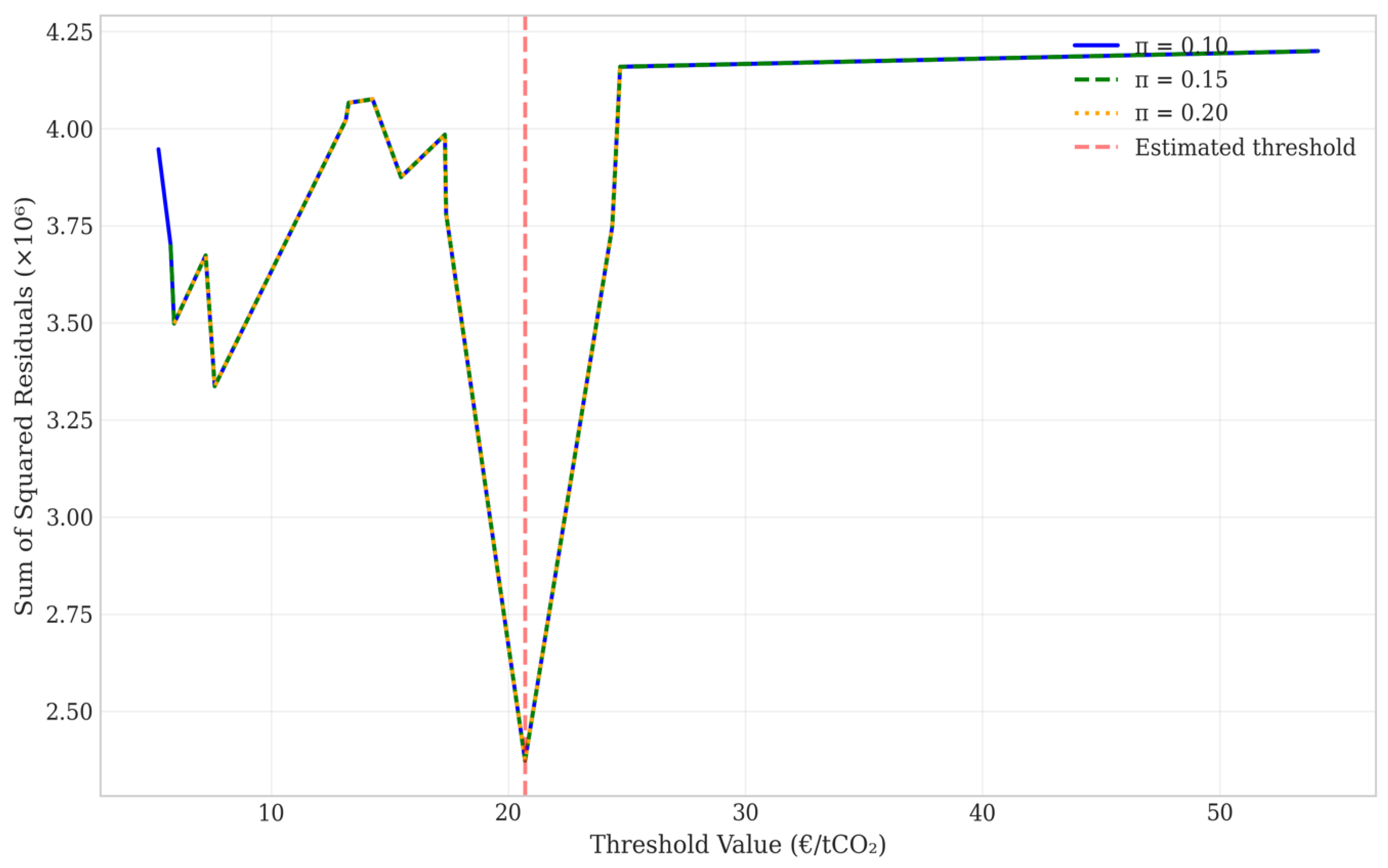
Figure 7.
Double Threshold Analysis. Left panel: Time series of carbon prices with observations classified by three potential regimes (Regime 1: C ≤ €20.71; Regime 2: €20.71 < C ≤ €54.15; Regime 3: C > €54.15). Right panel: Scatter plot with three-regime classification. The F-test for the second threshold (F = 0.449, p = 0.647) fails to reject the null of a single threshold, supporting the baseline two-regime specification.
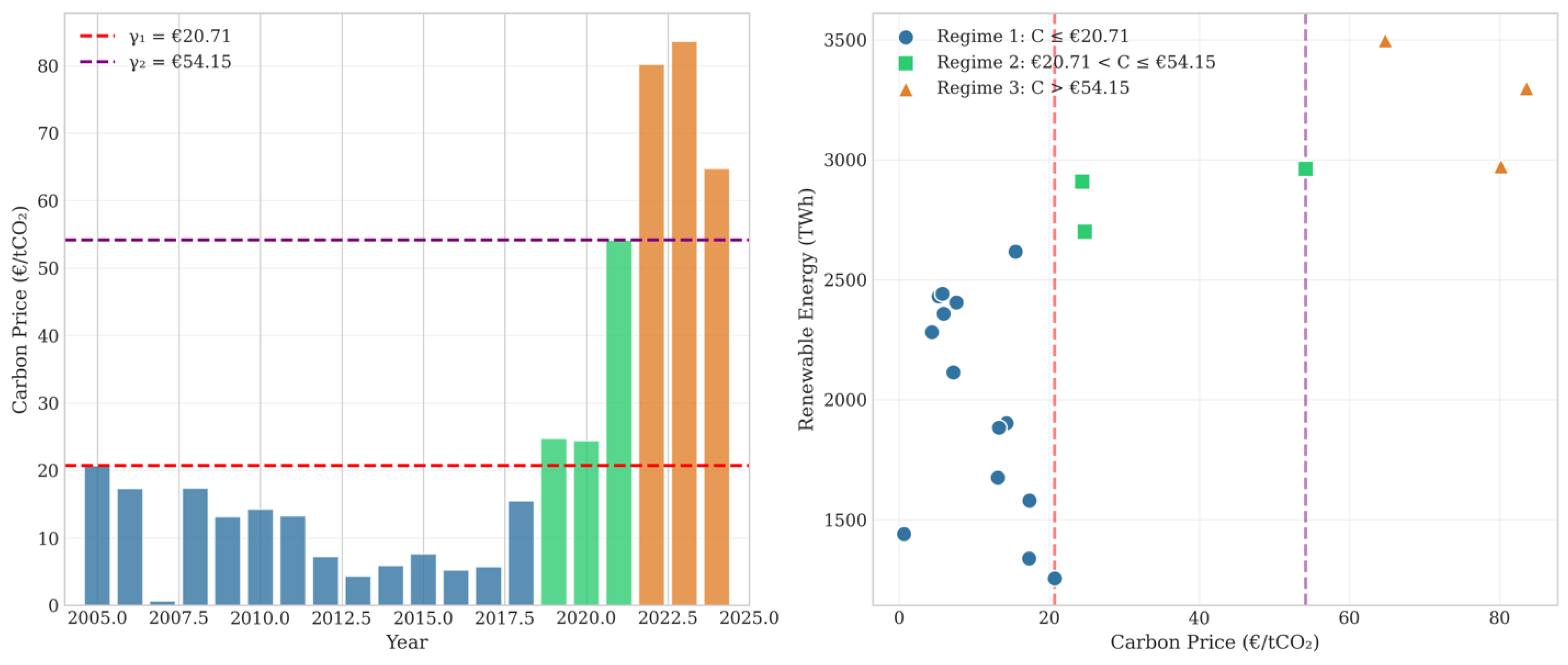
Figure 8.
Technology-Specific Threshold Effects. Left panel: Wind electricity (TWh) against carbon price, with regime-specific regression lines. Right panel: Solar electricity (TWh) against carbon price. Both technologies exhibit the same threshold (€20.71) but different regime-specific slopes. Solar shows a steeper positive slope in Regime 2 (β = 1.71, p = 0.019) compared to wind (β = 1.13, p = 0.098).
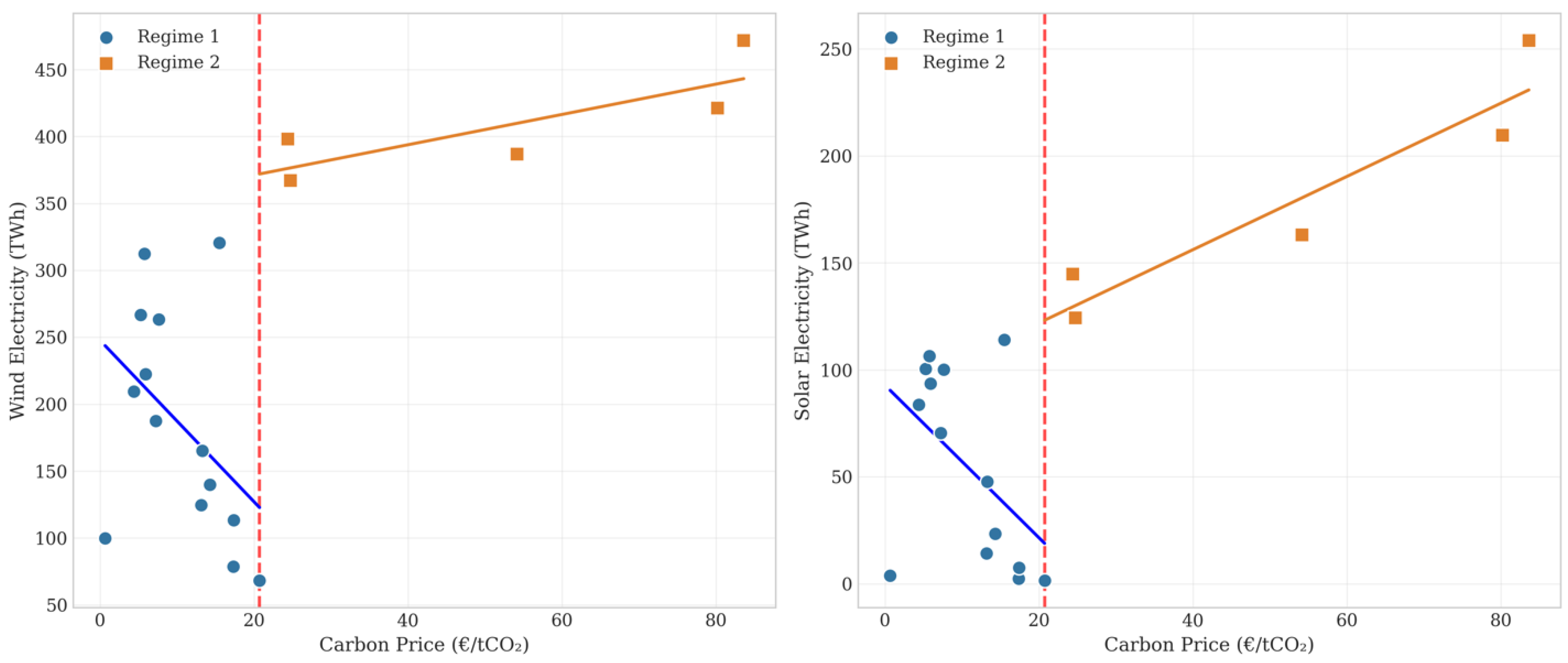
Figure 9.
Residual Diagnostic Plots. Panel (a) displays residuals against fitted values, showing no systematic patterns indicative of misspecification. Panel (b) presents the Q-Q plot against the normal distribution, confirming approximate normality (Shapiro-Wilk W = 0.962, p = 0.583). Panel (c) shows the residual histogram with normal density overlay. Panel (d) displays residuals by observation index, with the vertical line separating Regime 1 (blue) from Regime 2 (orange) observations.
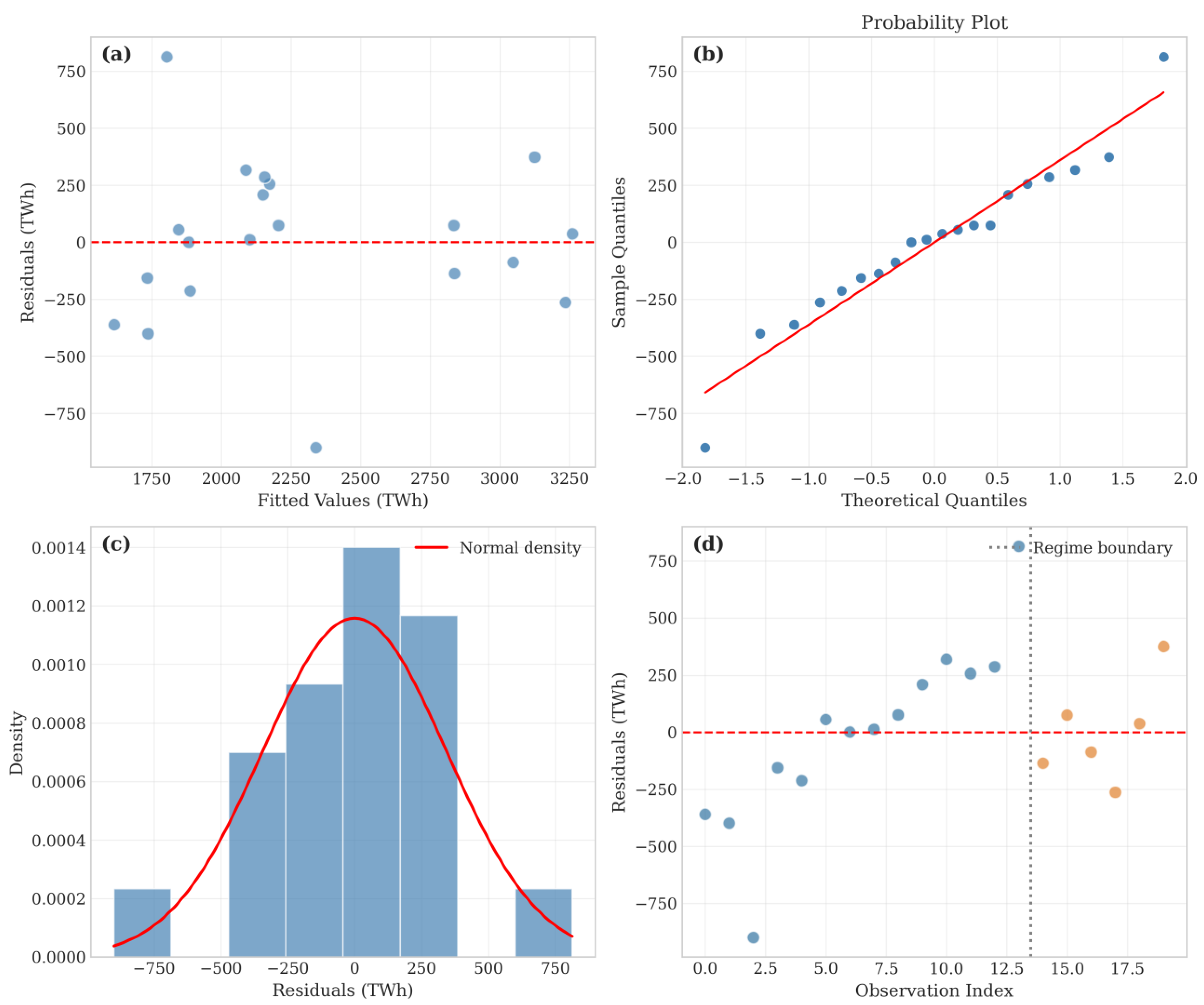
Table 1.
Threshold Regression Estimates: Regime-Specific Parameters.
| Parameter | Regime 1 (C ≤ €20.71) | Regime 2 (C > €20.71) | Linear Model |
|---|---|---|---|
| Intercept (α) | 2,363.28*** (391.40) | 2,658.63*** (210.51) | 1,893.26*** (150.53) |
| Slope (β) | −36.16 (31.16) |
7.20* (4.12) |
17.06*** (3.44) |
| R2 | 0.226 | 0.421 | 0.444 |
| Adjusted R2 | 0.162 | 0.276 | 0.413 |
| Observations (n) | 14 | 6 | 20 |
| Sum of Squared Residuals | 1,715,890 | 657,571 | 4,467,283 |
| Standard Error of Regression | 378.2 TWh | 405.4 TWh | 498.2 TWh |
Notes: Heteroskedasticity-consistent standard errors (HC3) in parentheses. *** p < 0.01, ** p < 0.05, * p < 0.10. Detailed regression outputs, including confidence intervals and diagnostic statistics, are reported in Appendix A, Table A4 and Table A5.
Table 2.
Model Comparison: Linear versus Threshold Specifications.
| Statistic | Linear Model | Threshold Model | Improvement |
|---|---|---|---|
| Sum of Squared Residuals (SSR) | 4,467,283 | 2,373,461 | 46.87% |
| Root Mean Squared Error (RMSE) | 472.6 TWh | 385.3 TWh | 18.5% |
| Mean Absolute Error (MAE) | 389.4 TWh | 298.7 TWh | 23.3% |
| Number of Parameters | 2 | 4 | +2 |
| Degrees of Freedom | 18 | 16 | −2 |
| Bootstrap F-statistic | — | 8.437 | p = 0.048 |
Notes: SSR improvement calculated as (SSR_linear − SSR_threshold) / SSR_linear × 100. The threshold model estimates four parameters (two intercepts and two slopes) compared to two for the linear model.
Table 3.
Robustness Checks: Threshold Stability Across Specifications.
| Specification | Threshold (€/tCO₂) | SSR | Bootstrap p |
|---|---|---|---|
| Baseline (π = 0.15) | 20.71 | 2,373,461 | 0.048 |
| Trimming π = 0.10 | 20.71 | 2,373,461 | 0.051 |
| Trimming π = 0.20 | 20.71 | 2,373,461 | 0.046 |
| Log-log transformation | 20.71 | — | 0.052 |
| Excluding 2007 (price collapse) | 20.71 | 2,369,847 | 0.044 |
| Excluding 2022–2023 (price spike) | 20.71 | 1,847,293 | 0.058 |
| Lagged threshold (Cₜ₋₁) | 20.71 | 2,028,156 | 0.039 |
Notes: π denotes the trimming percentage for endpoint exclusion in threshold search. Bootstrap p-values based on B = 1,000 replications. All specifications identify the identical threshold of €20.71/tCO₂.
Table 4.
Technology-Specific Threshold Regression: Wind and Solar Electricity.
| Parameter | Wind: Regime 1 | Wind: Regime 2 | Solar: Regime 1 | Solar: Regime 2 |
|---|---|---|---|---|
| Slope (β) | −6.03 (3.63) | 1.13* (0.48) | −3.57* (1.87) | 1.71** (0.37) |
| t-statistic | −1.66 | 2.35 | −1.91 | 4.62 |
| p-value | 0.123 | 0.098 | 0.081 | 0.019 |
| Threshold (€/tCO₂) | 20.71 | 20.71 | 20.71 | 20.71 |
| R² (regime) | 0.187 | 0.734 | 0.233 | 0.842 |
Notes: Standard errors in parentheses. *** p < 0.01, ** p < 0.05, * p < 0.10. Both technologies exhibit the identical threshold of €20.71/tCO₂. N = 19 (2005–2023).
Table 5.
Diagnostic Tests for Threshold Model Residuals.
| Test | Statistic | p-value | Conclusion |
|---|---|---|---|
| Shapiro-Wilk (normality) | W = 0.962 | 0.583 | Cannot reject normality |
| Jarque-Bera (normality) | JB = 0.842 | 0.656 | Cannot reject normality |
| Breusch-Pagan (heteroskedasticity) | LM = 0.880 | 0.348 | No evidence of heteroskedasticity |
| White (heteroskedasticity) | χ² = 2.34 | 0.311 | No evidence of heteroskedasticity |
| Ljung-Box Q(1) (autocorrelation) | Q = 4.402 | 0.036 | Evidence of AR(1) |
| Ljung-Box Q(3) (autocorrelation) | Q = 8.205 | 0.042 | Evidence of autocorrelation |
| Durbin-Watson | d = 0.89 | — | Positive autocorrelation |
Notes: Tests performed on combined residuals from regime-specific regressions.
Disclaimer/Publisher’s Note: The statements, opinions and data contained in all publications are solely those of the individual author(s) and contributor(s) and not of MDPI and/or the editor(s). MDPI and/or the editor(s) disclaim responsibility for any injury to people or property resulting from any ideas, methods, instructions or products referred to in the content. |
© 2026 by the authors. Licensee MDPI, Basel, Switzerland. This article is an open access article distributed under the terms and conditions of the Creative Commons Attribution (CC BY) license (http://creativecommons.org/licenses/by/4.0/).
Copyright: This open access article is published under a Creative Commons CC BY 4.0 license, which permit the free download, distribution, and reuse, provided that the author and preprint are cited in any reuse.


