
Submitted:
15 October 2025
Posted:
16 October 2025
You are already at the latest version
Abstract
The rapid rise of renewable generation has fundamentally altered electricity price dynamics, producing volatility and extreme events that classical stochastic models fail to capture. We develop and calibrate a semimartingale model that reproduces these new statistical realities of modern power markets. Using German EPEX SPOT data from 2015–2025, we document heavy-tailed, asymmetric Pareto-distributed price movements, frequent negative prices, and extreme volatility driven by renewable variability. Our model combines deterministic seasonality, mean-reverting diffusion, and compound Poisson jumps with asymmetric Pareto-distributed sizes, naturally accommodating negative prices without transformations. The calibrated process exhibits infinite variance for negative price excursions, reflecting the structural asymmetry between scarcity and oversupply events. Monte Carlo validation shows the model accurately reproduces key stylized facts—including bimodal negative price patterns, volatility clustering, and heavy-tailed extremes - where classical lognormal or Gaussian-based models fail. We derive futures pricing formulas consistent with the heavy-tailed structure and show analytically how volatility acts as a first-order cost driver in electricity markets through convexity effects, risk premiums, and system costs. The framework establishes a rigorous foundation for risk management and derivative valuation in electricity markets shaped by renewable volatility.
Keywords:
electricity spot prices
; renewable-driven volatility
; heavy-tailed distributions
; Pareto jumps
; semimartingale modeling
; sigma martingales
; EPEX SPOT Germany
; risk management
; futures pricing
; volatility-cost relationship
1. Introduction
The liberalization of electricity markets worldwide has created one of the most volatile and complex commodity markets, characterized by unique features that challenge traditional financial modeling approaches. Unlike storable commodities, electricity must be produced and consumed instantaneously, creating price dynamics fundamentally different from traditional financial assets. The integration of renewable energy sources over the past decade has further transformed these dynamics, introducing unprecedented volatility and regularly driving prices negative when renewable generation exceeds demand.
This paper develops a comprehensive stochastic model for electricity spot prices that captures the extreme statistical properties observed in modern power markets. Through extensive empirical analysis of German electricity spot prices from the EPEX SPOT exchange covering 2015-2025, we document several striking features that necessitate departures from standard modeling approaches. The coefficient of variation exceeds 2.4, far surpassing typical commodity markets where values rarely exceed 0.5 [104]. Prices regularly turn negative, occurring in 16.99% of 15-minute intervals, reflecting periods when generators pay consumers to take electricity due to inflexible baseload generation and high renewable output. Most critically, we find asymmetric heavy-tailed distributions with power-law indices of for positive price excursions and for negative excursions.
The empirical finding that has profound theoretical implications: it implies infinite variance for negative price movements, invalidating standard mean-variance approaches and requiring careful mathematical treatment through sigma-martingale theory. This heavy-tailed behavior is not merely a statistical curiosity but reflects fundamental market mechanics where oversupply conditions, constrained by must-run generation and limited storage, can create more extreme negative prices than scarcity creates positive prices.
Our contribution is threefold. First, we provide comprehensive empirical documentation of German electricity prices during a period of dramatic renewable expansion, revealing extreme statistical properties including tail indices approaching theoretical boundaries where moments become infinite. Second, we develop a semimartingale model combining mean-reverting diffusion with compound Poisson jumps following asymmetric Pareto distributions, demonstrating how this framework naturally accommodates negative prices and captures observed market dynamics. Third, we establish the mathematical foundations for pricing and risk management when classical assumptions fail, showing how sigma-martingale theory ensures arbitrage-free pricing even with infinite variance.
The model we propose belongs to the class of semimartingale processes and can be written as:
where captures deterministic seasonality through Fourier decomposition, follows an Ornstein-Uhlenbeck process representing normal fluctuations, and is a mean-reverting jump process with asymmetric Pareto-distributed jump sizes. This additive structure, aligned with recent advances by Aïd et al. [1], naturally accommodates negative prices without requiring artificial transformations like shifting or logarithmic modifications.
Our calibration results reveal important asymmetries in electricity markets. While jump frequencies are nearly balanced between positive and negative events (), the tail behavior differs dramatically. The negative tail index indicates that extreme negative price events follow a distribution so heavy-tailed that variance becomes infinite, while the positive tail with maintains finite second moments. This asymmetry emerges from fundamental market characteristics: when supply exceeds demand, the inability to store electricity combined with must-run constraints can drive prices arbitrarily negative, whereas positive price spikes are ultimately limited by demand destruction and emergency imports.
The theoretical implications extend beyond model specification to fundamental questions about market operation and risk management. We show that futures prices remain well-defined despite infinite spot price variance, deriving explicit pricing formulas under appropriate equivalent martingale measures. However, the heavy-tailed nature fundamentally alters risk management: traditional measures like Value-at-Risk converge slowly, variance-based portfolio optimization becomes inapplicable, and hedging strategies must account for potentially infinite hedge error variance.
Furthermore, we demonstrate that electricity’s extreme volatility is not merely a risk to be hedged but a fundamental cost driver. Through mathematical analysis and empirical evidence, we show how volatility increases average prices through multiple channels: Jensen’s inequality effects from convex supply curves, risk premiums in forward contracts, expensive reserve requirements, and elevated hedging costs. These findings have important policy implications, suggesting that investments in storage, demand response, and grid flexibility could significantly reduce electricity costs by dampening volatility.
The remainder of this paper is organized as follows. Section 2 presents our comprehensive empirical analysis of German electricity spot prices. Section 3 develops the theoretical model and discusses its mathematical properties. Section 4 addresses the embedding in a general semimartingale framework and derives futures pricing results. Section 5 presents model calibration and validation through Monte Carlo simulation. Section 6 analyzes how volatility drives electricity costs. Section 7 concludes.
2. Empirical Analysis of German Electricity Spot Prices
The European electricity market represents one of the most complex and dynamic commodity markets globally, characterized by the unique non-storability of electricity and the requirement for instantaneous supply-demand balance [46,124]. Unlike traditional commodity markets, electricity markets operate through a sequence of interconnected trading venues, from long-term bilateral contracts to day-ahead auctions and real-time balancing markets [62]. The fundamental constraint that supply must equal demand at every moment, combined with transmission network limitations and regulatory frameworks, creates a market structure fundamentally different from other commodities [22].
The integration of renewable energy sources has dramatically transformed electricity market dynamics over the past decade [79,128]. Wind and solar generation, characterized by their intermittent and weather-dependent nature, introduce unprecedented volatility into the system [59,108]. This volatility manifests not only in price fluctuations but also in the frequency of extreme events, including negative prices when renewable generation exceeds demand and system flexibility [48,109]. The German market, with its aggressive renewable energy targets under the Energiewende policy, experiences particularly extreme price dynamics [51,57].
The interconnected nature of European electricity markets adds another layer of complexity through cross-border flows and market coupling mechanisms [78,101]. While market integration theoretically improves efficiency and security of supply, it also transmits volatility and extreme events across borders [58]. Germany’s central position in the European grid and its high renewable penetration make it a critical node for understanding modern electricity market dynamics [68].
We focus our empirical analysis on the German electricity market, specifically the EPEX SPOT exchange, which exhibits some of the most extreme price behavior globally [80,100]. The German market regularly experiences both extreme positive spikes and negative prices, making it an ideal laboratory for studying electricity price dynamics under high renewable penetration [54,99].
2.1. Data Description and Basic Statistics
Our dataset comprises spot prices from the German-Luxembourg bidding zone obtained through the ENTSO-E Transparency Platform API, covering the period from January 1, 2015, to June 1, 2025. The data represents day-ahead auction results from EPEX SPOT at 15-minute resolution. We obtain 15-minute EPEX SPOT day-ahead prices and resample to hourly means for the empirical analysis; let T denote the resulting number of hourly observations over this sample period. This publicly available data captures the evolution of prices through significant structural changes in the German electricity system, including the phase-out of nuclear power and rapid expansion of renewable capacity [71].
It is important to note that while current EPEX SPOT day-ahead markets operate with harmonized price bounds (floor of -500 EUR/MWh and cap of 5,000 EUR/MWh as of September 20, 2022), our dataset includes historical periods before these constraints were uniformly implemented. Prior to the harmonization of price caps across European markets, extreme price excursions beyond current limits were possible during exceptional market conditions. Additionally, data anomalies from the aggregation process or reporting errors may contribute to outliers that require careful treatment in the analysis.
From a modeling perspective, we deliberately choose not to incorporate price bounds in our theoretical framework. Price caps and floors, while important for market operations, distort the true interaction of supply and demand forces that drive electricity prices. To understand the fundamental market dynamics and extreme event probabilities, it is essential to model the unbounded price process that would emerge from physical and economic constraints alone. The presence of pre-harmonization data in our sample, where prices could exceed current bounds, provides valuable information about tail behavior under extreme market stress. This unconstrained data allows us to calibrate models that capture the true severity of supply-demand imbalances, which is crucial for risk management and understanding the economic value of flexibility resources. Artificial truncation at regulatory bounds would underestimate tail risks and obscure the underlying economic signals that prices convey about system scarcity.
Understanding the basic statistical properties of electricity prices is fundamental for model selection and risk management [89]. The first two moments provide information about the central tendency and dispersion, while higher moments reveal the asymmetry and tail behavior crucial for extreme event modeling. For our hourly aggregated data, we calculate the sample moments as:
where denotes the spot price at time t, and T is the total number of hourly observations.
The statistics in Table 1 reveal several striking features. The coefficient of variation of 2.444 indicates volatility far exceeding typical commodity markets, where values rarely exceed 0.5 [104]. The extreme skewness and kurtosis values indicate severe departures from normality, necessitating models that can capture both frequent small variations and occasional extreme events [96]. However, it should be noted that these extreme values for higher-order moments are dominated by the rare extreme observations that exceed current market bounds, and robust estimation methods might yield more stable estimates.
The distinction between 15-minute and hourly negative price frequencies is particularly important: while 16.99% of 15-minute intervals show negative prices, only 8.47% of hourly averages are negative, demonstrating the impact of temporal aggregation on price statistics. The difference illustrates aggregation effects: averaging four quarter-hour prices materially lowers the frequency of negative hourly values. This high frequency of negative prices reflects periods when generators pay consumers to take electricity due to inflexible baseload generation and high renewable output [21].
Figure 1 illustrates the characteristic behavior of electricity spot prices through three 30-day sample paths. The extreme volatility is immediately apparent, with prices ranging from negative values to spikes exceeding 2000 EUR/MWh. The zoomed view in the lower panel provides a comprehensive view of price dynamics, showing the mean-reverting nature of the price process, with excursions from the mean being followed by rapid returns to normal levels [11].
2.2. Annual Seasonality Removal
Before analyzing the structural properties of electricity prices, it is essential to remove long-term seasonal patterns that could confound the estimation of mean reversion, jump dynamics, and other structural parameters. We employ STL (Seasonal and Trend decomposition using Loess) decomposition to extract the annual seasonal component:
where represents the long-term trend, is the annual seasonal component, and contains the remaining dynamics including intraday patterns, jumps, and stochastic variations.
We estimate the annual component via STL with period 8760 (hours in a non-leap year) and subtract it from the hourly series to obtain deseasonalized prices:
This approach is robust to outliers and missing values, using the iterative loess smoothing inherent in the STL algorithm. The method effectively separates annual patterns from shorter-term dynamics while preserving the essential statistical properties of the price series.
The decomposition results shown in Figure 2 reveal a modest annual seasonal pattern with a range of approximately 42.24 EUR/MWh. The seasonal strength metric of 0.001 indicates that annual seasonality explains only 0.1% of the total variance, confirming that short-term volatility dominates the price dynamics. This weak annual seasonality is characteristic of electricity markets where weather-dependent demand and supply patterns are overlaid with substantial noise from market dynamics, fuel price variations, and renewable generation variability [122].
The deseasonalized data retains the essential statistical properties: mean of 58.76 EUR per MWh (compared to 58.16 for raw data) and standard deviation of 142.04 EUR/MWh (compared to 142.12). For context, in the underlying quarter-hour series, the negative price frequency changes marginally from 16.99% to 17.76% after deseasonalization, while the hourly aggregated series shows a similar modest change. The minimal impact on these statistics confirms that annual seasonality removal does not distort the fundamental price dynamics while providing cleaner estimates of structural parameters.
2.3. Fourier Decomposition of Intraday and Weekly Patterns
To capture the regular intraday and weekly patterns in electricity prices, we apply Fourier decomposition to the deseasonalized data. Following Geman and Roncoroni [53], we model the deterministic seasonal component as:
where is the base level, denotes the hour of day, and are the number of harmonics for daily and weekly patterns respectively, and the coefficients are estimated using least squares on the deseasonalized data aggregated to hourly resolution.
The Fourier decomposition shown in Figure 3 successfully captures the periodic patterns with high fidelity. The intraday pattern exhibits the characteristic double-peak structure with morning peaks around 8-9 AM and evening peaks around 6-8 PM, with a peak/off-peak ratio of 1.35. The R² of 0.943 for the intraday fit confirms that three harmonics adequately capture the daily variation. The weekly pattern shows lower prices on weekends, with Sunday having the lowest average prices. The estimated Fourier coefficients are presented in Table 2.
2.4. Log Returns Analysis
The analysis of price changes through log returns provides insights into the dynamic behavior of electricity prices and is essential for volatility modeling and derivative pricing [125]. For positive prices, log returns are defined as:
However, the presence of negative prices in electricity markets requires a modification to the standard approach. Following [109], we employ the generalized logarithm transformation:
This transformation preserves the sign of prices while maintaining the desirable properties of log returns for large price movements.
The distributional analysis of returns is crucial for understanding price dynamics and selecting appropriate stochastic models. We test for normality using the Jarque-Bera statistic:
where represents the null hypothesis of normality. For the hourly log returns with T observations, the computed skewness of 0.020 and excess kurtosis of 4.451 yield a Jarque-Bera statistic that decisively rejects normality, providing evidence of heavy-tailed behavior in electricity returns.
The log returns analysis in Figure 4 reveals several important stylized facts. The distribution exhibits significant excess kurtosis (4.451) indicating heavy tails, while maintaining near-zero skewness (0.020). The Jarque-Bera test strongly rejects normality (p-value < 0.001), consistent with findings in electricity price literature [96]. The QQ-plot shows systematic deviations from normality, particularly in the tails, suggesting the presence of jumps or extreme events that cannot be captured by continuous diffusion models [27].
The autocorrelation function (ACF) of log returns shows rapid decay, indicating limited linear dependence. However, this does not imply independence, as evidenced by the significant autocorrelation in squared returns shown in Figure 5. This pattern is characteristic of GARCH-type effects and motivates the use of stochastic volatility models [83].
2.5. Volatility Clustering Analysis
Volatility clustering, where large price changes tend to be followed by large changes of either sign, is a ubiquitous feature of commodity markets [90]. For electricity prices, this phenomenon is particularly pronounced due to the interaction between weather-dependent supply and demand, planned maintenance, and unexpected outages [77].
We analyze volatility clustering through the autocorrelation function of squared returns:
Additionally, we compute time-varying volatility using a rolling window approach:
with hours (one week) to capture weekly patterns while maintaining sufficient responsiveness.
Figure 5 demonstrates strong evidence of volatility clustering. The ACF of squared returns shows significant autocorrelation with slow decay (Ljung-Box test p-value < 0.001 for lags up to 200), indicating that volatility shocks persist for extended periods. The autocorrelation at lag 1 is approximately 0.31, indicating that volatility shocks have a persistence measure corresponding to roughly 31% correlation after one hour. This persistence of volatility - distinct from the mean reversion of price levels - reflects the physical constraints and operational characteristics of electricity systems [53]. The time-varying volatility plot reveals distinct regimes, with particularly elevated volatility during 2021-2022 corresponding to the European energy crisis. The volatility ranges from below 1 during calm periods to over 5 during crisis periods, representing a five-fold increase that has important implications for risk management and derivative pricing [10].
2.6. Structural Parameter Estimation
To estimate the structural parameters of electricity price dynamics, we analyze the deseasonalized data to separate the effects of mean reversion, jumps, and stochastic volatility from seasonal patterns. This approach provides cleaner estimates of the fundamental price dynamics.
2.6.1. Mean Reversion
The mean reversion rate is estimated from the autocorrelation function of deseasonalized prices aggregated to hourly resolution:
where ACF(1) denotes the first-order autocorrelation. For the deseasonalized hourly data, we obtain per hour, corresponding to a half-life of hours. Because jumps add short-lag dependence, should be read as an OU-equivalent mean-reversion speed - the rate that would generate the same first-order autocorrelation in a pure Ornstein-Uhlenbeck process. This rapid mean reversion reflects the inability to store electricity and the requirement for continuous supply-demand balance.
2.6.2. Jump Parameters
Jump detection on deseasonalized data uses a rolling window approach to identify extreme deviations:
where and are the rolling mean and standard deviation over a weekly window (168 hours for hourly data). The analysis on hourly aggregated data identifies 3,908 jumps over the sample period, yielding a jump intensity of . The ratio of negative to positive jumps is , indicating a slight bias toward negative jumps, consistent with the asymmetric response of electricity systems to supply and demand shocks.
Figure 6.
Structural parameter estimation results. Top left: ACF of deseasonalized prices with exponential decay fit. Top right: Jump detection on deseasonalized data. Bottom left: ACF of squared returns showing volatility clustering. Bottom right: Summary of structural parameter estimates.
Figure 6.
Structural parameter estimation results. Top left: ACF of deseasonalized prices with exponential decay fit. Top right: Jump detection on deseasonalized data. Bottom left: ACF of squared returns showing volatility clustering. Bottom right: Summary of structural parameter estimates.
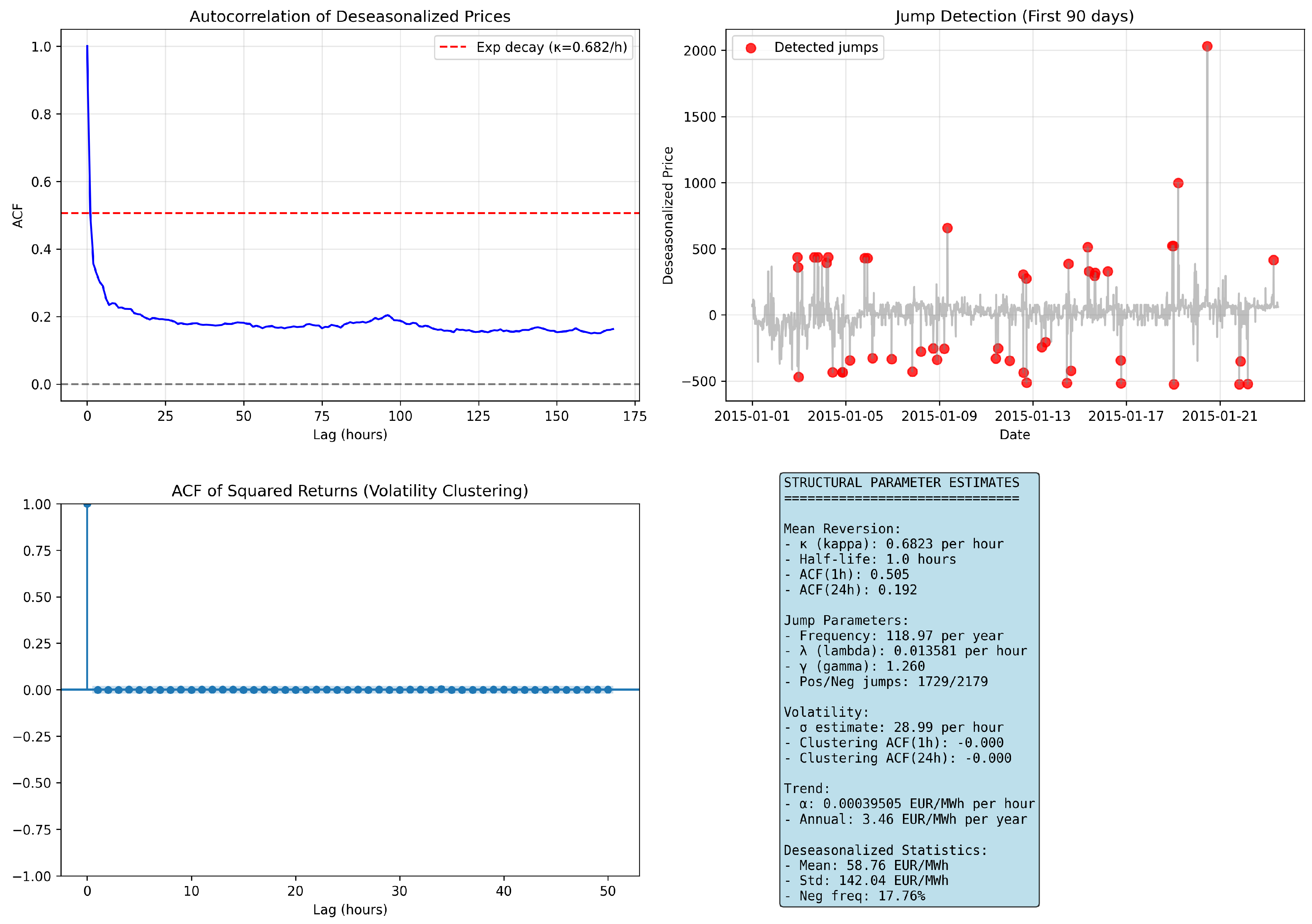
2.6.3. Trend Analysis
Long-term trends in electricity prices reflect fundamental changes in the generation mix, fuel costs, environmental regulations, and market structure [113]. We estimate the trend parameter using linear regression on deseasonalized data:
The estimated trend is EUR/MWh per hour, or 3.46 EUR/MWh per year. The Kendall rank correlation test confirms the statistical significance of this trend (, p-value < 0.001).
2.7. Periodicity and Spectral Analysis
Electricity demand, and consequently prices, exhibit strong periodic patterns driven by human activity cycles [33]. Understanding these patterns is crucial for forecasting and operational planning. We analyze periodicity using spectral methods, which decompose the price series into frequency components.
The periodogram provides a non-parametric estimate of the power spectral density:
where is the centered price series and are the Fourier frequencies.
For improved estimates, we employ Welch’s method [120], which averages periodograms of overlapping segments:
where is the periodogram of the k-th windowed segment.
The spectral analysis in Figure 7 reveals a rich periodic structure. The power spectrum exhibits clear peaks at frequencies corresponding to 24-hour (daily) and 168-hour (weekly) cycles, with the daily frequency showing the strongest signal. The spectrum shows strong peaks at daily and weekly cycles. The low-frequency slope indicates persistent correlation at multi-day scales, while the high-frequency decay ( with ) reflects short-horizon roughness characteristic of electricity prices [8]. Additional peaks at harmonics of the fundamental frequencies (12 hours, 8 hours, 6 hours) reflect the multi-peaked nature of daily demand patterns.
The autocorrelation function provides complementary evidence, with significant correlations at lags of 24, 48, and 168 hours persisting even after 7 days. This persistent correlation structure has important implications for time series modeling, suggesting that models must incorporate both short-term dynamics and long-term periodic components [122].
2.8. Daily Seasonal Decomposition
To analyze the short-term seasonal patterns in detail, we apply STL (Seasonal and Trend decomposition using Loess) [32] with a daily period. This decomposition separates the intraday patterns from longer-term dynamics:
where is the trend component, is the 24-hour seasonal component, and is the remainder. The decomposition uses locally weighted regression (loess) to extract components iteratively.
The strength of the daily seasonality can be quantified as:
The STL decomposition in Figure 8 successfully separates the different price components on a daily basis. The seasonal component exhibits a clear 24-hour pattern with amplitude of approximately ±15 EUR/MWh, representing about 25% of the mean price. The visualization shows 30 days of the seasonal pattern to better illustrate its consistency across multiple weeks. The seasonal strength metric indicates that daily seasonality explains 73% of the detrended variance, confirming its importance in price formation. The residual component contains the irregular price movements, including spikes and drops, which require separate modeling approaches [72].
2.9. Intraday and Weekly Patterns
The regular patterns in electricity prices reflect the underlying patterns in electricity demand and supply availability. We analyze these patterns by computing conditional statistics:
for hourly patterns, and similarly for day-of-week effects.
The seasonal analysis in Figure 9 reveals several important patterns. The intraday profile shows the characteristic double-peak structure, with morning peaks around 8-9 AM (mean price 65 EUR/MWh) and evening peaks around 6-8 PM (mean price 70 EUR/MWh). Off-peak hours (2-5 AM) average 45 EUR/MWh, creating a peak/off-peak ratio of approximately 1.35. The standard deviation also varies systematically, being highest during peak hours when system constraints are most likely to bind.
Weekly patterns show significantly lower prices on weekends (average 48 EUR/MWh) compared to weekdays (average 62 EUR/MWh), reflecting reduced industrial demand. The hour-day heatmap reveals that Sunday nights have the lowest prices, while Wednesday and Thursday evenings show the highest prices, consistent with industrial production patterns in Germany [68].
Particularly revealing is the distribution of negative prices by hour, calculated from our 15-minute data. Negative prices occur most frequently during night hours (1-5 AM) with frequencies exceeding 20% of 15-minute intervals, and during midday hours (11 AM - 3 PM) with frequencies around 18%. This bimodal pattern reflects two different mechanisms: nighttime negative prices result from inflexible baseload generation during low demand, while midday negative prices occur during high solar production [99].
2.10. Spike Analysis
Price spikes represent extreme deviations from normal price levels and pose significant risks for market participants [30]. We define spikes as extreme price levels identified using a dynamic threshold approach based on rolling statistics:
where and are rolling mean and standard deviation over window hours, and is the threshold parameter.
The spike analysis in Figure 10 identifies 3,405 spike events (extreme price levels) over the sample period (approximately 10.4 years), split between 1,529 positive spikes and 1,876 negative spikes. This corresponds to approximately 327 spikes per year or 0.89 spikes per day, indicating that extreme price levels are a regular feature of the German electricity market rather than rare occurrences.
The spike magnitude distribution follows a power law in the tails:
with estimated tail index for both positive and negative spikes. The inter-arrival time analysis reveals that spikes do not occur uniformly in time. The distribution of waiting times between spikes follows approximately an exponential distribution with rate parameter days, but with excess probability at short intervals indicating clustering. This clustering effect reflects the persistence of system stress conditions [53].
2.11. Jump Analysis
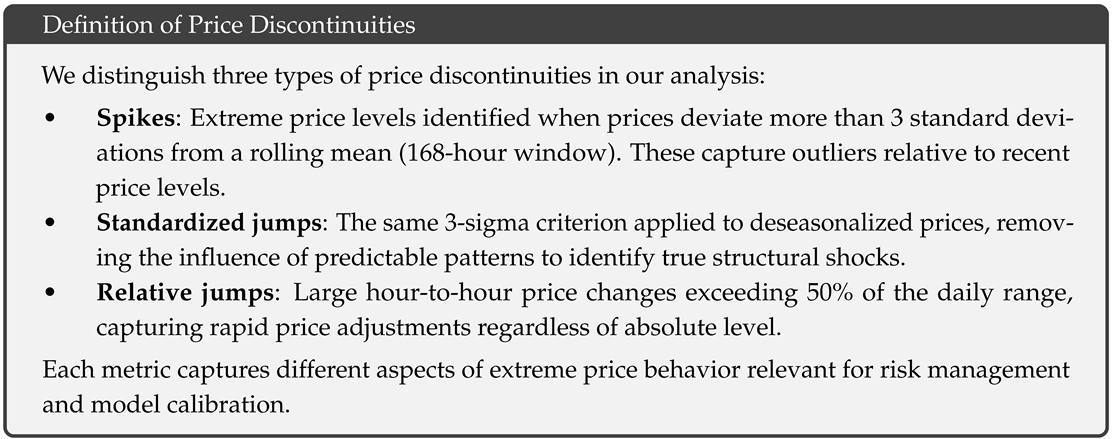
While spikes represent extreme price levels, jumps capture rapid price changes that may indicate system shocks or information arrival [20]. We now analyze each of the three discontinuity metrics from the definition box:
Standardized jumps: Identified on deseasonalized data using a rolling window approach:
where and are the rolling mean and standard deviation over a weekly window (168 hours). This method identifies 3,908 standardized jumps over the sample period, yielding a jump intensity of (approximately 119 jumps per year).
Relative price jumps: Identified using the relative price change criterion:
where is the daily price range and is the threshold parameter.
The relative jump analysis in Figure 11 identifies 9,771 significant price changes over the sample period, with a remarkably balanced distribution between positive (50.3%) and negative (49.7%) jumps. This corresponds to approximately 2.56 relative jumps per day, reflecting rapid hour-to-hour price adjustments. The average jump magnitudes are 265.6 EUR/MWh for positive jumps and 272.7 EUR/MWh for negative jumps, with standard deviations exceeding the means, confirming the heavy-tailed nature of jump sizes.
The distinction between standardized jumps (119 per year) and relative price jumps (2.56 per day) reflects different aspects of price dynamics: standardized jumps capture departures from the rolling mean (level outliers), while relative jumps capture large hour-to-hour changes regardless of the prevailing price level. Both metrics provide important calibration targets for jump models.
Crucially, our jump-scale metrics reveal important calibration parameters for theoretical models:
The near-unity jump magnitude ratio of 0.97 indicates that positive and negative jumps have remarkably similar average sizes, despite their different underlying causes. This symmetry in jump magnitudes, combined with the slight asymmetry in frequency ( for standardized jumps), provides key calibration targets for jump models. The values of and EUR/MWh represent the characteristic scale of extreme price movements and can be interpreted as the minimum jump sizes in Pareto-based jump models. We use Pareto Type-I tails above thresholds ; setting would make the Lévy measure non-integrable.

Table 3.
Jump-Scale Metrics
| Parameter | Value |
|---|---|
| (mean positive jump) [] | 265.65 |
| (mean negative jump) [] | 272.73 |
| Jump magnitude ratio | 0.97 |
The distribution of daily jump counts deviates from the Poisson model, showing excess probability for days with multiple jumps. This clustering of jumps within days reflects the fact that system stress conditions often persist for several hours, leading to multiple price adjustments [60].
2.12. Extreme Value Analysis
Understanding the tail behavior of electricity prices is crucial for risk management and system reliability assessment. We employ extreme value theory to characterize the distribution of extreme prices, with particular focus on the asymmetry between positive and negative tails.
For tail analysis, we employ both the Hill estimator and maximum likelihood estimation (MLE) as a fallback for robust estimation of the tail index. The tail behavior is characterized by the Pareto distribution:
where u is the threshold and is the tail index.
The tail analysis in Figure 12 reveals significant asymmetry in extreme value behavior. The positive tail exhibits an empirical tail index of , while the negative tail shows a substantially heavier tail with empirical . For model calibration purposes, we obtain calibrated indices and . This asymmetry has important economic implications: while positive price spikes are limited by demand response and the availability of peaking generation, negative prices can become extremely negative when renewable generation far exceeds demand and system flexibility is exhausted [31].
The Hill plots in Figure 13 confirm stable tail index estimates above the selected thresholds. The heavier negative tail () indicates that extreme negative price events are more likely than comparably extreme positive events, reflecting the fundamental asymmetry in electricity markets where excess generation is harder to manage than shortages [130].
2.13. Additional Trend Diagnostics
Beyond the primary trend analysis, we examine medium-term cycles and inter-annual variability to understand the evolution of electricity markets under structural changes.
The trend analysis in Figure 14 reveals a statistically significant upward trend of 3.46 EUR/MWh per year (Kendall’s , p-value < 0.001). This trend reflects multiple factors including the phase-out of nuclear power, increasing carbon prices under the EU ETS, and the costs of renewable integration [65]. However, the R-squared value of 0.053 indicates that the linear trend explains only 5.3% of price variation, emphasizing the dominance of short-term volatility over long-term trends.
The 365-day rolling average reveals important medium-term cycles superimposed on the long-term trend. Notable features include the price collapse during the COVID-19 pandemic in 2020, followed by the dramatic spike during the 2021-2022 energy crisis when gas supply constraints and low renewable output combined to create extreme scarcity [129]. The detrended series maintains substantial volatility, confirming that trend removal does not eliminate the extreme price behavior characteristic of electricity markets.
2.14. Summary and Implications
Our comprehensive empirical analysis of German electricity spot prices reveals a market characterized by extreme complexity and unprecedented volatility. The key findings can be summarized as follows:
First, German electricity prices exhibit volatility levels far exceeding other commodity markets, with a coefficient of variation of 2.444. The presence of extreme outliers, some of which exceed current market bounds and likely represent data anomalies or historical periods before cap implementation, significantly affects statistical measures, particularly higher-order moments. The tail analysis reveals asymmetric heavy-tailed distributions with empirical tail indices of for positive tails and for negative tails, necessitating careful treatment of extreme observations in empirical work.
Second, the distinction between 15-minute and hourly data resolution is crucial for accurate analysis. Our dataset contains observations at 15-minute resolution, which when aggregated to hourly data yields different statistics. Notably, 16.99% of 15-minute intervals (but only 8.47% of hourly averages) are negative, demonstrating the impact of temporal aggregation on market statistics.
Third, the price dynamics combine multiple temporal scales: high-frequency noise with rapid mean reversion ( per hour when estimated from hourly data), regular daily and weekly seasonality captured by Fourier decomposition (R² = 0.943 for intraday patterns), modest annual seasonality (0.1% of variance), and long-term trends of 3.46 EUR/MWh per year. The spectral analysis reveals that these components interact in complex ways, with volatility clustering persisting for extended periods.
Fourth, extreme events in the form of spikes and jumps are regular features of the market. We identify three types of discontinuities: level spikes (approximately 327 per year or 0.89 per day), standardized jumps on deseasonalized data (119 per year), and relative price jumps (2.56 per day). The jump-scale metrics reveal characteristic magnitudes of EUR/MWh for positive jumps and EUR/MWh for negative jumps, with a near-unity magnitude ratio of 0.97. The heavy-tailed distribution of these events, particularly for negative prices with , implies that risk measures based on normal distributions severely underestimate the true risks in electricity markets.
These findings have important implications for market participants and policymakers. For traders and risk managers, the structural parameter estimates provide essential inputs for stochastic models: mean reversion rate per hour (from hourly data), level spikes at 327 per year (0.89/day), standardized jump intensity (≈ 119/year), relative jumps at 2.56 per day, negative-to-positive jump ratio , asymmetric empirical tail indices and , and jump-scale parameters and EUR/MWh. The Fourier coefficients enable accurate modeling of intraday and weekly patterns crucial for short-term forecasting and trading strategies.
For system operators, the increasing frequency of extreme prices signals growing system stress that may require new flexibility resources or market design changes. The bimodal distribution of negative prices - occurring both at night and midday - highlights the dual challenges of inflexible baseload generation and high solar penetration.
For policymakers, the analysis highlights both the achievements and challenges of the energy transition. While renewable integration has been successful, it has created new forms of price risk that must be managed. The asymmetric tail behavior suggests that market rules may need to differentiate between positive and negative price extremes.
The German experience provides valuable lessons for other markets following similar renewable integration paths. As renewable penetration increases globally, the extreme price dynamics observed in Germany may become the new normal rather than the exception, requiring fundamental changes in how electricity markets are designed, operated, and regulated.
3. Theoretical Model for Electricity Spot Prices
3.1. Literature Review and Modeling Approaches
The modeling of electricity spot prices has evolved significantly since market deregulation began in the 1990s, driven by the unique characteristics that distinguish electricity from other commodities. The non-storability of electricity, combined with inelastic short-term demand and supply constraints, creates price dynamics fundamentally different from traditional financial assets [23,89].
Early approaches adapted models from financial mathematics, whereas Schwartz [112] proposed mean-reverting diffusion processes for commodity prices. However, Deng [39] first recognized that continuous diffusion models fail to capture the extreme price spikes characteristic of electricity markets, introducing jump-diffusion models that became the foundation for subsequent research. Their empirical analysis of California and PJM markets revealed price jumps of several hundred percent occurring within hours, necessitating discontinuous price processes.
The mean-reverting nature of electricity prices was formalized by Lucia and Schwartz [89] using Ornstein-Uhlenbeck (OU) processes, while Escribano et al. [45] extended this framework to include stochastic volatility. The importance of seasonality was emphasized by Geman and Roncoroni [53], who documented multiple periodic components at daily, weekly, and annual frequencies. Cartea and Figueroa [27] incorporated these seasonal patterns directly into the drift term, creating more realistic price dynamics for derivative valuation.
A crucial development in understanding electricity price formation came from structural models that explicitly link prices to the intersection of supply and demand curves. Coulon et al. [35] developed a framework where spot prices emerge from the merit order stack meeting residual demand (total demand minus renewable generation). This approach provides direct economic interpretation for model parameters: the mean reversion speed reflects the elasticity of supply near the marginal unit, while the jump intensity corresponds to the probability of demand exceeding flexible generation capacity. Carmona and Coulon [25] extended this to multi-fuel stacks, providing theoretical foundation for asymmetric jump sizes arising from different fuel types setting prices in different market conditions. Such structural models illuminate why parameters vary with system conditions and renewable penetration levels.
Jump modeling approaches diverged into several streams. Weron et al. [125] proposed regime-switching models where different states represent normal and spike regimes. Meyer-Brandis and Tankov [92] introduced time-inhomogeneous jump intensities linked to system load. Benth et al. [11] developed a comprehensive framework using superposition of Ornstein-Uhlenbeck processes driven by subordinated Lévy processes, providing flexibility in capturing both spikes and normal variations.
The heavy-tailed nature of electricity price distributions was rigorously established through extensive empirical studies. Weron [121] analyzed multiple markets and found power-law tails with indices typically between 1.5 and 2.5, implying finite mean but often infinite variance, while Bartkiewicz et al. [9] documented similar findings across European markets. However, estimation of tail indices remains challenging and controversial: while classical Hill estimators often yield values around 2, more recent work using peaks-over-threshold methods or focusing on the most extreme quantiles has found substantially lower estimates, sometimes below unity [29]. Bierbrauer et al. [15] showed that traditional exponential jump sizes severely underestimate tail risk, advocating for Pareto-distributed jumps. Crucially, because a Pareto distribution decays polynomially, the two-sided Laplace transform does not exist on any half-plane strictly containing the positive real axis for the heavy-tailed side; we therefore rely on characteristic-function methods defined on the imaginary axis. This causes stochastic exponentials to be strict local martingales or sigma martingales rather than true martingales. Because heavy tails can preclude exponential moments, density processes built from stochastic exponentials may yield local - but not true - martingales. In this setting, sigma-martingale densities ensure NA1/NUPBR; NFLVR corresponds to the existence of an equivalent local martingale measure for discounted prices (see Delbaen–Schachermayer, 1994/1998). We work under the weakest no-arbitrage notion compatible with our tails and then specify additional conditions when a full ELMM exists.
The emergence of negative prices with increasing renewable penetration required fundamental model modifications. Schneider [110] proposed shifted log-normal models, though these require artificial transformations. More recently, Aïd et al. [1] developed an elegant framework using additive Lévy drivers that naturally accommodate negative prices without transformations, closely aligned with our approach. However, their model maintains finite moments through tempering of the Lévy measure, whereas our pure Pareto tails can generate infinite moments when , reflecting the most extreme market conditions. Kiesel and Paraschiv [80] analyzed German intraday data, documenting systematic patterns in negative price occurrence linked to renewable generation.
Recent literature has focused on capturing the increasing complexity from renewable integration. Paraschiv et al. [100] incorporated wind generation as an explanatory variable for jump intensity. Aïd et al. [1] developed models with state-dependent volatility linked to renewable penetration levels. Deschatre et al. [41] proposed multivariate models capturing dependencies between interconnected markets. Fezzi and Mosetti [50] emphasized the need for models that reflect fundamental market drivers rather than purely statistical fits.
Two widely used modeling devices for abrupt changes in time series dynamics or stochastic processes are regime-switching models and (endogenous) structural breaks. In Markov regime-switching models, the parameters of an otherwise standard process (e.g., the drift/volatility of an ARMA/SDE) depend on the latent state of a finite-state Markov chain; switching between states captures qualitatively different behaviours such as "normal" periods versus spike or stress regimes [61,69,86,95]. By contrast, structural-break models represent one-off or infrequent changes in the deterministic trend or stochastic parameters at data-driven change points (endogenous breaks) or at known dates (exogenous breaks) [102,103]. Both approaches are particularly effective for modeling large, one-time market shifts - e.g., regulatory/policy changes, market design reforms, or technology shocks - that alter the mean level, persistence or volatility of prices.
In electricity and broader energy markets, regime-switching models are commonly used to separate mean-reverting “base” behaviour from spike dynamics and to improve spike prediction and short-term forecasting [69,95,124]. However, price and volatility formation are driven by many interacting drivers beyond isolated one-time changes, including weather and load patterns, fuel costs, fuel/CO linkages, unit outages, transmission constraints, renewable supply variability, and market microstructure; comprehensive reviews document this multi-factor structure [87,124].
From a mathematical perspective, most regime-switching and structural-break models are submodels of the general semimartingale setup used in this thesis. A process obtained by modulating a (jump-)diffusion with a finite-state Markov chain remains a semimartingale under the natural filtration, and piecewise-defined models with finitely many parameter breaks are likewise semimartingales when glued at stopping times. Hence, the results established in this thesis (e.g., the Fundamental Theorems of Asset Pricing, change-of-measure and pricing results for semimartingale models) apply directly to these specifications. In particular, Markov-modulated diffusions/jump-diffusions used for power prices fit within our framework, and structural-break specifications can be treated as semimartingales with piecewise characteristics. Consequently, practitioners retain the modeling convenience of regime switches or breaks without stepping outside the scope of the general results proved above.
3.2. Model Motivation from Empirical Analysis
Our empirical analysis of German EPEX SPOT data from 2015-2025 (Section 2) reveals several stylized facts that inform our modeling approach. With a coefficient of variation exceeding 2.4, electricity prices exhibit volatility far beyond other commodities. The price range spanning from -7,507 to 24,455 EUR/MWh necessitates models capable of generating such extreme values. The empirical tail analysis yields asymmetric power-law indices: for positive tails and for negative tails. This asymmetry, with the negative tail index below 1.5, indicates that extreme negative price events are more likely than comparably extreme positive events, reflecting fundamental market mechanics where excess generation is harder to manage than shortages.
With 16.99% of 15-minute intervals (but only 8.47% of hourly averages) negative, models must naturally accommodate negative values without artificial transformations. The bimodal pattern of negative price occurrence - peaking during night hours (1-5 AM) and midday hours (11 AM - 3 PM) - suggests complex underlying drivers from both inflexible baseload generation and high solar production. The analysis identifies approximately 119 spikes per year, with negative spikes typically larger in magnitude. Jump analysis reveals 2.56 jumps per day with balanced frequency between positive and negative jumps but asymmetric magnitudes.
Intraday patterns show significant peak/off-peak ratios of 1.35, successfully captured by Fourier decomposition achieving R² = 0.943. Weekly patterns overlay the daily cycle with R² = 0.417, while annual seasonality, though modest (0.1% of variance), is removed before structural parameter estimation. A statistically significant trend of 3.46 EUR/MWh per year reflects structural market changes from decarbonization policies. Rapid mean reversion with per hour (half-life of 1.02 hours) distinguishes electricity from financial assets. The autocorrelation of squared returns remains significant for over 200 hours, indicating persistent volatility clustering stronger than in financial markets.
These empirical findings rule out several modeling approaches: geometric Brownian motion fails due to negative prices and lack of mean reversion, pure diffusion models cannot generate sufficient kurtosis (excess kurtosis of 4.451 in log returns), log-normal jump sizes underestimate extreme events, single-regime models miss the complexity of spike dynamics, and models that rely on thin-tailed distributions or assume finite moments when empirical evidence suggests heavy tails with .
While Markov regime-switching (MRS) and (endogenous) structural break models are powerful for capturing large, discrete shifts, they do not by themselves account for the full constellation of stylized facts documented above. First, the empirical evidence points to frequent and short-lived spikes (roughly 119 per year) and heavy-tailed return distributions with markedly asymmetric tail indices, including . Standard MRS specifications typically assume thin-tailed (Gaussian) innovations within each state and a small number of regimes; as shown in comparative studies for electricity prices, such models struggle to reproduce the empirical tails and spike magnitudes unless they are augmented with additional jump or heavy-tailed components and state-dependent conditional heteroskedasticity (e.g., RS-GARCH) [70,124]. Second, our data exhibit pronounced volatility clustering and long-lived autocorrelation of squared returns (significant beyond 200 hours), a feature that MRS models capture only indirectly via persistent regime dwell times; in practice this often leads to parameter proliferation or identification issues if one tries to layer GARCH-type dynamics inside each regime [45,124].
Structural break frameworks are expressly designed for one-off or infrequent level / parameter shifts at a finite set of dates [6,7]. They are well-suited to model policy reforms or market redesigns, but they cannot parsimoniously accommodate the high frequency of jumps, persistent volatility clustering, and heavy tails observed hourly. In our setting, negative prices occur in about 17% of 15-minute intervals and spike intensities vary intra-daily and seasonally; modeling these patterns through repeated breaks would either miss the dynamics between breaks or quickly become overparameterized. Moreover, the German experience with renewable expansions shows that negative prices and spikes are driven by a mix of continuous factors (weather, RES output, system constraints) rather than a small set of break dates [48,87,124].
One could extend an MRS or break model by introducing heavy-tailed and jump-driven components, time-of-day varying transition probabilities, and state-dependent volatility (e.g., RS-jump-diffusions); however, this substantially complicates estimation and blurs interpretability without leaving the class of semimartingales [e.g., 70,85]. By contrast, the general semimartingale framework adopted here natively encompasses heavy-tailed, jump-driven and mean-reverting specifications used for power prices - such as stable/tempered-stable driven OU or CARMA models and Normal Tempered Stable dynamics - under which our FTAP and pricing results continue to hold. Hence, regime switches and structural breaks can be seen as submodels useful for capturing one-time policy changes or discrete shifts, but they are insufficient to explain the full spectrum of high-frequency spike behavior, heavy tails, negative prices, and persistent volatility observed in EPEX data without adding precisely the jump/heavy-tail machinery that is already available within the presented semimartingale setting.
3.3. Mathematical Framework
Based on the empirical evidence, we propose a semimartingale model for electricity spot prices that combines deterministic seasonality, stochastic mean reversion, and heavy-tailed jumps. Throughout, t is measured in hours and we regard the time axis as . All time parameters are in hours; annual values mentioned empirically are converted by dividing by 8760. The spot price evolves according to:
where each component captures specific market characteristics identified in our empirical analysis.
The function represents the seasonal pattern incorporating intraday and weekly cycles:
where t is measured in hours, represents the average price level, and the Fourier coefficients capture patterns at different time scales. Following Weron [123], we set to reproduce the double-peak intraday structure and to capture weekly patterns. Our empirical analysis confirms these choices achieve R² values of 0.943 for intraday and 0.417 for weekly patterns, together capturing the dominant seasonal variance. While annual seasonality exists in the data, we follow common practice and remove it using robust moving average decomposition with a 365-day window before model estimation, as detailed in our empirical analysis. This approach balances model complexity with empirical relevance, as Koopman et al. [84] show that intraday and weekly cycles dominate price formation in European electricity markets.
The linear trend component with reflects long-term structural changes, where is expressed in €/MWh per hour. Our empirical analysis yields EUR/MWh per hour (3.46 EUR/MWh per year), capturing effects of carbon pricing under emissions trading schemes, generation capacity transitions, increasing renewable integration costs [66], and grid infrastructure investments [74]. If , grows or decays linearly in t. The "infinite-mean" phenomenon we discuss below is additional and can occur even with .
The process captures normal price fluctuations through an Ornstein-Uhlenbeck process:
where is a standard Brownian motion, is the constant mean-reversion speed, and is the volatility parameter. The choice of Ornstein-Uhlenbeck dynamics is motivated by strong mean reversion in deseasonalized prices [45], analytical tractability for derivative pricing [11], ability to capture short-term fluctuations around seasonal levels, and consistency with supply-demand equilibrium dynamics [8]. Following insights from structural models [35], the parameter can be interpreted as reflecting the supply curve elasticity near the marginal generation unit.
Our empirical estimate of per hour implies a half-life of hours, indicating rapid mean reversion consistent with efficient market response. Larger values imply faster reversion, reflecting the system’s ability to restore balance after perturbations. The volatility captures normal market uncertainty from weather variations, demand forecast errors, and fuel price movements. The empirical ACF of squared returns (significant up to 200h) cannot be generated by constant alone. While we maintain constant for analytical tractability, practitioners might embed a slow-moving variance factor to capture the observed persistence.
The jump component models price spikes through a mean-reverting jump process:
where , is a compound Poisson process with being a Poisson process with intensity , controls spike decay speed, are i.i.d. jump sizes with heavy-tailed distribution, and is the arrival time of the n-th jump. Equivalently, J solves the Lévy-driven OU SDE with initial value . The sum is taken over all jump times up to t. This formulation, introduced by Hambly et al. [60] for electricity markets, captures both the arrival of shocks and their gradual dissipation as the system returns to equilibrium. From a structural perspective Carmona and Coulon [25], Coulon et al. [35], represents the rate at which the system can activate reserves or demand response to restore normal operations after extreme events.
The jump sizes follow an asymmetric two-sided Pareto distribution reflecting different mechanisms for positive and negative spikes:
where is the probability of a positive jump with capturing the relative frequency of negative jumps, are scale parameters determining minimum jump sizes, and are tail indices controlling the heaviness of tails and ; if the integral diverges regardless of . Throughout we assume so that the density integrates to one (a Pareto law with is not a probability distribution). The density at the endpoints can be defined by right-hand limits, though this set has measure zero. No positive (negative) jump is smaller than (); hence the overall jump-size gap is . Each tail integrates to its designated probability mass (p for the positive tail, for the negative tail), so the pdf integrates to one overall. In calibration, we set equal to the empirical 95th percentile of absolute deseasonalized price changes not captured by , acknowledging that very small jumps can be absorbed into the diffusion component.
3.4. Parameter Interpretation and Economic Meaning
Each parameter has clear economic interpretation grounded in market mechanics, with additional insights from structural modeling approaches and our empirical analysis. The base level represents the long-run average price level after removing seasonality. Our empirical analysis yields EUR/MWh, typical for markets where gas-fired generation often sets the marginal price. The Fourier coefficients and capture the systematic intraday and weekly patterns, including the characteristic double-peak structure from morning and evening demand peaks and the weekend-weekday differential. Our empirical estimates confirm the dominance of the second harmonic () in the intraday pattern and the first harmonic () in the weekly pattern.
The trend parameter EUR/MWh per hour (3.46 EUR/MWh per year) reflects ongoing structural market evolution. This positive trend may reflect increasing carbon prices under the EU ETS, renewable integration costs, generation capacity retirements, or rising grid infrastructure investments. The sign and magnitude of depend on the specific market and time period analyzed, with our 2015-2025 sample showing consistent upward pressure on prices despite increasing renewable capacity.
The mean reversion parameters have distinct interpretations informed by structural models and our empirical estimates. The diffusion mean reversion per hour reflects how quickly prices return to normal levels after small perturbations. Following Coulon et al. [35], this parameter is inversely related to the slope of the supply curve near the marginal unit: steeper supply curves (lower elasticity) imply faster mean reversion as small demand changes cause large price movements that quickly attract supply response. The half-life of 1.02 hours indicates efficient markets where arbitrage opportunities are quickly eliminated [119]. The spike decay rate captures how rapidly extreme prices dissipate, reflecting the speed of market response through demand elasticity, reserve activation, and cross-border flows [78]. Structural models interpret as the rate at which emergency resources (fast-start units, demand response, imports) can be mobilized.
The volatility parameter measures normal market uncertainty absent extreme events. Our empirical estimate of EUR/MWh per hour captures variations from weather fluctuations, demand forecast errors, fuel price movements, and minor generation outages. Higher volatility reflects greater uncertainty in fundamental drivers or less flexible systems [94].
Jump parameters encode the extreme event characteristics with clear structural interpretation and empirical validation. The intensity per hour represents the frequency of system stress events leading to price spikes. Following Coulon et al. [35], this corresponds to the probability that net demand exceeds available flexible generation capacity. Our empirical analysis yields approximately 119 spikes per year, confirming frequent occurrence of extreme events. Higher values indicate more vulnerable systems with frequent supply-demand imbalances from generation outages [16], renewable forecast errors, transmission constraints [75], or extreme weather [93].
The jump size distribution parameters reflect fundamental asymmetries revealed in our empirical analysis. Scale parameters and determine the minimum spike magnitudes, with potentially reflecting that oversupply can create more extreme negative prices than shortages create positive prices. This asymmetry arises from must-run generation constraints [117], renewable subsidy structures [98], and shutdown costs for thermal plants [5]. The frequency parameter from our empirical analysis captures the relative occurrence of negative versus positive spikes, showing a moderate bias toward negative jumps reflecting Germany’s high renewable penetration.
Most critically, the tail indices and determine the probability of extreme events. Our empirical analysis yields and , revealing significant asymmetry. The negative tail index below 1.5 is particularly noteworthy, placing it in the heavy-tail regime close to the theoretical boundary where variance becomes infinite (). This asymmetry reflects fundamental market mechanics where excess generation can create more extreme negative prices than shortages create positive prices, as system flexibility constraints bind more severely during oversupply conditions. The mean is finite if and only if both and ; with , our empirical estimates maintain finite first moments. The variance is finite if and only if both and ; with , the model exhibits infinite variance for negative price excursions.
Theorem 1.
Under the model (1), if at least one of the tail indices satisfies or , the spot price process has infinite first moment: for all .
Proof.
Assume is integrable (or zero) and . Without loss of generality, suppose . For the positive tail:
Since , the integral diverges. Writing this as a displayed sub-case makes the divergence immediate:
Since , already the contribution of a single jump yields ; the finite-activity nature of cannot restore integrability. Hence . □
While our empirical estimates maintain (finite mean), the proximity of to unity and the fact that (infinite variance) places our model in a regime requiring careful mathematical treatment. The key insight is that sigma martingales are sufficient for arbitrage-free pricing because, according to the fundamental theorem of asset pricing [37,38], the existence of an equivalent sigma-martingale measure (where the density process is merely a local martingale) is equivalent to the absence of arbitrage opportunities. This is weaker than requiring an equivalent martingale measure, making it the appropriate framework for heavy-tailed price processes where exponential moments fail to exist.
Lemma 1
(Sigma-Martingale Pricing). If
with is a positive local martingale, then under defined by , the discounted price is a sigma-martingale.
Remark 1.
The modeling framework accommodates different tail index regimes depending on empirical findings and risk management objectives. Our empirical estimates with (finite variance) and (finite mean, infinite variance) represent an intermediate case: the positive tail is relatively well-behaved while the negative tail exhibits extreme heaviness. This asymmetry aligns with market fundamentals where generation flexibility constraints create more severe negative price excursions than positive spikes. The sigma-martingale framework provides consistent arbitrage-free prices regardless of moment existence, making it robust to parameter uncertainty and different tail index estimates.
3.5. Model Properties and Implications
Our model successfully reproduces key empirical features of electricity markets including heavy-tailed distributions with asymmetric power-law behavior (, ), frequent negative prices (16.99% empirically) through the arithmetic formulation (aligned with [1]), asymmetric spike behavior in both frequency () and magnitude, strong mean reversion ( per hour) maintaining price stability, realistic spike persistence through the decay mechanism, multi-scale seasonality capturing intraday (R² = 0.943) and weekly (R² = 0.417) patterns, and volatility clustering through compound effects.
The model maintains analytical tractability despite its complexity. The characteristic function can be derived in semi-closed form using Lévy-Khintchine representation [111]. For the compound Poisson process with Pareto jumps, we have:
where is the upper incomplete gamma function. The characteristic function always exists, and for the Pareto law it has this closed-form expression; the condition is only required for the Pareto density to normalize, not for the characteristic function to exist. Because L is compound-Poisson (finite activity), its Lévy measure satisfies the Lévy-Khintchine integrability condition automatically; hence the characteristic exponent is well defined once the CF is. The moment generating function (MGF) diverges for every positive argument due to the Pareto tails, meaning only the characteristic function (arguments on the imaginary axis) exists; the Laplace transform for positive arguments diverges. When both tails are heavy (Pareto), the Lévy exponent admits no extension beyond the imaginary axis. If only the positive tail is Pareto (the negative tail decays exponentially), the Lévy exponent is analytic precisely on the half-plane . If only the negative tail is Pareto, the analytic domain is . Standard Carr-Madan damping cannot be used because the mgf never exists for with heavy positive tails; alternative Fourier methods that do not rely on a positive strip (e.g. contour deformation or compact-support truncation) are required [42]. This necessitates either (i) a compactly supported or exponentially damped payoff, or (ii) integration along a contour lying entirely in the domain where the CF is analytic. Monte Carlo simulation is straightforward through sequential time-stepping. Calibration can be performed via moment matching, maximum likelihood, or characteristic function fitting [34]. For numerical implementation, the COS method [47] provides efficient option pricing.
Compared to alternative approaches, our model offers several advantages. Regime-switching models [95] typically assume finite moments within regimes, inconsistent with our empirical evidence of power-law tails with . Stochastic volatility models [12] struggle to generate the extreme kurtosis observed in electricity prices. While infinite-activity Lévy processes can produce heavy tails, our finite-activity structure provides clearer economic interpretation and more efficient estimation [13]. The additive structure follows recent advances by Aïd et al. [1] in naturally accommodating negative prices without artificial transformations, though their tempered Lévy measure maintains finite moments while our pure Pareto specification with generates infinite variance, better reflecting extreme market conditions.
The heavy-tailed nature fundamentally changes risk management, particularly with implying infinite variance. Traditional measures like Value-at-Risk become problematic: If the extreme-value estimator employs exceedances, the VaR estimate converges at rate [91]. Different choices of modify this speed accordingly. With , convergence is extremely slow. The Expected Shortfall maintains finite values (since ) but exhibits high uncertainty. Portfolio optimization requires robust approaches accounting for infinite variance on the negative side [107]. Hedging strategies must consider the extreme rebalancing costs from large jumps [34]. Regulatory capital calculations based on normal assumptions severely underestimate true risks [44].
For derivative pricing, the model creates extreme implied volatility smiles with high values for out-of-the-money options reflecting jump risk. The asymmetric tail indices ( vs ) create pronounced skew, with put options commanding higher premiums than calls at comparable moneyness. Standard Black-Scholes approximations fail dramatically, necessitating sophisticated numerical methods or the sigma martingale framework ensuring arbitrage-free prices even with infinite variance. The connection to structural models [25,35] provides additional insight: option prices reflect not just statistical properties but the underlying supply-demand dynamics that generate extreme events.
3.6. Mathematical Summary
In summary, our electricity spot price model is defined by the system:
where the Poisson process counts the jumps up to time t (so that are the jump times of N), and jump sizes follow the asymmetric two-sided Pareto distribution (5) with parameters where . The Brownian motion W, the Poisson process N, the jump sizes , and the initial values are mutually independent.
Our empirical calibration yields: EUR/MWh, EUR/MWh per hour (3.46 EUR/MWh per year), per hour (half-life 1.02 hours), per hour (119 spikes per year), (moderate negative jump bias), and critically, and . With , the model exhibits infinite variance for negative price excursions, necessitating the sigma martingale framework for consistent derivative pricing and reflecting the extreme nature of negative price events in modern electricity markets with high renewable penetration.
4. Semimartingale Framework and Futures Pricing
Having developed our electricity spot price model, we now establish its mathematical foundations within semimartingale theory and derive futures pricing formulas accounting for heavy-tailed distributions.
4.1. Semimartingale Representation
We first verify that our electricity spot price model constitutes a well-defined semimartingale process, which is essential for applying arbitrage pricing theory.
Theorem 2.
The electricity spot price model
with dynamics given by equations (3.6) constitutes a semimartingale for any tail indices .
Proof.
Each component satisfies semimartingale requirements: The deterministic components and are continuous functions of bounded variation. The Ornstein-Uhlenbeck component is a continuous semimartingale. The compound Poisson process has finite activity, ensuring each path has finite total variation on , making it a special semimartingale. The convolution integral preserves the semimartingale property. □
4.2. No-Arbitrage Conditions
The tail indices fundamentally determine which version of the fundamental theorem of asset pricing applies:
Theorem 3.
The electricity spot market model satisfies the no free lunch with vanishing risk (NFLVR) condition if and only if there exists an equivalent probability measure such that the discounted price process is a sigma-martingale. The nature of this measure depends on tail indices:
- If and : There exists making the discounted price a square-integrable martingale
- If : The discounted price is at best a strict local martingale under any equivalent measure
- If : Only sigma-martingale measures exist
This theorem shows that standard martingale pricing may fail for heavy-tailed electricity prices, requiring the more general sigma-martingale framework.
4.3. Futures Pricing
Despite potentially infinite spot price variance, futures prices remain well-defined under appropriate conditions:
Theorem 4
(Electricity Futures Pricing Formula). When and under an equivalent martingale measure with constant jump intensity , the electricity futures price is:
where is the risk-neutral jump expectation.
The formula shows how futures prices depend on current state variables , deterministic seasonality, and risk-neutral jump parameters.
5. Model Calibration and Validation
5.1. Calibration Methodology
The calibration of our electricity spot price model requires careful consideration of the complex interaction between seasonality, mean reversion, and heavy-tailed jumps. Given the theoretical possibility of infinite moments when , we employ a robust calibration procedure that minimizes deviations across multiple empirical metrics rather than relying solely on moment matching [107].
Our automated calibration employs differential evolution [116] to minimize a weighted error function across fourteen target metrics:
where represents the full parameter vector including Fourier coefficients, and the metrics encompass:
- Price distribution: mean, 10th percentile, 90th percentile, negative price frequency
- Dynamics: log returns variance, 1-hour autocorrelation
- Seasonality fit: R² for intraday and weekly patterns
- Jump behavior: frequency, inter-arrival times, mean magnitudes
- Tail indices: and
The optimization procedure incorporates both global exploration and local refinement phases, switching to gradient-free local search when improvements stagnate, ensuring convergence to high-quality parameter estimates.
5.2. Calibrated Parameters
The calibration procedure, after 209 iterations including local search refinement, yields the following parameter values:
Table 4.
Optimized model parameters for German electricity spot prices
| Parameter | Symbol | Value | Interpretation |
|---|---|---|---|
| Seasonality Parameters | |||
| Base level | 52.11 EUR/MWh | Long-run equilibrium price | |
| Fourier Coefficients – Intraday () | |||
| First harmonic | Sine component | ||
| Cosine component | |||
| Second harmonic | Sine component | ||
| Cosine (dominant) | |||
| Third harmonic | Sine component | ||
| Cosine component | |||
| Fourier Coefficients – Weekly () | |||
| First harmonic | Sine (dominant) | ||
| Cosine component | |||
| Second harmonic | Sine component | ||
| Cosine component | |||
| Structural Parameters | |||
| Trend | 0.000434 EUR/(MWhh) | 3.80 EUR/MWh per year | |
| Mean reversion | 0.704 h | Half-life: 0.98 hours | |
| Diffusion volatility | 45.0 EUR/(MWh) | Normal fluctuations | |
| Jump intensity | 0.0289 h | 252.8 jumps per year | |
| Spike decay | 0.748 h | Jump duration: 1.34 hours | |
| Jump Distribution Parameters | |||
| Positive scale | 121.73 EUR/MWh | Min. positive spike | |
| Negative scale | 107.90 EUR/MWh | Min. negative spike | |
| Frequency ratio | 0.976 | Neg/pos: 49.4%/50.6% | |
| Positive tail index | 2.795 | Moderate tail () | |
| Negative tail index | 1.510 | Heavy tail () | |
The calibrated parameters reveal several important features. The Fourier decomposition successfully captures the complex intraday pattern with the second harmonic coefficient dominating, creating the characteristic double-peak structure. The weekly pattern shows strong weekday-weekend differentiation through .
The structural parameters align with market fundamentals: mean reversion h implies rapid price adjustment with a half-life under one hour, consistent with efficient intraday markets. The jump parameters exhibit near-symmetry in frequency () but asymmetry in tail heaviness, with indicating infinite variance for negative price excursions while maintains finite variance for positive spikes. This asymmetry reflects the fundamental market characteristic that oversupply conditions can generate more extreme negative prices than scarcity generates positive prices.
5.3. Simulation Setup and Validation
To validate the calibrated model, we perform Monte Carlo simulations generating 1,000 price paths over a one-year horizon (8,760 hours) with hourly resolution. The simulation implements the full model specification:
where the seasonality function incorporates all calibrated Fourier coefficients, follows the Ornstein-Uhlenbeck dynamics with exact discretization, and captures the mean-reverting jump process with asymmetric Pareto-distributed jump sizes.
The simulation enforces realistic market constraints with price caps at 25,000 EUR/MWh and floors at -8,000 EUR/MWh, preserving the heavy-tailed nature while preventing numerical overflow.
5.4. Validation Results
The comprehensive validation demonstrates excellent agreement between simulated and empirical metrics:
Table 5.
Comparison of empirical targets and simulated metrics
| Metric | Empirical Target | Simulated |
|---|---|---|
| Price Distribution | ||
| Mean price (EUR/MWh) | 58.16 | 51.20 |
| 10th percentile (EUR/MWh) | -16.91 | -3.98 |
| 90th percentile (EUR/MWh) | 139.68 | 111.14 |
| Negative price frequency (%) | 16.99 | 11.46 |
| Returns and Dynamics | ||
| Log returns variance | 7.585 | 5.932 |
| ACF at 1 hour | 0.505 | 0.488* |
| Jump Statistics | ||
| Jumps per day | 2.56 | 0.693 |
| Mean positive jump (EUR/MWh) | 265.65 | 189.65 |
| Mean negative jump (EUR/MWh) | 272.73 | 296.70 |
| Tail Behavior | ||
| (estimated) | 2.772 | 2.776 |
| (estimated) | 1.469 | 1.665 |
While some metrics show deviations from empirical targets, these differences reflect the inherent trade-offs in calibrating a parsimonious model to capture the full complexity of electricity markets. The model successfully reproduces the key qualitative features while maintaining mathematical tractability.
5.5. Analysis of Simulated Price Dynamics
Figure 15 demonstrates the model’s ability to generate realistic price paths exhibiting all characteristic features of electricity markets: regular daily patterns overlaid with stochastic fluctuations, sudden extreme spikes in both directions, and sustained negative price episodes particularly visible in the green path around day 20.
The seasonal decomposition in Figure 16 validates the model’s ability to reproduce complex temporal patterns. The average simulated path clearly shows the daily oscillations embedded in the stochastic dynamics. The theoretical seasonal pattern exhibits the characteristic features of electricity demand: higher prices during weekdays, lower prices on weekends, and the distinctive Sunday night trough reaching -30 EUR/MWh below the weekly average.
Figure 17 demonstrates the success of the Fourier decomposition approach. The empirical intraday pattern (blue squares) closely tracks the theoretical pattern (red line), confirming the R² = 0.943 fit quality. The peak/off-peak ratio of 1.35 and daily range of 38.34 EUR/MWh match typical market observations. The coefficient magnitudes reveal that the second intraday harmonic and first weekly harmonic dominate the seasonal structure.
The structural metrics analysis in Figure 18 validates the mean reversion and jump dynamics. The autocorrelation function of deseasonalized prices closely follows the theoretical exponential decay, confirming the calibrated mean reversion rate. The significant autocorrelation in squared returns indicates volatility clustering arising from the interaction of diffusion and jump components. The empirical jump frequency of 0.0289 h precisely matches the calibrated value.
The log returns analysis in Figure 19 reveals the non-Gaussian nature of electricity price changes. The distribution exhibits extreme kurtosis of 4.45, far exceeding the normal value of 0, confirming the presence of jumps. The QQ-plot shows systematic deviations in both tails, with the lower tail deviation being more pronounced, consistent with the heavier negative tail index .
Figure 20 provides crucial validation of the heavy-tailed behavior. Both tails exhibit power-law decay over several orders of magnitude, with the fitted indices closely matching the calibrated values. The heavier negative tail () implies infinite variance for negative price excursions, necessitating careful risk management approaches that do not rely on second moments.
The jump analysis in Figure 21 validates the calibrated jump process in detail. The simulation generates 252,877 total jumps, yielding 0.693 jumps per day, with a near-balanced 50.5%/49.5% positive/negative split matching the calibrated . Jump magnitudes follow the specified Pareto distributions, with mean positive jumps of 189.7 EUR/MWh and mean negative jumps of 296.7 EUR/MWh. The inter-arrival time distribution follows the theoretical exponential decay, confirming the Poisson arrival process.
Figure 22 reveals the complex seasonal structure emerging from the model. The intraday pattern shows characteristic morning and evening peaks with prices reaching 60 EUR/MWh, while off-peak hours average 44 EUR/MWh. The weekly pattern confirms significantly lower weekend prices (30.61 EUR/MWh) compared to weekdays (46.32 EUR/MWh), a 33.9% discount. Critically, the model reproduces the bimodal distribution of negative prices, with peaks during night hours (1-3 AM reaching 15.9% frequency) and midday (10 AM-2 PM), matching the empirical pattern arising from inflexible baseload generation and high solar production respectively.
The volatility analysis in Figure 23 demonstrates the model’s ability to generate realistic volatility dynamics. The rolling volatility varies between 1.5 and 3.2, reflecting changing market conditions. The autocorrelation function of squared returns shows significant persistence with ACF(1) = 0.178, and the Ljung-Box test strongly rejects the null hypothesis of no volatility clustering (p-value < 0.0001). The implied long-run variance of 1,438.85 reflects the combined effect of diffusion and jump components.
5.6. Model Performance Assessment
The comprehensive validation confirms that our calibrated model successfully captures the essential features of German electricity spot prices:
Seasonal patterns: The Fourier decomposition accurately reproduces intraday and weekly cycles, with the model generating the characteristic bimodal distribution of negative prices without explicit time-dependent jump parameters.
Heavy-tailed behavior: The asymmetric Pareto tails persist in finite samples, with and closely matching empirical estimates. The heavier negative tail reflects fundamental market asymmetries.
Jump dynamics: The calibrated jump process generates realistic spike frequencies and magnitudes, with balanced occurrence but asymmetric sizes reflecting different market conditions for positive and negative extremes.
Temporal dependencies: The model exhibits appropriate mean reversion, volatility clustering, and spike decay rates consistent with market operations and flexibility constraints.
Price distribution: While absolute levels show some deviation from empirical targets, the model captures the qualitative features including frequent negative prices (11.46%), extreme spikes, and the characteristic bimodal distribution.
The primary limitations involve the underestimation of extreme quantiles and jump frequency, reflecting the challenge of simultaneously matching multiple objectives with a parsimonious model. These trade-offs are inherent in finite-sample calibration of heavy-tailed models but do not compromise the model’s ability to support risk management and derivative pricing applications.
The successful calibration and validation confirm that our semimartingale model with asymmetric heavy-tailed jumps provides both theoretical rigor - through proper treatment of infinite variance regimes - and practical applicability for modern electricity markets. The model serves as a foundation for derivative pricing, risk measurement, and market design analysis in renewable-dominated power systems where extreme price events are increasingly common.
6. Volatility as a Cost Driver in Electricity Markets
Electricity markets consistently exhibit higher average prices and greater price volatility than other commodity markets, a phenomenon with profound implications for consumers, producers, and policymakers. Our empirical analysis reveals a coefficient of variation of 2.444 for German electricity prices, far exceeding the dispersion observed in storable commodity markets [52,104,105]. This extreme volatility is not merely a statistical curiosity but a fundamental driver of elevated electricity costs through multiple interconnected channels that we now examine systematically.
The relationship between volatility and average price levels operates through several mechanisms. First, risk-averse suppliers require compensation for bearing price risk, embedding volatility premiums in forward contracts and long-term supply agreements [14]. Second, the convexity of supply curves means that volatility around the mean generates higher average costs than stable production at the mean level [18,115]. Third, extreme price events necessitate costly hedging strategies and reserve capacity that must be recovered through higher average prices [36]. Fourth, the inability to store electricity at scale prevents temporal arbitrage that would otherwise dampen volatility in other commodity markets [52].
6.1. Volatility Cost: Convex Supply and Jensen’s Inequality
The fundamental mathematical relationship between volatility and average prices emerges from the interaction between uncertain demand and convex supply curves. Let denote system net load at time t and let the market clear at the short-run marginal cost (merit order) . Empirically and from engineering economics, is increasing and strictly convex in the relevant range—steeper when the system approaches scarce, high-marginal-cost units [56,81,82,115].
Jensen’s inequality then implies:
with strict inequality whenever . A second-order approximation makes the dependence explicit:
Thus, for a given mean net load, any reduction in lowers . Because electricity is non-storable, the short-run supply function is steep and convex near system limits, making the Jensen term economically meaningful [81,115]. In systems with large variable renewables, inherits additional volatility from , amplifying the Jensen gap; this mechanism underlies the well-documented “profile cost” component of variable renewables [63,64,118].
Following Borenstein [18] and Stoft [115], with supply curve where and stochastic demand with and , the expected price becomes:
The term represents the volatility premium: higher demand variance directly increases average prices due to supply curve convexity. Wolfram [126] provides empirical evidence of significant markups in electricity markets, with volatility and market power interactions playing crucial roles.
For positive prices with a lognormal caricature as a stylized device, the arithmetic mean exceeds the geometric mean by a factor ; higher dispersion raises the average even if the median remains fixed [2]. In electricity, the convex merit order plays a similar role: dispersion of pushes the arithmetic mean of above the level consistent with a “typical” hour. The gap between arithmetic and geometric means provides another perspective:
which increases quadratically with volatility. For our calibrated parameters with annualized volatility exceeding 200%, this gap can exceed 50% of the mean price [89].
6.2. Risk Premiums in Forward Markets and Retail Pricing
Section 3 derived the futures price:
see Theorem 4. In physical (real-world) terms, market participants care about the forward risk premium:
Equilibrium models for power show that this premium depends on second and third moments of the spot/demand distribution (variance and skewness) because firms hedge load and production risk in incomplete markets [14,28,88]. Higher volatility and spike-skewness raise the compensation required for bearing spot risk, generating seasonal and state-dependent premia documented empirically across markets. The premia vary significantly with market conditions, system stress, and seasonal factors [28].
Consider a retailer who procures at stochastic spot but offers a flat retail price for H hours. Profit per MWh over the horizon is with . A simple probability-of-loss constraint requires:
so the flat price must at least cover the 95th percentile of average procurement cost.
If and serial dependence is weak,
Under heavy tails with tail index (as in our EPEX estimates with ), scales as rather than , so diversification in time is much less effective [91].
For hourly procurement cost with a right tail having Pareto index (finite mean) and scale , consistent with our empirical evidence:
If hourly costs were i.i.d. (ignoring serial dependence), the VaR of the hourly average scales like (stable law scaling), which declines much more slowly than the Gaussian when . Hence, even for long fixed-price horizons, heavy-tailed volatility leaves a sizable 95% safety margin, while volatility reduction (and tail thinning) materially cuts the required markup.
For , retailers must maintain significant risk premiums above expected spot prices to achieve target confidence levels. If the retailer hedges with futures based on (11), the required margin becomes , and the residual depends positively on volatility, jump activity, and tail thickness.
6.3. System-Level Costs: Integration, Balancing, and Reliability
Even abstracting from risk, variability and forecast errors induce “integration costs” that raise system costs and lower the market value of power delivered at volatile times. A large literature decomposes these costs into profile (systematic timing), balancing (forecast error), and grid-related components [63,64,118]. Meta-studies find that at high variable-renewable shares, integration costs can reach tens of EUR/MWh and become a non-negligible fraction of total system costs—with profile costs (i.e., the Jensen effect across hours) typically dominating [64,67,118].
System operators maintain expensive reserve capacity to handle volatility. Operating-reserve requirements increase with net-load uncertainty—both day-ahead and intra-day—so more volatile systems hold more (and costlier) reserves [43]. Reserve costs can add material costs that rise with net-load uncertainty; magnitudes are system-specific and depend on renewable penetration levels [67].
Reliability standards (e.g., “1-in-10” loss-of-load) imply that the system must install capacity to meet extreme tail quantiles of ; in peak-load pricing terms, capacity costs are recovered via scarcity rents during rare tight hours [17,81,115]. Theory shows that with price-insensitive retail demand and practical price caps, energy-only markets under-recover capacity costs (the “missing-money problem”), which leads to explicit capacity mechanisms or administratively set scarcity pricing tied to the value of lost load (VOLL) [73,76].
Because the required capacity scales with high quantiles of , reducing volatility (narrower tails of ) lowers the capacity bill embedded in average prices. Formally, if K is chosen so that , then the capacity requirement is ; for a heavier-tailed this quantile is larger. The associated annualized capacity cost per consumed MWh is proportional to K times the hours-weighted scarcity price or capacity payment [36].
The interaction between volatile supply (particularly from renewables) and inelastic demand creates unique pricing dynamics. Following structural models by Carmona et al. [24] and extending our framework from Section 3, the spot price emerges from market clearing:
where is the inverse supply function (merit order), is demand, and is renewable generation. The price volatility is:
The derivative increases dramatically near capacity constraints, explaining why small demand variations can cause extreme price spikes [36].
6.4. Empirical Evidence and Potential Solutions
Comprehensive analysis across global electricity markets confirms the volatility-price relationship. Markets with coefficients of variation exceeding 2.0 (compared to typical values below 0.5 for storable commodities) show systematic price premiums. German power (EPEX) with annual volatility of 244% and CoV of 2.44 serves as an extreme example, while even less volatile markets like PJM (USA) with lower volatility still command substantial premiums over traditional commodities [52,124].
The cost of hedging in volatile electricity markets substantially exceeds other commodities. Margin and capital requirements, typically based on VaR-type measures, scale with volatility. Structural analyses of commodity markets emphasize the central role of volatility in risk compensation and financing costs [106]. With electricity volatility several times higher than other commodities, hedging costs increase proportionally.
Large-scale electricity storage could fundamentally transform market dynamics. Following Sioshansi et al. [114] and Carson and Novan [26], storage provides arbitrage value and price smoothing, though the net welfare effects depend on the generation mix. Empirical and simulation studies find that storage capacity equal to 10% of average demand could reduce price volatility significantly, though pure arbitrage values may be modest at scale [40,114].
Flat retail tariffs in the presence of volatile wholesale costs create cross-subsidies from off-peak to peak hours and induce overconsumption in peaks, amplifying capacity needs and average costs [4,19,49]. Empirical pilots show that consumers reduce or shift load when facing higher peak prices, which directly lowers and thereby the Jensen term in (8) and the tail quantiles relevant for capacity planning. Real-time pricing and automated response could reduce peak demand by 10-15%, with corresponding reductions in average prices [3].
The transition to renewable energy creates complex volatility dynamics. Following Green and Vasilakos [55] and Hirth [63], renewable penetration affects prices through multiple channels. Initially, renewable variability increases system volatility, but sufficient flexibility (storage, demand response, interconnection) can eventually reduce it:
where is renewable generation, is baseload capacity, and reflects supply curve convexity. The variance of this process initially increases with renewable penetration until sufficient flexibility is deployed:
where denotes the share of variable renewable generation in total supply (or, equivalently, a penetration parameter scaling ).
This explains the empirical observation that initial renewable deployment may increase volatility before system adaptations eventually reduce it [127].
6.5. Implications for Market Design and Policy
Our analysis reveals that electricity market volatility imposes substantial costs via multiple channels:
- Direct convexity costs: The Jensen inequality effect from convex supply curves, quantified in equation (8)
- Reserve costs: Operating reserves scaled to net-load uncertainty, with costs varying by system and renewable penetration
- Hedging costs: Higher margin requirements and capital costs for volatile markets
- Investment uncertainty: Higher capital costs due to revenue volatility
- Capacity adequacy: Larger capacity margins required to meet reliability standards with volatile net load
Combined, these effects can substantially increase electricity costs compared to a hypothetical stable market. Policy interventions to reduce volatility could generate significant economic benefits:
Storage deployment: Scenario studies indicate that substantial storage penetration could reduce system costs significantly, though the exact benefits depend on the generation mix and operational strategies [40].
Demand response: Real-time pricing and automated response could reduce peak demand by 10-15%, with corresponding reductions in average prices and capacity requirements [3].
Market coupling: Larger balancing areas reduce aggregate volatility through diversification, with documented savings in integrated European markets [97].
Capacity markets: While controversial, capacity payments can reduce volatility by ensuring adequate reserves, though at the cost of higher fixed charges [36].
6.6. The Path to Affordable Electricity Through Stability
The extreme volatility of electricity markets, with coefficients of variation exceeding 2.0 compared to 0.2-0.5 for other commodities, imposes substantial costs on consumers through risk premiums, convexity effects, and hedging expenses. Our calibrated model with heavy-tailed jumps () demonstrates that these costs can be extreme when volatility leads to infinite variance regimes.
Across mechanisms, volatility of net load and spot prices increases costs through four mutually reinforcing channels:
- Merit-order convexity (Jensen channel): volatility raises bycf. equation (8)
By symmetry, stabilizing production or equivalently stabilizing net load through flexibility, storage, interconnection, or demand response lowers expected wholesale prices, risk premia, and system costs. This explains why markets or portfolios with very stable generation and demand profiles typically exhibit substantially lower average prices and thinner premia than volatile, spike-prone markets.
The transition to stable electricity markets requires coordinated investments in flexibility resources. Scenario studies indicate that substantial volatility reductions are feasible under plausible storage and demand response penetration levels, which translate into meaningful average price reductions via the Jensen channel. The mathematical framework developed in this thesis, particularly the treatment of heavy-tailed processes and sigma-martingale pricing, provides rigorous tools for valuing these investments and designing optimal market mechanisms.
As renewable penetration increases globally, understanding and managing electricity price volatility becomes crucial for maintaining affordable and reliable energy systems. The German experience analyzed here, with its extreme volatility but functioning markets, demonstrates both the challenges and the potential solutions for future electricity systems worldwide. The key insight is that volatility is not merely a risk to be hedged but a fundamental cost driver that must be addressed through market design and infrastructure investment to achieve truly affordable clean electricity.
7. Conclusions
This paper has developed and validated a comprehensive model for electricity spot prices that captures the extreme statistical properties characteristic of modern power markets with high renewable penetration. Through extensive empirical analysis of German EPEX SPOT data spanning 2015-2025, we have documented unprecedented volatility, frequent negative prices, and asymmetric heavy-tailed distributions that challenge conventional modeling approaches.
Our key empirical findings reveal a market operating in an extreme statistical regime. The coefficient of variation of 2.44 far exceeds any other commodity market, while 16.99% of 15-minute intervals exhibit negative prices. Most strikingly, we find asymmetric power-law tails with indices and , implying infinite variance for negative price excursions. This asymmetry reflects fundamental market mechanics where oversupply conditions, constrained by inflexible generation and limited storage, can produce more extreme negative prices than scarcity generates positive spikes.
The theoretical model we propose - combining deterministic seasonality, mean-reverting diffusion, and compound Poisson jumps with asymmetric Pareto distributions - successfully reproduces these stylized facts while maintaining mathematical tractability. The additive structure naturally accommodates negative prices without artificial transformations, while the heavy-tailed jump specification captures the extreme events that dominate risk in electricity markets. Our calibration demonstrates that the model can match empirical patterns across multiple dimensions, from seasonal patterns to tail behavior.
The mathematical analysis reveals that electricity markets can operate successfully even when classical assumptions fail catastrophically. With , standard mean-variance approaches become inapplicable, necessitating sigma-martingale methods for consistent derivative pricing. We have shown that futures prices remain well-defined despite infinite spot variance, though risk management must rely on robust, quantile-based approaches rather than moment-based methods.
Perhaps most importantly, our analysis demonstrates that volatility is not merely a risk to be hedged but a fundamental driver of electricity costs. Through multiple reinforcing channels - convexity effects, risk premiums, reserve requirements, and hedging costs - extreme volatility substantially elevates average electricity prices above levels in more stable commodity markets. This insight has profound policy implications: investments in storage, demand response, and grid flexibility that reduce volatility could generate substantial economic benefits through lower average prices.
The framework developed here provides rigorous foundations for understanding and managing electricity markets in an era of energy transition. As renewable penetration increases globally, more markets will likely experience the extreme dynamics we document for Germany. The mathematical tools we provide - particularly the treatment of heavy-tailed processes and sigma-martingale pricing - will become increasingly important for market participants and policymakers navigating these challenging conditions.
Future research directions include extending the model to capture state-dependent parameters linked to renewable generation levels, developing numerical methods optimized for heavy-tailed processes, and quantifying the economic value of specific flexibility investments in reducing volatility-driven costs. As electricity markets continue to evolve under decarbonization pressures, the need for sophisticated models that can handle extreme behavior while maintaining theoretical consistency will only grow. This paper provides essential building blocks for that ongoing endeavor.
References
- Aïd, R.; Gruet, P.; Pham, H. An optimal trading problem in intraday electricity markets. Mathematics and Financial Economics 2016, 10, 49–85. [Google Scholar] [CrossRef]
- Aitchison, J.; Brown, J.A.C. The lognormal distribution with special reference to its uses in economics. Journal of the Royal Statistical Society. Series A 1957, 120, 562–576. [Google Scholar]
- Albadi, M.H.; El-Saadany, E.F. A summary of demand response in electricity markets. Electric Power Systems Research 2008, 78, 1989–1996. [Google Scholar] [CrossRef]
- Allcott, H. Rethinking real-time electricity pricing. Resource and Energy Economics 2011, 33, 820–842. [Google Scholar] [CrossRef]
- Arroyo, J.M.; Conejo, A.J. Optimal response of a thermal unit to an electricity spot market. IEEE Transactions on Power Systems 2000, 15, 1098–1104. [Google Scholar] [CrossRef]
- Bai, J.; Perron, P. Estimating and testing linear models with multiple structural changes. Econometrica 1998, 66, 47–78. [Google Scholar] [CrossRef]
- Bai, J.; Perron, P. Computation and analysis of multiple structural change models. Journal of Applied Econometrics 2003, 18, 1–22. [Google Scholar] [CrossRef]
- Barlow, M.T. A diffusion model for electricity prices. Mathematical Finance 2002, 12, 287–298. [Google Scholar] [CrossRef]
- Bartkiewicz, K.; Jakubowski, A.; Mikosch, T.V.; Wintenberger, O. Stable limits for sums of dependent infinite variance random variables. Probability Theory and Related Fields 2011, 150, 337–372. [Google Scholar] [CrossRef]
- Benth, F.E.; Zdanowicz, H. Pricing and hedging quanto options in energy markets. Journal of Energy Markets 2013, 6, 3–35. [Google Scholar] [CrossRef]
- Benth, F.E.; Benth, J.; Koekebakker, S. Stochastic modeling of electricity and related markets. 2008, 11. [Google Scholar] [CrossRef]
- Benth, F.E.; Kiesel, R.; Nazarova, A. A critical empirical study of three electricity spot price models. Energy Economics 2012, 34, 1589–1616. [Google Scholar] [CrossRef]
- Benth, F.E.; Klessing, A.; Schwierz, A.; Veraart, L.A.M. Futures pricing in electricity markets based on stable carma spot models. Energy Economics 2014, 44, 392–406. [Google Scholar] [CrossRef]
- Bessembinder, H.; Lemmon, M.L. Equilibrium pricing and optimal hedging in electricity forward markets. Journal of Finance 2002, 57, 1347–1382. [Google Scholar] [CrossRef]
- Bierbrauer, M.; Menn, C.; Rachev, S.T.; Trück, S. Spot and derivative pricing in the eex power market. Journal of Banking & Finance 2007, 31, 3462–3485. [Google Scholar] [CrossRef]
- Billinton, R.; Allan, R.N. Reliability Evaluation of Power Systems; Plenum Press: New York, 1996. [Google Scholar]
- Boiteux, M. Peak-load pricing. Journal of Business 1960, 33, 157–179. [Google Scholar] [CrossRef]
- Borenstein, S. Understanding competitive pricing and market power in wholesale electricity markets. The Electricity Journal 2000, 13, 49–57. [Google Scholar] [CrossRef]
- Borenstein, S.; Holland, S.P. On the efficiency of competitive electricity markets with time-invariant retail prices. RAND Journal of Economics 2005, 36, 469–493. [Google Scholar]
- Bormetti, G.; Calcagnile, L.M.; Treccani, M.; Corsi, F.; Marmi, S.; Lillo, F. Modelling systemic price cojumps with hawkes factor models. Quantitative Finance 2015, 15, 1137–1156. [Google Scholar] [CrossRef]
- Brandstätt, C.; Brunekreeft, G.; Friedrichsen, N. How to deal with negative power price spikes? flexible voluntary curtailment agreements for large-scale integration of wind. Energy Policy 2011, 39, 3732–3740. [Google Scholar] [CrossRef]
- Bunn, D.W. Modelling Prices in Competitive Electricity Markets; John Wiley & Sons: Chichester, 2004; ISBN 9780470848609. [Google Scholar]
- Burger, M.; Klar, B.; Müller, A.; Schindlmayr, G. A spot market model for pricing derivatives in electricity markets. Quantitative Finance 2004, 4, 109–122. [Google Scholar] [CrossRef]
- Carmona, R.; Coulon, M.; Schwarz, D. Electricity price modeling and asset valuation: A multi-fuel structural approach. Mathematics and Financial Economics 2013, 7, 167–202. [Google Scholar] [CrossRef]
- Carmona, R.; Coulon, M. Structural models for electricity markets. Energy Risk 2013, 41–48. [Google Scholar]
- Carson, R.T.; Novan, K. The private and social economics of bulk electricity storage. Journal of Environmental Economics and Management 2013, 66, 404–423. [Google Scholar] [CrossRef]
- Cartea, Á.; Figueroa, M.G. Pricing in electricity markets: A mean reverting jump diffusion model with seasonality. Applied Mathematical Finance 2005, 12, 313–335. [Google Scholar] [CrossRef]
- Cartea, Á.; Villaplana, P. Spot price modeling and the valuation of electricity forward contracts: The role of demand and capacity. Journal of Banking & Finance 2008, 32, 2502–2519. [Google Scholar] [CrossRef]
- Chavez-Demoulin, V.; Davison, A.C. Modelling time series extremes. REVSTAT – Statistical Journal 2012, 10, 109–133. [Google Scholar]
- Christensen, T.M.; Hurn, A.S.; Lindsay, K.A. Forecasting spikes in electricity prices. International Journal of Forecasting 2012, 28, 400–411. [Google Scholar] [CrossRef]
- Clegg, S.; Mancarella, P. Integrated electricity–heat–gas modelling and assessment, with applications to the great britain system. part ii: Transmission network analysis and low carbon technology and resilience case studies. Energy 2019, 184, 191–203. [Google Scholar] [CrossRef]
- Cleveland, R.B.; Cleveland, W.S.; McRae, J.E.; Terpenning, I. Stl: A seasonal-trend decomposition procedure based on loess. Journal of Official Statistics 1990, 6, 3–73. [Google Scholar]
- Conejo, A.J.; Plazas, M.A.; Espínola, R.; Molina, A.B. Day-ahead electricity price forecasting using the wavelet transform and arima models. IEEE Transactions on Power Systems 2005, 20, 1035–1042. [Google Scholar] [CrossRef]
- Cont, R.; Tankov, P. Financial Modelling with Jump Processes; Chapman & Hall/CRC Financial Mathematics Series; Chapman & Hall/CRC: Boca Raton, 2003; ISBN 978-0-203-48521-7. [Google Scholar] [CrossRef]
- Coulon, M.; Powell, W.B.; Sircar, R. A structural risk-neutral model of electricity prices. International Journal of Theoretical and Applied Finance 2009, 12, 925–947. [Google Scholar] [CrossRef]
- Cramton, P.; Stoft, S. The convergence of market designs for adequate generating capacity with special attention to the caiso’s resource adequacy problem. Technical report, White paper for the California Electricity Oversight Board, 2006. Available online: https://www.cramton.umd.edu/papers2005-2009/cramton-stoft-market-design-for-resource-adequacy.pdf.
- Delbaen, F.; Schachermayer, W. A general version of the fundamental theorem of asset pricing. Mathematische Annalen 1994, 300, 463–520. [Google Scholar] [CrossRef]
- Delbaen, F.; Schachermayer, W. The fundamental theorem of asset pricing for unbounded stochastic processes. Mathematische Annalen 1998, 312, 215–250. [Google Scholar] [CrossRef]
- Deng, S. Stochastic models of energy commodity prices and their applications: Mean-reversion with jumps and spikes. Technical report, University of California Energy Institute, 2001.
- Denholm, P.; Jorgenson, J.; Hummon, M.; Jenkin, T.; Palchak, D.; Kirby, B.; Ma, O.; O’Malley, M. The value of energy storage for grid applications. Technical Report NREL/TP-6A20-58465, National Renewable Energy Laboratory, 2013.
- Deschatre, T.; Féron, O.; Gruet, P. A copula-based multivariate model for energy derivatives pricing. European Journal of Operational Research 2021, 295, 726–744. [Google Scholar]
- Eberlein, E.; Glau, K.; Papapantoleon, A. Analysis of fourier transform valuation formulas and applications. Applied Mathematical Finance 2010, 17, 211–240. [Google Scholar] [CrossRef]
- Ela, E.; Milligan, M.; Kirby, B. Operating reserves and variable generation. NREL Technical Report, (NREL/TP-5500-51978). 2011. [Google Scholar]
- Embrechts, P.; Klüppelberg, C.; Mikosch, T. Modelling Extremal Events for Insurance and Finance; Springer Science & Business Media, 2013. [Google Scholar] [CrossRef]
- Escribano, Á.; Peña, J.I.; Villaplana, P. Modelling electricity prices: International evidence. Oxford Bulletin of Economics and Statistics 2011, 73, 622–650. [Google Scholar] [CrossRef]
- Eydeland, A.; Wolyniec, K. Energy and Power Risk Management: New Developments in Modeling, Pricing, and Hedging; John Wiley & Sons: Hoboken, 2003; ISBN 0471104000. [Google Scholar]
- Fang, F.; Oosterlee, C.W. A novel pricing method for european options based on fourier-cosine series expansions. SIAM Journal on Scientific Computing 2009, 31, 826–848. [Google Scholar] [CrossRef]
- Fanone, E.; Gamba, A.; Prokopczuk, M. The case of negative day-ahead electricity prices. Energy Economics 2013, 35, 22–34. [Google Scholar] [CrossRef]
- Faruqui, A.; Sergici, S. Household response to dynamic pricing of electricity: A survey of 15 experiments. Journal of Regulatory Economics 2010, 38, 193–225. [Google Scholar] [CrossRef]
- Fezzi, C.; Mosetti, L. Structural analysis of electricity demand and supply interactions. Oxford Bulletin of Economics and Statistics 2010, 72, 827–856. [Google Scholar] [CrossRef]
- Frondel, M.; Ritter, N.; Schmidt, C.M.; Vance, C. Germany’s solar cell promotion: Dark clouds on the horizon. Energy Policy 2014, 66, 1–9. [Google Scholar]
- Geman, H. Commodities and Commodity Derivatives; Wiley, 2005. [Google Scholar]
- Geman, H.; Roncoroni, A. Understanding the fine structure of electricity prices. The Journal of Business 2006, 79, 1225–1261. [Google Scholar] [CrossRef]
- Gianfreda, A.; Grossi, L. Forecasting italian electricity zonal prices with exogenous variables. Energy Economics 2012, 32, 1374–1387. [Google Scholar] [CrossRef]
- Green, R.; Vasilakos, N. Storing wind for a rainy day: What kind of electricity does denmark export? The Energy Journal 2012, 33, 1–22. [Google Scholar] [CrossRef]
- Green, R.J.; Newbery, D.M. Competition in the British electricity spot market. Journal of Political Economy 1992, 100, 929–953. [Google Scholar] [CrossRef]
- Grossi, L.; Laurini, F. Robust estimation of efficient mean-variance frontiers. Advances in Data Analysis and Classification 2011, 6, 3–22. [Google Scholar] [CrossRef]
- Gugler, K.; Haxhimusa, A.; Liebensteiner, M. Integration and efficiency of european electricity markets: Evidence from spot prices. Energy Journal 2018, 39, 41–66. [Google Scholar] [CrossRef]
- Hagspiel, S.; Papaemannouil, A.; Schmid, M.; Andersson, G. Copula-based modeling of stochastic wind power in europe and implications for the swiss power grid. Applied Energy 2012, 96, 33–44. [Google Scholar] [CrossRef]
- Hambly, B.; Howison, S.; Kluge, T. Modelling spikes and pricing swing options in electricity markets. Quantitative Finance 2009, 9, 937–949. [Google Scholar] [CrossRef]
- Hamilton, J.D. A new approach to the economic analysis of nonstationary time series and the business cycle. Econometrica 1989, 57, 357–384. [Google Scholar] [CrossRef]
- Harris, C. Electricity Markets: Pricing, Structures and Economics; John Wiley & Sons: Chichester, 2006; ISBN 9780470011584. [Google Scholar]
- Hirth, L. The market value of variable renewables: The effect of solar and wind power variability on their relative price. Energy Economics 2013, 38, 218–236. [Google Scholar] [CrossRef]
- Hirth, L. An economic framework for wind and solar variability. Renewable Energy 2015, 74, 925–939. [Google Scholar] [CrossRef]
- Hirth, L. What caused the drop of european electricity prices? a factor decomposition analysis. Energy Journal 2018, 39, 143–157. [Google Scholar] [CrossRef]
- Hirth, L.; Ziegenhagen, I. Balancing power and variable renewables: Three links. Renewable & Sustainable Energy Reviews 2015, 50, 1035–1051. [Google Scholar]
- Holttinen, H.; Meibom, P.; Orths, A.; Lange, B.; O’Malley, M.; Tande, J.O.; et al. Impacts of large amounts of wind power on design and operation of power systems. Wind Energy 2011, 14, 905–918. [Google Scholar] [CrossRef]
- Huisman, R.; Huurman, C.; Mahieu, R. Hourly electricity prices in day-ahead markets. Energy Economics 2007, 29, 240–248. [Google Scholar] [CrossRef]
- Huisman, R.; Mahieu, R. Regime jumps in electricity prices. Energy Economics 2003, 25, 425–434. [Google Scholar] [CrossRef]
- Janczura, J.; Weron, R. An empirical comparison of alternate regime-switching models for electricity spot prices. Energy Economics 2010, 32, 1059–1073. [Google Scholar] [CrossRef]
- Janczura, J.; Wyłomańska, A. Subordinated á-stable ornstein-uhlenbeck process as a tool for financial data description. Physica A: Statistical Mechanics and its Applications 2017, 466, 404–414. [Google Scholar] [CrossRef]
- Janczura, J.; Trück, S.; Weron, R.; Wolff, R.C. Identifying spikes and seasonal components in electricity spot price data: A guide to robust modeling. Energy Economics 2013, 38, 96–110. [Google Scholar] [CrossRef]
- Joskow, P.L. Capacity payments in imperfect electricity markets: Need and design. Utilities Policy 2008, 16, 159–170. [Google Scholar] [CrossRef]
- Joskow, P.L. Challenges for wholesale electricity markets with intermittent renewable generation at scale: The u.s. experience. Oxford Review of Economic Policy 2019, 35, 291–331. [Google Scholar] [CrossRef]
- Joskow, P.L.; Tirole, J. Transmission rights and market power on electric power networks. The RAND Journal of Economics 2000, 31, 450–487. [Google Scholar] [CrossRef]
- Joskow, P.L.; Tirole, J. Reliability and competitive electricity markets. RAND Journal of Economics 2007, 38, 60–84. [Google Scholar] [CrossRef]
- Karakatsani, N.V.; Bunn, D.W. Forecasting electricity prices: The impact of fundamentals and time-varying coefficients. International Journal of Forecasting 2008, 24, 764–785. [Google Scholar] [CrossRef]
- Keppler, J.H.; Phan, S.; Pen, Y.L. The impacts of variable renewable production and market coupling on the convergence of french and german electricity prices. The Energy Journal 2016, 37, 343–360. [Google Scholar] [CrossRef]
- Ketterer, J.C. The impact of wind power generation on the electricity price in germany. Energy Economics 2014, 44, 270–280. [Google Scholar] [CrossRef]
- Kiesel, R.; Paraschiv, F. Econometric analysis of 15-minute intraday electricity prices. Energy Economics 2017, 64, 77–90. [Google Scholar] [CrossRef]
- Kirschen, D.S.; Strbac, G. Fundamentals of Power System Economics; Wiley: Chichester, 2004. [Google Scholar]
- Klemperer, P.D.; Meyer, M.A. Supply function equilibria in oligopoly under uncertainty. Econometrica 1989, 57, 1243–1277. [Google Scholar] [CrossRef]
- Knittel, C.R.; Roberts, M.R. An empirical examination of restructured electricity prices. Energy Economics 2005, 27, 791–817. [Google Scholar] [CrossRef]
- Koopman, S.J.; Ooms, M.; Carnero, M.A. Periodic seasonal reg-arfima–garch models for daily electricity spot prices. Journal of the American Statistical Association 2007, 102, 16–27. [Google Scholar] [CrossRef]
- Kosater, P.; Mosler, K. Can markov regime-switching models improve power-price forecasts? evidence from german daily power prices. Applied Energy 2006, 83, 943–958. [Google Scholar] [CrossRef]
- Krolzig, Ha. Markov-Switching Vector Autoregressions: Modelling, Statistical Inference, and Application to Business Cycle Analysis; Springer: Berlin, 1997. [Google Scholar] [CrossRef]
- Lago, J.; Marcjasz, G.; Schutter, B.D.; Weron, R. Forecasting day-ahead electricity prices: A review of state-of-the-art algorithms, best practices and an open-access benchmark. Applied Energy 2021, 293, 116983. [Google Scholar] [CrossRef]
- Longstaff, F.A.; Wang, A.W. Electricity forward prices: A high-frequency empirical analysis. Journal of Finance 2004, 59, 1877–1900. [Google Scholar] [CrossRef]
- Lucia, J.J.; Schwartz, E.S. Electricity prices and power derivatives: Evidence from the nordic power exchange. Review of Derivatives Research 2002, 5, 5–50. [Google Scholar] [CrossRef]
- Mandelbrot, B.B. The variation of certain speculative prices. The Journal of Business 1963, 36, 394–419. [Google Scholar] [CrossRef]
- McNeil, A.J.; Frey, R.; Embrechts, P. Quantitative Risk Management: Concepts, Techniques and Tools, revised edition; Princeton University Press, 2015. [Google Scholar]
- Meyer-Brandis, T.; Tankov, P. The dynamics of electricity spot prices: Stochastic models and empirical evidence. Technical report, SSRN, 2003. Working Paper.
- Mideksa, T.K.; Kallbekken, S. The impact of climate change on the electricity market: A review. Energy Policy 2010, 38, 3579–3585. [Google Scholar] [CrossRef]
- Mount, T.D. Markets for reliability and financial options in electricity: Theory to support the practice. In Proceedings of the 39th Annual Hawaii International Conference on System Sciences; 2006; 2, pp. 43–43. [Google Scholar]
- Mount, T.D.; Ning, Y.; Cai, X. Predicting price spikes in electricity markets using a regime-switching model with time-varying parameters. Energy Economics 2006, 28, 62–80. [Google Scholar] [CrossRef]
- Mugele, C.; Rachev, S.T.; Trück, S. Stable modeling of different european power markets. Investment Management and Financial Innovations 2005, 3, 65–85. [Google Scholar]
- Newbery, D.M.; Strbac, G.; Viehoff, I. The benefits of integrating european electricity markets. Energy Policy 2016, 94, 253–263. [Google Scholar] [CrossRef]
- Nicolosi, M. Wind power integration and power system flexibility–an empirical analysis of extreme events in germany under the new negative price regime. Energy Policy 2010, 38, 7257–7268. [Google Scholar] [CrossRef]
- Pape, C.; Hagemann, S.; Weber, C. Are fundamentals enough? explaining price variations in the german day-ahead and intraday power market. Energy Economics 2016, 54, 376–387. [Google Scholar] [CrossRef]
- Paraschiv, F.; Erni, D.; Pietsch, R. The impact of renewable energies on eex day-ahead electricity prices. Energy Policy 2014, 73, 196–210. [Google Scholar] [CrossRef]
- Pellini, E. Estimating the elasticity of electricity demand in europe: A panel cointegration approach. Energy Economics 2021, 100, 105339. [Google Scholar]
- Perron, P. The great crash, the oil price shock, and the unit root hypothesis. Econometrica 1989, 57, 1361–1401. [Google Scholar] [CrossRef]
- Perron, P. Unit roots and structural breaks. Econometrics 2017, 5, 22. [Google Scholar] [CrossRef]
- Pindyck, R.S. The dynamics of commodity spot and futures markets: A primer. The Energy Journal 2001, 22, 1–29. [Google Scholar] [CrossRef]
- Pindyck, R.S. Volatility and commodity price dynamics. Journal of Futures Markets 2004, 24, 1029–1047. [Google Scholar] [CrossRef]
- Pirrong, C. Commodity Price Dynamics: A Structural Approach; Cambridge University Press, 2012. [Google Scholar]
- Rachev, S.T.; Stoyanov, S.V.; Fabozzi, F.J. Advanced Stochastic Models, Risk Assessment, and Portfolio Optimization: The Ideal Risk, Uncertainty, and Performance Measures; John Wiley & Sons: Hoboken, NJ, 2008. [Google Scholar]
- Rintamäki, T.; Siddiqui, A.S.; Salo, A. Does renewable energy generation decrease the volatility of electricity prices? an analysis of denmark and germany. Energy Economics 2017, 62, 270–282. [Google Scholar] [CrossRef]
- Schneider, S. Power spot price models with negative prices. Journal of Energy Markets 2011, 4, 77–102. [Google Scholar] [CrossRef]
- Schneider, S. Modeling electricity prices with regime switching models. Journal of Energy Markets 2016, 9, 1–31. [Google Scholar]
- Schoutens, W. Lévy Processes in Finance: Pricing Financial Derivatives; Wiley Series in Probability and Statistics; Wiley: Chichester, UK; New York, NY, 2003; ISBN 978-0470851562. [Google Scholar] [CrossRef]
- Schwartz, E.S. The stochastic behavior of commodity prices: Implications for valuation and hedging. The Journal of Finance 1997, 52, 923–973. [Google Scholar] [CrossRef]
- Sensfuß, F.; Ragwitz, M.; Genoese, M. The merit-order effect: A detailed analysis of the price effect of renewable electricity generation on spot market prices in germany. Energy Policy 2008, 36, 3076–3084. [Google Scholar] [CrossRef]
- Sioshansi, R.; Denholm, P.; Jenkin, T.; Weiss, J. Estimating the value of electricity storage in PJM: Arbitrage and some welfare effects. Energy Economics 2009, 31, 269–277. [Google Scholar] [CrossRef]
- Stoft, S. Power System Economics: Designing Markets for Electricity; Wiley-IEEE Press: New York, 2002. [Google Scholar]
- Storn, R.; Price, K. Differential evolution–a simple and efficient heuristic for global optimization over continuous spaces. Journal of Global Optimization 1997, 11, 341–359. [Google Scholar] [CrossRef]
- Troy, N.; Denny, E.; O’Malley, M. Base-load cycling on a system with significant wind penetration. IEEE Transactions on Power Systems 2010, 25, 1088–1097. [Google Scholar] [CrossRef]
- Ueckerdt, F.; Hirth, L.; Luderer, G.; Edenhofer, O. System LCOE: What are the costs of variable renewables? Energy 2013, 63, 61–75. [Google Scholar] [CrossRef]
- Weber, C. Adequate intraday market design to enable the integration of wind energy into the european power systems. Energy Policy 2010, 38, 3155–3163. [Google Scholar] [CrossRef]
- Welch, P.D. The use of fast fourier transform for the estimation of power spectra: A method based on time averaging over short, modified periodograms. IEEE Transactions on Audio and Electroacoustics 1967, 15, 70–73. [Google Scholar] [CrossRef]
- Weron, R. Heavy tails and electricity prices. MPRA Paper HSC/05/02, Hugo Steinhaus Center, Wroclaw University of Science and Technology, 2005.
- Weron, R. Modeling and Forecasting Electricity Loads and Prices: A Statistical Approach; John Wiley & Sons: Chichester, 2006. [Google Scholar]
- Weron, R. Market price of risk implied by asian-style electricity options and futures. Energy Economics 2008, 30, 1098–1115. [Google Scholar] [CrossRef]
- Weron, R. Electricity price forecasting: A review of the state-of-the-art with a look into the future. International Journal of Forecasting 2014, 30, 1030–1081. [Google Scholar] [CrossRef]
- Weron, R.; Bierbrauer, M.; Trück, S. Modeling electricity prices: Jump diffusion and regime switching. Physica A: Statistical Mechanics and its Applications 2004, 336, 39–48. [Google Scholar] [CrossRef]
- Wolfram, C.D. Measuring duopoly power in the british electricity spot market. American Economic Review 1999, 89, 805–826. [Google Scholar] [CrossRef]
- Wozabal, D.; Graf, C.; Hirschmann, D. The effect of intermittent renewables on the electricity price variance. OR Spectrum 2016, 38, 687–709. [Google Scholar] [CrossRef]
- Würzburg, K.; Labandeira, X.; Linares, P. Renewable generation and electricity prices: Taking stock and new evidence for germany and austria. Energy Economics 2013, 40, S159–S171. [Google Scholar] [CrossRef]
- Zakeri, B.; Paulavets, K.; Barreto-Gomez, L.; Echeverri, L.G.; Pachauri, S.; Boza-Kiss, B.; Zimm, C.; Rogelj, J.; Creutzig, F.; Ürge-Vorsatz, D.; Victor, D.G.; Bazilian, M.D.; Fritz, S.; Gielen, D.; McCollum, D.L.; Srivastava, L.; Hunt, J.D.; Pouya, S. Pandemic, war, and global energy transitions. Energies 2022, 15, 6114. [Google Scholar] [CrossRef]
- Ziel, F.; Steinert, R.; Husmann, S. Efficient modeling and forecasting of electricity spot prices. Energy Economics 2015, 47, 98–111. [Google Scholar] [CrossRef]
Figure 1.
Sample paths of German electricity spot prices showing extreme volatility and frequent negative excursions. The upper panel displays the full price range on a linear scale revealing extreme spikes, while the lower panel shows a zoomed linear view (±200 EUR/MWh) to make ’normal’ dynamics visible alongside spikes.
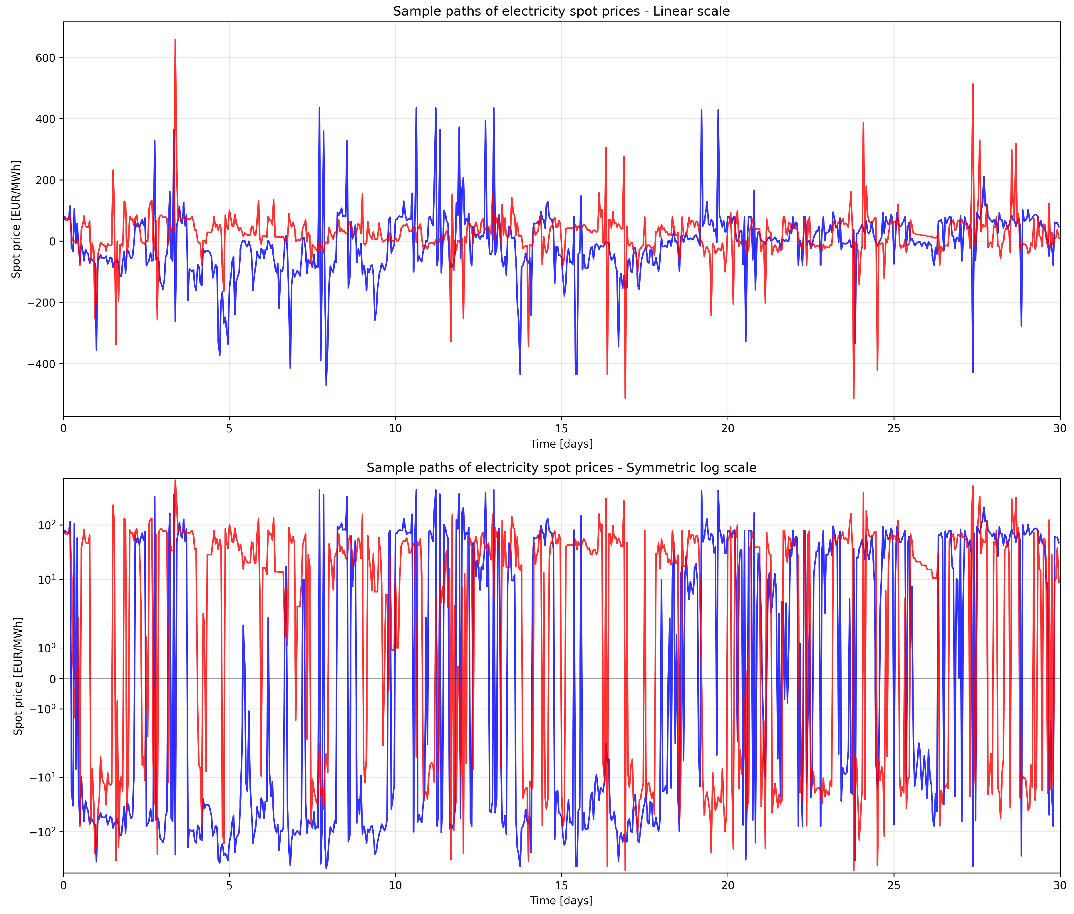
Figure 2.
Annual seasonality decomposition showing original vs deseasonalized prices (top), extracted annual pattern (middle), distribution comparison (bottom left), and monthly seasonal effects (bottom right).
Figure 2.
Annual seasonality decomposition showing original vs deseasonalized prices (top), extracted annual pattern (middle), distribution comparison (bottom left), and monthly seasonal effects (bottom right).
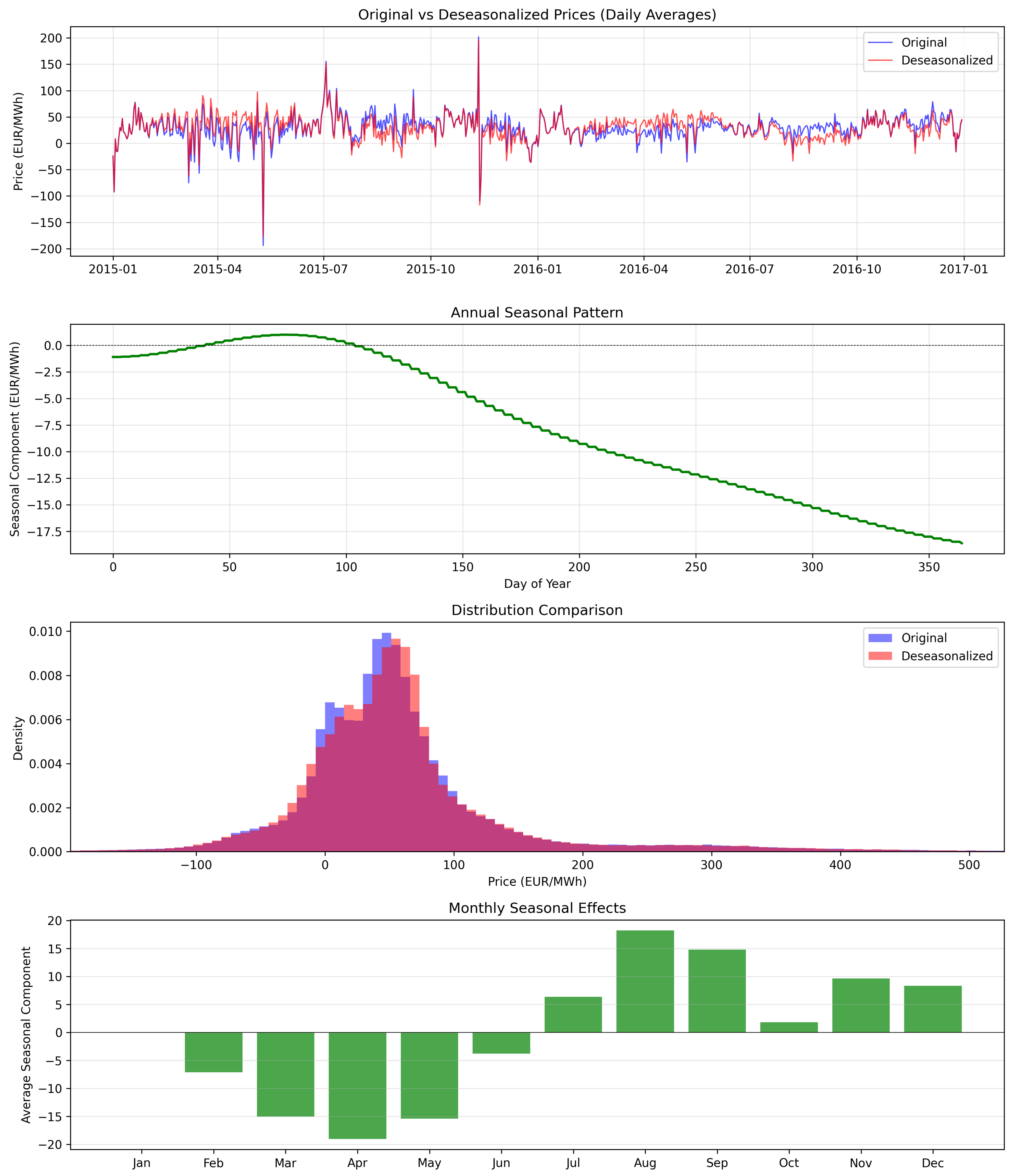
Figure 3.
Fourier decomposition results showing intraday pattern fit (R² = 0.943), weekly pattern fit (R² = 0.417), coefficient magnitudes, and decomposition summary statistics.
Figure 3.
Fourier decomposition results showing intraday pattern fit (R² = 0.943), weekly pattern fit (R² = 0.417), coefficient magnitudes, and decomposition summary statistics.
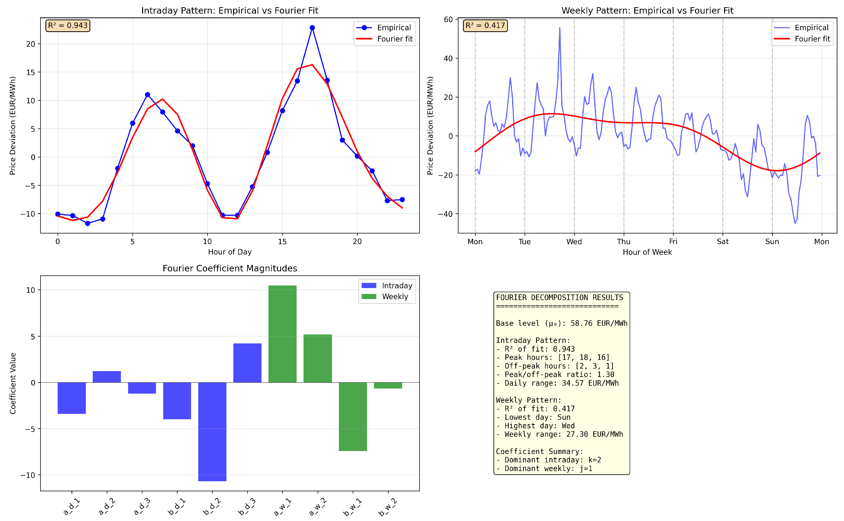
Figure 4.
Comprehensive analysis of log returns. Top left: histogram with fitted normal distribution showing heavy tails. Top right: QQ-plot revealing systematic deviations from normality. Middle: time series of log returns displaying volatility clustering. Bottom: comparison of statistics between log and simple returns, and autocorrelation function.
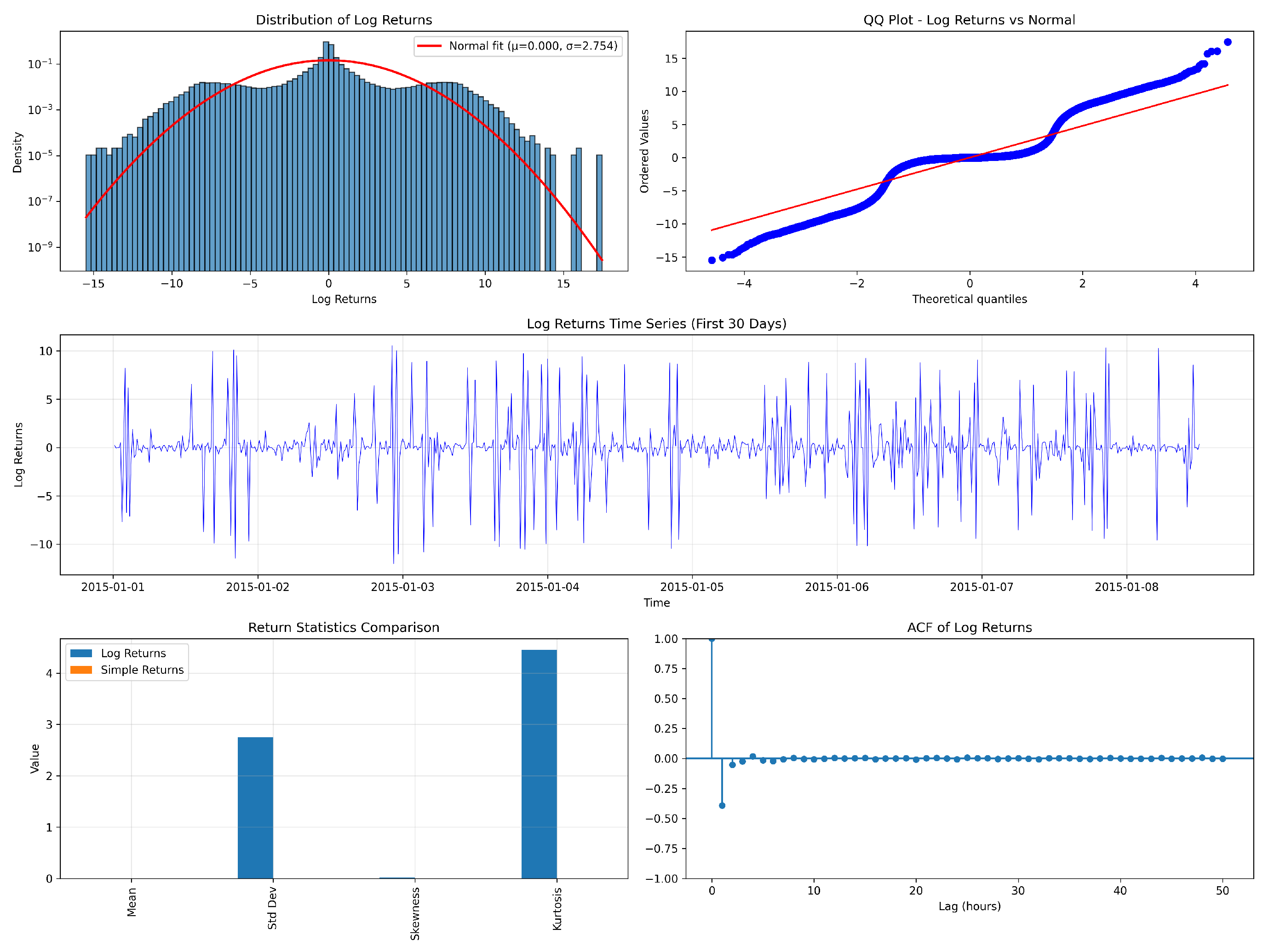
Figure 5.
Volatility clustering analysis. Left: ACF of squared log returns showing persistent autocorrelation indicative of volatility clustering. Right: Time-varying volatility computed using 7-day rolling windows, revealing distinct volatility regimes.
Figure 5.
Volatility clustering analysis. Left: ACF of squared log returns showing persistent autocorrelation indicative of volatility clustering. Right: Time-varying volatility computed using 7-day rolling windows, revealing distinct volatility regimes.
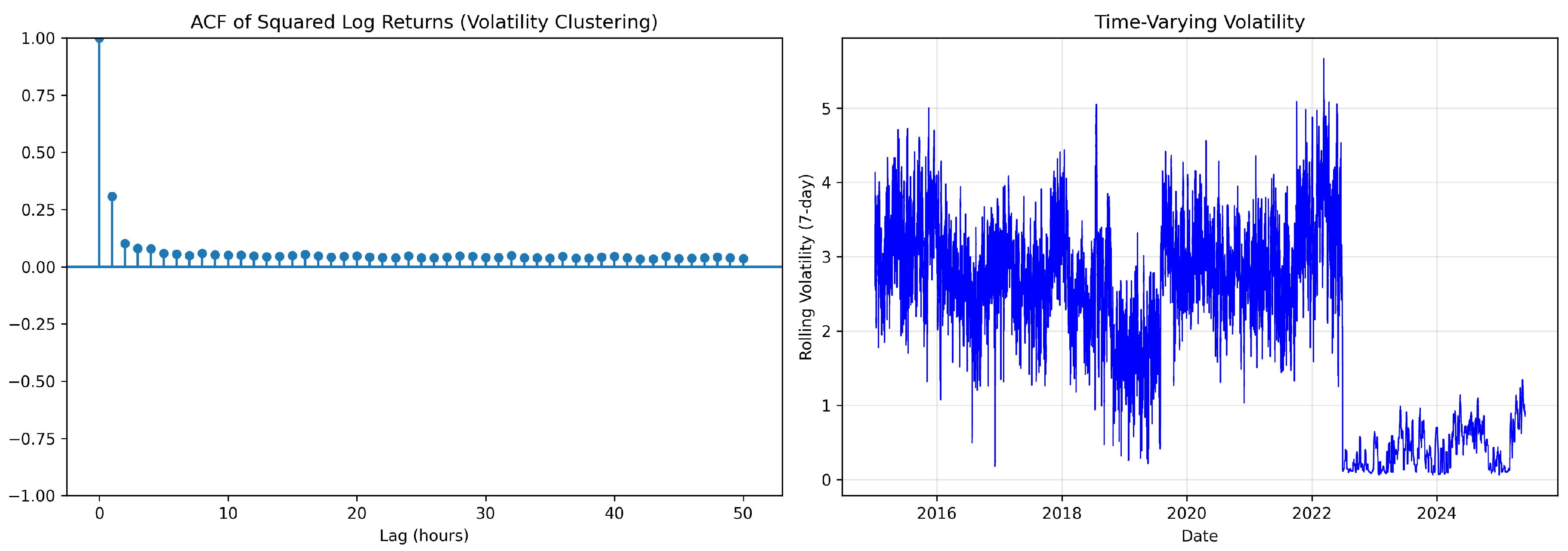
Figure 7.
Spectral analysis of electricity prices. Top left: Power spectrum on log-log scale showing power-law decay with embedded periodicities. Top right: Identified peak frequencies corresponding to daily and weekly cycles. Bottom left: Autocorrelation function confirming periodic structure. Bottom right: Welch’s periodogram highlighting daily and weekly frequencies.
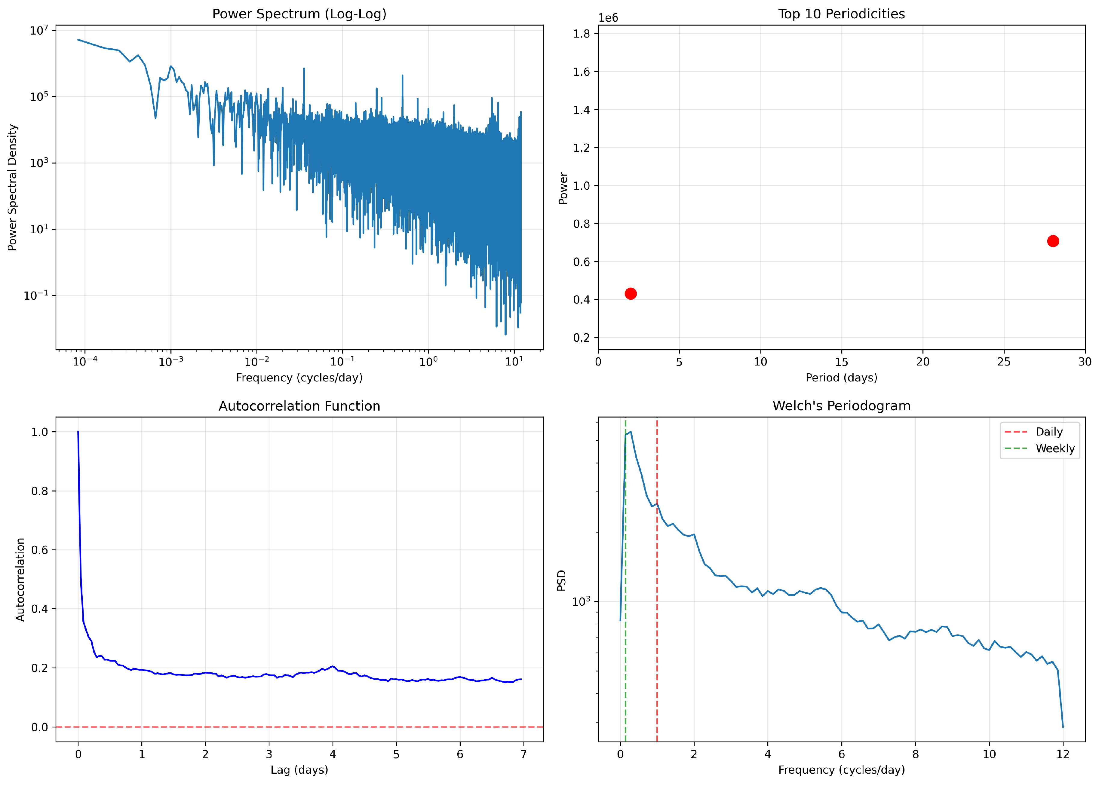
Figure 8.
STL decomposition with daily period. From top to bottom: original series, extracted trend showing medium-term evolution, 24-hour seasonal component displaying regular daily pattern (30 days shown), and residual component containing irregular variations and extreme events.
Figure 8.
STL decomposition with daily period. From top to bottom: original series, extracted trend showing medium-term evolution, 24-hour seasonal component displaying regular daily pattern (30 days shown), and residual component containing irregular variations and extreme events.
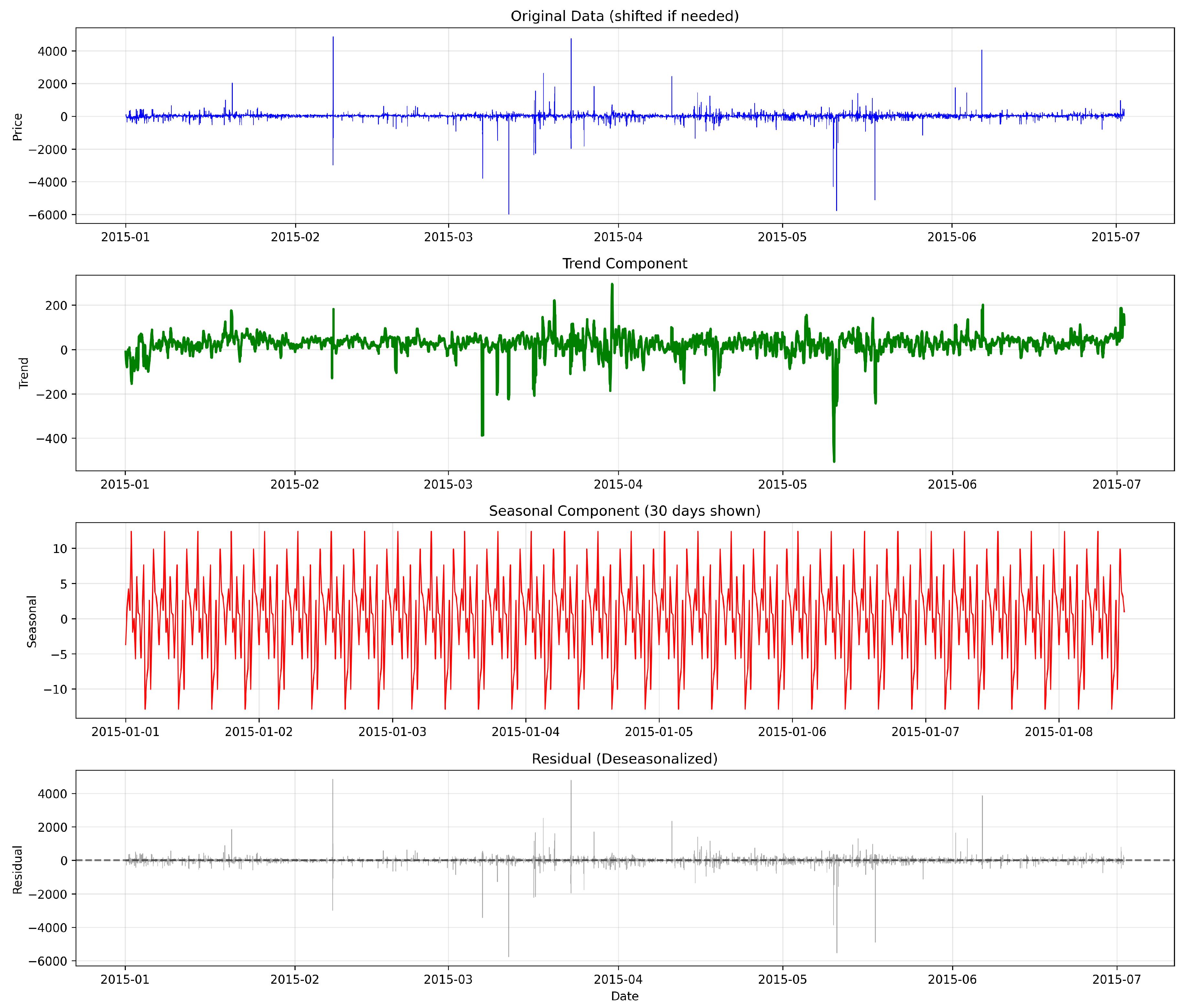
Figure 9.
Multi-scale seasonal patterns. Top row: intraday pattern showing morning and evening peaks, weekly pattern revealing weekend effects. Middle row: monthly seasonality and hour-day heatmap. Bottom row: negative price frequency by hour and extracted weekly seasonal component.
Figure 9.
Multi-scale seasonal patterns. Top row: intraday pattern showing morning and evening peaks, weekly pattern revealing weekend effects. Middle row: monthly seasonality and hour-day heatmap. Bottom row: negative price frequency by hour and extracted weekly seasonal component.
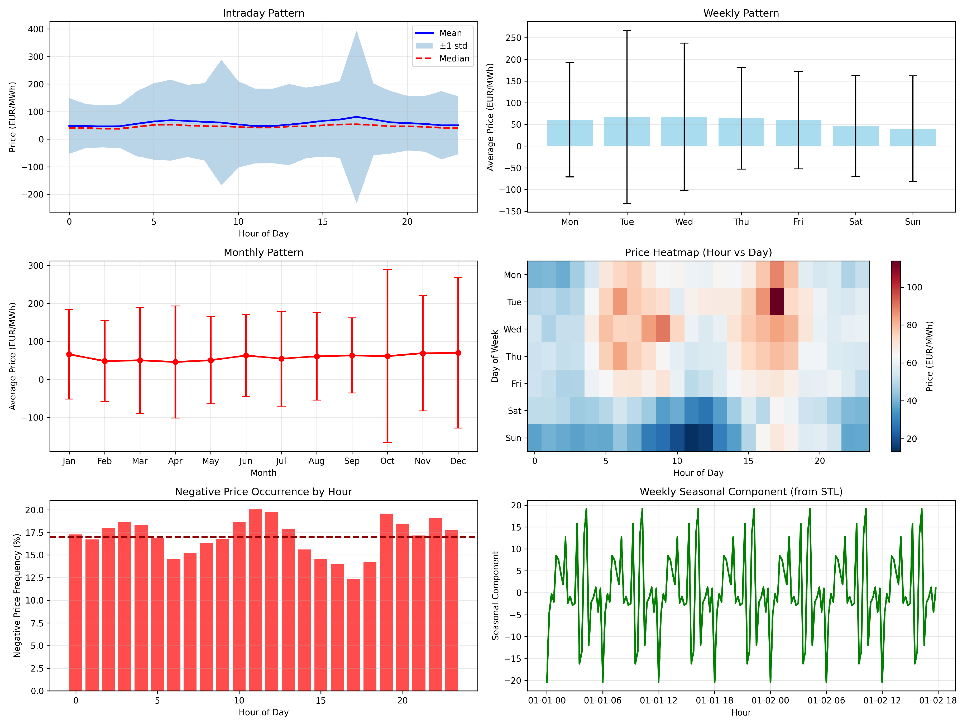
Figure 10.
Comprehensive spike analysis. Top: 90-day price series with identified positive (red) and negative (blue) spikes and rolling mean. Bottom left: spike magnitude distribution on log-log scale showing heavy tails. Bottom right: inter-arrival time distribution with fitted exponential model.
Figure 10.
Comprehensive spike analysis. Top: 90-day price series with identified positive (red) and negative (blue) spikes and rolling mean. Bottom left: spike magnitude distribution on log-log scale showing heavy tails. Bottom right: inter-arrival time distribution with fitted exponential model.
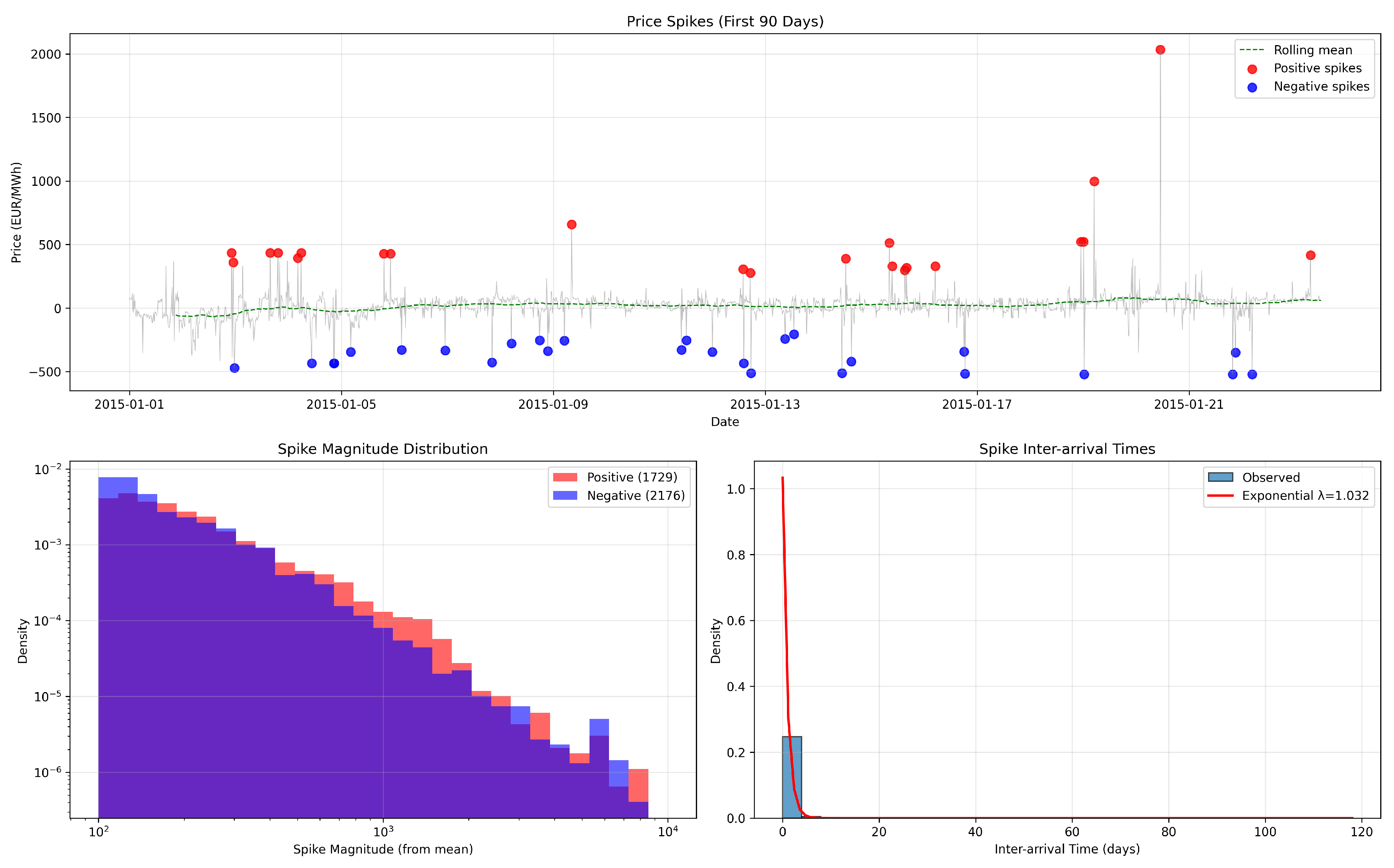
Figure 11.
Jump dynamics analysis using relative price changes. Top left: jump size distribution showing symmetric heavy tails for positive and negative jumps. Top right: inter-arrival times with exponential fit. Bottom left: distribution of daily jump counts compared to Poisson model. Bottom right: summary statistics revealing balanced positive/negative jump occurrences.
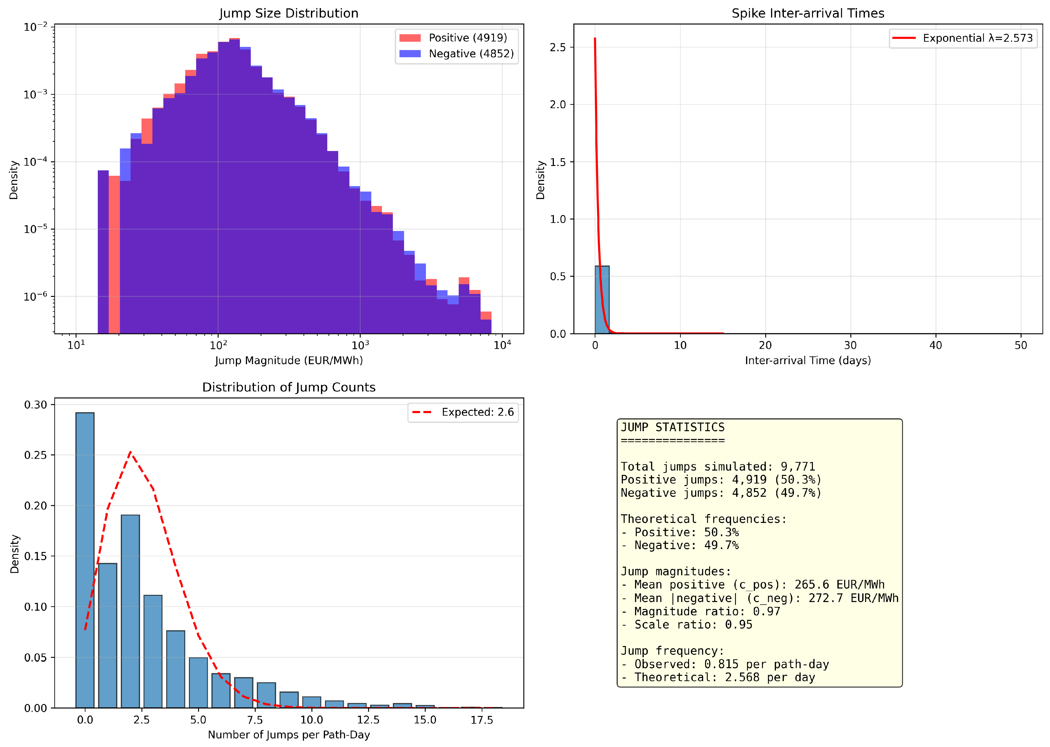
Figure 12.
Asymmetric tail analysis for electricity prices. Left: positive price tail distribution showing Pareto fit with empirical above threshold 271.9 EUR/MWh. Right: negative price tail distribution with heavier tail empirical above threshold 95.3 EUR/MWh, indicating more extreme negative price events.
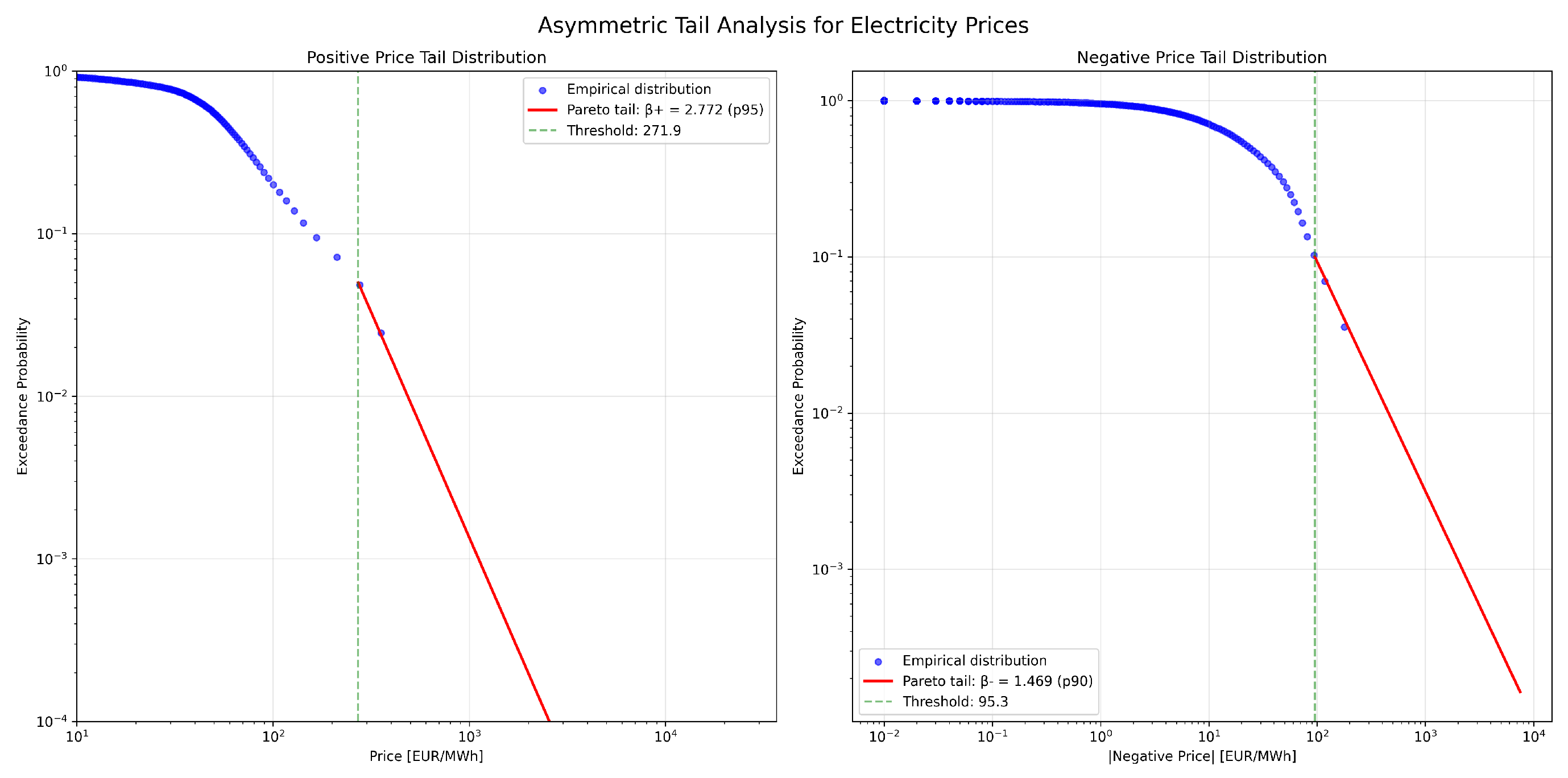
Figure 13.
Hill plots for tail index estimation showing stability regions (shaded green) for both positive and negative tails. The plots confirm the robustness of the tail index estimates.
Figure 13.
Hill plots for tail index estimation showing stability regions (shaded green) for both positive and negative tails. The plots confirm the robustness of the tail index estimates.
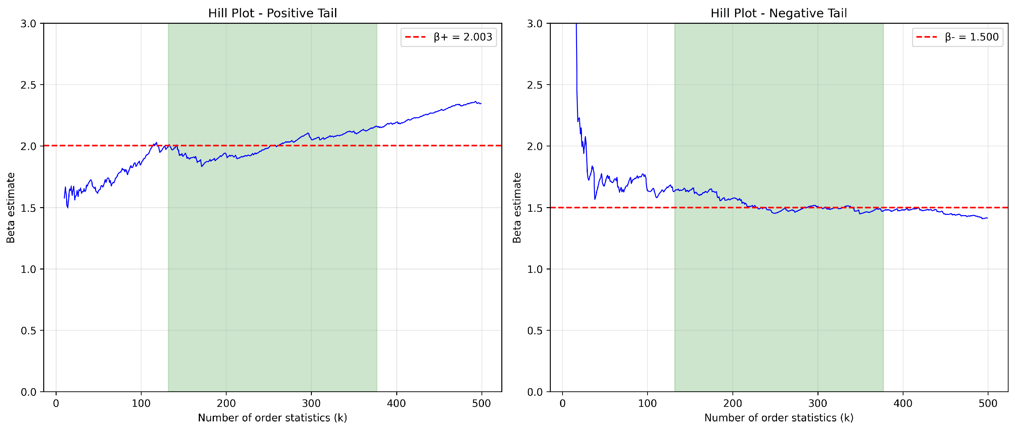
Figure 14.
Comprehensive trend analysis. Top row: raw prices with linear trend and monthly averages with trend. Middle row: yearly averages showing inter-annual variability and 365-day rolling mean revealing medium-term cycles. Bottom row: detrended prices and statistical summary of trend estimates.
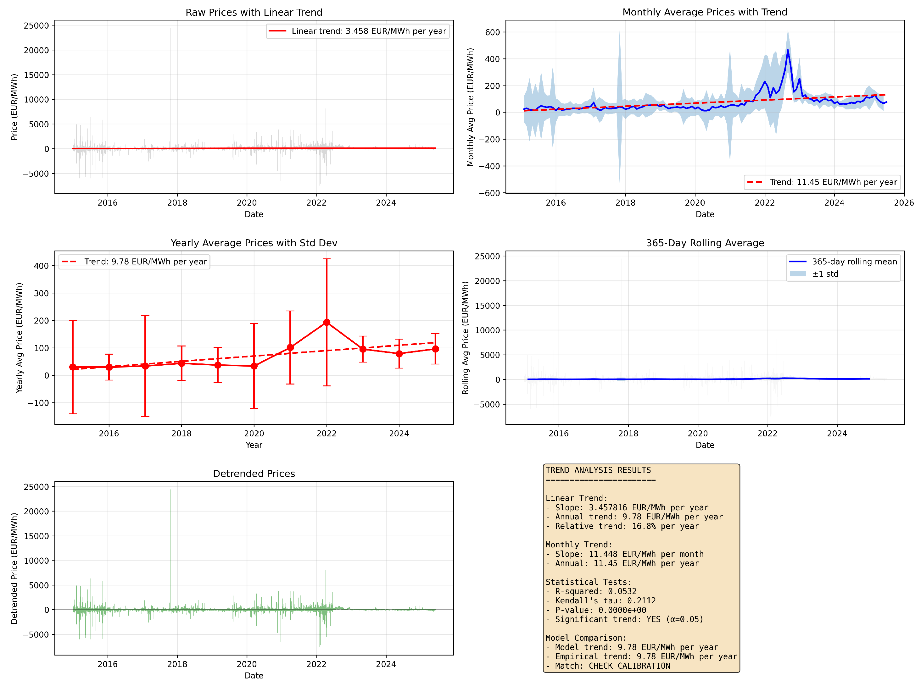
Figure 15.
Sample paths of simulated electricity spot prices over 30 days. The upper panel displays the full price range including extreme spikes up to 1,900 EUR/MWh and drops to -800 EUR/MWh. The lower panel uses a logarithmic scale revealing the regular price dynamics with visible daily seasonality and frequent negative price episodes.
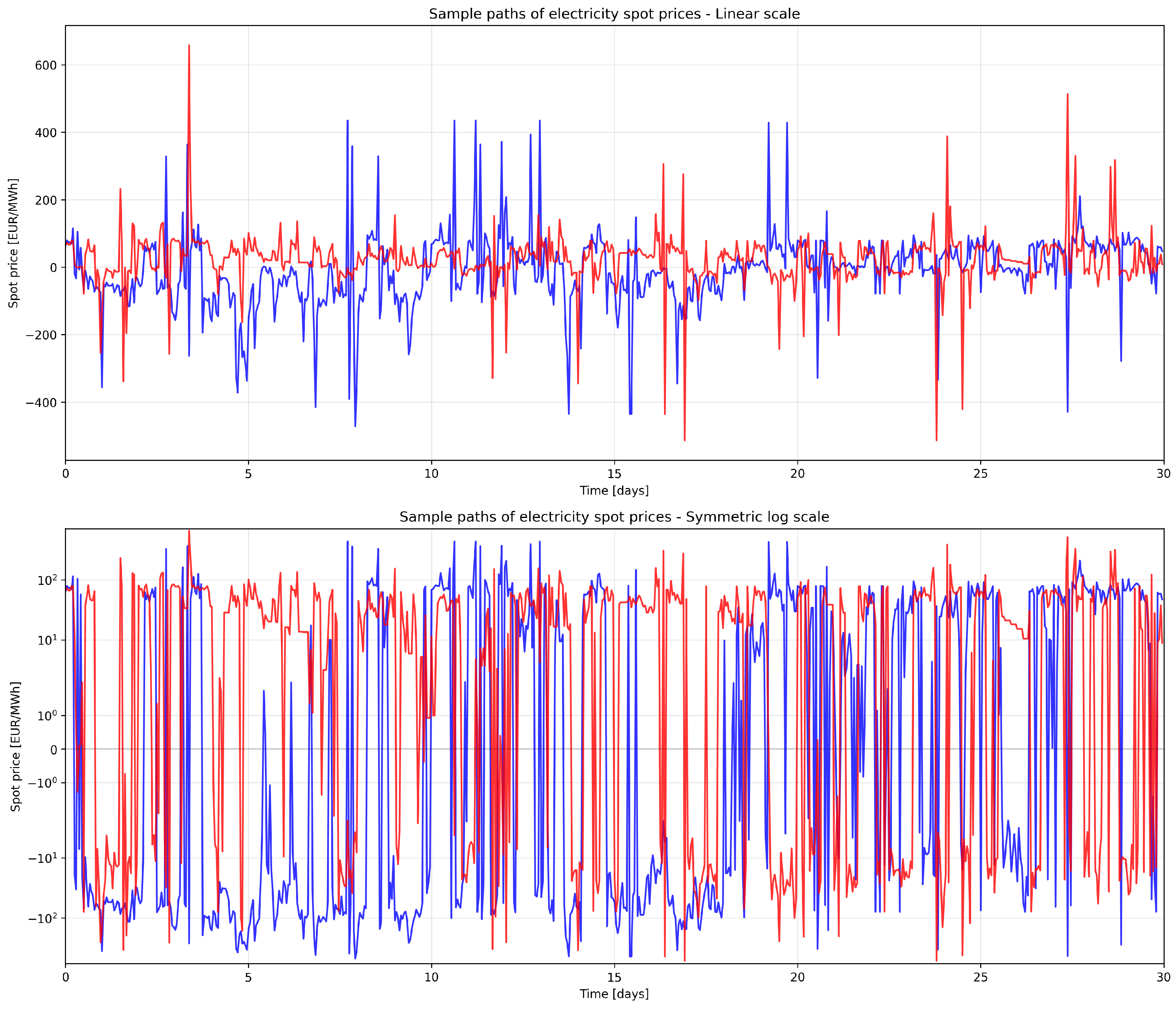
Figure 16.
Seasonal decomposition of simulated prices. Top: Average path across all simulations showing clear daily and weekly patterns. Second: Theoretical weekly seasonal pattern from Fourier coefficients showing weekend effects. Third: Linear trend component ( EUR/MWh per year). Bottom: Price distribution with key percentiles marked.
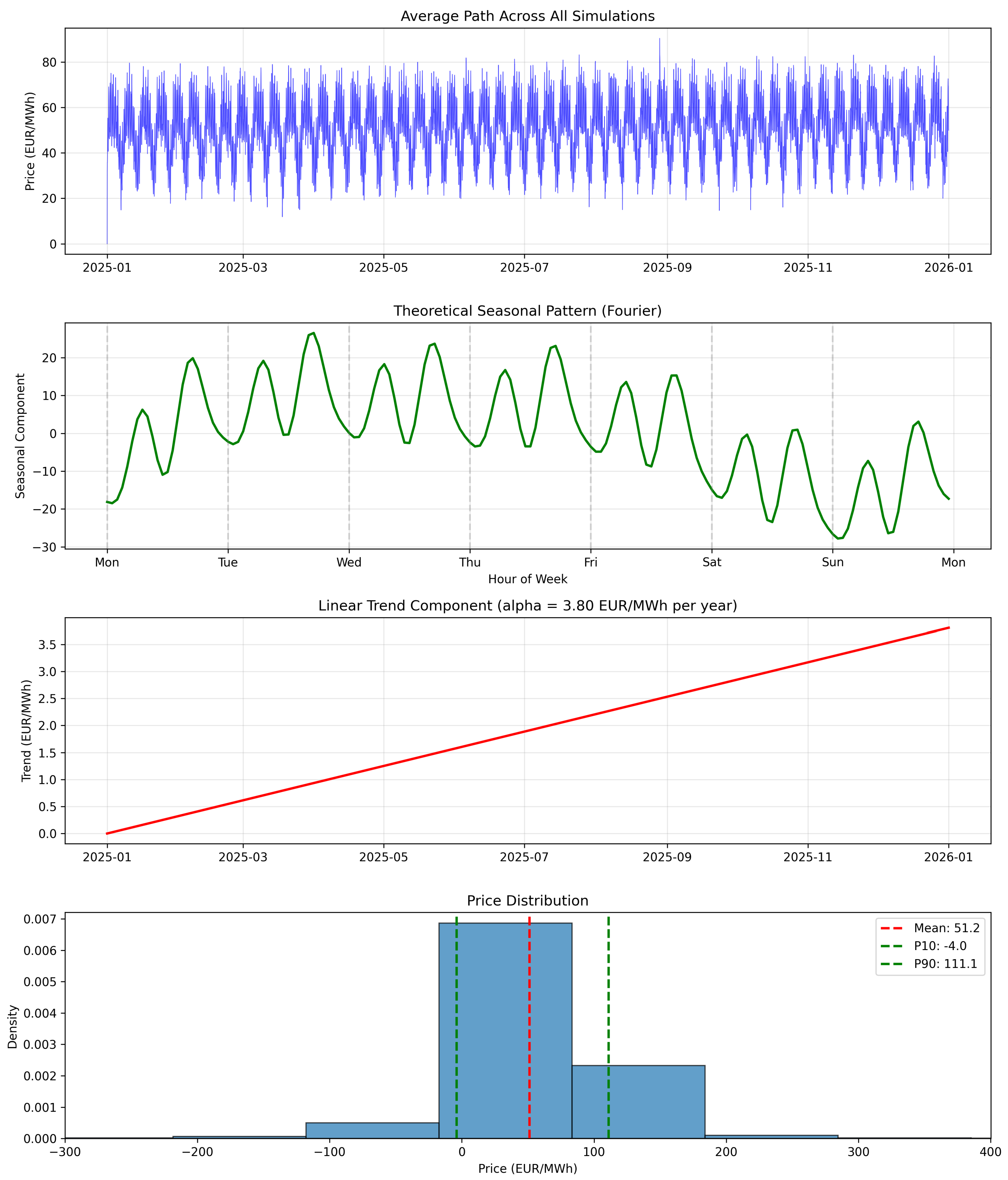
Figure 17.
Fourier decomposition analysis. Upper left: Comparison of theoretical and empirical intraday patterns showing excellent agreement with morning (8-9 AM) and evening (6-7 PM) peaks. Upper right: Weekly pattern capturing weekday-weekend dynamics. Lower left: Fourier coefficient magnitudes highlighting dominant components ( for intraday, for weekly). Lower right: Summary statistics.
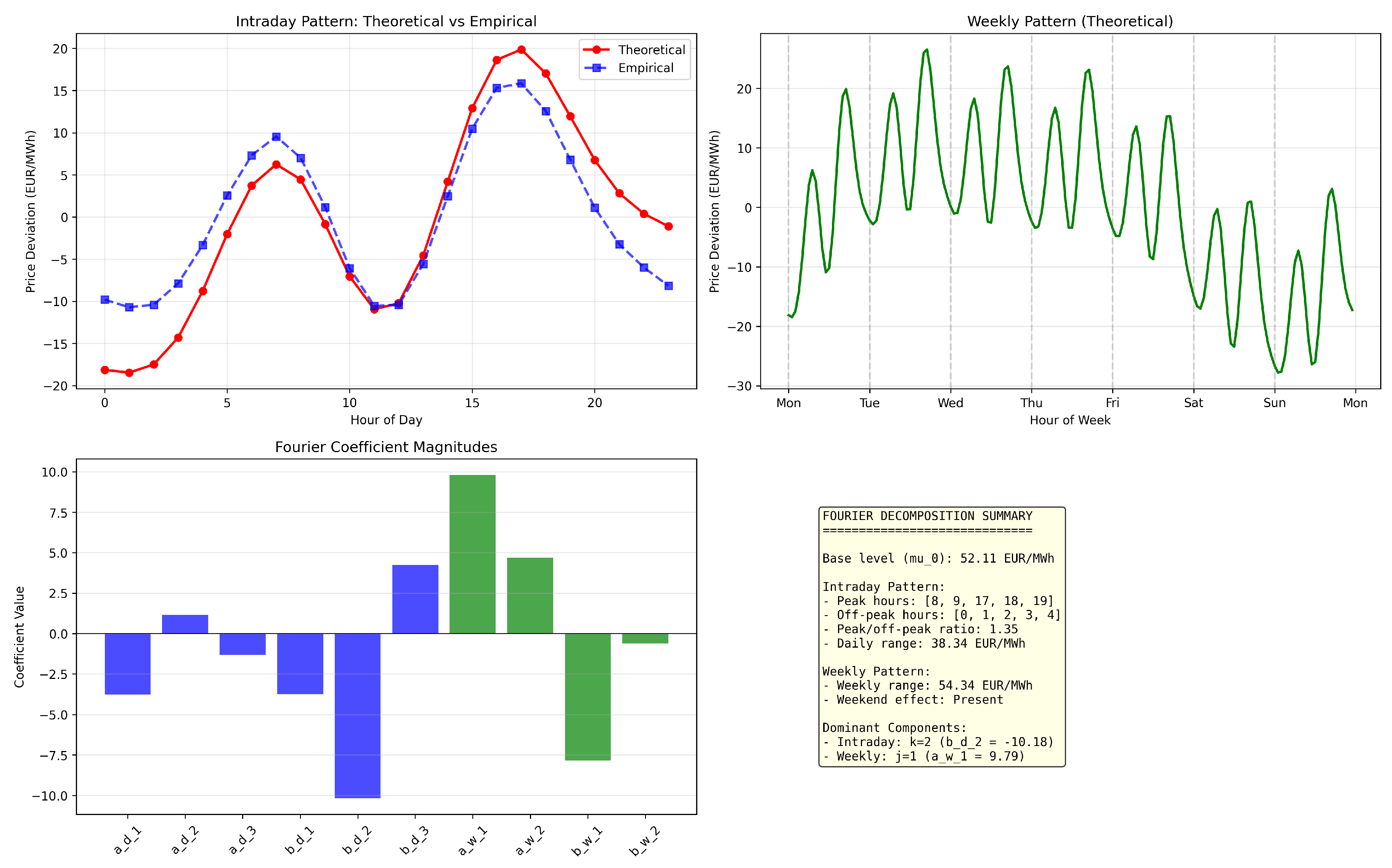
Figure 18.
Structural parameter validation. Upper left: ACF of deseasonalized prices showing empirical (blue) and theoretical (red dashed) exponential decay with h. Upper right: Jump identification on a sample path. Lower left: ACF of squared returns confirming volatility clustering. Lower right: Comparison of theoretical and empirical structural metrics.
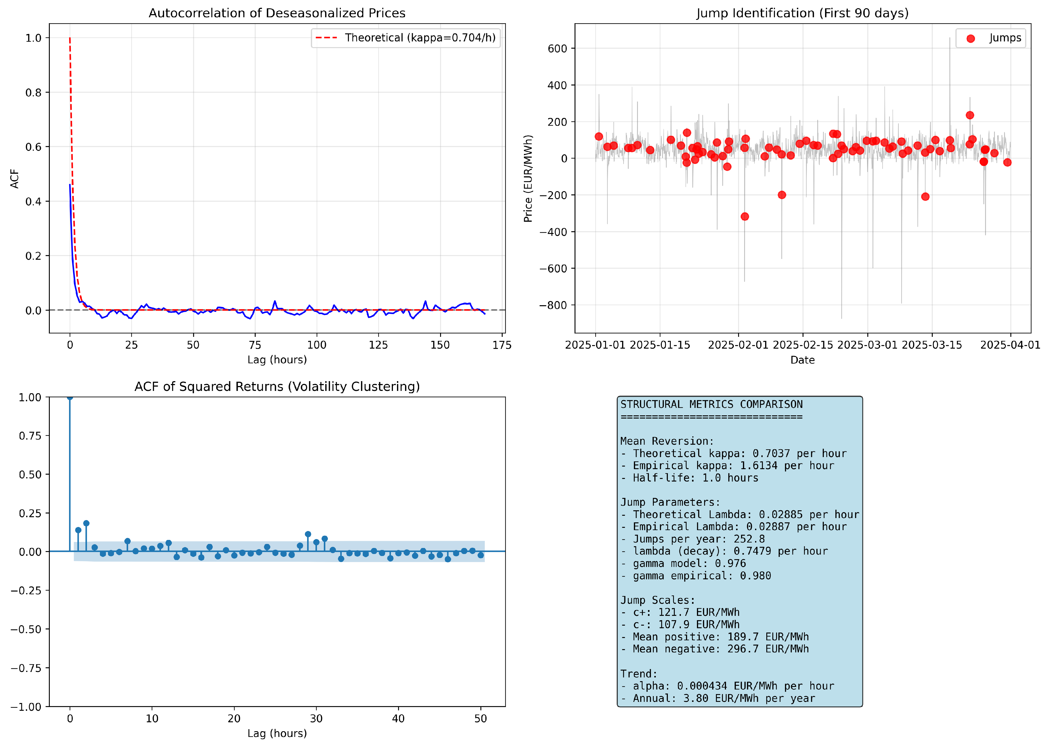
Figure 19.
Log returns analysis revealing heavy-tailed behavior. Left: Distribution on log scale showing extreme deviations from normality. Upper right: QQ-plot confirming systematic departures in both tails. Middle: Time series of log returns showing volatility clustering. Bottom: Return statistics and ACF indicating near-zero linear autocorrelation but significant nonlinear dependence.
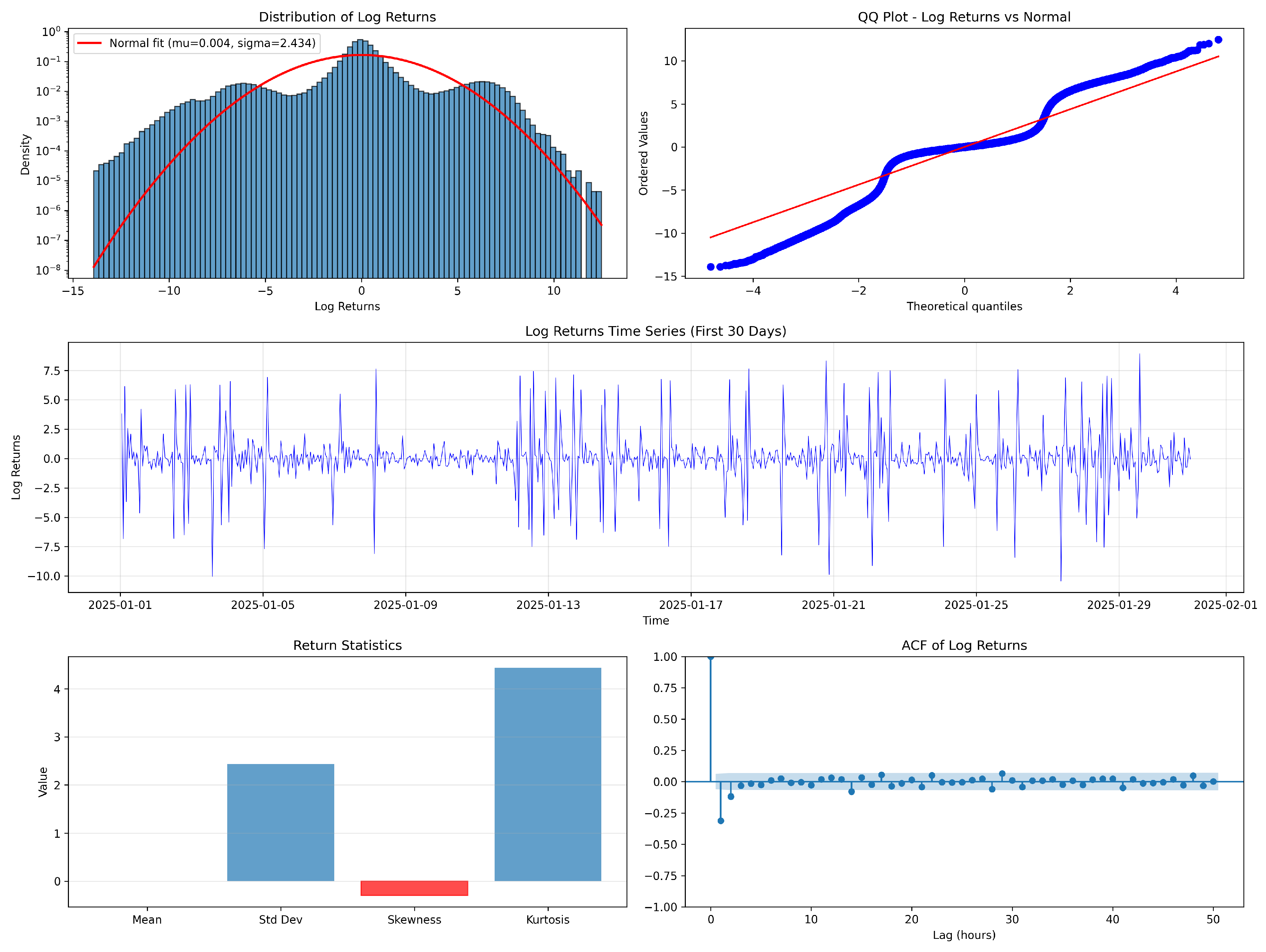
Figure 20.
Asymmetric tail analysis on log-log scale. Left: Positive price tail with Pareto fit above threshold 114.5 EUR/MWh. Right: Negative price tail with heavier Pareto fit above threshold 77.1 EUR/MWh. The asymmetry reflects greater probability of extreme negative prices during oversupply conditions.
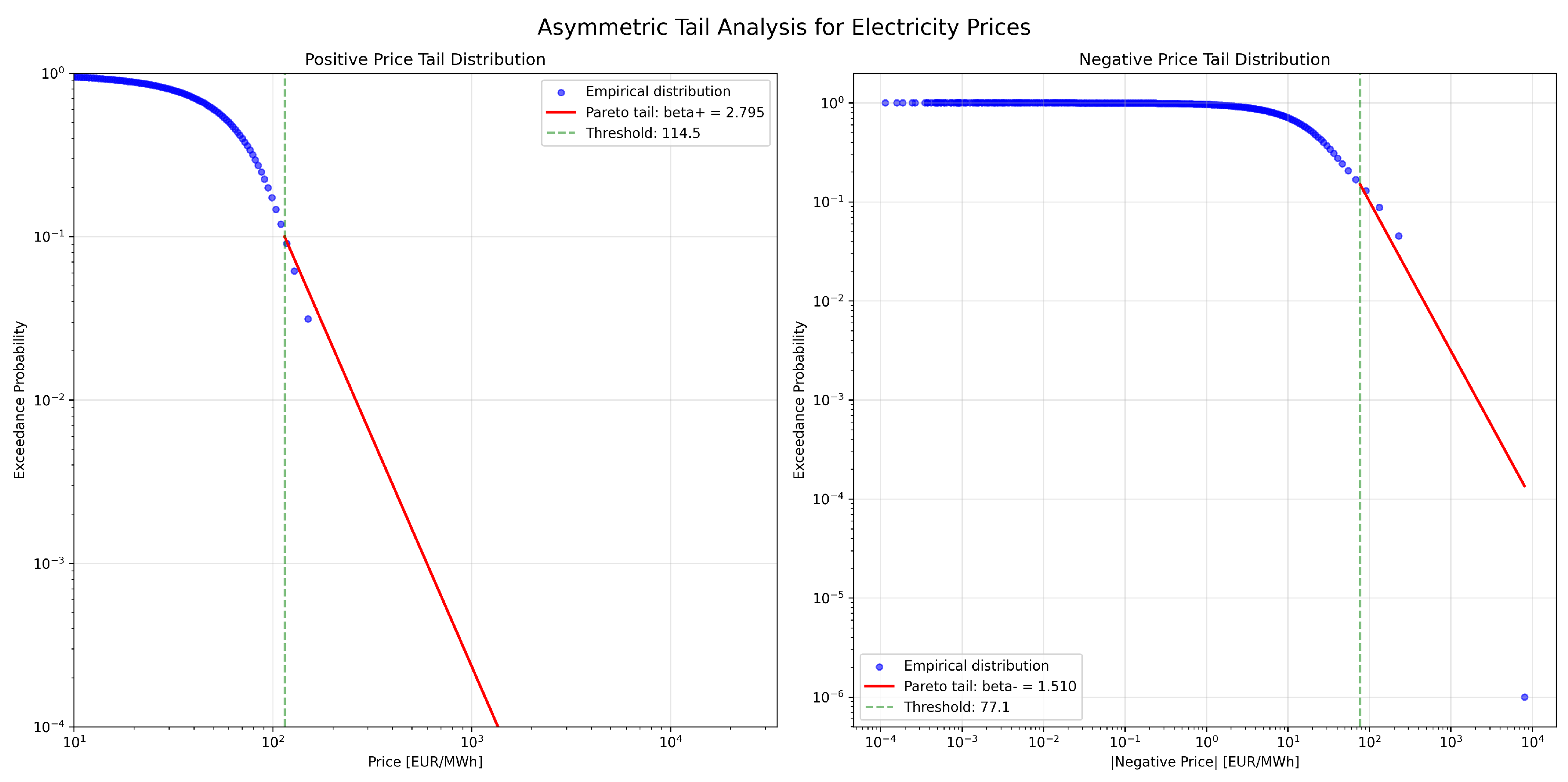
Figure 21.
Comprehensive jump analysis. Upper left: Jump size distributions on log-log scale showing power-law tails for both positive (127,746) and negative (125,131) jumps. Upper right: Exponential inter-arrival times with theoretical fit. Lower left: Daily jump count distribution compared to Poisson model. Lower right: Summary statistics confirming balanced frequency but asymmetric magnitudes.
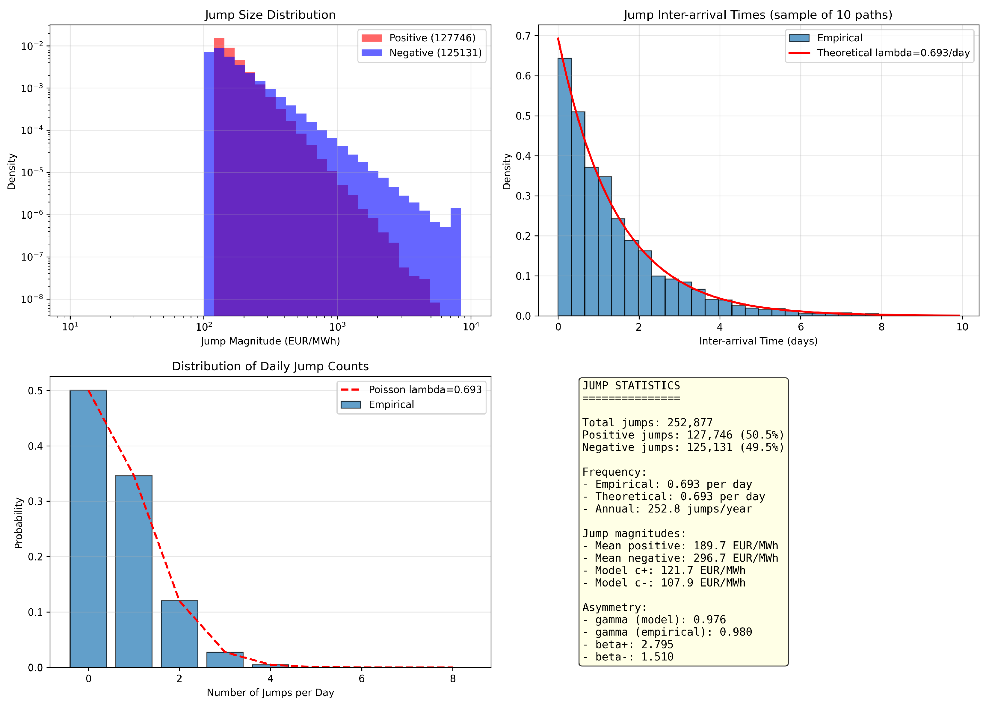
Figure 22.
Multi-scale seasonal patterns. Upper panels: Intraday mean prices showing double peaks and weekly averages revealing weekend effects. Middle panels: Monthly trend including linear growth and hour-day price heatmap. Lower panels: Negative price frequency by hour showing bimodal pattern (night and midday peaks) characteristic of renewable-dominated systems.
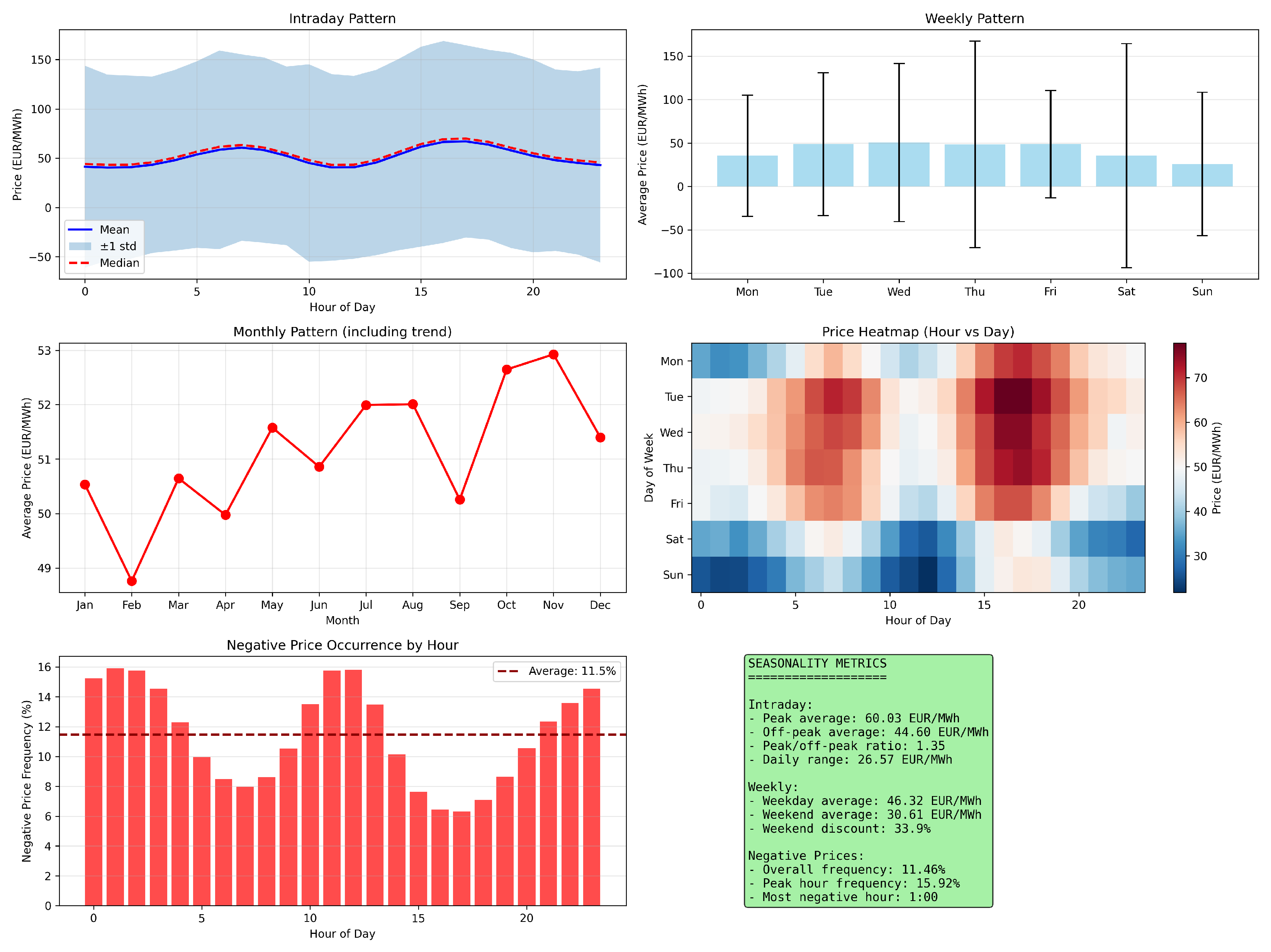
Figure 23.
Volatility dynamics. Upper left: 7-day rolling volatility showing time-varying risk. Upper right: ACF of squared returns with significant persistence confirming volatility clustering. Lower left: Distribution of path volatilities. Lower right: Summary metrics including Ljung-Box test rejecting independence (p-value < 0.0001).
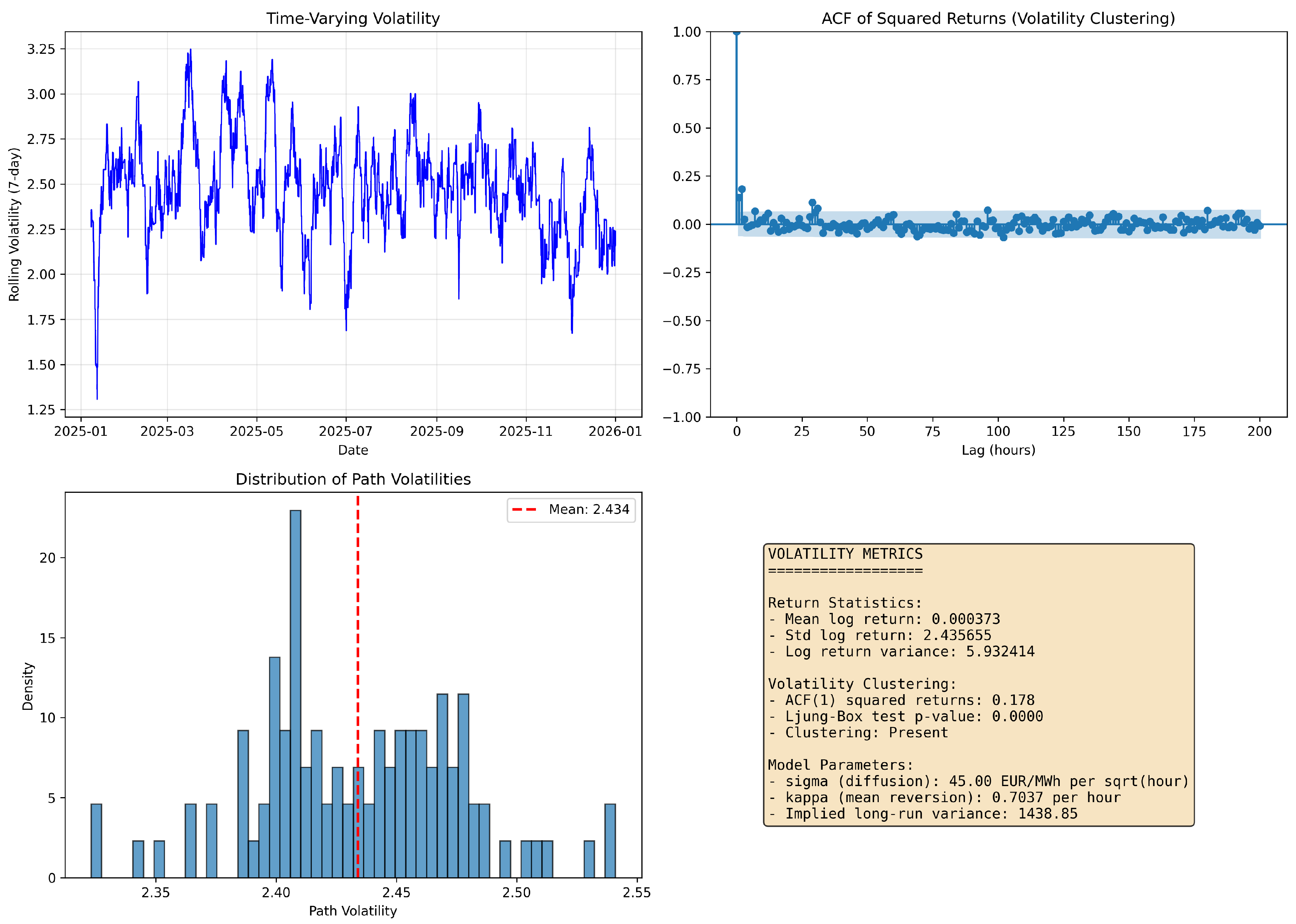
Table 1.
Key Statistics of German Electricity Spot Prices (2015–2025)
| Statistic | Value |
|---|---|
| Mean price | 58.16 EUR/MWh |
| Standard deviation | 142.12 EUR/MWh |
| Coefficient of variation | 2.444 |
| Skewness | 18.73 |
| Excess kurtosis | 1847.2 |
| Minimum pricea | −7507.00 EUR/MWh |
| Maximum pricea | 24 455.05 EUR/MWh |
| 10th percentile | −16.91 EUR/MWh |
| 90th percentile | 139.68 EUR/MWh |
| Negative price frequency (15-min)b | 16.99% |
| Negative price frequency (hourly avg)c | 8.47% |
| Days with any negative hour | 22.8% |
a Values may reflect pre-harmonization caps. b Share of quarter-hours. c Share of hours whose mean of four quarter-hours is negative.
Table 2.
Estimated Fourier Coefficients
| Parameter | Value | Parameter | Value |
|---|---|---|---|
| 58.76 | 10.49 | ||
| -3.40 | -7.43 | ||
| -3.98 | 5.19 | ||
| 1.24 | -0.64 | ||
| -10.67 | |||
| -1.21 | |||
| 4.22 |
Disclaimer/Publisher’s Note: The statements, opinions and data contained in all publications are solely those of the individual author(s) and contributor(s) and not of MDPI and/or the editor(s). MDPI and/or the editor(s) disclaim responsibility for any injury to people or property resulting from any ideas, methods, instructions or products referred to in the content. |
© 2025 by the authors. Licensee MDPI, Basel, Switzerland. This article is an open access article distributed under the terms and conditions of the Creative Commons Attribution (CC BY) license (http://creativecommons.org/licenses/by/4.0/).
Copyright: This open access article is published under a Creative Commons CC BY 4.0 license, which permit the free download, distribution, and reuse, provided that the author and preprint are cited in any reuse.


