Submitted:
30 January 2026
Posted:
02 February 2026
You are already at the latest version
Abstract
The motion prediction of semi-submersible platforms is of significant importance for improving operational efficiency, ensuring platform safety, and providing early warning information for potential risks. Traditional prediction methods, such as those based on hydrodynamic simulations combined with Kalman filters, often face limitations due to their reliance on precise hydrodynamic parameters, which are difficult to obtain in practice. More recently, data-driven approaches, particularly deep learning models like Long Short-Term Memory (LSTM) networks, have shown promise in predicting complex motions. However, these methods often treat the prediction process as a “black box,” leading to issues such as lack of generalization ability, overfitting, and an inability to quantify the uncertainty of prediction results. To address these challenges, this paper proposes a novel motion prediction method for semi-submersible platforms based on a Bayesian neural network (BNN). The BNN incorporates Bayesian inference to effectively integrate prior knowledge and measured data, thereby quantifying uncertainties and improving prediction accuracy. The method is validated using field-measured motion data from a semi-submersible platform in the South China Sea. Compared with LSTM networks, the BNN demonstrates superior anti-noise performance and prediction accuracy, achieving an accuracy rate of up to 91.5%. Moreover, over 92% of the true values are captured within the 95% confidence interval of the prediction results. This study highlights the potential of BNNs for real-time motion prediction of offshore platforms, providing valuable support for early warning systems and operational decision-making.
Keywords:
semi-submersible platform
; motion prediction
; Bayesian neural network
; deep learning
; uncertainty quantification
; field monitoring
1. Introduction
Semi-submersible platforms, as typical offshore floating structures, have been extensively utilized in deepwater oil and gas exploration due to their large deck operation areas, excellent stability, and significant adaptability to varying water depths (Chen, 2011, Sharma et al., 2010, Chen et al., 2017, Wang et al., 2010). Under the influence of extreme marine environmental loads, these platforms may experience large-amplitude six-degree-of-freedom (6 DOF) motions, which directly impact the safety of drilling, maintenance, and other production operations. Accurate real-time prediction of these motions can provide effective early warning information to ensure the safety and efficiency of platform operations.
The prediction of the motions of semi-submersible platforms has primarily focused on two approaches: hydrodynamic simulation combined with Kalman filtering and data-driven methods. As early as the 1980s, scholars began analyzing and predicting the motions of marine equipment based on hydrodynamic simulation results, with Triantafyllou (2023) using the Kalman filter to predict ship motions. However, the accuracy of the Kalman filter is closely related to hydrodynamic parameters such as added mass and damping coefficients, which limits its practical application. More recently, Naaijen et al. (2009) predicted the motions of semi-submersible platforms by forecasting wave parameters and combining them with hydrodynamic simulations, achieving high-precision results. Nevertheless, these results are highly dependent on the accuracy of the response amplitude operator (RAO). Research by Faltinsen et al. (1993) indicated that the sway, surge, and yaw motions of floating platforms mainly depend on the restoring force provided by the mooring system. Therefore, comprehensively and accurately predicting the motion behavior of offshore platforms remains challenging when relying solely on marine environment and hydrodynamic simulation.
In recent years, machine learning, especially deep learning, has rapidly developed for fitting complex mapping analyses. Khan et al. (2005) used a genetic algorithm and singular value decomposition to train a three-layer fully connected neural network to predict rolling motions. The introduction of Long Short-Term Memory (LSTM) networks in 1997 (Hochreiter et al., 1997) has led to their widespread application in time-series prediction. Research by Duan et al. (2019) demonstrated that LSTM networks have good accuracy in predicting ship motions. Deng et al. (2021) built prediction models for roll, pitch, and heave motions of semi-submersible platforms using fully connected neural networks and LSTM, verifying their accuracy with experimental data. Silva et al. (2022) trained LSTM networks using data from computational fluid dynamics (CFD) simulations to predict ship motions under extreme conditions.
Despite the extensive use of LSTM-based deep learning methods for predicting motions of marine structures, these methods often face challenges such as lack of model generalization ability, overfitting with increasing layers, and difficulty in quantifying uncertainties. Traditional neural networks automatically set weight coefficients during training without considering prior data information, leading to suboptimal solutions. Moreover, these models cannot clearly present the confidence intervals of prediction results, which are crucial for practical decision-making.
To address these limitations, this study proposes a novel motion prediction method for semi-submersible platforms using a Bayesian neural network (BNN). The BNN incorporates Bayesian inference to effectively integrate prior knowledge and measured data, thereby quantifying uncertainties and optimizing the weight parameters of the neural network. The method is validated using field-measured motion data from a semi-submersible platform in the South China Sea, demonstrating its potential for practical applications in offshore engineering.
This paper is organized as follows: Section 2 introduces the neural network solution method of the Bayesian principle, and gives the accuracy of this method in solving nonlinear problems. Section 3 introduces the motion prediction method and prediction results of a semi-submersible platform in the South China Sea. The prediction results are further discussed in Section 4. The conclusion of this paper is presented in Section 5.
2. Bayesian Parameter Optimization Neural Network Model
2.1. Bayesian Theories in Neural Networks
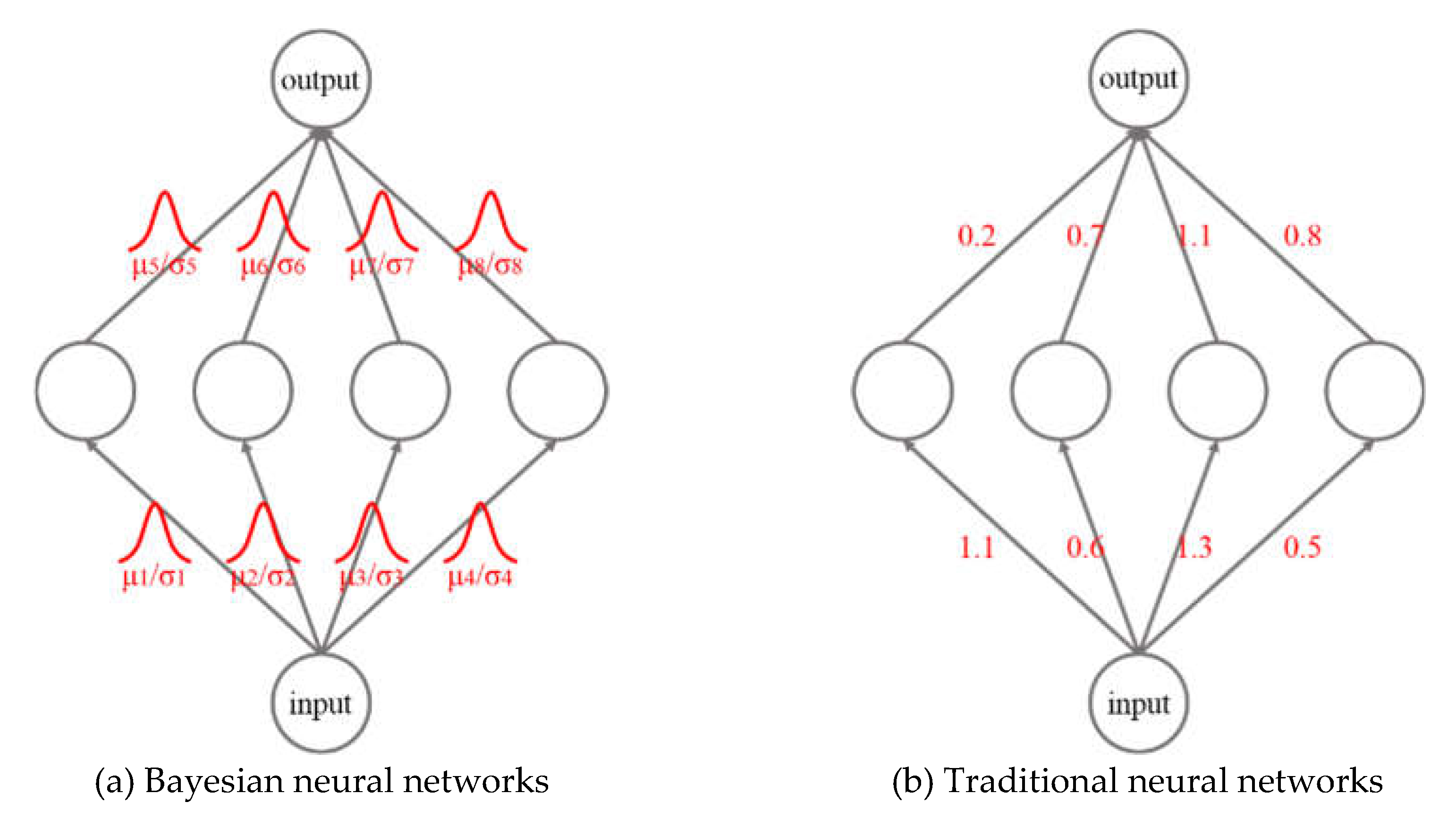
The process of building a relationship of neural network mainly depends on input data. But the noise of input data will greatly affect the accuracy of the neural networks. Unlike the traditional neural network in which the weight parameters are directly obtained from model training, this paper uses Bayesian inference to solve the distribution of the weight matrix w, where D = {(x,y)} is the input and output of the training model. Therefore, the training process of a traditional neural network is transformed into the process of solving the posterior distribution of w, which is shown in formula (1).
Then the output value of the new input data point is predicted based on the distribution of w. The posterior distribution of the predicted value is shown in formula (2). Fig. 1 shows the difference between this method and the traditional neural network in the prediction process.
where is the prior distribution of the weight matrix, which is directly given based on experience, is the posterior distribution of the weight matrix, which is mainly used for data prediction based on the weight matrix, can also be written as, also known as evidence [14], is the posterior distribution of the weight matrix, which is mainly trained by the input data. According to formula (1), if the prior distribution of w is known, the learning process of the neural network will become a process of solving the maximum posterior estimate, which is.
However, in the case of the distribution law is unknown, in theory, infinite sets of operations are required to solve the maximum posterior estimation. When the neuron is a hidden layer, the posterior distribution of w is directly calculated by the gradient descent method. It is necessary to multiply the weight values of different points on the distribution function by the gradient of the output layer, which is huge for the neural network. Therefore, this paper establishes the variational form of the posterior distribution based on the variational estimation method, and finally converts the solution of the distribution into the process of solving its mean and variance.
Figure 1.
Traditional neural networks and Bayesian neural networks.
2.2. Variational Estimation
The main idea of variational estimation (Blei et al., 2017, Zhang et al., 2018) is to use a distribution controlled by a group of parameters θ to approach the real posterior, so that the problem of solving the posterior distribution is transformed into solving the optimal parameters θ. This process can be achieved by minimizing the KL divergence of two distributions (Kullback et al., 1951).
The form of the objective function is:
Among them, the first term is the KL divergence of the variational posterior and the prior, which describes the fit degree of the weight and the prior. The value of the second item depends on the training data and describes the fitting degree of the sample. The form of the objective function obtained by further defining KL divergence is:
According to the Monte Carlo approximation and the definition of data set D given in the literature [18], formula (5) can be converted into:
where wi is the weight of the ith data.
2.3. Network Weight Solving Procedure
According to the research of Blundell et al. [19], it can be assumed that the weight w is the combination of multiple normal distributions to solve the minimum value of formula (6). The weight expression is shown in formula (7):
where, then. To ensure that the value range of the parameter θ can contain the real number axis, and can effectively avoid the gradient vanishing when facing the complex network, so that the parameter, where ρ represents the given standard deviation. Therefore, parameter.
Therefore, it is easy to calculate and in formula (6) after sampling w. Because of, in formula (6) can be equivalent to. In practical applications, the standard deviation is determined according to the uncertainty of the measured data, and the current predicted value is taken as the mean value to determine a normal distribution. can be determined by sampling in the normal distribution.
If, then,
The process of solving network weights is as follows:
(1) Sample from to get w,
(2) It is assumed that the prior distribution of w is ,
(3) Calculate ,
(4) Determine by artificially given standard deviation and calculated,
(5) Repeat the above process to update parameters ,.
Note that the term of the gradients for the mean and standard deviation are shared and are exactly the gradients found by the usual backpropagation algrorithm on a neural network. In addition, the idea of Relu is fully used for reference to effectively avoid the problem of gradient vanishing in the process of solving w.
To sum up, the Bayesian neural network (BNN) achieves a good training results because it takes into account the prior information of the weight and uses the form of Relu activation function to equivalent the weight in the training process, taking into account the problem of gradient vanishing. In addition, because the predicted value of the BNN is the average of multiple predictions based on the network weight distribution, it effectively avoids the outliers in the prediction results.
2.4. An Example of the BNN Verification: Lorenz Dynamic System Considering the Influence of Noise
Lorentz equation is a typical equations for simulating atmospheric convection, and its expression is shown in formula (10). Lorentz equations, as a typical nonlinear equations, can be used to test the fitting effect of the BNN on nonlinear problems.
Among them, σ is the Prandt constant, r is the normalized Rayleigh number, and b is related to the geometric shape. In order to conduct relevant simulation research, σ takes 10, r as 28, and b as 8/3 to obtain the three-dimensional view of the Lorentz attractor as shown in Fig. 2.
To verify BNN's ability to resist the influence of noise, the coordinate information of the x-axis and y-axis of the Lorentz attractor is used as input, and the coordinate information of the z-axis is added to the noise data with a signal-to-noise ratio (SNR) of 10 as output. The SNR is defined as follows. If the noise in the signal s(n) is v(n), the SNR expression of the signal in the time domain is shown in formula (11):
Take 70% of the 30000 sets of data samples as training, 10% as validation, and 20% as testing. The author believes that the anti-noise ability mainly refers to the ability to find the original data in the noisy data, so the anti-noise ability of the BNN is evaluated by comparing the predicted results of the model with the original data without noise.
Through the training of the BNN, the comparison between the real test set data without noise and the predicted data is shown in Fig. 3, and the 95% confidence interval is given in Fig. 3. According to the prediction results, the BNN prediction results are good. And the original data points are basically included in the 95% confidence interval. It fully reflects the ability of the BNN to predict noisy data.
In addition, the LSTM neural network is trained by using the same data set division method as the BNN and the data without noise. Compare the prediction results of the LSTM and the BNN with the test set data without noise, the correlation comparison chart as shown in Fig. 4.
For comprehensive comparisons of prediction errors, root mean square error (RMSE) and R2 are defined as follows,
where 、 and represent the real data, prediction results and mean value of real data respectively.
The values of (RMSE) and R2 between the predicted values of the LSTM and the BNN and the test data without noise are given in Table 1.
The comparison shows that the prediction accuracy of the BNN model trained with noisy data is better than that of the LSTM model trained with noise-free data. It shows that the BNN can effectively overcome noise interference as well as have better accuracy than LSTM's prediction results when predicting raw data without noise. The feasibility, accuracy, and resistance to noise of the BNN method are verified.
3. Construction of Motion Prediction Model for Semi-Submersible Platform
3.1. Prototype Monitoring System of a Semi-Submersible Platform
Based on monitoring data from a semi-submersible platform, in this paper the motion prediction research of the hull of the platform is carried out. The sensor arrangement of the monitoring system is shown in Fig. 5 (Li et al., 2022).
3.2. Selection of Monitoring Data Set
1-second-interval motion data of 6 DOF of platform are used. The data are collected for 30 days, from January 1, 2014 to January 30, 2014, and included 43200 sets, as shown in Fig. 6.
At the same time, the frequency-domain characteristic diagram of 6 DOF time history is shown in Fig. 7.
As shown in Fig. 7, it could be observed that six DOF motions are coupled with each other. The platform’s six DOF multi-frequency response is coupled, and the different degree of freedom is also coupled with each other, which indicating strong nonlinearity and randomness of the platform motion data of 6 DOF.
3.3. Determination of Neural Network Input
In order to fully represent the data characteristics, the maximum, minimum, and mean are selected as the characteristics of the range and size of the motion time history. Therefore, the mean, maximum, and minimum of the motion time history are taken as inputs in the motion prediction process, and the mean of the motion is taken as the output.
In addition, the length of input data is also critical in the construction of a neural network. If the data length is inadequate, the model can become unsatisfactory or unrealistic. Indeed, insufficient or excessive data length will affect the accuracy of model. In order to determine the length of the input data, the data is converted into samples with a sampling period of 10 minutes by means of averaging. Then the response data every three hours are analyzed for time correlation. Through the analysis of the data of one month, the 6 DOF motions correlation coefficient diagram as shown in Fig. 8 is obtained.
In order to determine the time correlation between the mean of each 10-minute , the correlation coefficients of the first 80% upper quantile of the autocorrelation coefficients at different time scales for each degree of freedom are counted, and the time scale is given in Table 3 when the correlation coefficient is greater than 0.6.
By analyzing the time correlation of one-month motion data, it can be seen that the autocorrelation of different degrees of freedom with time is basically the same except for roll. For convenience of explanation, this paper takes the roll as an example and assumes that the motion mean value of the ith 10min is current. Through correlation analysis, the correlation coefficient between the motion mean of the ith+1 10min and the mean of the ith 10min is greater than 0.6. Therefore, the motion mean , maximum, and minimum of the ith 10min as the input when predicting the motion mean of i+1 10min.
Assume a time series with a sampling period of 1min, where the length of the sequence is T. Assuming the size of the time window is, training data can be obtained. If L is used to represent the training data set, the expression of the training data is shown in formula (14). In order to ensure the independence of data, this paper uses equal to 10 to build the data set.
Taking rolling for example. First, the data set is divided according to the time window, and 70% of the data is used as the training set, 10% as the verification set, and 20% as the testing set. Secondly, takeing the mean, maximum and minimum of the first ten minutes of time history data as the input, and the mean of the last ten minutes of time history data as the output to train the neural network. The detailed input and output data are shown in Fig. 9.
3.4. Training of BNN
Firstly, the training set and testing set of the BNN model are determined according to the divided monitoring data. Then the noise level is determined according to the measurement accuracy of the sensor [21]. The measurement accuracy represents the error between the measured and true, so represents the measured, and represents the true value, then the measurement accuracy ac represents the absolute value of - . Therefore, it is assumed that the measured noise meets the normal distribution with standard deviation of and mean of 0. Finally, the relevant parameters of the network are given in Table 4, and the BNN prediction process is shown in Fig. 10.
We trained the neural network through the above parameter settings and the method proposed in Section 3. Taking the first five neurons of each layer of the network as an example, it is shown in Fig. 11 that the weight distribution of the trained model met the normal distribution. Then we randomly sampled 100 times of prediction simulation according to the trained weight distribution, and obtained the prediction results of the training set and the verification set. In order to reflect the prediction result of the model on the verification set and testing set, the RMSE between the prediction results and the verification set and testing set are given in Table 5 according to the error defined in formula (9). The results of RMSE show that the prediction accuracy of this model is high.
4. Results and Discussion
4.1. Results and Comparisons
The comparison between the prediction and the validation set is shown in Fig. 12. At the same time, R2 defined in formula (10) is used to represent the similarity between the true value and the predicted value. R2 and the percentages of the real results within the 95% confidence interval are given in Table 6.
According to the results in Table 6, the R2 between the predicted and the true value is more than 0.91, indicating the accuracy of the predicted results. At the same time, according to the proportion of prediction results in the 95% confidence interval, it can be seen that more than 92% of the true results can be included in the 95% confidence interval of the predicted value by using the measurement error of the sensor as the noise of the measured and combining this method for motion prediction. The above results show that this method has high accuracy and can give the confidence interval of prediction value.
In order to further indicate the accuracy of this method, the commonly used time series prediction model LSTM is used to build the model. In addition, standard artificial neural network (ANN) models are also used to build models. The model training method and data are consistent with the BNN, and the RMSE between the predicted and the true value are shown in Table 7. The RMSE comparison between the predicted and true values for BNN and other models is shown in Fig. 13.
It can be seen from Fig. 13 that the BNN has higher prediction accuracy than LSTM and BNN. Therefore, this method can predict the motion of the semi-submersible platform based on the monitoring data, which can not only give the confidence interval of the prediction results, but also has high prediction accuracy.
By comparing the network structure of other models and the BNN, it can be seen that the BNN is more efficient. Under the same model parameters, the BNN has better prediction accuracy because it takes into account the uncertainty of monitoring data in the process of network training and the prediction result is the average of multiple prediction results.
4.2. Prediction with Uncertainty
According to Section 3.4, it is believed that the input noise mainly comes from the measurement error of the sensor during the training of the network. However, the uncertainty of the results comes not only from the network itself, but also from the environmental noise in the measurement process of the monitoring data. And these uncertainties are difficult to quantify and evaluate. Therefore, we will further discuss the impact of noise in the monitoring data on the prediction results.
First of all, we directly use the monitoring data for training the model, but when testing the model, we use the monitoring data when doubling the sensor measurement noise. Taking roll and sway as examples, the prediction effect of the original model on the data with increased noise is shown in Fig. 14. The error is given in Table 8, which is between the predicted value and the testing set data. Also, the percentage of the testing set data that can be included in the confidence interval of the predicted result is presented in Table 8.
The results show that the prediction results are significantly reduced with the enhancement of the testing set noise. According to the analysis of sway and roll, when the standard deviation of sensor measurement noise is doubled, more than 20% of monitoring data cannot be included in the 95% confidence interval of prediction results. It will achieve poor prediction results once the trained model is applied to the data with stronger noise.
Then by adding noise into the training data, but the testing data is clean. We doubling the sensor measurement noise for roll and sway training set data, and used these data to train the model. After the model is trained, the accuracy of the model is evaluated by using the actual measured test set data. The prediction effect of the new model on the testing set data is shown in Fig. 15. The error is given in Table 9, which is between the predicted and the testing set data. Also, the percentage of the testing set data that can be included in the confidence interval of the predicted result is presented in Table 9.
The results show that given a large uncertainty in the process of model training, the prediction accuracy will be slightly improved, but the uncertainty of prediction will be enhanced, resulting in more data in the confidence interval of the result. Therefore, when the network model is applied in practice, a large variance can be selected to estimate the uncertainty of the monitoring data. However, if only the measurement error of the sensor and the uncertainty of the network itself are considered, the network prediction accuracy proposed in this paper can reach more than 91%, and 92% of the true value can be included in the 95% confidence interval.
5. Conclusions
Compared with traditional simulation-based approaches that predict partial degrees of freedom, motion prediction of semi-submersible platforms using field monitoring data faces additional challenges, such as measurement errors in the original data and the difficulty in estimating the uncertainty of prediction results. This paper proposes a novel motion prediction method for semi-submersible platforms based on a Bayesian neural network (BNN). Through numerical examples and application to a semi-submersible platform in the South China Sea, the following conclusions are drawn:
(1) This study introduces a novel neural network model that employs Bayesian principles to calculate the weight matrix. The training process incorporates a RELU activation function to transform the weights, effectively avoiding the problem of gradient vanishing and achieving superior training results. This approach enhances the model's ability to handle complex, nonlinear relationships in the data.
(2) The BNN model proposed in this study exhibits strong anti-noise performance. It can be trained using noisy data to obtain a relationship model that accurately represents the underlying noise-free data. Moreover, the prediction accuracy of the BNN model trained with noisy data surpasses that of the LSTM model trained with noise-free data. This highlights the robustness of the BNN in handling real-world data with inherent uncertainties.
(3) The BNN is applied to predict the mean motion of a semi-submersible platform in the South China Sea over the next ten minutes. The prediction accuracy of the BNN outperforms both LSTM and traditional artificial neural network (ANN) models. When the uncertainty of the training model is appropriately increased, the prediction accuracy can be further enhanced. However, even when considering only the sensor measurement error, the BNN achieves a prediction accuracy of over 91%, with more than 92% of the true values included within the 95% confidence interval of the predicted results. This demonstrates the model's ability to provide reliable predictions while quantifying uncertainties.
In summary, the BNN-based method proposed in this study offers a robust and accurate approach for predicting the motions of semi-submersible platforms. It effectively addresses the challenges of noisy data and uncertainty quantification, making it a valuable tool for enhancing the operational safety and efficiency of offshore platforms. Future work will focus on further optimizing the BNN architecture and exploring its applications in other marine structures, such as floating wind turbines, to support their safe and efficient operation in harsh marine environments.
Acknowledge: This research was financially supported by the National key R&D Program of China (No. 2023YFB4203300), China Postdoctoral Science Foundation(2025M773240), Science Foundation of Donghai Laboratory (Grant L24QH012), Key R&D Program of Zhejiang Province of China (2025C01172). These supports are gratefully acknowledged.
References
- Blei, D.M.; Kucukelbir, A.; McAuliffe, J.D. Variational inference: A review for statisticians. J. Amer. Statist. Assoc. 2017, 112(518), 859–877. [Google Scholar] [CrossRef]
- Blundell, C.; Cornebise, J.; Kavukcuoglu, K.; Wierstra, D. Weight Uncertainty in Neural Networks. International conference on machine learning, 2015; pp. 1613–1622. [Google Scholar]
- Chen, B.; Yu, Z.Y.; Lyu, Y.; Li, X.J.; Li, C.F. A new type of anti-heave semi-submersible drilling platform. Pet. Explor. Dev. 2017, 44(3), 487–494. [Google Scholar]
- Chen, W. Status and challenges of Chinese deepwater oil and gas development. Pet. Sci. 2011, 8(4), 477–484. [Google Scholar] [CrossRef]
- Deng, Y.; Feng, W.; Xu, S.; Chen, X. A novel approach for motion predictions of a semi-submersible platform with neural network. J. Mar. Sci. Technol. 2021, 26(3), 883–895. [Google Scholar] [CrossRef]
- Duan, S.; Ma, Q.; Huang, L.; Ma, X. A LSTM deep learning model for deterministic ship motions estimation using wave-excitation inputs. In Proceedings of the 29th International Ocean and Polar Engineering Conference, Honolulu, Hawaii, USA, 2019. [Google Scholar]
- Faltinsen, O. Sea Loads on Ships and Offshore Structures; Cambridge University Press, 1993; Vol. 1. [Google Scholar]
- Gal, Y.; Ghahramani, Z. Dropout as a bayesian approximation: Representing model uncertainty in deep learning. International Conference on Machine Learning, 2016; pp. 1050–1059. [Google Scholar]
- Hastings, W.K. Monte Carlo Sampling Methods using Markov Chains and their Applications; Oxford University Press, 1970. [Google Scholar]
- Hochreiter, S.; Schmidhuber, J. Long short-term memory. Neural Comput. 1997, 9, 1735–1780. [Google Scholar] [CrossRef] [PubMed]
- Khan, A.; Bil, C.; Marion, K.E. Ship motion prediction for launch and recovery of air vehicles. OCEANS 2005, 2005, 2795–2801. [Google Scholar]
- Kullback, S.; Leibler, R.A. On information and sufficiency. Ann. Math. Stat. 1951, 22(1), 79–86. [Google Scholar] [CrossRef]
- Li, S.; Wu, W.; Yao, W. 6-DOF motion assessment of a hydrodynamic numerical simulation of a semisubmersible platform using prototype monitoring data. China Ocean Eng. 2022, 36(4), 575–587. 20. [Google Scholar] [CrossRef]
- Li, S.; Wu, W.; Yao, W. Bayesian based updating of hull and mooring structure parameters of semi-submersible platforms using monitoring data. Ocean Eng. 2023, 272, 113865. [Google Scholar] [CrossRef]
- Naaijen, P.; Van Dijk, R.R.T.; Huijsmans, R.H.M.; El-Mouhandiz, A.A. Real time estimation of ship motions in short crested seas. Proceeding of the 28rd International Conference on Ocean, Offshore and Arctic Engineering, San Francisco, California, USA, 2009; pp. OMAE2009–43444. [Google Scholar]
- Sharma, R.; Kim, T.W.; Sha, O.P.; Misra, S.C. Issues in offshore platform research-Part 1: Semi-submersibles. Int. J. Nav. Archit. Ocean Eng. 2010, 2(3), 155–170. [Google Scholar]
- Silva, K.M.; Maki, K.J. Data-Driven system identification of 6-DoF ship motion in waves with neural networks. Appl. Ocean Res. 2022, 125, 103222. [Google Scholar] [CrossRef]
- Triantafyllou, M.; Bodson, M.; Athans, M. Real time estimation of ship motions using Kalman filtering techniques. IEEE J. Ocean. Eng. 2003, 8(1), 9–20. [Google Scholar]
- Wang, Q.; Wu, X.; Lu, H.; Chen, G.; Wu, X. Numerical calculation and model test study on a quay mooring semi-submersible drilling platform. Proceeding of the 29rd International Conference on Ocean, Offshore and Arctic Engineering, San Francisco, California, USA, 2010; pp. OMAE2010–49095. [Google Scholar]
- Zhang, C.; Bütepage, J.; Kjellström, H.; Mandt, S. Advances in variational inference. IEEE Trans. Pattern Anal. Mach. Intell. 2018, 41(8), 2008–2026. [Google Scholar] [CrossRef] [PubMed]
Figure 2.
Lorentz attractor.
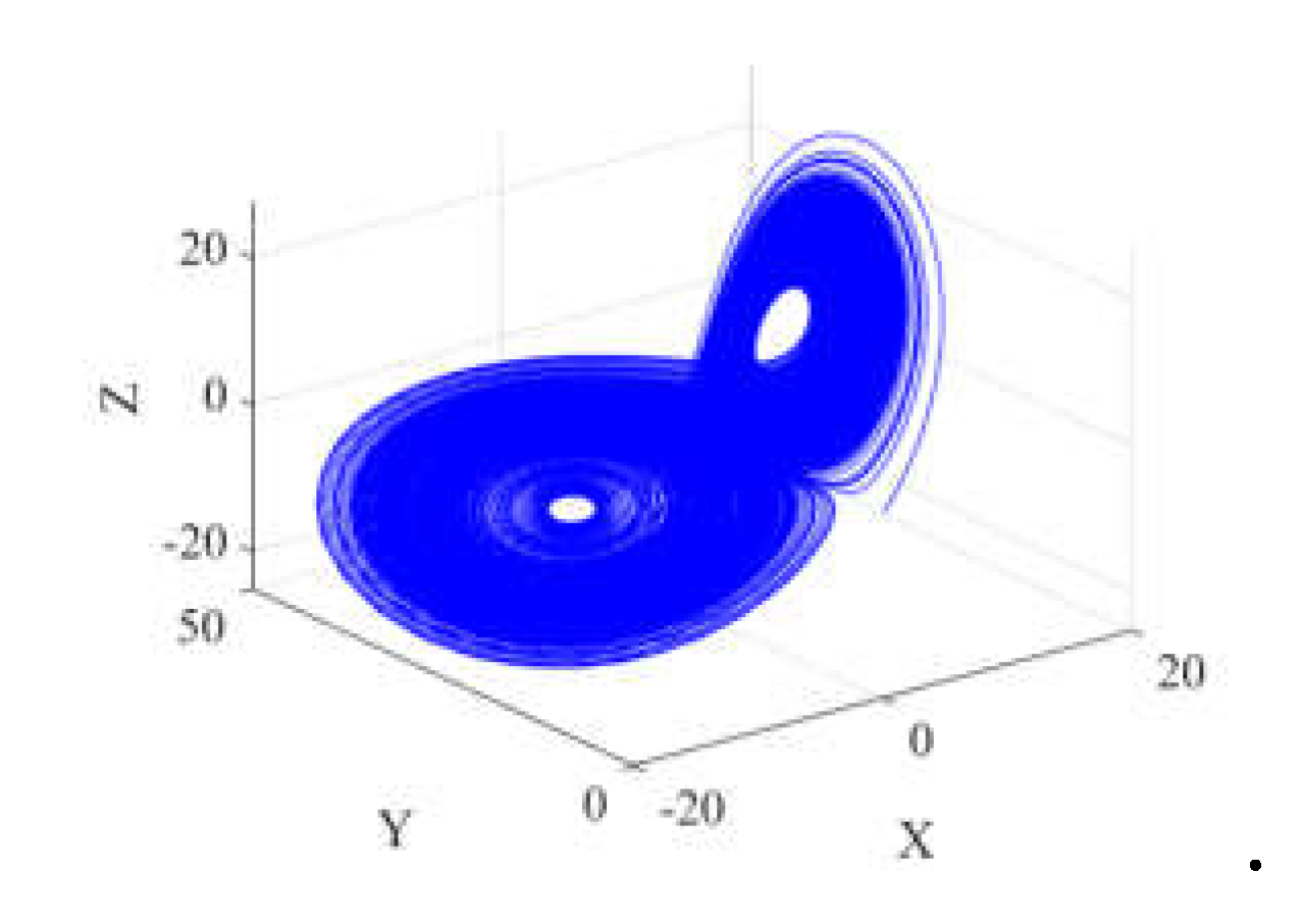
Figure 3.
Comparison between predicted and test set.
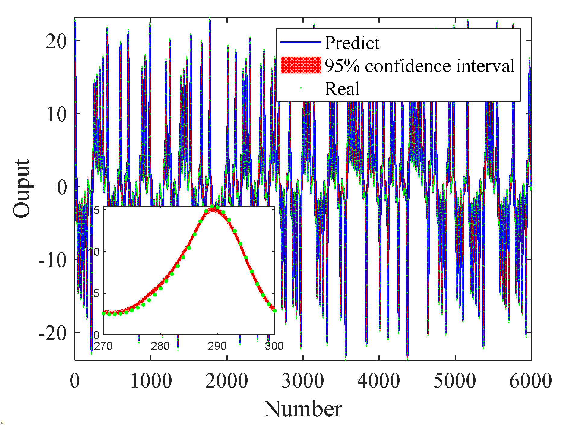
Figure 4.
Correlation between predicted and true value.
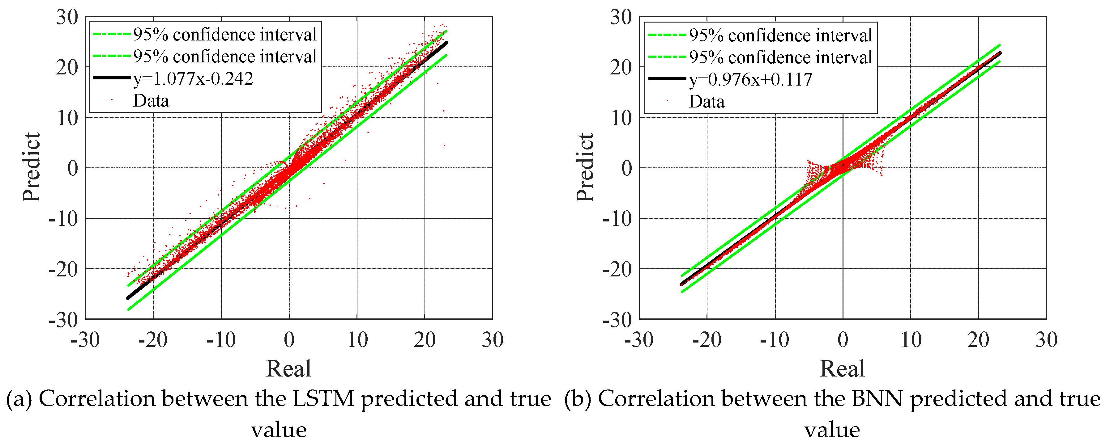
Figure 5.
Prototype monitoring system of the semi-submersible platform.
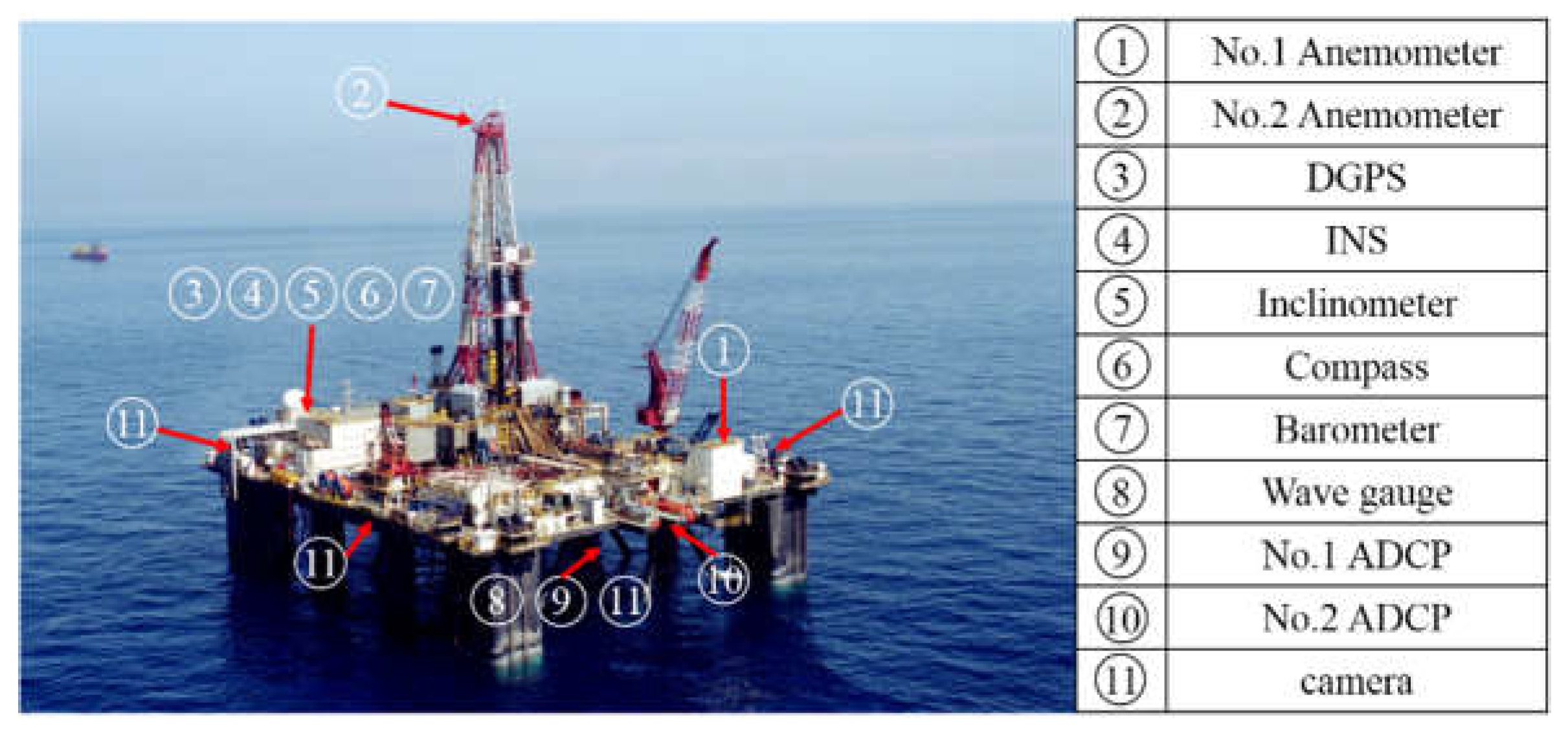
Figure 6.
Time history diagrams of 6 DOF motions of a semi-submersible platform.

Figure 7.
Time-frequency characteristics diagram of 6 DOF motions of a semi-submersible platform.
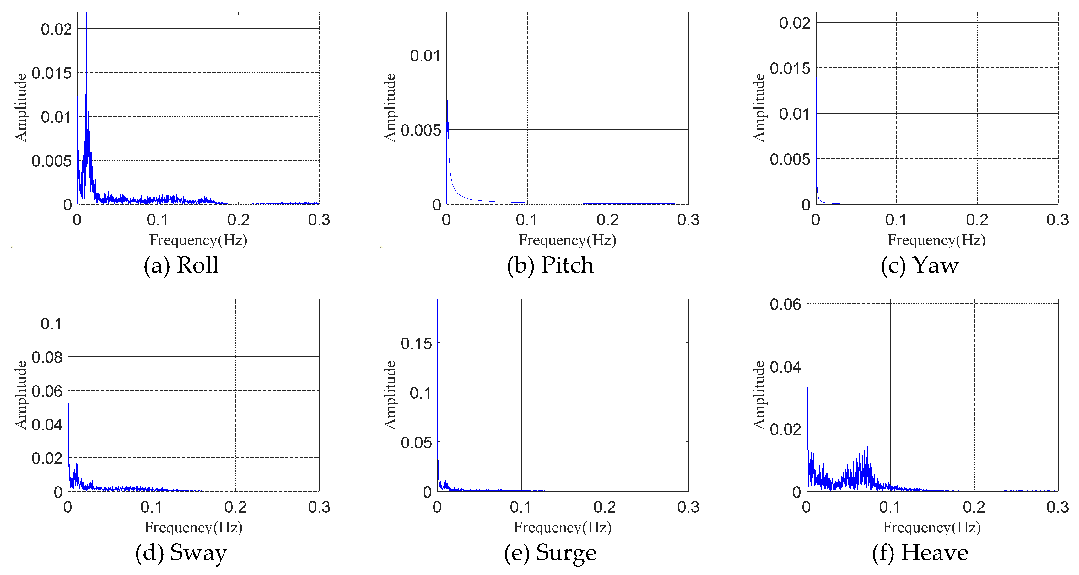
Figure 8.
Correlation coefficient of 6 DOF motions.
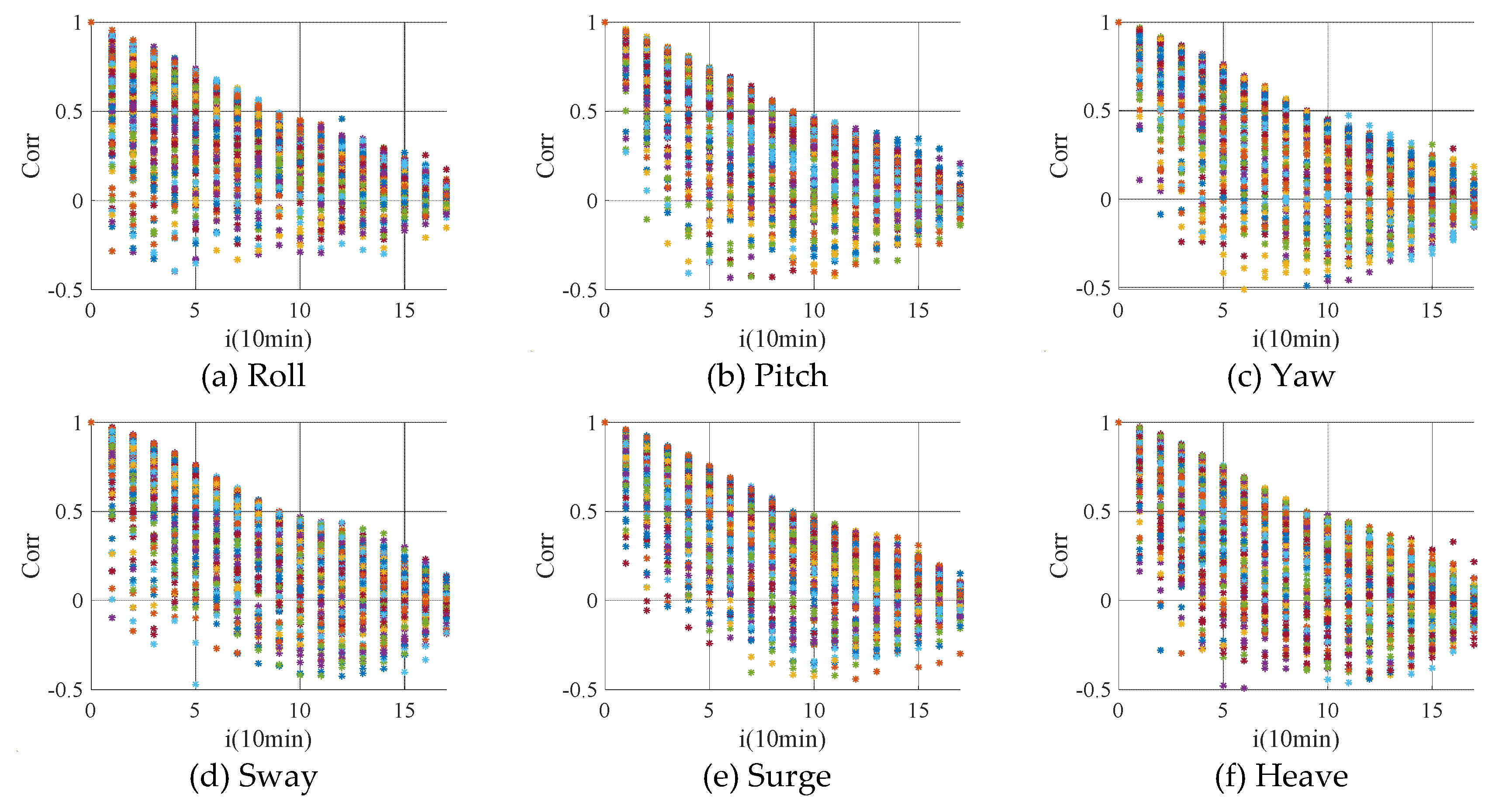
Figure 10.
Prediction process of the BNN.
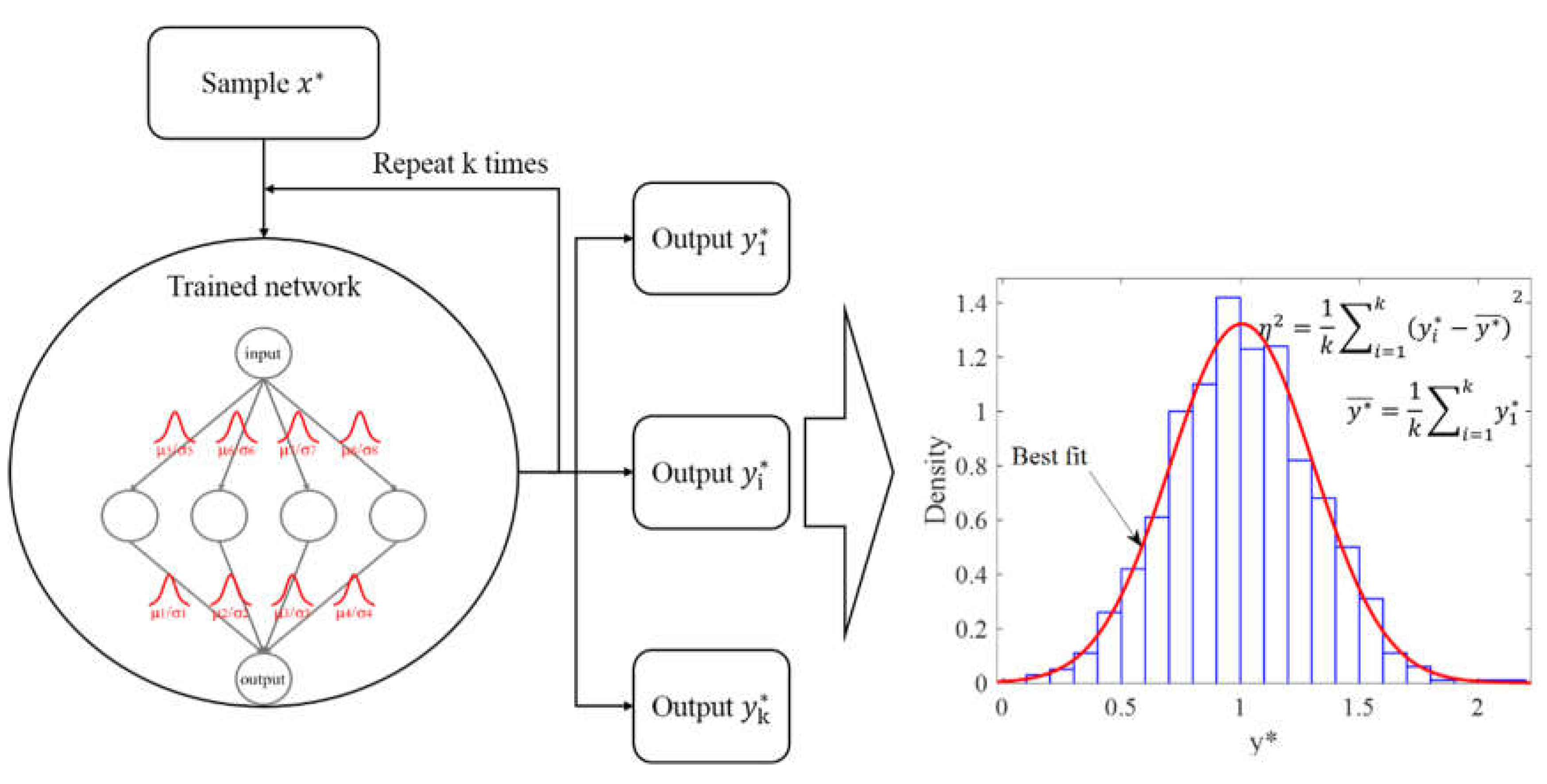
Figure 11.
The weight of the first five neurons in each layer of the network.
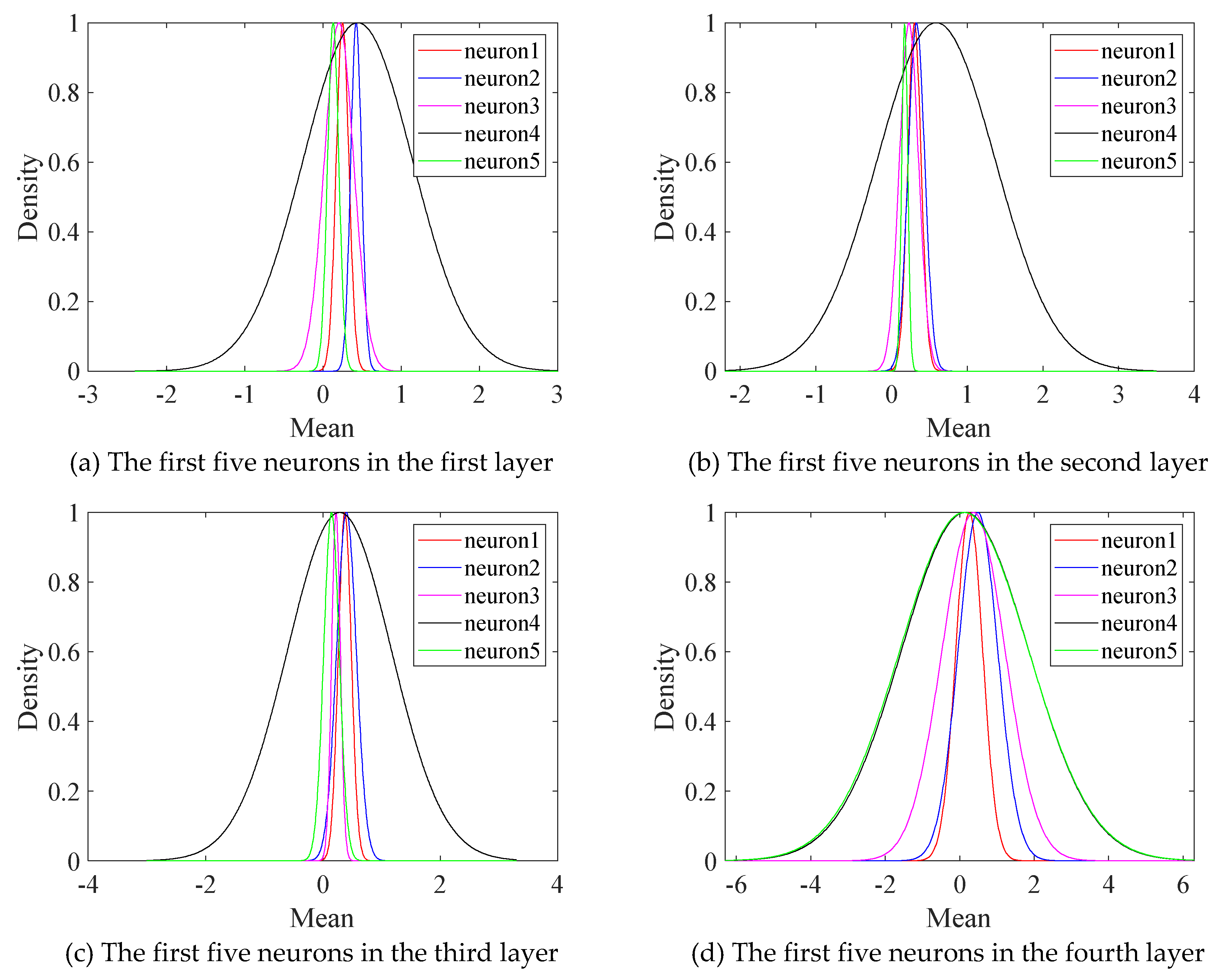
Figure 9.
Division of data sets.
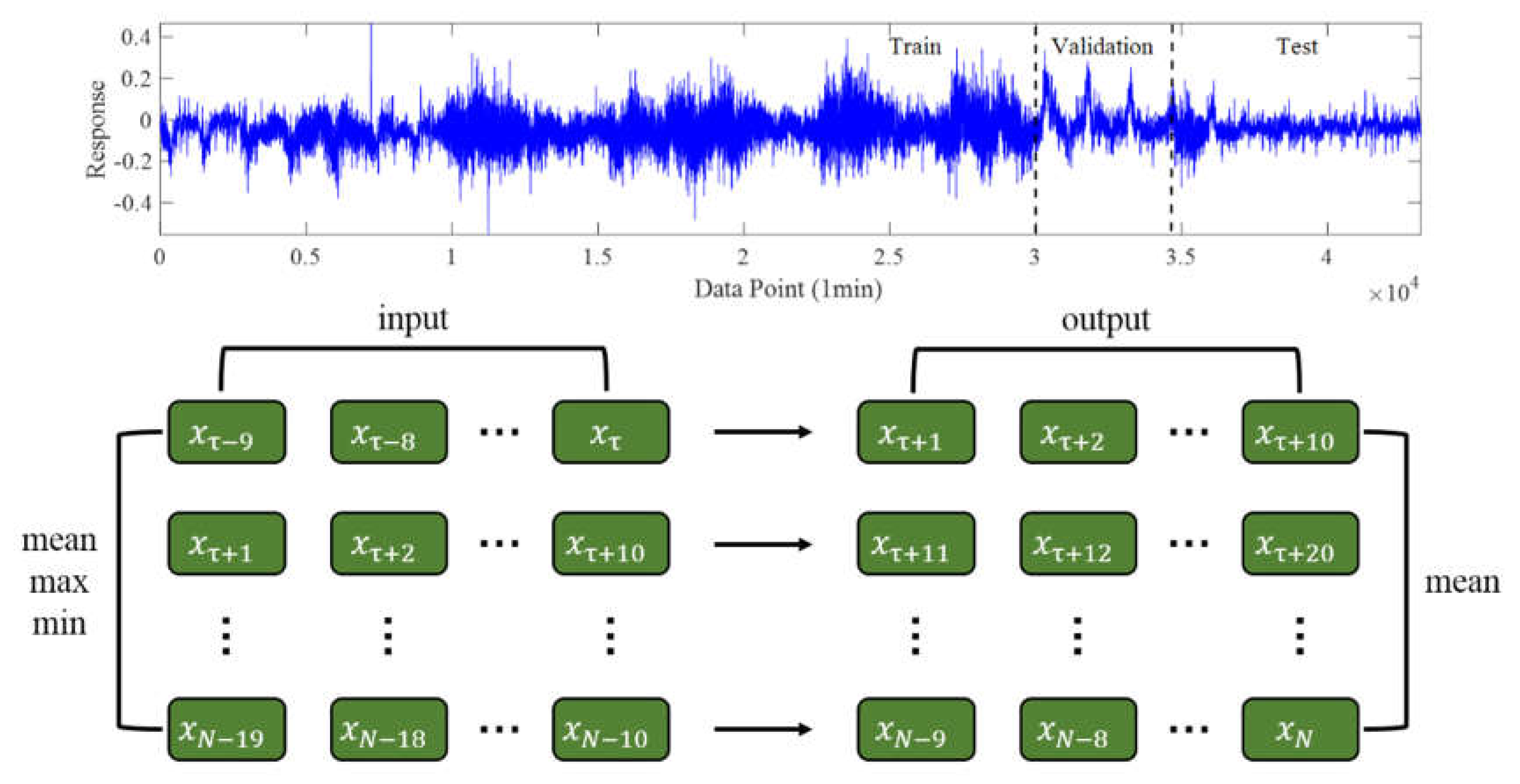
Figure 12.
Forecast results for the BNN.
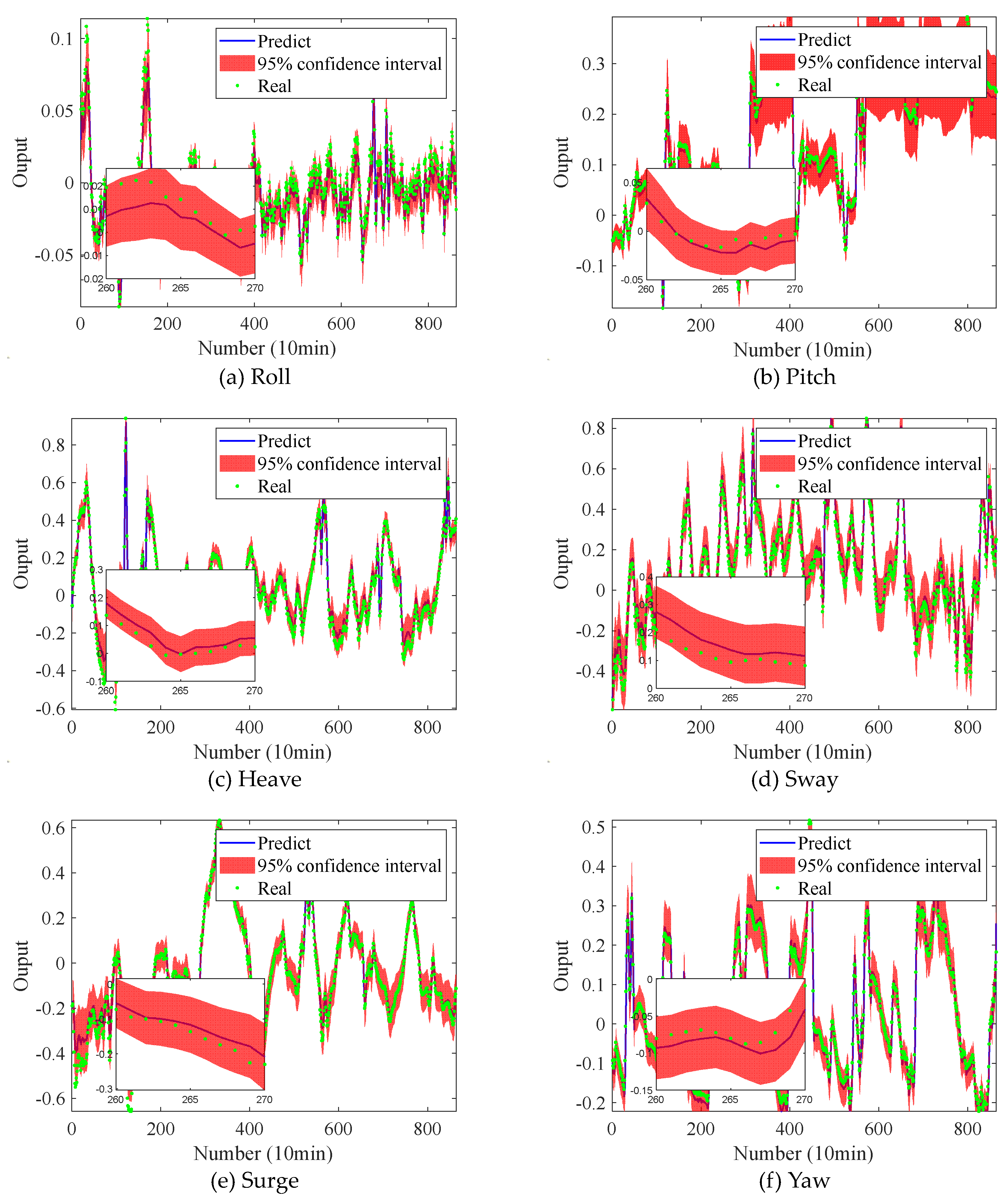
Figure 13.
Prediction error of the BNN and other models.
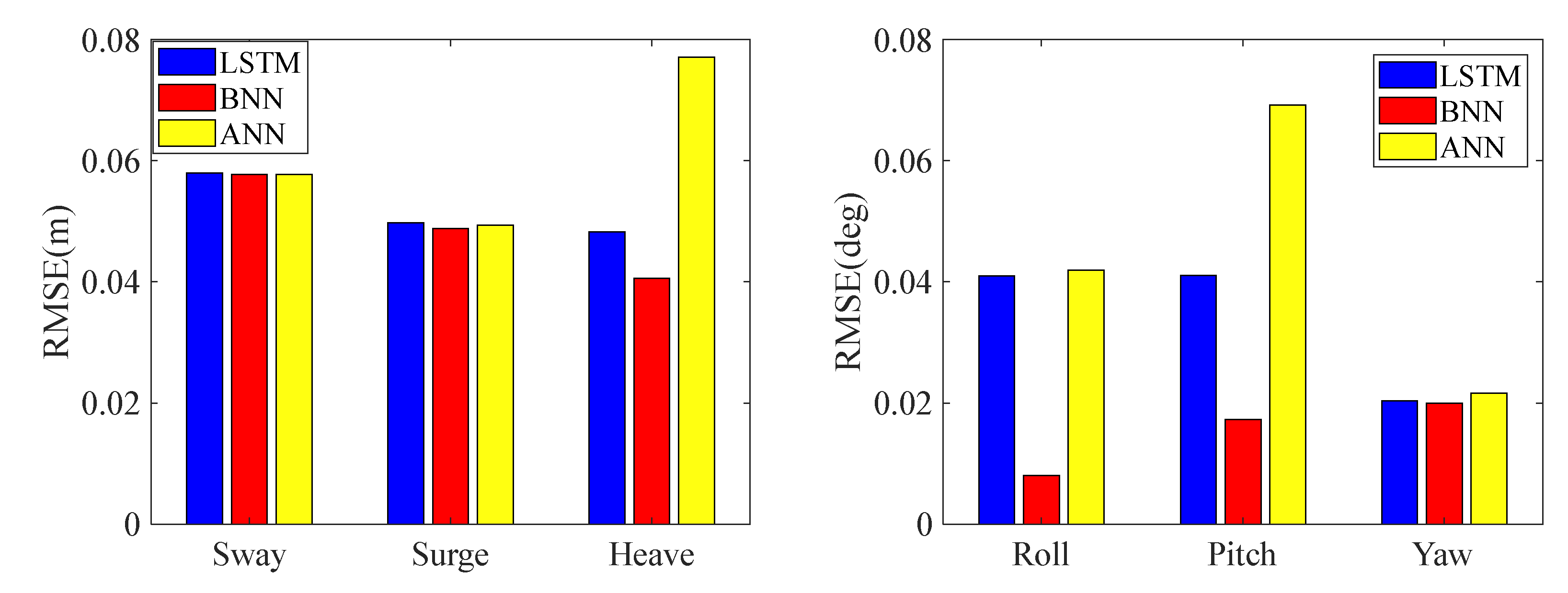
Figure 14.
Comparison between the predicted and the testing set data.
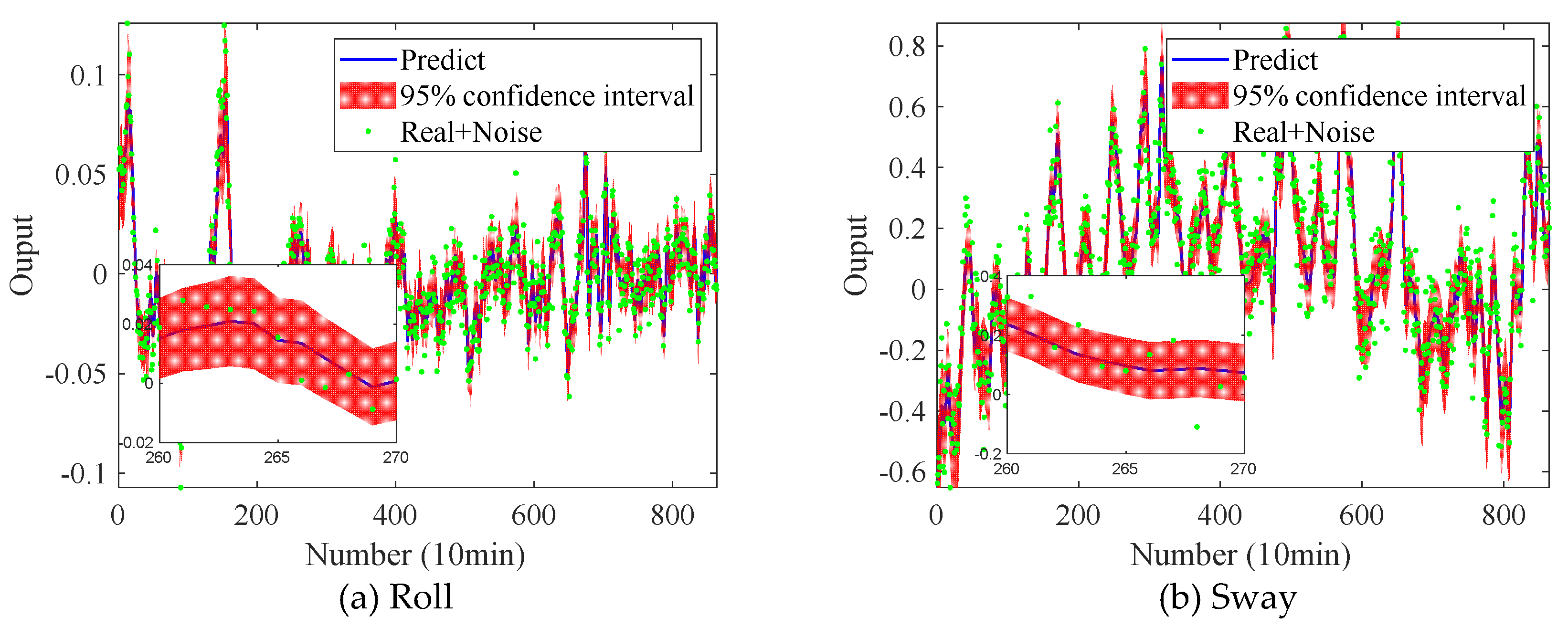
Figure 15.
Comparison between the predicted and the testing set data.
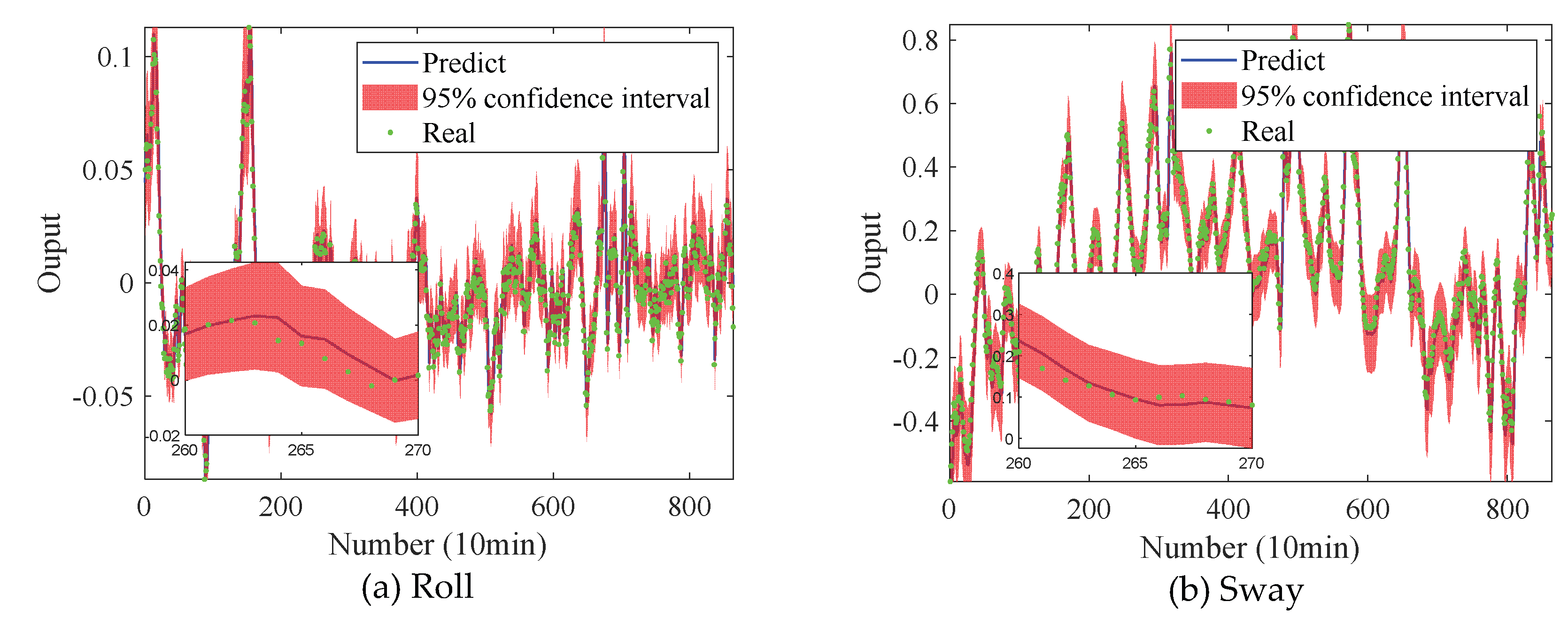

Table 1.
Precision comparison of different neural networks.
| Neural netwok | RMSE | R2 |
|---|---|---|
| LSTM | 1.412 | 0.974 |
| BNN | 0.855 | 0.990 |
Table 2.
Range and accuracy of monitoring information.
| Type | Sensor | Information | Range | Accuracy |
|---|---|---|---|---|
| Wind | Vane Anemometer | Wind speed, wind direction | 0-100 m/s, 0-360 deg |
0.1 m/s 0.2 deg |
| Wave | WaveGuide radar | Wave height, wave direction,Tp | 0-30 m, 0-360 deg | 0.01 m, 1 deg |
| Current | ADCP | Current velocity, current direction | ±10 m/s 0-360 deg |
0.1 m/s 1 deg |
| Linear motion | DGPS | Sway, surge | >0 m | 0.1 m |
| Heave | 0-3 m | 0.1 m | ||
| Angular motion | INS | Roll, pitch | ±30 deg | 0.01 deg |
| Yaw | 0-360 deg | 0.05 deg |
Table 3.
Hull parameters of a semi-submersible platform.
| Parameters | Value | Parameters | Value |
|---|---|---|---|
| Draft/m | 22.86 | Displacement/kg | 2.82×10⁷ |
| VCG from WL/m | -1.585 | Hull Weight/kg | 2.69×10⁷ |
| Roll Gyradius/m | 29.29 | Pitch Gyradius/m | 29.23 |
| Yaw Gyradius/m | 33.44 |
Table 4.
Mooring parameters of a semi-submersible platform.
| Line Segments | Grade | Length (m) | Wet Weight (kg/m) | Drag Coef. | Added Mass | Hydraulic diameter(mm) | Axial stiffness(KN) |
|---|---|---|---|---|---|---|---|
| Platform Chain | R4 | 221 | 276.80 | 2.4 | 1 | 120.65 | 1205408 |
| Riser Wire | SPIRAL STR. | 503 | 71.30 | 1.8 | 1 | 131.7625 | 1610149 |
| Ground Chain | R3 | 463-610 | 372.05 | 2.6 | 1 | 139.7 | 1583488 |
| Anchor Wire | SPIRAL STR. | 122 | 71.30 | 1.8 | 1 | 131.7625 | 1610149 |
Table 3.
Time scale with a correlation coefficient greater than 0.6.
| Motion | 80% Quantile | Corresponding Time Scale |
|---|---|---|
| Roll | 1, 0.602 | 0, 1 |
| Pitch | 1, 0.842, 0.675 | 0, 1, 2 |
| Yaw | 1, 0.843, 0.670 | 0, 1, 2 |
| Sway | 1, 0.794,0.667 | 0, 1, 2 |
| Surge | 1, 0.791,0.655 | 0, 1, 2 |
| Heave | 1, 0.777, 0.600 | 0, 1, 2 |
Table 4.
Network structure parameters of the BNN.
| Characteristic | Number of neurons | Layer of hiding | Epoch | Learning rate | Variance of prior | Activation function |
|---|---|---|---|---|---|---|
| Number | 64 | 2 | 2000 | 0.1 | 1 | sigmoid |
Table 5.
RMSE of validation set and testing set.
| Roll (deg) | Pitch (deg) | Yaw (deg) | Sway (m) | Surge (m) | Heave (m) | |
|---|---|---|---|---|---|---|
| Validation set | 0.0218 | 0.0233 | 0.0543 | 0.0540 | 0.0545 | 0.0858 |
| Testing set | 0.0080 | 0.0173 | 0.0200 | 0.0577 | 0.0488 | 0.0405 |
Table 6.
True value included in 95% confidence interval and R2.
| Motion | Percent (100%) | R2 |
|---|---|---|
| Roll | 92.1 | 0.915 |
| Pitch | 96.2 | 0.987 |
| Yaw | 97.0 | 0.984 |
| Sway | 95.0 | 0.957 |
| Surge | 96.4 | 0.963 |
| Heave | 96.6 | 0.968 |
Table 7.
Precision of the LSTM and the BNN.
| Roll (deg) | Pitch (deg) | Yaw (deg) | Sway (m) | Surge (m) | Heave (m) | |
|---|---|---|---|---|---|---|
| LSTM | 0.0409 | 0.0410 | 0.0204 | 0.0579 | 0.0497 | 0.0482 |
| ANN | 0.0419 | 0.0692 | 0.0216 | 0.0577 | 0.0493 | 0.0771 |
| BNN | 0.0080 | 0.0173 | 0.0200 | 0.0577 | 0.0488 | 0.0405 |
Table 8.
True value included in 95% confidence interval R2 and RMSE.
| Roll | Percent (100%) | R2 | RMSE | |
|---|---|---|---|---|
| Roll | Native | 92.1 | 0.915 | 0.008 deg |
| Native + noise | 69.9 | 0.815 | 0.013 deg | |
| Sway | Native | 95.0 | 0.957 | 0.058 m |
| Native+noise | 66.0 | 0.849 | 0.114 m |
Table 9.
True value included in 95% confidence interval R2 and RMSE.
| Roll | Percent (100%) | R2 | RMSE | |
|---|---|---|---|---|
| Roll | Native train | 92.1 | 0.915 | 0.008 deg |
| Native + noise train | 93.6 | 0.915 | 0.008 deg | |
| Sway | Native | 95.0 | 0.957 | 0.058 m |
| Native+noise train | 95.37 | 0.960 | 0.056 m |
Disclaimer/Publisher’s Note: The statements, opinions and data contained in all publications are solely those of the individual author(s) and contributor(s) and not of MDPI and/or the editor(s). MDPI and/or the editor(s) disclaim responsibility for any injury to people or property resulting from any ideas, methods, instructions or products referred to in the content. |
© 2026 by the authors. Licensee MDPI, Basel, Switzerland. This article is an open access article distributed under the terms and conditions of the Creative Commons Attribution (CC BY) license.
Copyright: This open access article is published under a Creative Commons CC BY 4.0 license, which permit the free download, distribution, and reuse, provided that the author and preprint are cited in any reuse.


