
Submitted:
06 June 2025
Posted:
09 June 2025
You are already at the latest version
Abstract
Accurate short-term wave forecasting is critical to floating marine structures' efficient and safe operations as well as their active control using models (e.g., digital twins) that rely on real-time, phase-resolved ocean wave loading. For moored, i.e., quasi-stationary systems informed by environmental sensors (e.g., waverider buoys, wave-sensing LIDAR), challenges arise when upstream sensor data is missing, sparse, or phase-shifted due to drift. This study investigates the resilience and performance of machine learning models—specifically TiDE and LSTM—for forecasting phase-resolved ocean surface elevations under various scenarios of data loss and uncertainty. We introduce $\tau$-trimmed models, which dynamically adapt the prediction horizon based on uncertainty thresholds derived from historical forecasts. Numerical wave tank (NWT) and wave basin experiments are used to benchmark model performance under short- and long-term data masking, spatially coarse sensor grids, and upstream phase shifts. Results show that $\tau$-trimmed models consistently reduce forecast errors and uncertainty, particularly under degraded conditions. While LSTM models achieve lower average errors, TiDE models—especially the conservative variant—exhibit greater robustness and efficiency. Phase shifts in upstream data are shown to be more detrimental than masking alone. These findings inform the design of resilient, uncertainty-aware wave forecasting systems suited for realistic offshore sensing environments.
Keywords:
machine learning
; uncertainty quantification
; dynamic prediction horizon
; data masking
; phase shift
; TiDE model
; LSTM
; floating sensors
; offshore monitoring
; digital twin
1. Introduction
Ocean waves can cause large forces on offshore marine structures, and hence large motion of floating structures, that affect both their efficient operations and fatigue life. Predicting wave propagation in space and time has been the focus of many studies, using a variety of both physics-based and, more recently, data-driven models. Away from shore, irregular ocean waves have typically been represented by linear superposition, leading to a spectral representation in the frequency domain, with related spectral and statistical parameters (e.g., significant wave height, peak spectral period, etc...). This approach has help determining, or forecasting, extreme sea-state parameters for various analyses and design purposes. However, a spectral representation lacks phase, i.e., individual wave information, which becomes extremely important for many applications such as optimizing motion control strategies of a floating structure. For example, Li et al. [1] concluded that wave energy converters have increased efficiency when their control mechanism assimilates phase-resolved wave predictions; the latter also must be used for active control strategies of floating wind turbine systems [2,3]. Seaborne additive manufacturing (SAM) and underwater 3D printing are other examples where the short-term phase-resolved predictions are crucial to ensure accurate operations at sea [4,5].
Physics-based predictions of ocean wave fields require using a physically relevant model and “inverting” it to fit it to observations (i.e., by minimizing the mean square error of simulated to measured) (e.g., [3,6,7]). This is called the nowcast, and once a nowcast of the ocean surface is obtained on the basis of some measurements, the fitted model can then be used to perform a forecast of the wave surface elevation expected at the location and future time of interest[8,9]. For models based on linear wave theory (LWT), the predictable space-time zone can be determined based on the wave group velocities of the fastest and slowest components of the reconstructed wave field [7,10,11].
For severe sea-states, more advanced wave models have been developed that account for wave nonlinearity (to some order), which affects both wave shape and phase speed (e.g., [7,12,13,14]) For instance, Grilli et al. [6] and Nouguier et al. [13] developed nonlinear free surface reconstruction algorithms, using an efficient Lagrangian-based Choppy model [12,14], and validated them for 1D and 2D irregular surface waves, using simulated LIDAR data to create relevant data sets. This approach was further developed by Desmars et al. [7], who conducted an experimental and numerical assessment to evaluate ocean wave prediction algorithms tested on non-uniformly distributed 1D data similar to data sampled from a LIDAR camera. They confirmed that the prediction accuracy converged as the amount of input data involved during the inversion process increases; similar experiments and Choppy-based wave forecasting were performed by Albertson et al. [3], for actively controlling the motions of a floating marine structure. More recently, Kim et al. [15] performed experiments and applied and validated these models for 2D data, reaching the same conclusions.
While physics-based models can achieve near real-time reconstruction and predictions as long as nonlinear effects are weak or negligible [3,15,16,17], the reconstruction problem (i.e., determining the state of the wave field, wave components, nonlinear couplings, etc.) and the time it takes to invert, integrate equations, and generate predictions are major challenges to the practicality of using such models in severe sea-states [18], unless powerful computational hardware is embarked onto the marine structure. As an alternate approach, advanced machine learning tools, when properly trained on relevant data, have been shown to accelerate these processes and even enhance the accuracy of the predictions [19,20]. For example, Jörges et al. [21] used a Long-Short-Term-Memory (LSTM), a recursive neural network (RNN) type, to predict nearshore significant wave heights. Other researchers have focused on utilizing ML-models to forecast phase-resolved wave time series [18,22,23]. Kagemoto [24] developed a LSTM model to predict experimental and numerical irregular wave trains and extrapolated their model to forecast the motion response of a floating body. They concluded that the model is capable of producing reasonably accurate predictions in spite of nonlinear effects present in the data. Duan et al. [23] constructed a neural network-based wave prediction model (ANN-WP) where they utilized experimental data to train, validate, and conduct comparison studies with linear wave prediction (LWP) algorithms and proved that ANN-WP is superior in performance to LWP.
In other work, some studies have demonstrated that uncertainty quantification (UQ) can be used in conjunction with phase-resolved real-time wave prediction to: 1) expand the predictable zone, which is otherwise quite conservative when using LWT-based models, 2) inform the control algorithm of the level of confidence to perform a control action based on an uncertainty score for a given predicted value [20]. Silva and Maki [25] have used similar uncertainty quantification using the Monte Carlo dropout approach proposed by Gal and Ghahramani [26] to perform system identification for 6-DOF ship motions in waves under various upstream wave probe setup. Law et al. [27] used a higher-order spectral-numerical wave tank (HOS-NWT) method developed by Bonnefoy et al. [28], Ducrozet et al. [29] to generate datasets to train their artificial neural network for two wave steepness values, a limiting and a mean steepness values. Harris [30] developed a data-driven model that is faster than real-time. Their choice of machine learning approach was the Time-Series Dense Encoder (TiDE) as it has shown good balance between model complexity, stability, and computational time.
Even though prior research has demonstrated the capability of machine learning (ML)-models to generate accurate and rapid forecasts of phase-resolved ocean wave fields, either through numerical simulations or experimental campaigns, little attention has been given to their robustness and generalizability across diverse ocean conditions and varying upstream data availability. In most existing studies, the number and placement of upstream wave probes are fixed and highly controlled. In contrast, real-world deployments—particularly in deep water—often involve dynamic or uncertain probe locations due to drifting buoys. This variability can significantly alter the spatial distribution of available data used for wave reconstruction. The issue is further exacerbated when optical sensors such as LIDARs are employed. Data loss may also occur due to equipment malfunction, shadowing effects, or the inability to detect the free surface location reliably. Despite these challenges being common in practical applications, sensitivity analyses of ML-model performance under such conditions remain largely unexplored. This work aims to address this gap by evaluating the resilience of ML-based wave field reconstruction methods under realistic, variable data acquisition scenarios.
2. Methodology
This paper presents results and sensitivity analysis conducted on both experimentally and numerically generated data. We design the problem by building appropriate ML-models and test them under different scenarios simulating various conditions after fitting them.
2.1. Experimental and Numerical Setup
The experimental campaign took place at the Harold Alfond wind-wave (W2) basin at the Advanced Structures and Composites Center located at the University of Maine. The wave basin layout and the various probes used for various analysis in this paper are presented in Figure 1. In experiments, a 1:70 Froude scale was assumed.
The wave basin was numerically replicated using the Higher-Order Spectral Numerical Wave Tank (HOS-NWT) model developed by Bonnefoy et al. [28], Ducrozet et al. [29], hereafter referred to as NWT. The simulated tank dimensions are 30 m in length, 10 m in width, and 5 m in depth. A wave absorbing beach is positioned at 85% of the tank length and configured with an absorption strength of 90%. In the experimental setup, five wave probes were deployed—two closely spaced upstream, two downstream, and one located furthest downstream. To enhance spatial resolution in the numerical model, additional virtual wave probes were incorporated, resulting in a total of 25 probes distributed primarily at 0.5 m intervals.
2.2. Wave Forecasting Model Development
Two machine learning-based models were investigated in this study. These models were trained using available data from either physical experiments (EXP) or the Numerical Wave Tank (NWT) simulations. During testing, past data from all sensors were provided as input. The internal mapping learned during training is designed to correlate free surface elevations recorded by upstream probes with their subsequent propagation toward downstream locations. As a result, the models can forecast future wave elevations downstream based on historical probe measurements.
The first model is a recurrent neural network (RNN) of the multivariate Long Short-Term Memory (LSTM) type. LSTMs are well-regarded for their ability to retain both short- and long-term temporal dependencies with a forget gate to regulate the flow of past information, making them effective for time series forecasting [32]. The second model is Time-series Dense Encoder (TiDE), a state-of-the-art deep learning architecture proposed by Das et al. [33] designed to be more efficient and to potentially outperform more complex models. For time series manipulation and model implementation, we used the open-source Python library Darts, developed by Unit8 SA [34].
Both models were trained using consistent hyperparameter settings: 1,000 epochs, a batch size of 32, a hidden layer size of 100, a dropout rate of 0.1, and an optimizer learning rate of 0.001. A probabilistic forecasting framework was adopted through the use of the Laplace likelihood, which enables the models to produce a distribution of likely outcome to generate uncertainty bounds for each prediction. Performing uncertainty quantification (UQ) is crucial in the context of phase-resolved, ocean wave forecasting, as it allows the systematic evaluation of confidence levels associated with each prediction. This is particularly useful when control systems are influenced by phase-resolved predictive models to reduce risks and high fatigue on these systems.
In both models, the same input-output structure was employed: a historical sequence of length, m is used to forecast a future horizon of n steps. A ratio of is utilized. This implies, for a prediction horizon of , the model observes two seconds of past data to predict one second ahead. The value of n was initially set to 120. With a temporal resolution of , this corresponds to a forecasting horizon of . This selection was informed by the range of group velocities, associated with the sea-state under consideration, given all numerical probes are active. We use group velocity since the energy content of the wave field propagates downstream with the group velocity, given in LWT by:
where and k denote the angular wave frequency and wavenumber, respectively, and h is the water depth. In sufficiently deep water conditions (i.e., ), the group velocity asymptotically approaches half the wave phase velocity, .
Since the multivariate forecasting problem is complex to define, we present here a uni-variate counterpart for simplicity. We create a forecast of the surface elevation target, y, given a known dynamic history of itself and other covariates, x, which can be written as:
In the TiDE model, the upstream probes were considered as covariates (meant to help build the prediction but their signal is not included in the forecast). However, the LSTM used all probes as variables. Due to causality, this would generate wrong forecasts at the most upstream probes and the propagation of that error downstream is possible.
To quantify the error between the predicted variable, y, and the observed signal, , we calculated the Mean Absolute Error (MAE) metric as:
Two sea-states were being investigated in this research, a moderate one (SS1) and a severe one (SS2), both described by a JONSWAP spectrum using three parameters: the significant wave height, , peak wave period, , and the peak enhancement factor, . These parameters are detailed in Table 1.
2.3. Data Masking
We simulates two scenarios concerning the input data fed into the models. The first involves a temporal Monte Carlo dropout (or masking) of input signals from upstream buoys, representing either short- or long-term data loss. Short-term masking affects multiple sensors and occurs frequently in both space and time, but only for short durations, . This setup evaluates challenges such as intermittent signal acquisition—caused, for example, by low-visibility conditions affecting LIDAR—or shadowing effects. In contrast, long-term masking of a limited number of sensors tests the model’s robustness in maintaining predictive accuracy under conditions of sensor malfunction, power loss, or prolonged shadowing effects.
This methodology addresses a key challenge in data-driven modeling: handling highly irregular spatiotemporal input, such as LIDAR data, and converting it into a structured format suitable for models requiring uniform input. To simulate data loss, time series signals were first divided into windows. Each window was assigned a random number between 0 and 1. If this number exceeds a given probability threshold, , masking was applied. Higher values of increase the likelihood of masking across more windows. Figure 2 illustrates the adopted masking strategy.
The second scenario introduces a temporal phase shift to signals from upstream buoys. This simulates real-time data collection from floating wave sensors, which may drift and change position due to ocean currents and wave forces, resulting in positive or negative phase shifts in the recorded signals. Figure 3 shows an example of this effect. We assess model resilience to such phase discrepancies and quantify the corresponding degradation in predictive performance.
2.4. τ-Trimmed Models
Zhang et al. [20] used uncertainty-based parameterization to define a predictable zone for wave forecasting. In this study, we extended this approach to multivariate signal processing, incorporating uncertainty levels derived from historical forecasts.
First, we computed the uncertainty level for each target signal, as follows:
where and represent the 97.5th and 2.5th percentiles of the predicted distribution for . We then defined a minimum uncertainty threshold,
below which the forecast was considered reliable, i.e., when ; where M is the number of output signals, and and are the minimum and maximum observed uncertainties for each signal j.
Models that adapt their prediction horizon based on this threshold were referred to as -trimmed models, for which , the horizon, was computed as the time during which the uncertainty stays below . For each historical forecast, this time horizon was computed by:
- smoothing the uncertainty signal using a 1D convolution with a Gaussian kernel,
- finding the total time during which,, and
- summing the number of valid time steps and multiplying by the time resolution to obtain .
Two types of -trimmed models were defined:
- Moderate-type: for which was selected based on the peak of the distribution of valid horizons (or the average of all peaks in case of multivariate).
- Conservative-type: which used the smallest that occurred in the distribution, beyond which the uncertainty threshold can be violated.
Figure 4(a) shows the resulting distribution (via violin plots) for the TiDE model applied to numerical wave tank data, focusing on the most downstream probes. Figure 4(b) illustrates a single forecast stride contributing to this distribution, highlighting how increases downstream as the model benefits from accumulating upstream information. This trend is also reflected in the violin plots.
3. Results
In the following, we present results of applying the machine learning models developed in this study to numerical and experimental wave data, and evaluate their performance and resilience under various input masking (i.e., data decimation) scenarios.
3.1. Numerical Wave Tank Investigation
Results of the HOS-NWT model provide highly resolved data at sensor (probe) locations, resulting in rich datasets that improve the predictive model learning and prediction accuracy. Only the SS1 sea-state was considered in this section (Table 1). The following tasks were conducted:
- Benchmarking the baseline model performance against uncertainty-based -trimmed models;
- Evaluating the effects of short- and long-term input data masking on prediction accuracy;
- Comparing a covariate-based model (TiDE) with a non-covariate-based model (LSTM).
To conduct a comprehensive sensitivity analysis, we defined four levels of masking probability thresholds, . When , no masking is applied—this represents the ideal case where all probes function correctly and no randomness is introduced. In contrast, higher values increase the likelihood of masking across time windows. Short- and long-term masking durations are defined by the window length , as illustrated in Figure 2. Specifically, for SS1-related data, short-term masking used s, while long-term masking uses s.
Figure 5 and Figure 6 show the performance of the TiDE and LSTM models, respectively, based on NWT data. Each figure presents the MAE metric (Eq. 3) between observed and predicted values for the most downstream sensors. The top row of subplots corresponds to short-term data masking, while the bottom row corresponds to long-term masking. Within each row, the left subplot shows results for the baseline model, and the right subplot shows results for the corresponding -trimmed model.
3.1.1. Baseline and -Trimmed Models Comparison
A general trend can be observed when comparing the left and right subplots in Figure 5 and Figure 6: the -trimmed models consistently yielded lower MAE values compared to the baseline models. However, both model types converged to similarly low error levels as waves propagate downstream, suggesting a reduced benefit of applying -trimming models to later spatial positions.
Table 2 and Table 3 provide MAE values for probes p19 and p24 under short-term masking scenarios, for the TiDE and LSTM models, respectively. In both tables, the last column reports the relative difference in MAE values between the baseline and -trimmed models. Negative values indicate that the -trimmed model outperforms the baseline model for the same wave data and masking scenario. The largest observed improvement occurred at probe p19 for , where the -trimmed LSTM model achieved a 56% reduction in error. As increased—meaning more masking is applied to probes—this performance gap narrowed. This is expected, as both models are increasingly challenged by the loss of input data.
3.1.2. Impact of Short-Term vs. Long-Term Data Masking on Model Accuracy
Figure 5 and Figure 6 show the mean and 95% confidence intervals based on 10 repeated trials (a preliminary sensitivity analysis—not shown here—indicated that 10 repetitions were sufficient to produce representative results). The confidence intervals, visualized as transparent bands around the mean, were consistently wider for long-term masking scenarios compared to short-term ones, regardless of the model used. This indicates that extended data loss has a more detrimental and variable impact on forecasting accuracy than intermittent, shorter-term masking.
3.1.3. Comparison of the TiDE and LSTM Model Results
Both the TiDE and LSTM models performed well under the tested masking conditions. However, notable differences emerged in error variation spatially. Specifically, TiDE model results exhibited a more pronounced error in upstream targets (e.g., p19), as seen in Figure 5(a) and (c). In contrast, LSTM model results showed relatively uniform error levels from upstream to downstream targets, as shown in Figure 6.
According to Table 2, TiDE model results had an error difference exceeding 50% between p19 and p24 when , which decreased to 35% when . LSTM model results, on the other hand, yielded a smaller difference of 34% for , which narrowed substantially to only 3% for (Table 3). This suggests that LSTM is more consistent across locations, while TiDE may be more sensitive to input data availability, especially for upstream targets.
3.2. Experimental Investigation
In the following, we present results of applying the machine learning models to experimental data acquired in the University of Maine basin. While the numerical investigation demonstrated the models’ ability to forecast downstream free surface elevations with high spatial resolution, it is equally important to assess model performance under more constrained conditions—specifically, when data is only available on a coarser spatial grid of sensors/probes and additional input masking is applied.
Data acquired from experiments run for both sea-states SS1 and SS2 described in Table 1 were considered in this analysis. Two variants of the TiDE model were developed to explore differences in the predictable zone. The first follows the moderate-type strategy used in the numerical study, while the second adopted a more conservative approach, deemed necessary due to the reduced number of upstream probes. These two variants are illustrated schematically in Figure 7.
For the moderate-type model, the dynamic prediction horizons were computed as s for SS1 and 34 s for SS2. The conservative-type model used shorter horizons of s and 20 s, respectively. When overlaid as horizontal dashed lines on the space–time (upper) plots of Figure 7, these values aligned well with the predictable zone shadows inferred from the upstream probes (using LWT group velocities). Specifically, the moderate horizon coincided with the predictable zones generated by the first and second probes, while the conservative horizon aligned with zones generated by the third and fourth probes—those closest to the target location. This alignment suggests that relying on more distant upstream data may introduce higher uncertainty due to wave dispersion effects, as waves travel downstream.
The group-velocity-based predictable zone shadows shown in Figure 7 (upper space-time plots) were computed using the minimum and maximum group velocities with Eq. 1, applied over a 50-second moving window. It is also worth noting that waves in SS2 propagate faster (as they are longer-period), which naturally results in shorter prediction horizons for both model types.
3.2.1. Sensitivity to Data Availability Under Spatially Coarse Grid Constraint
As in the previous section, we assessed the models’ performance under both short- and long-term data masking scenarios. Here, we set the masking probability threshold to and varied only the masking duration. Figure 8 presents the resulting error levels for both the moderate- and conservative-type prediction horizons. The error bars represent the 95% confidence intervals.
Figure 8(a) shows that the overall MAE levels remain relatively high, yet comparable to those from the NWT-based analysis. This indicates that the models were still capable of delivering phase-resolved wave forecasts even when operating under coarser spatial resolution—i.e., with fewer upstream probes.
To further illustrate the effect of long-term data loss on wave forecast accuracy, Figure 9 shows the instantaneous MAE between the original signal and the model’s historical forecast, along with a smoothed MAE error curve, using a Gaussian filter. Two scenarios are presented: (1) under healthy operating conditions where all covariates were active, and (2) when a single covariate (the third upstream probe) went offline. The results clearly show increased error spikes and a higher smoothed error level when the covariate was unavailable, highlighting the importance of upstream sensor reliability.
3.3. Phase Shift Effects of Upstream Data
To simulate the effects of drifting ocean sensors, a phase shift mask was applied to the signals from the first and second experimental wave probes (out of five). A sensitivity analysis was then performed by varying the introduced phase shift, , to evaluate its impact on wave forecast accuracy for both the moderate- and conservative-type models.
Note that the magnitude of the phase shift corresponds to the physical displacement of the buoy within its watch circle governed by the sea-state. For example, the wave celerity (i.e., phase velocity) of SS1 is approximately 14 m/s at the peak period. Thus, a 1-second phase shift implies a horizontal displacement of about 14 m, assuming frozen-phase wave propagation. Given realistic mooring constraints, high phase shifts are unlikely for properly moored buoys. Nevertheless, to evaluate model robustness, we swept values across a broad range, from to seconds.
Thus, Figure 10 shows how the MAE varies as a function of phase shift, , applied to the first two upstream probes. The results indicated a substantial sensitivity of the MAE to phase perturbations, especially for the moderate-type model. The conservative model maintained lower error levels overall.
4. Discussion
The numerical investigation of wave forecasting errors using the various models demonstrated that when sufficient upstream data is available, the machine learning models are capable of accurately forecasting phase-resolved ocean waves, even in the presence of data loss. However, the role of uncertainty quantification is critical: without constraining prediction uncertainty, errors can exceed acceptable thresholds, potentially jeopardizing the reliability of downstream applications, such as wave-aware control systems.
Results showed that long-term data masking leads to significantly wider uncertainty bounds compared to short-term masking. This indicates that prolonged data loss introduces higher variability in model outputs. The use of -trimmed models effectively mitigates this effect, maintaining lower error levels by dynamically adjusting the prediction horizon based on previous forecast uncertainty levels.
Although the LSTM model exhibited lower average error values (Figure 6), it also suffered from causality-related issues. Specifically, erroneous predictions at the most upstream probes can propagate downstream if intermediate probes do not provide sufficient supplementary information. Moreover, LSTM models require longer training times due to the need to forecast multiple targets simultaneously. TiDE models, in contrast, provide a good balance between accuracy and computational cost, as was also pointed out by Harris [30].
TiDE models showed strong performance under densely spaced upstream probes. However, under experimental conditions with coarser spatial probe resolution and more energetic sea-states, the moderate-type model exhibited a degraded accuracy. To address this, we introduced a conservative-type -trimmed model with shorter prediction horizons, derived from uncertainty thresholds. This version demonstrated greater resilience to both data loss and phase shifts.
The phase shift analysis reveals that drifting upstream probes—which alter the temporal alignment of input signals—can degrade the wave forecast accuracy downstream, more severely than complete data masking. This insight suggests the potential value of dynamically deactivating unreliable sensors in real time, rather than feeding uncertain signals into the models. Moreover, for data acquisition systems with irregular spatial or temporal coverage—such as LIDAR—the model should be trained assuming a maximum upstream sensor grid. Irregularities can then be handled via dynamic masking to reflect real-time sensor availability based on acquired data locations.
Overall, these results support the development of flexible, uncertainty-aware forecasting models that are robust to realistic operational challenges such as missing data, probe drift, and coarse spatial resolution in offshore wave monitoring systems and control strategies.
5. Conclusions
This study evaluated the performance and robustness of ML-models for phase-resolved ocean wave forecasting under scenarios of incomplete and uncertain upstream data flow. Using both numerical and experimental datasets, we demonstrated that -trimmed models-based on uncertainty levels-effectively reduce wave forecasting errors, particularly under long-term data loss and spatially coarse sensor grids.
While LSTM models showed lower average errors, they were more computationally demanding and prone to causality-related inaccuracies at upstream locations. The TiDE model, especially in its conservative -trimmed form, offered a more resilient alternative under experimental constraints, including probe drift and reduced sensor availability.
The present results highlight the importance of incorporating uncertainty quantification and phase-awareness into wave forecasting frameworks, especially for real-time applications using mobile or irregular sensing systems.
Author Contributions
Conceptualization, Yuksel Alkarem; Data curation, Yuksel Alkarem; Formal analysis, Yuksel Alkarem; Funding acquisition, Kimberly Huguenard, Richard Kimball and Stephan Grilli; Investigation, Yuksel Alkarem and Stephan Grilli; Methodology, Yuksel Alkarem; Project administration, Kimberly Huguenard, Richard Kimball and Stephan Grilli; Resources, Kimberly Huguenard and Richard Kimball; Software, Yuksel Alkarem; Supervision, Kimberly Huguenard, Richard Kimball and Stephan Grilli; Validation, Stephan Grilli; Visualization, Yuksel Alkarem; Writing – original draft, Yuksel Alkarem and Stephan Grilli; Writing – review & editing, Yuksel Alkarem, Kimberly Huguenard, Richard Kimball and Stephan Grilli.
Funding
The authors gratefully acknowledge funding from the US Department of Energy - Office of Science, under grants #: DE-SC0022103 and # DE-SC0024295 (DOE-EPSCOR program), awarded to the University of Rhode Island and the University of Maine.
Data Availability Statement
The data supporting the findings of this study are available in the DOLPHINN GitHub repository (development branch) at https://github.com/Yuksel-Rudy/DOLPHINN/tree/dev.
References
- Li, G.; Weiss, G.; Mueller, M.; Townley, S.; Belmont, M.R. Wave energy converter control by wave prediction and dynamic programming. Renewable Energy 2012, 48, 392–403. [Google Scholar] [CrossRef]
- Alkarem, Y.R.; Huguenard, K.; Kimball, R.W.; Hejrati, B.; Ammerman, I.; Nejad, A.R.; Grilli, S. On Building Predictive Digital Twin Incorporating Wave Predicting Capabilities: Case Study on UMaine Experimental Campaign-FOCAL. In Proceedings of the Journal of Physics: Conference Series. IOP Publishing, April 2024, Vol. 2745, p. 012001.
- Albertson, S.T.; Gharankhanlou, M.; Steele, S.C.; Grilli, S.T.; Dahl, J.M.; Grilli, A.R.; Huguenard, K. Improved control of floating offshore wind turbine motion by using phase-resolved wave reconstruction and forecast. In Proceedings of the ISOPE International Ocean and Polar Engineering Conference. ISOPE, June 2023, pp. ISOPE–I.
- Korniejenko, K.; Gądek, S.; Dynowski, P.; Tran, D.H.; Rudziewicz, M.; Pose, S.; Grab, T. Additive Manufacturing in Underwater Applications. Applied Sciences 2024, 14, 1346. [Google Scholar] [CrossRef]
- Flotco. Flotco Technology. https://www.flotco.tech, 2024. Accessed: 2025-05-15.
- Grilli, S.T.; Guérin, C.A.; Goldstein, B. Ocean wave reconstruction algorithms based on spatio-temporal data acquired by a flash LiDAR camera. In Proceedings of the ISOPE International Ocean and Polar Engineering Conference. ISOPE, 2011, pp. ISOPE–I.
- Desmars, N.; Bonnefoy, F.; Grilli, S.T.; Ducrozet, G.; Perignon, Y.; Guérin, C.A.; Ferrant, P. Experimental and numerical assessment of deterministic nonlinear ocean waves prediction algorithms using non-uniformly sampled wave gauges. Ocean Engineering 2020, 212, 107659. [Google Scholar] [CrossRef]
- Morris, E.; Zienkiewicz, H.; Belmont, M. Short term forecasting of the sea surface shape. International shipbuilding progress 1998, 45, 383–400. [Google Scholar]
- Naaijen, P.; Huijsmans, R. Real time wave forecasting for real time ship motion predictions. In Proceedings of the International conference on offshore mechanics and arctic engineering, 2008, Vol. 48210, pp. 607–614.
- Wu, G. Direct simulation and deterministic prediction of large-scale nonlinear ocean wave-field. PhD thesis, massachusetts Institute of Technology, 2004.
- Qi, Y.; Wu, G.; Liu, Y.; Yue, D.K. Predictable zone for phase-resolved reconstruction and forecast of irregular waves. Wave Motion 2018, 77, 195–213. [Google Scholar] [CrossRef]
- Nouguier, F.; Guérin, C.A.; Chapron, B. “Choppy wave” model for nonlinear gravity waves. Journal of geophysical research: Oceans 2009, 114. [Google Scholar] [CrossRef]
- Nouguier, F.; Grilli, S.T.; Guérin, C.A. Nonlinear ocean wave reconstruction algorithms based on simulated spatiotemporal data acquired by a flash LIDAR camera. IEEE Transactions on Geoscience and Remote Sensing 2013, 52, 1761–1771. [Google Scholar] [CrossRef]
- Guérin, C.A.; Desmars, N.; Grilli, S.T.; Ducrozet, G.; Perignon, Y.; Ferrant, P. An improved Lagrangian model for the time evolution of nonlinear surface waves. Journal of Fluid Mechanics 2019, 876, 527–552. [Google Scholar] [CrossRef]
- Kim, I.C.; Ducrozet, G.; Bonnefoy, F.; Leroy, V.; Perignon, Y. Real-time phase-resolved ocean wave prediction in directional wave fields: Enhanced algorithm and experimental validation. Ocean Engineering 2023, 276, 114212. [Google Scholar] [CrossRef]
- Wijaya, A.; Naaijen, P.; Van Groesen, E.; et al. Reconstruction and future prediction of the sea surface from radar observations. Ocean engineering 2015, 106, 261–270. [Google Scholar] [CrossRef]
- Al-Ani, M.; Belmont, M.; Christmas, J. Sea trial on deterministic sea waves prediction using wave-profiling radar. Ocean Engineering 2020, 207, 107297. [Google Scholar] [CrossRef]
- Mohaghegh, F.; Murthy, J.; Alam, M.R. Rapid phase-resolved prediction of nonlinear dispersive waves using machine learning. Applied Ocean Research 2021, 117, 102920. [Google Scholar] [CrossRef]
- Wang, N.; Chen, Q.; Chen, Z. Reconstruction of nearshore wave fields based on physics-informed neural networks. Coastal Engineering 2022, 176, 104167. [Google Scholar] [CrossRef]
- Zhang, J.; Zhao, X.; Jin, S.; Greaves, D. Phase-resolved real-time ocean wave prediction with quantified uncertainty based on variational Bayesian machine learning. Applied Energy 2022, 324, 119711. [Google Scholar] [CrossRef]
- Jörges, C.; Berkenbrink, C.; Stumpe, B. Prediction and reconstruction of ocean wave heights based on bathymetric data using LSTM neural networks. Ocean Engineering 2021, 232, 109046. [Google Scholar] [CrossRef]
- Ma, X.; Huang, L.; Duan, W.; Li, P.; Wang, Z. Experimental investigations on the predictable temporal-spatial zone for the deterministic sea wave prediction of long-crested waves. Journal of Marine Science and Technology 2022, 27, 252–265. [Google Scholar] [CrossRef]
- Duan, W.; Ma, X.; Huang, L.; Liu, Y.; Duan, S. Phase-resolved wave prediction model for long-crest waves based on machine learning. Computer Methods in Applied Mechanics and Engineering 2020, 372, 113350. [Google Scholar] [CrossRef]
- Kagemoto, H. Forecasting a water-surface wave train with artificial intelligence-A case study. Ocean Engineering 2020, 207, 107380. [Google Scholar] [CrossRef]
- Silva, K.M.; Maki, K.J. Data-Driven system identification of 6-DoF ship motion in waves with neural networks. Applied Ocean Research 2022, 125, 103222. [Google Scholar] [CrossRef]
- Gal, Y.; Ghahramani, Z. A theoretically grounded application of dropout in recurrent neural networks. Advances in neural information processing systems 2016, 29. [Google Scholar]
- Law, Y.; Santo, H.; Lim, K.; Chan, E. Deterministic wave prediction for unidirectional sea-states in real-time using Artificial Neural Network. Ocean Engineering 2020, 195, 106722. [Google Scholar] [CrossRef]
- Bonnefoy, F.; Ducrozet, G.; Le Touzé, D.; Ferrant, P. Time domain simulation of nonlinear water waves using spectral methods. In Advances in numerical simulation of nonlinear water waves; World Scientific, 2010; pp. 129–164.
- Ducrozet, G.; Bonnefoy, F.; Le Touzé, D.; Ferrant, P. A modified high-order spectral method for wavemaker modeling in a numerical wave tank. European Journal of Mechanics-B/Fluids 2012, 34, 19–34. [Google Scholar] [CrossRef]
- Harris, J.C. Faster than real-time, phase-resolving, data-driven model of wave propagation and wave–structure interaction. Applied Ocean Research 2025, 154, 104291. [Google Scholar] [CrossRef]
- Fowler, M.J.L. Floating Offshore-wind and Controls Advanced Laboratory Program: 1: 70-scale Testing of a 15 Mw Floating Wind Turbine; The University of Maine, 2023.
- Hochreiter, S.; Schmidhuber, J. Long short-term memory. Neural computation 1997, 9, 1735–1780. [Google Scholar] [CrossRef]
- Das, A.; Kong, W.; Leach, A.; Mathur, S.; Sen, R.; Yu, R. Long-term forecasting with tide: Time-series dense encoder. arXiv 2023. arXiv preprint, arXiv:2304.08424.
- Herzen, J.; Piazzetta, S.G.; Poupart, P.; et al. Darts: User-Friendly Forecasting in Python. https://github.com/unit8co/darts, 2021. Accessed: 2025-05-30.
Figure 1.
Vertical cross-section of Harold Alfond wind-wave (W2) basin, located at the Advanced Structures and Composites center (modified from Fowler [31]). Units are in meter. This basin was numerically replicated in the HOS-NWT model.
Figure 1.
Vertical cross-section of Harold Alfond wind-wave (W2) basin, located at the Advanced Structures and Composites center (modified from Fowler [31]). Units are in meter. This basin was numerically replicated in the HOS-NWT model.
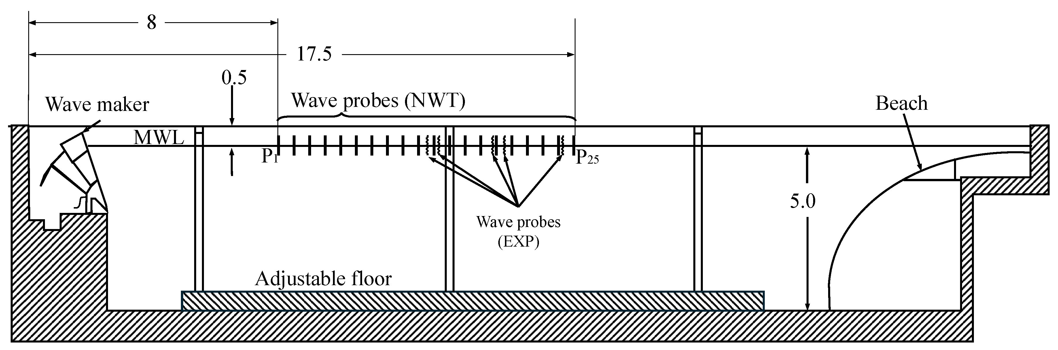
Figure 2.
Short- and long-term data masking to simulate a Monte Carlo dropout of input signals.
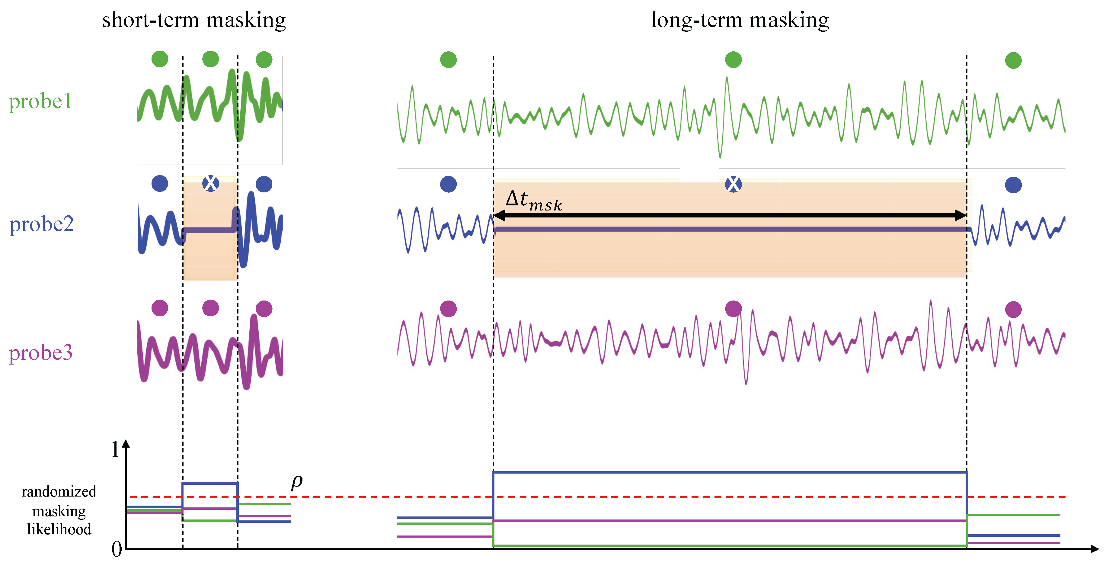
Figure 3.
Phase shift to simulate drift-induced phase changes in floating wave sensor data.
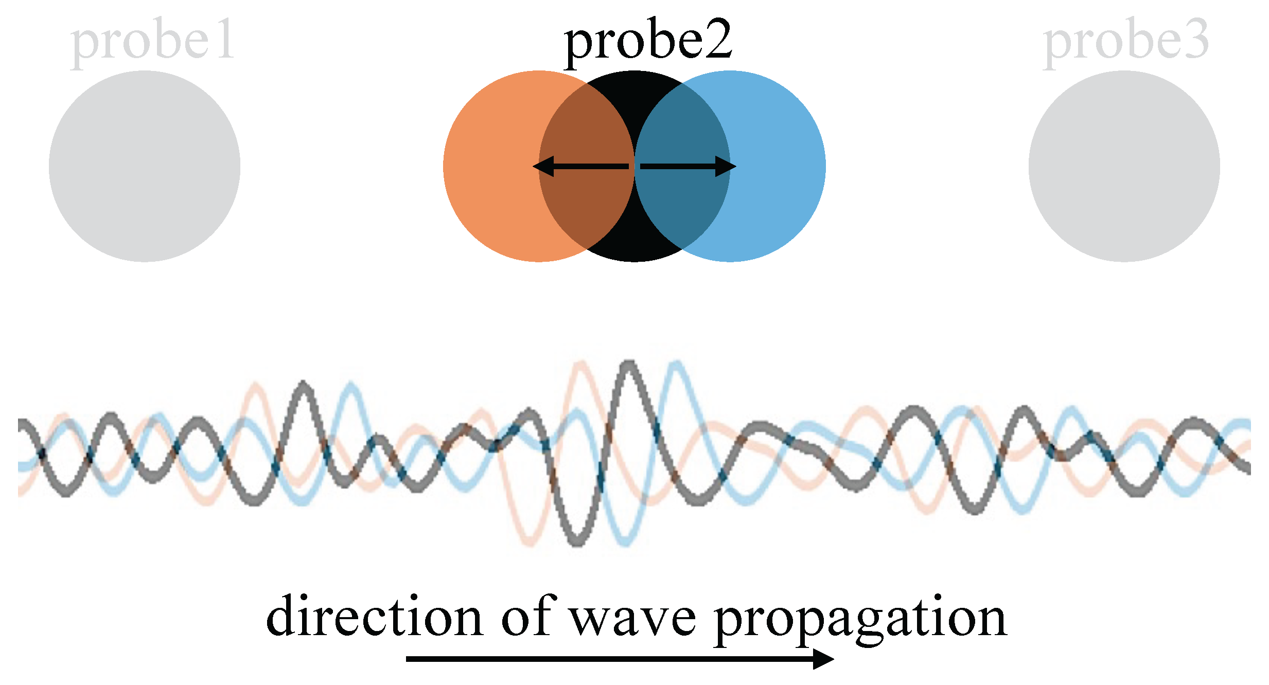
Figure 4.
Development of -trimmed models using uncertainty quantification: (a) Normalized prediction horizon distribution of -trimmed TiDE model for multivariate target, using NWT data. (b) A single stride historical forecast example with uncertainty level curves and their smoothed versions. The vertical dashed lines show -trimmed when uncertainty levels peak over mean threshold.
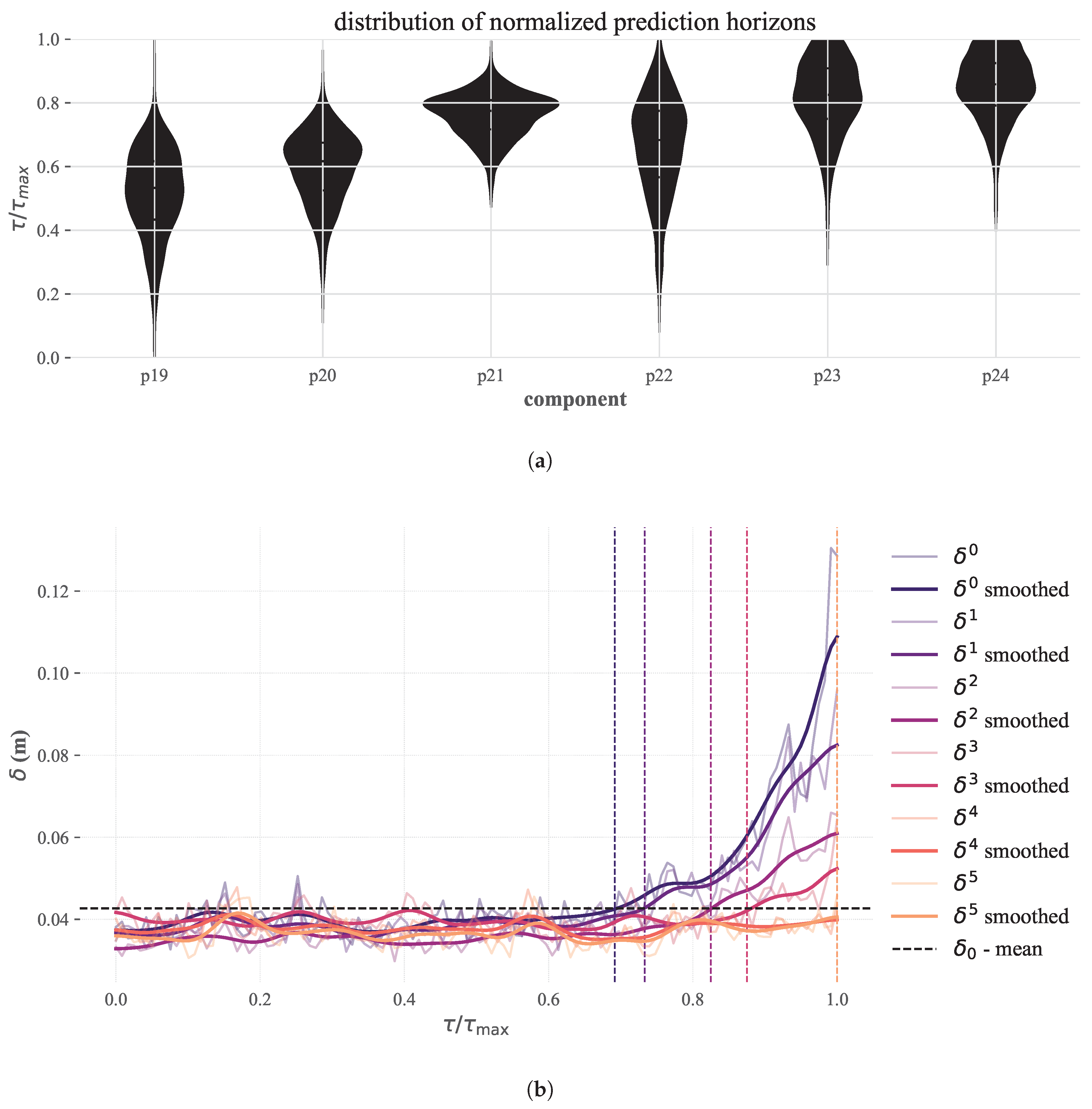
Figure 5.
Prediction error using TiDE models with NWT data for four probability thresholds . (a) Baseline model under short-term masking. (b) -trimmed model under short-term masking. (c) Baseline model under long-term masking. (d) -trimmed model under long-term masking.
Figure 5.
Prediction error using TiDE models with NWT data for four probability thresholds . (a) Baseline model under short-term masking. (b) -trimmed model under short-term masking. (c) Baseline model under long-term masking. (d) -trimmed model under long-term masking.
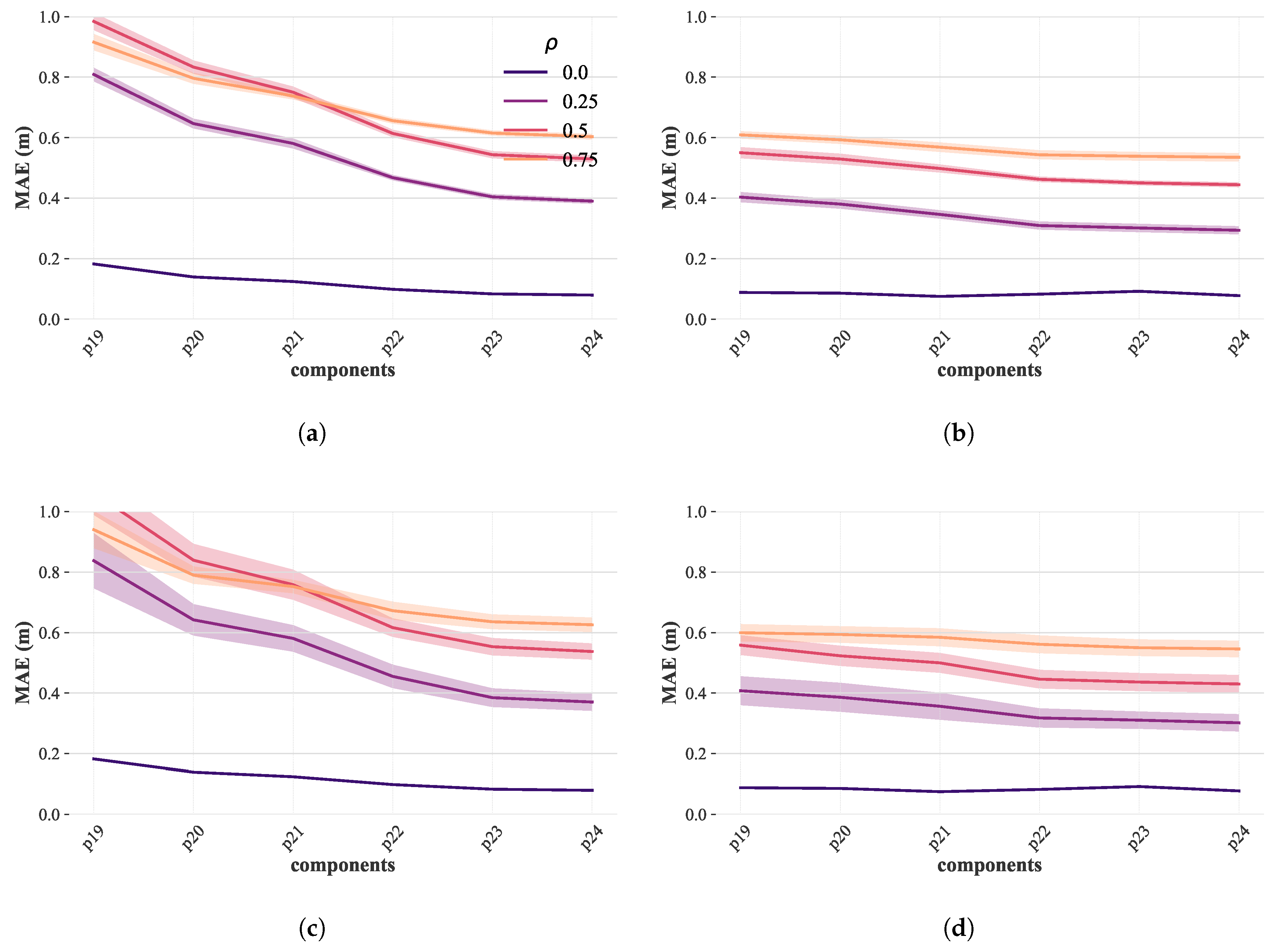
Figure 6.
Prediction error using LSTM models with NWT data for four probability thresholds . (a) Baseline model under short-term masking. (b) -trimmed model under short-term masking. (c) Baseline model under long-term masking. (d) -trimmed model under long-term masking.
Figure 6.
Prediction error using LSTM models with NWT data for four probability thresholds . (a) Baseline model under short-term masking. (b) -trimmed model under short-term masking. (c) Baseline model under long-term masking. (d) -trimmed model under long-term masking.
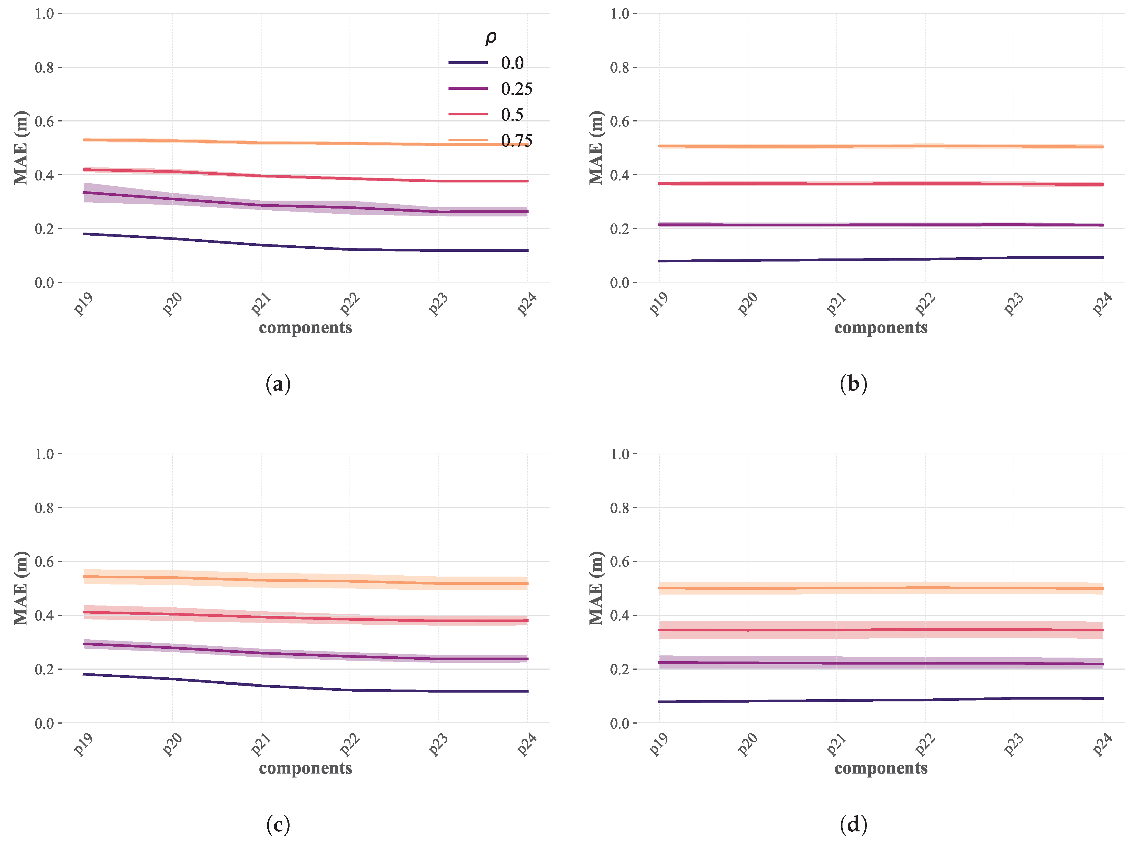
Figure 7.
Normalized prediction horizon distribution of -trimmed models under two sea-state conditions, for experimental data. Horizontal dashed lines represent values for the moderate-type and conservative-type models for each sea-state, superimposed on LWT-based predictable zone shadows. These shadows are computed from minimum and maximum group velocities using upstream probe locations.
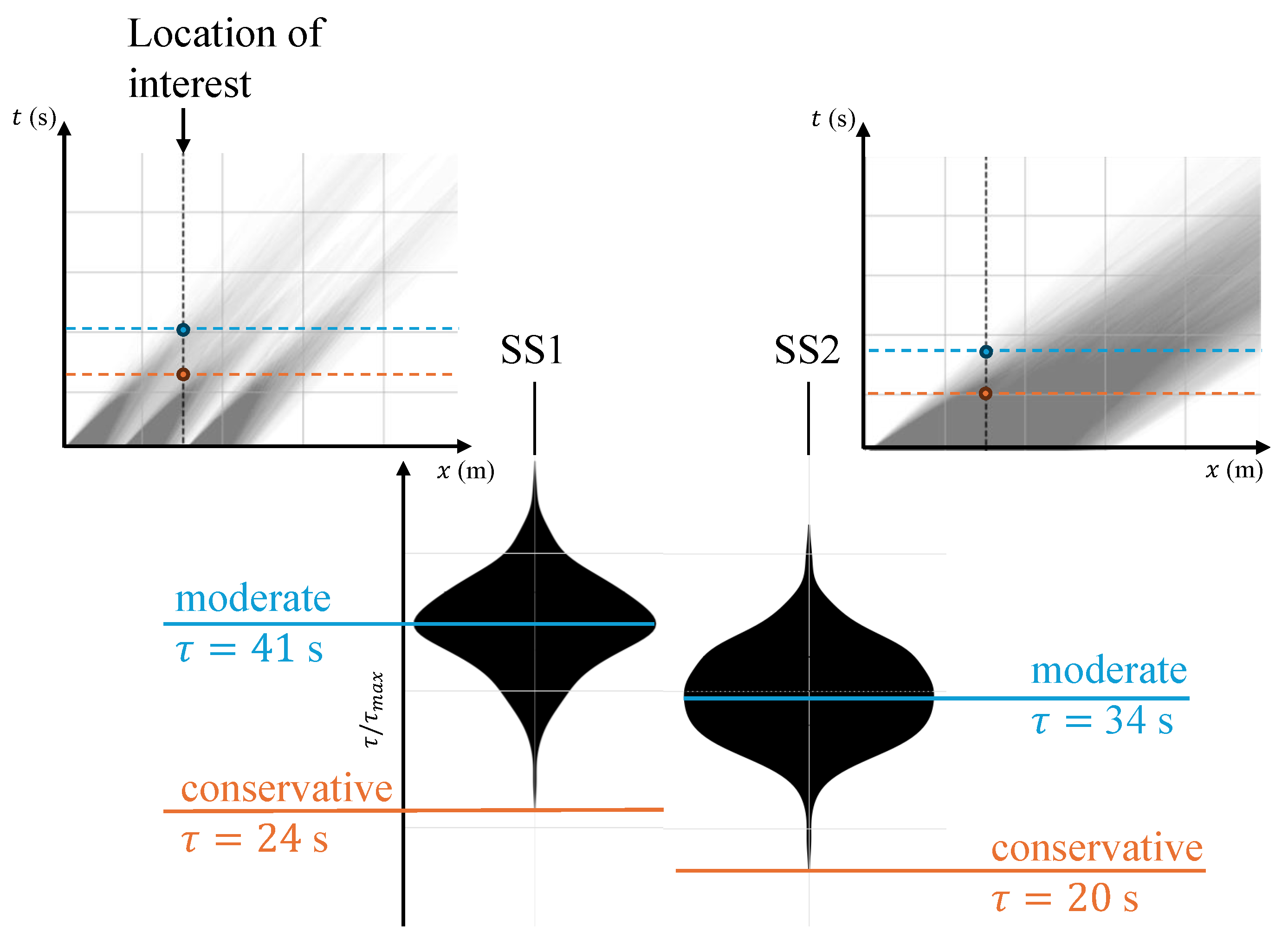
Figure 8.
Impact of short- and long-term data masking on model performance, for experimental data: (a) MAE for moderate and conservative prediction horizons under sea-state SS1. (b) MAE for moderate and conservative prediction horizons under sea-state SS2.
Figure 8.
Impact of short- and long-term data masking on model performance, for experimental data: (a) MAE for moderate and conservative prediction horizons under sea-state SS1. (b) MAE for moderate and conservative prediction horizons under sea-state SS2.
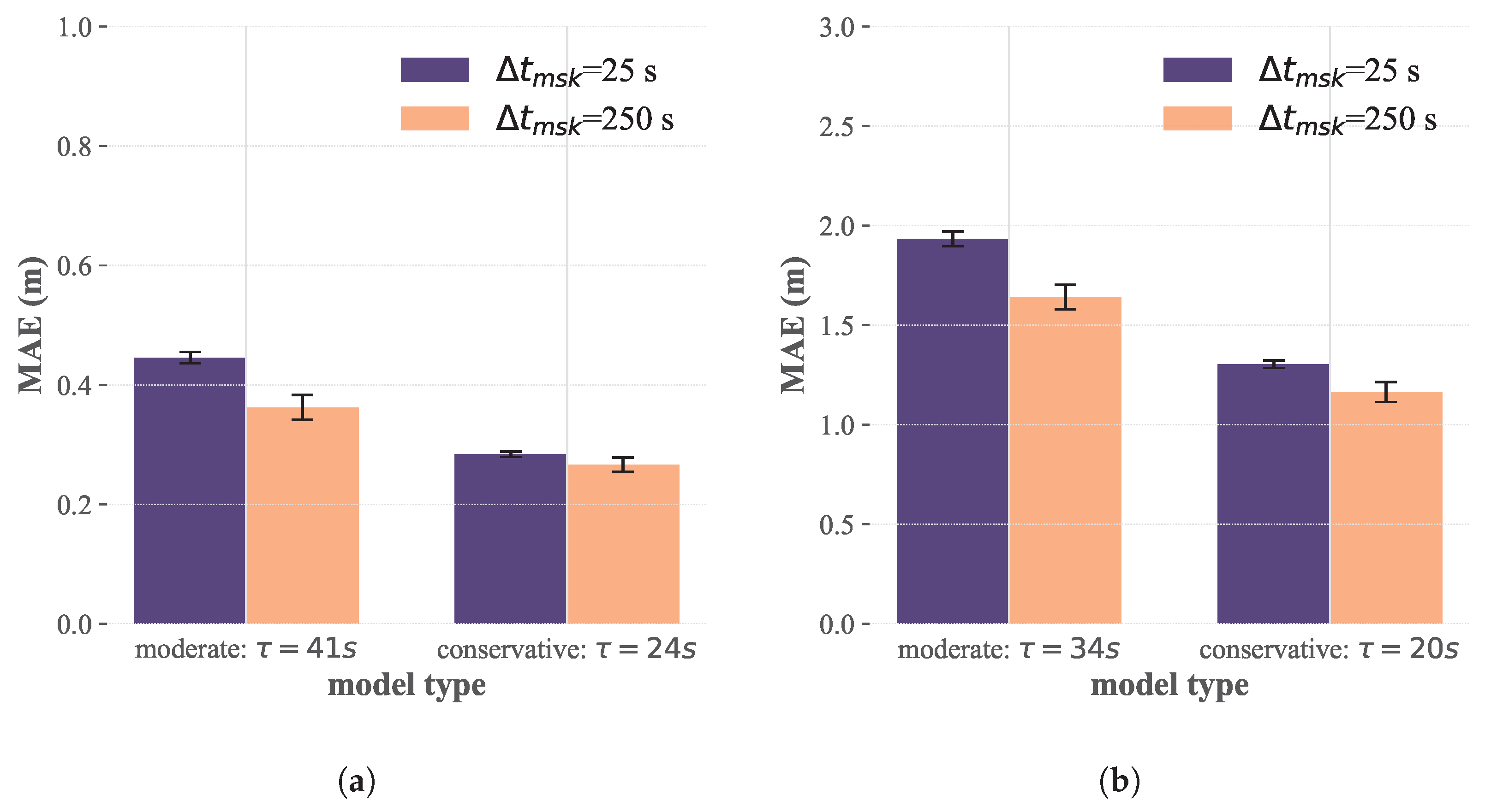
Figure 9.
Instantaneous and smoothed MAE error over time under two conditions, for experimental data: (i) healthy operations with all covariates active, and (ii) loss of the third covariate probe.
Figure 9.
Instantaneous and smoothed MAE error over time under two conditions, for experimental data: (i) healthy operations with all covariates active, and (ii) loss of the third covariate probe.
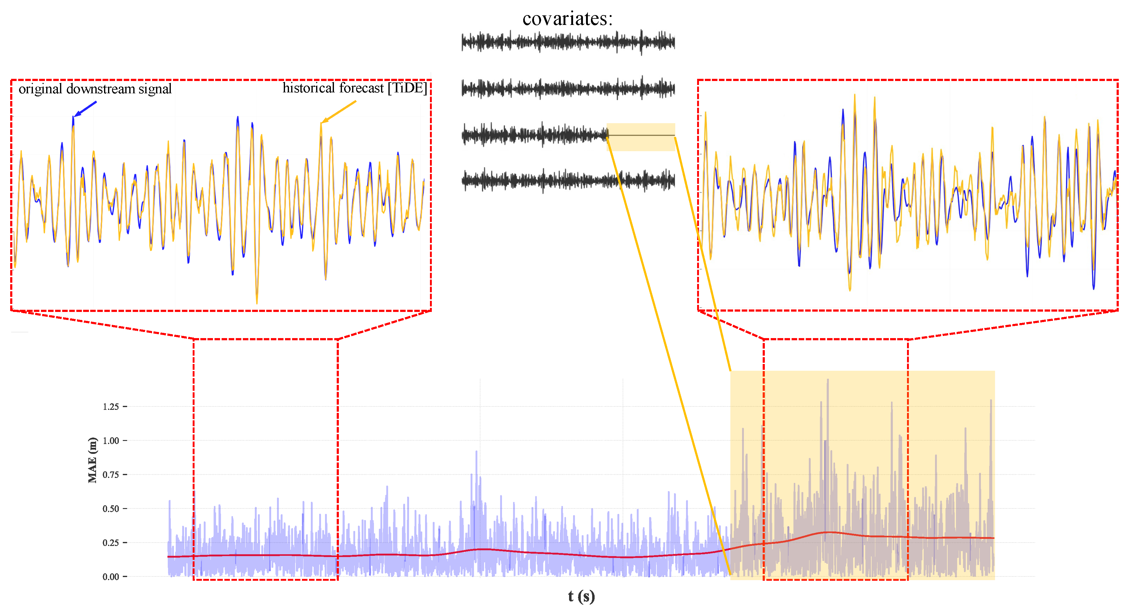
Figure 10.
Impact of phase shift , applied to the first two upstream probes, on model prediction accuracy under experimental conditions: (a) MAE for moderate and conservative prediction horizons under sea-state SS1. (b) MAE for moderate and conservative prediction horizons under sea-state SS2.
Figure 10.
Impact of phase shift , applied to the first two upstream probes, on model prediction accuracy under experimental conditions: (a) MAE for moderate and conservative prediction horizons under sea-state SS1. (b) MAE for moderate and conservative prediction horizons under sea-state SS2.
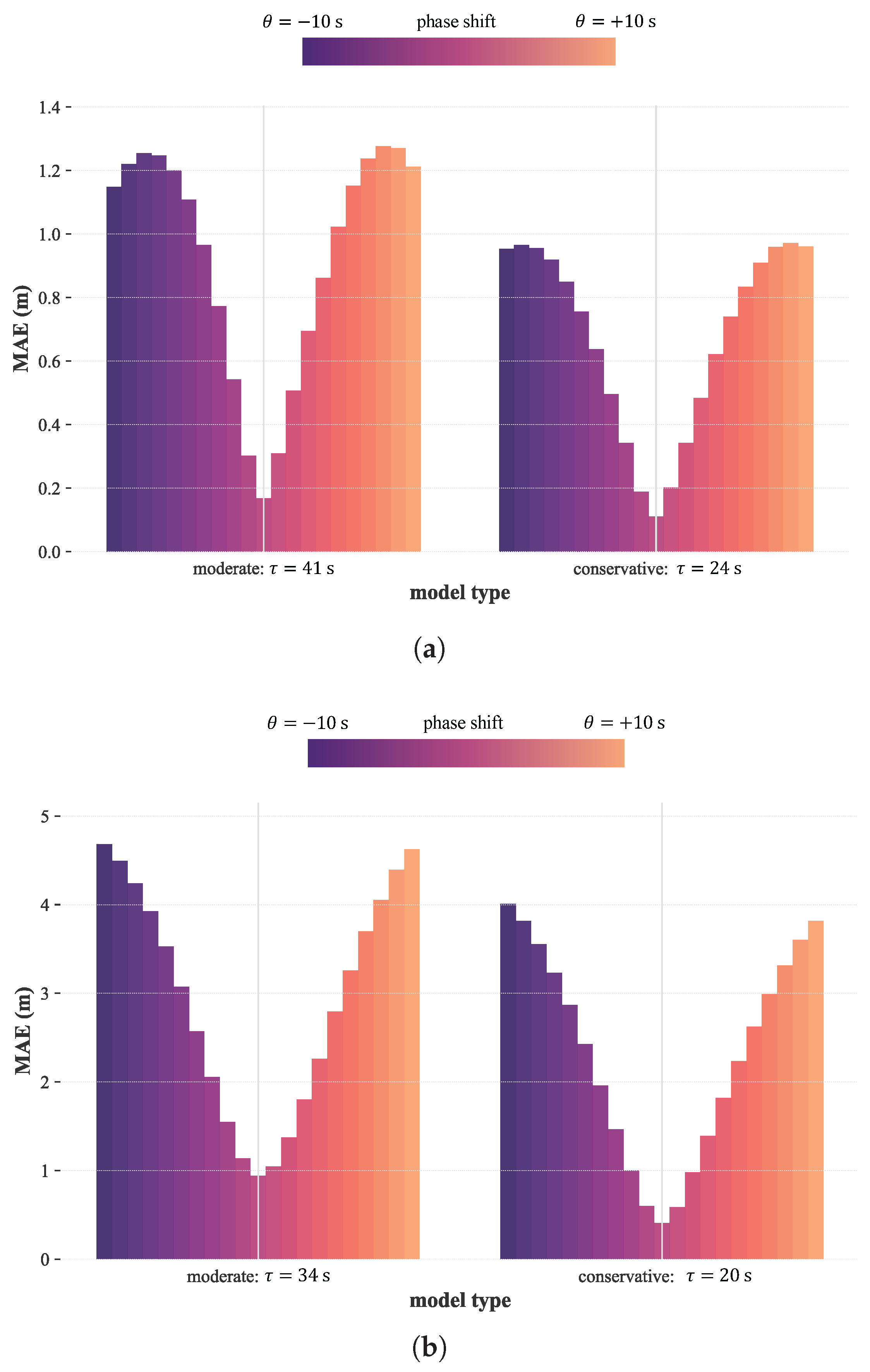

Table 1.
Parameters of two sea-state being investigated.
| Parameters | SS1 | SS2 |
|---|---|---|
| (m) | 3.27 | 10.58 |
| (s) | 9.02 | 14.04 |
| (-) | 1.8 | 2.75 |
Table 2.
Comparison of MAE (m) for baseline and -trimmed TiDE models across different values for probes p19 and p24 (short-term masking), for SS1-related wave data.
Table 2.
Comparison of MAE (m) for baseline and -trimmed TiDE models across different values for probes p19 and p24 (short-term masking), for SS1-related wave data.
| Probe | baseline | -trimmed | diff. | |
|---|---|---|---|---|
| p19 | 0 | 0.182 | 0.088 | -52% |
| 0.25 | 0.828 | 0.417 | -50% | |
| 0.5 | 1.012 | 0.548 | -46% | |
| 0.75 | 0.976 | 0.602 | -38% | |
| p24 | 0 | 0.080 | 0.078 | -2% |
| 0.25 | 0.418 | 0.301 | -28% | |
| 0.5 | 0.546 | 0.429 | -22% | |
| 0.75 | 0.640 | 0.542 | -15% | |
| diff. | 0 | -56% | -12% | |
| 0.25 | -50% | -28% | ||
| 0.5 | -46% | -22% | ||
| 0.75 | -34% | -10% |
Table 3.
Comparison of MAE (m) for baseline and -trimmed LSTM models across different values for probes p19 and p24 (short-term masking), for SS1-related wave data.
Table 3.
Comparison of MAE (m) for baseline and -trimmed LSTM models across different values for probes p19 and p24 (short-term masking), for SS1-related wave data.
| Probe | baseline | -trimmed | diff. | |
|---|---|---|---|---|
| p19 | 0 | 0.181 | 0.080 | -56% |
| 0.25 | 0.291 | 0.217 | -25% | |
| 0.5 | 0.446 | 0.350 | -22% | |
| 0.75 | 0.530 | 0.511 | -4% | |
| p24 | 0 | 0.119 | 0.092 | -23% |
| 0.25 | 0.242 | 0.216 | -11% | |
| 0.5 | 0.402 | 0.344 | -14% | |
| 0.75 | 0.513 | 0.505 | -1% | |
| diff. | 0 | -34% | 15% | |
| 0.25 | -17% | -1% | ||
| 0.5 | -10% | -2% | ||
| 0.75 | -3% | -1% |
Disclaimer/Publisher’s Note: The statements, opinions and data contained in all publications are solely those of the individual author(s) and contributor(s) and not of MDPI and/or the editor(s). MDPI and/or the editor(s) disclaim responsibility for any injury to people or property resulting from any ideas, methods, instructions or products referred to in the content. |
© 2025 by the authors. Licensee MDPI, Basel, Switzerland. This article is an open access article distributed under the terms and conditions of the Creative Commons Attribution (CC BY) license (http://creativecommons.org/licenses/by/4.0/).
Copyright: This open access article is published under a Creative Commons CC BY 4.0 license, which permit the free download, distribution, and reuse, provided that the author and preprint are cited in any reuse.


