
Submitted:
17 October 2023
Posted:
18 October 2023
You are already at the latest version
Abstract
The coastal zone faces an ever-growing risk associated with climate-driven change, including sea level rise and increased frequency of extreme natural hazards. Coastal processes are governed by the dynamic ocean and atmospheric factors with constantly changing conditions. Often the location and dynamism of coastal regions makes them a formidable environment to adequately study with in-situ methods. Remote sensing methods offer an alternative to in-situ monitoring. In this study we use Ice, Cloud, and land Elevation Satellite-2 (ICESat-2) to make measurements of basic wave parameters and wave directionality in the Hawaiian Islands and North Carolina, USA. ICESat-2 has existing Level-3a data products, Ocean Surface Height (ATL12) and Inland Water Elevation (ATL13), providing some wave and ocean surface elevation data. ATL12 provides sparse global average measurements of the sea surface elevation, slope, and roughness along ICESat-2 tracks and ATL13 provides wave metrics at variable length scales out to ~7 km from the coast and does not maintain the 0.7m along-track resolution of the primary Level-2 data product (ATL03). Our goal was to leverage the full resolution data available in ATL03 to generate wave metrics out from shore up to ~25 km. Using a combination of statistical and signal processing methods we can use ICESat-2 to generate basic wave metrics, including significant wave heights with an accuracy of ±0.5m. In some profiles we can identify wave shoaling, which could be used to infer bathymetry. In areas with complex wave dynamics, the nature of how ICESat-2 measures elevations (parallel laser altimetry beams) can make extracting some wave parameters (e.g., wavelength and directionality) more challenging. These wave metrics can provide important data in support of validating wave and tidal models and may also prove useful in ICESat-2 bathymetric corrections and satellite derived bathymetry.
Keywords:
ICESat-2
; coastal waves
; remote sensing of waves
1. Introduction
Coastal regions are the most overt in their response to the changing ocean and are an important lens through which we can view, monitor, and learn about the impacts of climate change on our planet. While representing only ~11% of the Earth’s land surface, coastal regions are home to more than 600 million people [1] and the coastal biome is responsible for 25% of global biological productivity and 80% of known fish species [2]. The coastal ecosystem faces an ever-growing risk associated with climate-driven indicators, including sea level rise and the increased frequency of extreme natural hazards [3]. Coastal processes are governed by the dynamic ocean and atmospheric environments with constantly changing conditions. Understanding how these processes are represented by local water dynamics along the coastline is essential to the prediction of how sea level might threaten the livelihood of coastal communities[4]. However, often the location and dynamism of coastal regions makes them a formidable environment to adequately study with in-situ methods. Buoys can provide some information but are sparsely distributed and often placed in deeper water which precludes measurements that capture the complexities nearer to the shoreline [5]. Similarly, drifters or autonomous surface vehicles (ASV) can also monitor wave motion but the spatial and temporal distribution limit the overall coverage [6,7,8,9]. Space-based observations alleviate some of the complications from field measurements, and even airborne collections give wider spatial coverage, however they can have fairly low temporal latency between repeat passes. Effective instrumentation for satellites focused on ocean surface characterization include radar altimeters, synthetic aperture radar and a multitude of radiometers. These systems have been proven to extract wave heights, ocean heights and ocean vector winds [10,11]. However, the resolution of these systems is often at tens of meters to kilometer spatial scales which leaves large gaps in ocean surface topography and certain nearshore characteristics that vary at short length scales [5,12,13].
In 2018, NASA launched the Ice, Cloud and land Elevation Satellite-2 (ICESat-2), with a state-of-the-art photon counting laser altimeter onboard, poised to provide global height measurements with unprecedented vertical accuracy and precision [14,15]. ICESat-2 provides a way to measure waves at high spatial resolutions ranging from near-shore to the open ocean. Deep water and open ocean waves have been studied using ICESat-2 data [16,17] and ICESat-2 has also been used in coastal zones to extract bathymetry [18,19,20,21,22,23]. ICESat-2 has also proved to be a great resource as supplementary data for other methods like satellite derived bathymetry (SDB), a process that uses spectral band ratios of downwelling irradiance in the water column to estimate a relative depth [24]. The ICESat-2 bathymetric measurements act as ‘seed’ points and can move the image based relative-depth maps to an absolute vertical scale. Other studies in the literature have utilized ICESat-2 as a source of bathymetry training data for SDB which is advantageous to locations that might not have quality ICESat-2 measurement due to clouds or other anomalies [25,26,27,28].
This research seeks to extend the utility of ICESat-2 data for ocean surface characterization in the nearshore environment as a path toward better understanding the dynamics at the land-ocean interface. Our specific research objectives are to: 1) Develop an automated methodology to extract coastal wave metrics including wavelengths/wave period, wave heights (including significant wave heights) from ICESat-2 data, and 2) Explore the possibility of extracting wave directionality from ICESat-2 data. These data have a wide range of uses for validating wave and tidal models, critical data for ICESat-2 bathymetric corrections and satellite derived bathymetry, and possible future ICESat-2 data products.
1.1. ICESat-2
ICESat-2 is a dedicated Earth observing mission borne out of the 2007 National Academies Decadal Survey that prioritized laser altimeter measurements over Earth’s polar regions to monitor changes in the cryosphere. The Level 1 science goals of the mission are focused on quantifying volumetric changes in the ice sheets and sea ice thickness and extent in the Arctic and southern oceans [29]. After a launch in September 2018 the satellite is moving toward 5 years of nominal operation and it completed its prime mission in December of 2021. Onboard the ICESat-2 observatory is the Advanced Topographic Laser Altimetry System (ATLAS) [30]. ATLAS is a photon counting lidar technology that allows for lower laser transmit energy which results in a higher laser repetition rate. These operational aspects of ATLAS create a scenario for higher resolution along-track measurement (0.7 m) and multiple beams (6), both of which mitigate operational constraints identified during the predecessor mission ICESat [31], which operated from 2003 - 2009. The scientific motivation behind the photon counting implementation was to allow the multiple beams to act as a pathway to disentangling surface slope from true elevation change and the high, along-track resolution to reveal small scale feature dynamics, both in the case of repeat measurements.
As many photon-sensitive lidar systems use a Geiger-mode approach, ATLAS employs a linear mode solution with photon-multiplier tubes (PMTs) in the detector focal plane array, not requiring an operational voltage beyond the breakdown level for gain. During the pre-launch phase of the mission, and the core development time of ATLAS, the only available PMTs certified for space environments were operational in the visible spectrum (532 nm). This was a change from the ICESat instrument that used infrared for the surface altimetry measurements as it is better suited to vegetation height retrievals and the laser energy does not penetrate ice- or snow-covered surfaces. Pre-launch efforts established specific surface design cases to optimize the ATLAS performance across a variety of scenarios to satisfy the desire for global surface height measurements [32]. Once on orbit, calibration and validation activities helped in refining aspects contributing to signal level, data quality and repeatability [33]. To date the horizontal accuracy of the measurements is better than 5 m (6.5 m was the mission requirement) [34] and the vertical accuracy is better than 10 cm [14].
ICESat-2’s orbit provides a revisit time of 91-day repeat to the same 1387 reference ground tracks (RGT). In the mid -latitudes, the current operations include an ‘off-pointing’ strategy to densify the coverage along the RGTs and provide more data in between RGTs for the wide range of data products that ICESat-2 supports. Crossing tracks in the opposite orbital direction (ascending vs. descending) and neighboring tracks can provide temporal coverage at ~30 days. As mentioned above, ICESat-2 provides data with six beams in three beam pairs. Each beam pair is separated by ~3.5 km in the across-track direction and consists of a strong and weak beam (a function of the beam splitting optics onboard). The strong and weak beams have an across-track ground separation distance of 90m and an along-track ground separation distance of ~2.5 km.
2. Materials and Methods
2.1. Study Area
For this study we chose three areas that encompass different wave climatologies and different coastal angles/geometry relative to ICESat-2’s orbit (Figure 1). The north shores of the Hawaiian Islands of O’ahu and Kaua’i provided two study areas with shorelines approximately perpendicular to the satellite reference ground tracks. The dominant wave direction at these two sites is from the north and northwest in the winter and northwest to west in the summer. There is a strong seasonality to wave heights with the highest wave heights, 2-4 m, occurring in the winter months and 1-2m in the summer months [35]. The Outer Banks of North Carolina from Kitty Hawk north to Corolla provide a study area with a coastline that is more oblique to ICESat-2’s orbit. North Carolina has overall lower wave heights with 1-2m waves in the winter and 0.5-1 m in the summer. The predominant wave direction for the Outer Banks is from the east with occasional deviations to the north/northeast and south/southeast[35].
For the Kaua’i region, we used one descending ICESat-2 ground track (RGT0282) and one ascending track (RGT1341). For RGT0282 there were five transects with viable data and for RGT1341 two transects with viable data after the preprocessing was completed. O’ahu also had one ascending (RGT1105) and one descending (RGT1219) track, and each had 2 acceptable transects. For North Carolina, we used two ascending tracks (RGT0065 and RGT1368) and one descending track (RGT1010). The ascending tracks both had nine instances of usable data and RGT1010 had four. The other tracks coincident to our study sites were omitted due to cloud cover or other data quality issues associated with satellite maneuvers and orbit adjustments. None of the tracks used were exact geographical repeats due to the mid-latitude pointing strategy of the mission [34] but in near proximity and acceptable for wave dynamic studies. The full list of tracks used is available in the Appendix, Table A1.
2.2. Datasets
The Level 2 data product (ATL03) for ICESat-2 mission is the “Global Geolocated Photons” along-track product and is available through the National Snow and Ice Data Center (NSIDC)[36]. ATL03 provides elevation profiles composed of the individual photon returns. Level 3 along-track mission products use ATL03 to create surface specific elevation profiles that optimize signal finding and length scales most appropriate to the associated science. Two of those Level 3 products are the Ocean Surface Height [ATL12, 37] and Inland Surface Water [ATL13, 38]. ATL12 provides sparse global average measurements of the sea surface elevation, slope, and roughness while ATL13 is designed primarily for inland water bodies and large rivers, but only extends off the coastline ~7 km. However, ATL13 gives elevations at a variable length scale that is related to the signal density (40-80 m) and does not maintain the 0.7m resolution of ATL03, which limits the ability to fully examine the coastal wave metrics.
For the dates and RGTs listed above, we used ATL03 version 005 [36] . Each granule covers approximately 30 degrees of latitude and we geographically subset each granule to extract data in our areas of interest for each study site. During the subsetting process we also removed any individual beam tracks that had missing or insufficient data because of cloud cover or other environmental obscurations.
Our validation data for each site comes from the Wave Watch 3 Global Model (WW3) product available from the Pacific Islands Ocean Observing System (PacIOOS) [39]. For each study site the WW3 data come from a 0.5°x 0.5° model cell (~55 km x 55 km) queried for the date and closest timestamp to the ICESat-2 tracks. The data from the WW3 model includes peak wave direction, peak wave period, significant wave height for the overall wave field, swell component, and wind component. Several tracks overlapped multiple WW3 cells, however we found that the values in adjacent cells did not have large differences and an average value for the cells was used as the comparison value. We calculated additional fields, converting wave period to wavelength and converting wavelength to the ‘apparent wavelength’, the wavelength ICESat-2 should observe based on wave direction. All three of our study sites have buoys in close proximity, however we chose to not use these buoy data for validation since all three sites had significant data gaps that overlapped with several of the ICESat-2 dates that were used in this study.
2.3. ATL03 Preprocessing
To separate the ocean surface from any noise or other features in the photon returns (e.g., clouds or bathymetry), we filtered each beam track in each RGT (6 beams per RGT) using a pseudo-waveform vertical histogramming technique (Figure 2). The pseudo-waveform uses a combination of Gaussian fits for the sea surface and possible sea floor and an exponential fit to model the water column. We adjusted the photon elevation from WGS84 ellipsoidal heights to EGM08 orthometric heights using the geoid parameter in the ATL03 data product. We then used a sliding window of 450 photon returns in the along-track direction to generate a vertical histogram with 5 cm elevation bins. We chose the 450-photon sliding window through an iterative testing of processing with windows from 150 to 1000 photons and performing a qualitative assessment of the surface finding. The 450-photon window gave good surface finding results on both the strong and weak beams while minimizing noise. The point density differences between strong and weak beams and between granules (day vs. night and local atmospheric conditions) make the ground distance covered by each 450-photon window variable. For the strong beam the window size is approximately 100 - 200 m and the weak beam 500-700 m. The most prominent peak in the histogram is taken to be the water surface and the full-width, half-maximum statistic defines whether points are classified as the surface (given a classification value of 1) in each window iteration. Since each 450-photon window overlaps the last window, each photon gets classified 3 times (the window increments 150 photons each iteration) and the average of these classification values represent a confidence score that can be used to eliminate false positives. Only photons with a confidence of 1.0 (classified as surface in each window) are kept. In beam tracks with prominent low clouds or mist/fog that attenuate the laser from reaching the sea surface, the pseudo waveform filter can misclassify these points as sea surface photons. In these cases, we employed a basic interquartile range statistical outlier filter to cull these points that are outside 2.8 of the overall distribution of photo elevations. Over longer distances, ICESat-2 can capture tidal and spatial water surface variations. To exclude those water surface variations from our analysis we applied a simple detrending procedure by subtracting the mean elevation of the beam track from the elevation of each surface photon.
2.4. Basic Wave Metrics
The basic wave metrics we sought to extract were those that match with the data that buoys and the WW3 model generally provide. Significant wave height (Hs) is the average wave height of the largest 33% of waves measured in a period of record or set of observations [40]. Practically, significant wave height can be calculated as a function of the standard deviation of the surface displacement (detrended surface elevations) (1) [40].
Wavelength (L [meters]), wave period (T [seconds]), and wave speed (phase velocity, c [m/s]) are important for understanding the spacing and speed of waves. In analyzing waves with ICESat-2, the measurements for these variables are qualified with “apparent” (e.g., apparent wavelength). This is because the satellite’s orbit inclination of ~92° makes it unlikely that the ground tracks are perpendicular to the travel direction of the waves [17]. When the waves are not traveling perpendicular to the ground track, the wavelengths appear to be elongated by a predictable amount (Apparent Wavelength Factor in Table 1). Frequency spectrum analysis is generally used to extract component frequencies from a set of observations. However, because of the nature of the filtered ICESat-2 photon data we are using, the individual photon returns are not uniformly spaced and there can be significant gaps (from clouds). We chose not to use standard Fourier-base frequency analysis methods that require data sampled at regularly spaced intervals. Instead, we used frequency analysis methods designed for non-uniformly sampled data. To extract the dominant wavelength in each beam track, we used a Lomb-Scargle periodogram [41,42,43] implemented via the AstroPy package [44]. From the resulting periodogram we extracted the wave frequency of the peak spectral power as the dominant wavelength for the track. The frequency units for the periodogram are wave number (k, [cycles/meter]) which are converted to wavelength (2), wave period (3), or phase velocity (4)
where L is wavelength (m), k is wave number (1/m), T is wave period (s), g is the acceleration due to gravity (9.81 m/s2), and c is the phase velocity.
With significant wave height and wavelength, it is also possible to derive the apparent wind speed at z meters above the surface (U(z), Eq. (8)) from the relationship between the roughness length(z0) (5) and the friction velocity (u*) (6)(7) [16,45,46,47]
where z0 is the roughness length, Hs is the significant wave height, L is the apparent wavelength, cp is the dispersion relationship, g is the acceleration due to gravity, u* is the friction velocity, U(z) is the wind at elevation a z elevation above the water surface, k is the von Kármán constant (0.41), and z is the elevation above the water (normally 10 or 15 m).
2.5. Spatial Wave Metrics
In addition to the global wave metrics above, we also wanted to examine spatial patterns in the along-track direction to explore if ICESat-2 can reliably detect shoaling patterns. Shoaling patterns can also be used to infer bathymetry through an inversion of the dispersion relationship. Shoaling of coastal waves is primarily defined by an increase in wave height and decrease in wavelength, since the fundamental frequency is constant [40]. To examine wave height changes, we calculated significant wave heights for the entire beam track for fixed length segments of 0 to 500 m from the coast, 500 to 1000m, and 1000+ m. To find the wavelength changes we employed a wavelet transform method to look at change in wavelength for only the strong beam tracks.
Traditional wavelet transforms have a similar prerequisite to other frequency analysis methods, uniformly sampled data as mentioned above. For our data we used a wavelet transform that handles uneven sampling based on the work of Foster [48] and implemented in Python with the JazzHands Python library [49]. Because our inputs into the wavelet transform were spatial, distance and elevation in meters, the outputs for the transforms were also in spatial frequency units: spatial frequency () in radians/meter, wave number (k) in cycles/meter, wavelength (L) in meters, and the the relationship is . The output of the non-uniform wavelet transformation is two matrices; the weighted wavelet z-transform (WWZ) to locate the wavelet frequencies, and a weighted wavelet amplitude (WWA) to establish the magnitude of the different wavelet frequencies in cells with an along-track resolution of approximately 50 m. For each 50 m cell along-track we find the peak wavelength from the maximum value from the WWA matrix.
2.6. Wave Directionality
The strong/weak beam separation distance of 90 m for each beam pair should allow for the directionality of crests of the detected waves to be determined. The beams are also separated in the along-track direction by ~2.5 km (5 mRad), however because of the spacecraft’s surface equivalent velocity of ~7500 m/s the timing separation between beams is ~0.34 seconds. The spatial difference caused by the along track separation is minimal for waves traveling north/south (along-track), the offset would be 0.34 m for waves traveling at 1 m/s or 1.36 m for waves at 4 m/s. By comparing the waveforms between the strong and weak beams, a spatial offset/lag can be measured between waveforms and the wave travel direction can be calculated as a function of the measured lag using (9) and (10)
where 90 is the strong/weak separation distance, lag distance is waveform offset from a cross correlation analysis, is the ICESat-2 orbital inclination in radians (for ascending tracks , for descending tracks ). Lag distance and are negative when wave angles are 0 - 90° (compass directions) and positive when wave directions are 90 - 180°. Smaller offset distances correspond to waves traveling north/south (crest orientations perpendicular to ICESat-2’s orbit) and larger offsets correspond to waves traveling east/west (crest orientations more parallel with ICESat-2’s orbit) (see theoretical offset distances in Table 1 and Figure 3). Because each ICESat-2 overpass is an instantaneous snapshot of the waves crest direction can only be determined in 180° compass angle pairs (e.g., 0-180° or 45-225°) and the actual wave travel direction can be inferred by the dominant regional wave patterns in relation to the coast (i.e., waves generally travel from open water toward the coast). The main assumption in determining directionality is that the strong and weak beams must have very clear waveforms in the photon returns and those detected waves are coherent/in-phase to allow for comparison. In the near-coastal environment, there are also several factors that could impact coherence of the wave signals and the ability to measure directionality; velocity variation due to bathymetry, wave refraction by coastal features, wave reflections from the coast, and constructive or destructive interference. We chose to approach this problem from both a theoretical perspective, with simulated waves, and a practical perspective, with actual data.
For the simulated waves, we generated several 3-dimensional wave fields over an area of 2 km by 2 km. Each simulated wavefield was created using a sine wave with constant wavelengths between 40-300 m and an amplitude of 1 m with added Gaussian noise to the elevation to simulate ICESat-2 surface returns. To simulate waves from different compass directions, we rotated the wave field and extracted points from the wave fields using two profiles inclined at 92° and separated by 90 m to mimic ICESat-2’s orbit and beam separation. The extracted surface points were then resampled to a regular along track interval using a rolling median filter (window size = 2 m) and a Piecewise Cubic Hermite Interpolating Polynomial (PCHIP). The analysis of ICESat-2 data follows the same resampling workflow.
To calculate the wave direction in both the simulated data and ICESat-2 data we used a cross-correlation technique (Scipy’s signal.correlate and signal.correlation_lags)[50] to evaluate the waveforms in each beam track. The output of the cross correlation is a matrix with discrete linear cross-correlation values and the corresponding lag distances. The lag distance with the highest cross correlation value was taken as the offset for (9) and (10).
3. Results
3.1. Wave Height
Measurements of significant wave heights compared favorably to the WW3 modeled wave heights with a mean error of 0.07 m ( and minimum and maximum of 0.58 m (Figure 4). At smaller wave heights (<1 m), the ICESat-2 measurements tend to overestimate the wave heights (ICESat-2 > WW3). While significant wave heights >1 m, can be over- or under estimated compared to the WW3 model.
3.2. Wavelength
From the Lomb-Scargle frequency analysis of each track we interpreted the frequency with the highest spectral power as the dominant wavelength in the track. A direct comparison to the WW3 model values shows a significant amount of error (Figure 5a), because we are comparing the apparent wavelengths from ICESat-2 with the “true” WW3 wavelengths of waves coming from a variety of directions. To make these values comparable we calculated what the apparent wavelength would be from the WW3 data based on ICESat-2’s orbit and the relationship explained above. In Figure 5b, the comparison of apparent wavelengths, the spread of the errors is very large, however in the range of 0-500 m the correspondence between ICESat-2 and WW3 is closer to the 1:1 line. Beyond 1000 m apparent wavelengths, the errors are considerably larger. These results suggest that that the overall peak frequency metric from a Lomb-Scargle analysis might be oversimplifying the actual patterns and may not be the best metric for trying to extract wavelengths from ICESat-2 data.
3.3. Wavelets
For the wavelet analysis, we focused on only the strong beam tracks. Because of the sparse data density in the weak beams, the wavelet outputs were extremely noisy and tended to favor the extreme longer wavelengths. Overall, the non-uniform wavelet analyses were able to extract the spatial patterns of wavelengths along each track. In Figure 6, the surface photon returns are shown (top) and the corresponding wavelet plots (bottom) illustrate the wavelet amplitude for each wavelength (y-axis) for 50-meter segments away from shore (x-axis). In both surface return plots, there is a clear decrease in wavelengths closer to the shore and the same decrease can be seen in the wavelet plots.
The wavelet plot for Oahu (Figure 6d) also illustrates one of the issues that did arise in this analysis. The mis-calculation of wavelengths because of the nature of the surface return data. From 4 to 5.5 km offshore, the peak wavelet power jumps from a wavelength of 350 m at 4 km from shore to a 1200 m wavelength at 4.25 km until 5.5 km offshore. In the surface return data from 4 - 5.5 km, the wavelength shift is caused by a broad parabolic pattern with some shorter wavelength periodicity. The parabolic pattern dominates the frequency spectrum for this length of the track and artificially inflates the wavelengths.
3.4. Directionality
By simulating wave fields at different wavelengths and sampling them at known wave angles we were able to determine that there is a minimum wavelength necessary in order to calculate all possible compass directions. When the theoretical offset distance (Table 1) for any given wave angle exceeds the wavelength, the cross-correlation lag parameters default to the shortest distance to achieve the maximum correlation. These shorter distances are not directly relatable to the wave angles and cause significant errors in the calculated angles (Figure 3b). For shorter wavelengths, it is possible to accurately calculate directions where the wavelength is less than the theoretical lag distance, however to calculate all possible wave directions the wavelengths must be greater than 180 m.
For the Kauai and Oahu sites, the dominant wave directions in the wave climatologies are from the north, therefore the wave angles should be calculable for a wide range of wavelengths. For the North Carolina site, the dominant wave directions are from the northeast and east, which would require longer wavelengths to calculate the full range of wave directions. Figure 7 illustrates an example of cross correlation for Oahu (RGT1219-GT3, 2022-MAR-12). The Lomb-Scargle wavelengths were calculated at 666 m for the strong beam and 665 m for the weak beam (WW3 model apparent wavelength = 591 m). The peak cross correlation lag distance in Figure 7b is -114 m which corresponds to a wave angle of 130.29/310.29°. From the WW3 model data, the overall wave direction was 304° and the swell direction was 308.5°. The difference on the overall wave direction is 6.29° and the difference on the swell direction is 1.79°.
In Figure 8, the histograms of cross correlation direction for all tracks illustrates significant spread in the results for this method. When comparing the calculated angle to the overall wave direction in the WW3 data (Figure 8a), this method correctly predicts the wave direction at +/-10 degrees for 21% of the tracks and +/- 20 degrees for 30% of the tracks. Compared to the WW3 Swell direction (Figure 8b), our method correctly predicts +/-10 degrees for 19% of the tracks and +/- 20 degrees for 41% of the tracks.
We also split each track into smaller segments (0-5 km from shore, 5-10 km, 10-15 km) (Figure 8c-e) to see if there was any influence of distance from the shore affecting the distance calculations (e.g., move complex waveforms affecting the cross correlations) and to test if smaller segments of the overall waveform would produce different results. All three distance groups perform similarly, with no significant difference between them.
4. Discussion
4.1. Basic Wave Metrics
The accuracy of the significant wave heights match with similar analyses in previous studies using ICESat-2 in the open ocean that reported errors in the range of ±0.5m [16,17]. Our results also compare well to those produced by studies comparing Sentinel-1 data to WW3. Kahn et al. [51] reported mean significant wave height errors of 0.15 – 0.32m (RMSE 0.64 – 0.76m) and Wang et al. [52] had mean wave height errors of 0.21 – 0.32m (RMSE 0.5-0.64). The sources of error in significant wave height are likely the result of incorrectly classified surface points affecting the standard deviation of elevation calculation. In both strong and weak beams, there are often photon returns that are close to the water surface that are either in the air or water column that are classified as surface points. Because of their proximity to actual surface points, they are difficult to filter out without affecting the overall surface classification.
Wavelength measurements in coastal settings with ICESat-2 are complicated by both the wave direction and the physical interactions of different types of waves. While the results presented here do have considerable errors; the study by Yu et al. [17] in an open ocean setting comparing to WW3 data also showed a considerable range of error in their wavelength calculation ranging across +/-450 m with a mean difference of 57m and an RMSE of 151m. Our results suggest that there are other wave interactions happening that affect the wavelength spectra and calculations. As mentioned above, the apparent wavelength that ICESat-2 observes is a function of the wave direction, with no little difference between apparent and actual wavelengths at 0/180° and stretching the wavelengths by 117% at 30/210°, 213% at 60/250°, and 444% at 75/255°. Wave refraction near/around shore features and around whole islands in the case of our Hawaiian sites can create waveforms that are compressed and stretched differentially based on their interaction with the shoreline. Wave reflections from the shore can also impact the calculated wave spectra through constructive and destructive interference. The overall interactions between swell and wind waves can also affect the wave spectral that ICESat-2 measures. Wind waves impart a higher frequency/shorter wavelength onto the overall signal, however, depending on the strength and direction of the local wind compared to the overall swell direction the influence of the wind can create a complicated overall waveform. Figure 9 illustrates some of these interactions as seen from the Sentinel-1 synthetic aperture radar satellite image around O’ahu and demonstrates how spatially variable the wave patterns can be. In Figure 9b, the coastal detail image, the main swell pattern can be seen coming from the northwest, reflected waves are visible at the coast, and the interaction of wind from the east can be seen on the surface. In the overview panel (Figure 9a), the spatial extent of the local wind patterns can also be observed in the “wind shadows” on the west facing coastlines of the island.
One of ICESat-2’s advantages is that it collects nearly-instantaneous elevation profiles by traveling at a surface equivalent velocity of ~7500 m/s. This can also be a disadvantage compared to most physical measurement techniques (e.g., buoys) and numeric models that use smoothing techniques and temporal averages to ameliorate the noise inherent in measuring a dynamic sea surface. The wave structure that ICESat-2 captures is a discrete snapshot of the surface elevation and can therefore have structure, like the parabolic structure affecting Figure 6d, that may or may not be representative of the overall signal.
4.2. Wavelets
The wavelet analysis of ICESat-2 tracks is advantageous over the Lomb-Scargle method because it can extract the along-track spatial patterns of wavelengths rather than just the overall wave spectra. The spatial patterns of wavelength are important because wave characteristics can change rapidly in the coastal zone. The rapid change in wave parameters in the coastal zone can be indicative of shoaling, as waves interact with the seafloor and wavelengths decrease and wave heights increase. Shoaling characteristics are evident in many of the ICESat-2 tracks (ex. Figure 6a @ ~2 km and Figure 7c @ ~1 km), but not all tracks. Since shoaling is a function of a combination of factors such as wave height, wavelength, wave direction, depth, and seabed slope, certain combinations of these parameters could create larger differences in the breaking waves that ICESat-2 can measure or smaller differences that may not be visible in the ICESat-2 data. Where shoaling is clear, with the addition of local estimates of wave height, it would be possible to use ICESat-2 data as part of a bathymetry inversion to estimate the bathymetry based on the wave and shoaling patterns [23,53,54]. Similar to the overall wavelength calculations, the complicated waveforms that ICESat-2 captures can have an adverse effect on the wavelet analysis.
4.3. Directionality
The key underlying assumption for calculating wave direction from ICESat-2 is that the waves are coherent/in-phase between the strong and weak beams. In the simulated data, this is an easy variable to control and the patterns of wavelength and direction are clear, including the challenges associated with measuring the direction at shorter wavelengths. Based on our results, when calculating directionality, most coastal ICESat-2 tracks are likely violating the coherent assumption. This is likely one of the biggest sources of error and a key limitation in attempting to calculate wave directionality from ICESat-2. All the complexities of the wave field already discussed are amplified since the directionality calculations are essentially extending two 1-dimensional elevation profiles into a 3-dimensional analysis space with an unknown sea state in the 90-meter gap between the strong and weak beams. The errors we are seeing are not unlike those reported for open sea conditions by Yu et al. [17], who used more tracks than were presented here but had a range of errors that extended to +/- 90°. Because of the broad spatial coverage provided by radar and imaging satellite sensors like Sentinel-1, directionality is more straightforward. Khan et al. [51] were able to calculate wave direction with mean errors of ~3° (RMSE ~30°).
Another limitation in making the directionality calculations is the weak beam density. The decreased density of photon returns can adversely affect the creation of the waveform for the cross-correlation and potentially affect some of the other metrics as well. In this research, the weak beams densities for the water surface returns were on average 39% of the strong beam, which is similar to results over forested landscapes [55] and in-line with the original design specifications for ICESat-2 [32]. This power point density difference can lead to waveforms that can be too smooth or potentially at different frequencies than the strong beam. When possible, we recommend using the strong beams for most wave parameter extraction operations.
5. Conclusions
We have demonstrated that ICESat-2 can be used for extracting basic wave metrics in the near-coastal zone and that the results are similar to similar ICESat-2 studies done in the open ocean. ICESat-2 can provide significant wave heights with a mean error of 0.7 m. These wave metrics can provide important data in support of validating wave and tidal models as well as for using ICESat-2 bathymetric corrections and satellite derived bathymetry. There are limitations when using ICESat-2 to measure wavelengths and wave directionality related to the way that ICESat-2 measures elevations as near instantaneous elevation profiles. Wavelength measurements are influenced by the direction of travel of the wave relative to ICESat-2’s orbit and directionality is dependent on the correlation of the wave surface profiles between strong and weak beams. More research is needed on these two topics which may include employing or developing more robust techniques for handling missing data along the tracks and handling the data density differences between the strong and weak beams. Adding ancillary data, such as buoy data, wave models (e.g., WW3), or other earth observations satellite data, would be another way to improve a wave processing workflow that would complement ICESat-2 data and potentially create a more robust dataset for wave analysis. These data and future improvements to ICESat-2 derived wave metrics have a wide range of uses for validating wave and tidal models, critical data for ICESat-2 bathymetric corrections and satellite derived bathymetry, and possible future ICESat-2 data products.
Author Contributions
Conceptualization, JTD and LAM; methodology, JTD.; software, JTD and MH; validation, JTD; formal analysis, JTD; investigation, JTD; writing—original draft preparation, JTD; writing—review and editing, LAM and MH; project administration, LAM; funding acquisition, LAM. All authors have read and agreed to the published version of the manuscript.
Funding
Funding for this research was provided through a NASA grant 80NSSC22K1878 from the ICESat-2 Project Science Office at Goddard Space Flight Center in Greenbelt, MD for the development of an along-track bathymetry product and through NASA grant 80NSSC22K1102 for the Decadal Survey Incubation program focus on Surface, Topography and Vegetation Science Team.
Data Availability Statement
The ICESat-2 ATL03 data used in this study are available via the National Snow and Ice Data Center (NSIDC) - nsidc.org [36].
Acknowledgments
The authors would like to acknowledge the helpful comments and discussions with Jonathan Markel and Christopher Parrish. We would also like to thank the four anonymous reviewers for their comments that helped improve this paper.
Conflicts of Interest
The authors declare no conflict of interest. The funders had no role in the design of the study; in the collection, analyses, or interpretation of data; in the writing of the manuscript; or in the decision to publish the results.
Appendix A

Table A1.
Dates, Reference Ground Tracks, and beams for the ICESat-2 data used in this study.
| O'ahu | Kaua'i | North Carolina | ||||||
|---|---|---|---|---|---|---|---|---|
| Date | RGT | Beams | Date | RGT | Beams | Date | RGT | Beams |
| 2020-Dec-5 | 1105 | 1,2,3 | 2018-Oct-17 | 282 | 1,2,3 | 2019-Oct-1 | 65 | 1,2,3 |
| 2022-Mar-4 | 1105 | 1,2,3 | 2019-Oct-15 | 282 | 1,2,3 | 2020-Jun-29 | 65 | 1,2,3 |
| 2022-Sep-2 | 1105 | 1,2,3 | 2021-Jan-11 | 282 | 1,2,3 | 2020-Dec-28 | 65 | 1,2 |
| 2019-Sep-15 | 1219 | 1 | 2021-Apr-12 | 282 | 1,2,3 | 2021-Jun-27 | 65 | 1,2,3 |
| 2020-Dec-13 | 1219 | 1,2,3 | 2022-Oct-9 | 282 | 1,2,3 | 2021-Sep-26 | 65 | 1,2,3 |
| 2022-Mar-12 | 1219 | 1,2,3 | 2021-Jun-20 | 1341 | 1,2,3 | 2021-Dec-26 | 65 | 1,2,3 |
| 2022-Sep-17 | 1341 | 1,2,3 | 2022-Mar-27 | 65 | 1,2,3 | |||
| 2022-Jun-26 | 65 | 1,2,3 | ||||||
| 2022-Sep-24 | 65 | 1,2,3 | ||||||
| 2020-Mar-1 | 1010 | 2,3 | ||||||
| 2020-Nov-29 | 1010 | 1,2,3 | ||||||
| 2021-Feb-28 | 1010 | 1,2,3 | ||||||
| 2021-Nov-27 | 1010 | 1,2,3 | ||||||
| 2018-Dec-27 | 1368 | 1,2,3 | ||||||
| 2019-Mar-28 | 1368 | 1,2,3 | ||||||
| 2019-Sep-25 | 1368 | 1,2,3 | ||||||
| 2019-Dec-25 | 1368 | 1,2,3 | ||||||
| 2020-Jun-24 | 1368 | 1,2,3 | ||||||
| 2020-Sep-22 | 1368 | 1,2,3 | ||||||
| 2020-Dec-22 | 1368 | 1,2,3 | ||||||
| 2021-Jun-22 | 1368 | 1,2,3 | ||||||
| 2022-Mar-21 | 1368 | 1,2,3 | ||||||
| 2022-Sep-19 | 1368 | 1,2,3 |
References
- Hauer, M.E.; Fussell, E.; Mueller, V.; Burkett, M.; Call, M.; Abel, K.; McLeman, R.; Wrathall, D. Sea-Level Rise and Human Migration. Nat Rev Earth Environ 2020, 1, 28–39. [CrossRef]
- Vandeweerd, V.; Bernal, P.; Belfiore, S.; Goldstein, K.; Cicin-Sain, B. A Guide to Oceans, Coasts, and Islands at the World Summit on Sustainable Development.; Center for the Study of Marine Policy, 2002.
- Manes, S.; Gama-Maia, D.; Vaz, S.; Pires, A.P.F.; Tardin, R.H.; Maricato, G.; Bezerra, D. da S.; Vale, M.M. Nature as a Solution for Shoreline Protection against Coastal Risks Associated with Ongoing Sea-Level Rise. Ocean & Coastal Management 2023, 235, 106487. [CrossRef]
- Vousdoukas, M.I.; Mentaschi, L.; Voukouvalas, E.; Verlaan, M.; Jevrejeva, S.; Jackson, L.P.; Feyen, L. Global Probabilistic Projections of Extreme Sea Levels Show Intensification of Coastal Flood Hazard. Nat Commun 2018, 9, 2360. [CrossRef]
- Ardhuin, F.; Stopa, J.E.; Chapron, B.; Collard, F.; Husson, R.; Jensen, R.E.; Johannessen, J.; Mouche, A.; Passaro, M.; Quartly, G.D.; et al. Observing Sea States. Frontiers in Marine Science 2019, 6.
- Centurioni, L.; Braasch, L.; Lauro, E.D.; Contestabile, P.; Leo, F.D.; Casotti, R.; Franco, L.; Vicinanza, D. A NEW STRATEGIC WAVE MEASUREMENT STATION OFF NAPLES PORT MAIN BREAKWATER. Coastal Engineering Proceedings 2016, 36–36. [CrossRef]
- Li, M.; Zhang, S.; Qi, Z.; Dang, C. Application of Wave Drifter to Marine Environment Observation. In Proceedings of the OCEANS 2016 - Shanghai; April 2016; pp. 1–5.
- Lumpkin, R.; Özgökmen, T.; Centurioni, L. Advances in the Application of Surface Drifters. Annual Review of Marine Science 2017, 9, 59–81. [CrossRef]
- Pearman, D.W.; Herbers, T.H.C.; Janssen, T.T.; van Ettinger, H.D.; McIntyre, S.A.; Jessen, P.F. Drifter Observations of the Effects of Shoals and Tidal-Currents on Wave Evolution in San Francisco Bight. Continental Shelf Research 2014, 91, 109–119. [CrossRef]
- Figa-Saldaña, J.; Wilson, J.J.W.; Attema, E.; Gelsthorpe, R.; Drinkwater, M.R.; Stoffelen, A. The Advanced Scatterometer (ASCAT) on the Meteorological Operational (MetOp) Platform: A Follow on for European Wind Scatterometers. Canadian Journal of Remote Sensing 2002, 28, 404–412. [CrossRef]
- Wang, H.; Mouche, A.; Husson, R.; Chapron, B.; Yang, J.; Liu, J.; Ren, L. Quantifying Uncertainties in the Partitioned Swell Heights Observed From CFOSAT SWIM and Sentinel-1 SAR via Triple Collocation. IEEE Transactions on Geoscience and Remote Sensing 2022, 60, 1–16. [CrossRef]
- Hauser, D.; Abdalla, S.; Ardhuin, F.; Bidlot, J.-R.; Bourassa, M.; Cotton, D.; Gommenginger, C.; Evers-King, H.; Johnsen, H.; Knaff, J.; et al. Satellite Remote Sensing of Surface Winds, Waves, and Currents: Where Are We Now? Surv Geophys 2023. [CrossRef]
- Villas Bôas, A.B.; Ardhuin, F.; Ayet, A.; Bourassa, M.A.; Brandt, P.; Chapron, B.; Cornuelle, B.D.; Farrar, J.T.; Fewings, M.R.; Fox-Kemper, B.; et al. Integrated Observations of Global Surface Winds, Currents, and Waves: Requirements and Challenges for the Next Decade. Frontiers in Marine Science 2019, 6.
- Brunt, K.M.; Neumann, T.A.; Smith, B.E. Assessment of ICESat-2 Ice Sheet Surface Heights, Based on Comparisons Over the Interior of the Antarctic Ice Sheet. Geophysical Research Letters 2019, 46, 13072–13078. [CrossRef]
- Brunt, K.M.; Neumann, T.A.; Larsen, C.F. Assessment of Altimetry Using Ground-Based GPS Data from the 88S Traverse, Antarctica, in Support of ICESat-2. The Cryosphere 2019, 13, 579–590. [CrossRef]
- Klotz, B.W.; Neuenschwander, A.; Magruder, L.A. High-Resolution Ocean Wave and Wind Characteristics Determined by the ICESat-2 Land Surface Algorithm. Geophysical Research Letters 2020, 47, e2019GL085907. [CrossRef]
- Yu, Y.; Sandwell, D.T.; Gille, S.T.; Villas Bôas, A.B. Assessment of ICESat-2 for the Recovery of Ocean Topography. Geophysical Journal International 2021, 226, 456–467. [CrossRef]
- Cao, B.; Fang, Y.; Gao, L.; Hu, H.; Jiang, Z.; Sun, B.; Lou, L. An Active-Passive Fusion Strategy and Accuracy Evaluation for Shallow Water Bathymetry Based on ICESat-2 ATLAS Laser Point Cloud and Satellite Remote Sensing Imagery. International Journal of Remote Sensing 2021, 42, 2783–2806. [CrossRef]
- Chen, Y.; Chen, Y.; Zhu, Z.; Le, Y.; Qiu, Z.; Chen, G.; Wang, L.; Wang, L. Refraction Correction and Coordinate Displacement Compensation in Nearshore Bathymetry Using ICESat-2 Lidar Data and Remote-Sensing Images. Opt. Express, OE 2021, 29, 2411–2430. [CrossRef]
- Leng, Z.; Zhang, J.; Ma, Y.; Zhang, J.; Zhu, H. A Novel Bathymetry Signal Photon Extraction Algorithm for Photon-Counting LiDAR Based on Adaptive Elliptical Neighborhood. International Journal of Applied Earth Observation and Geoinformation 2022, 115, 103080. [CrossRef]
- Parrish, C.E.; Magruder, L.A.; Neuenschwander, A.L.; Forfinski-Sarkozi, N.; Alonzo, M.; Jasinski, M. Validation of ICESat-2 ATLAS Bathymetry and Analysis of ATLAS’s Bathymetric Mapping Performance. Remote Sensing 2019, 11, 1634. [CrossRef]
- Ranndal, H.; Sigaard Christiansen, P.; Kliving, P.; Baltazar Andersen, O.; Nielsen, K. Evaluation of a Statistical Approach for Extracting Shallow Water Bathymetry Signals from ICESat-2 ATL03 Photon Data. Remote Sensing 2021, 13, 3548. [CrossRef]
- Yang, J.; Ma, Y.; Zheng, H.; Xu, N.; Zhu, K.; Wang, X.H.; Li, S. Derived Depths in Opaque Waters Using ICESat-2 Photon-Counting Lidar. Geophysical Research Letters 2022, 49, e2022GL100509. [CrossRef]
- Stumpf, R.P.; Holderied, K.; Sinclair, M. Determination of Water Depth with High-Resolution Satellite Imagery over Variable Bottom Types. Limnology and Oceanography 2003, 48, 547–556. [CrossRef]
- Albright, A.; Glennie, C. Nearshore Bathymetry From Fusion of Sentinel-2 and ICESat-2 Observations. IEEE Geoscience and Remote Sensing Letters 2021, 18, 900–904. [CrossRef]
- Babbel, B.J.; Parrish, C.E.; Magruder, L.A. ICESat-2 Elevation Retrievals in Support of Satellite-Derived Bathymetry for Global Science Applications. Geophysical Research Letters 2021, 48, e2020GL090629. [CrossRef]
- Ma, Y.; Xu, N.; Liu, Z.; Yang, B.; Yang, F.; Wang, X.H.; Li, S. Satellite-Derived Bathymetry Using the ICESat-2 Lidar and Sentinel-2 Imagery Datasets. Remote Sensing of Environment 2020, 250, 112047. [CrossRef]
- Thomas, N.; Lee, B.; Coutts, O.; Bunting, P.; Lagomasino, D.; Fatoyinbo, L. A Purely Spaceborne Open Source Approach for Regional Bathymetry Mapping. IEEE Transactions on Geoscience and Remote Sensing 2022, 60, 1–9. [CrossRef]
- Markus, T.; Neumann, T.; Martino, A.; Abdalati, W.; Brunt, K.; Csatho, B.; Farrell, S.; Fricker, H.; Gardner, A.; Harding, D.; et al. The Ice, Cloud, and Land Elevation Satellite-2 (ICESat-2): Science Requirements, Concept, and Implementation. Remote Sensing of Environment 2017, 190, 260–273. [CrossRef]
- Martino, A.J.; Neumann, T.A.; Kurtz, N.T.; McLennan, D. ICESat-2 Mission Overview and Early Performance. In Proceedings of the Sensors, Systems, and Next-Generation Satellites XXIII; SPIE, October 10 2019; Vol. 11151, pp. 68–77.
- Schutz, B.E.; Zwally, H.J.; Shuman, C.A.; Hancock, D.; DiMarzio, J.P. Overview of the ICESat Mission. Geophysical Research Letters 2005, 32. [CrossRef]
- Neumann, T.A.; Martino, A.J.; Markus, T.; Bae, S.; Bock, M.R.; Brenner, A.C.; Brunt, K.M.; Cavanaugh, J.; Fernandes, S.T.; Hancock, D.W.; et al. The Ice, Cloud, and Land Elevation Satellite – 2 Mission: A Global Geolocated Photon Product Derived from the Advanced Topographic Laser Altimeter System. Remote Sensing of Environment 2019, 233, 111325. [CrossRef]
- Luthcke, S.B.; Thomas, T.C.; Pennington, T.A.; Rebold, T.W.; Nicholas, J.B.; Rowlands, D.D.; Gardner, A.S.; Bae, S. ICESat-2 Pointing Calibration and Geolocation Performance. Earth and Space Science 2021, 8, e2020EA001494. [CrossRef]
- Magruder, L.; Brunt, K.; Neumann, T.; Klotz, B.; Alonzo, M. Passive Ground-Based Optical Techniques for Monitoring the On-Orbit ICESat-2 Altimeter Geolocation and Footprint Diameter. Earth and Space Science 2021, 8, e2020EA001414. [CrossRef]
- Scripps Institution of Oceanography Coastal Data Information Program Buoy Data Available online: https://cdip.ucsd.edu/ (accessed on 12 May 2023).
- Neumann, T.A.; Brenner, A.; Hancock, D.; Robbins, J.; Saba, J.; Harbeck, K.; Gibbons, A.; Lee, J.; Luthcke, S.B.; Rebold, T. ATLAS/ICESat-2 L2A Global Geolocated Photon Data, Version 5 2021.
- Morison, J.H.; Hancock, D.; Dickinson, S.; Robbins, J.; Roberts, L.; Kwok, R.; Palm, S.P.; Smith, B.; Jasinski, M.F.; ICESat-2 Science Team ATLAS/ICESat-2 L3A Ocean Surface Height, Version 5 2022.
- Jasinski, M.F.; Stoll, J.D.; Hancock, D.; Robbins, J.; Nattala, J.; Morison, J.; Jones, B.M.; Ondrusek, M.E.; Pavelsky, T.M.; Parrish, C.; et al. ATLAS/ICESat-2 L3A Along Track Inland Surface Water Data, Version 5 2021.
- Cheung, K.F. WaveWatch III (WW3) Global Wave Model 2023.
- Stewart, R.H. Introduction to Physical Oceanography; Robert H. Stewart, 2008.
- Lomb, N.R. Least-Squares Frequency Analysis of Unequally Spaced Data. Astrophys Space Sci 1976, 39, 447–462. [CrossRef]
- Scargle, J.D. Studies in Astronomical Time Series Analysis. II. Statistical Aspects of Spectral Analysis of Unevenly Spaced Data. The Astrophysical Journal 1982, 263, 835–853. [CrossRef]
- VanderPlas, J.T. Understanding the Lomb–Scargle Periodogram. ApJS 2018, 236, 16. [CrossRef]
- The Astropy Collaboration; Price-Whelan, A.M.; Lim, P.L.; Earl, N.; Starkman, N.; Bradley, L.; Shupe, D.L.; Patil, A.A.; Corrales, L.; Brasseur, C.E.; et al. The Astropy Project: Sustaining and Growing a Community-Oriented Open-Source Project and the Latest Major Release (v5.0) of the Core Package*. ApJ 2022, 935, 167. [CrossRef]
- Drennan, W.M.; Graber, H.C.; Hauser, D.; Quentin, C. On the Wave Age Dependence of Wind Stress over Pure Wind Seas. Journal of Geophysical Research: Oceans 2003, 108. [CrossRef]
- Drennan, W.M.; Taylor, P.K.; Yelland, M.J. Parameterizing the Sea Surface Roughness. Journal of Physical Oceanography 2005, 35, 835–848. [CrossRef]
- Taylor, P.K.; Yelland, M.J. The Dependence of Sea Surface Roughness on the Height and Steepness of the Waves. Journal of Physical Oceanography 2001, 31, 572–590. [CrossRef]
- Foster, G. Wavelets for Period Analysis of Unevenly Sampled Time Series. The Astronomical Journal 1996, 112, 1709. [CrossRef]
- Dorn-Wallenstein, T.; Desai, A.; Gilbert, G.; RT, A.; Monsue, T. JazzHands 2020.
- Virtanen, P.; Gommers, R.; Oliphant, T.E.; Haberland, M.; Reddy, T.; Cournapeau, D.; Burovski, E.; Peterson, P.; Weckesser, W.; Bright, J.; et al. SciPy 1.0: Fundamental Algorithms for Scientific Computing in Python. Nature Methods 2020, 17, 261–272. [CrossRef]
- Khan, S.S.; Echevarria, E.R.; Hemer, M.A. Ocean Swell Comparisons Between Sentinel-1 and WAVEWATCH III Around Australia. Journal of Geophysical Research: Oceans 2021, 126, e2020JC016265. [CrossRef]
- Wang, H.; Mouche, A.; Husson, R.; Grouazel, A.; Chapron, B.; Yang, J. Assessment of Ocean Swell Height Observations from Sentinel-1A/B Wave Mode against Buoy In Situ and Modeling Hindcasts. Remote Sensing 2022, 14, 862. [CrossRef]
- Santos, D.; Abreu, T.; Silva, P.A.; Baptista, P. Estimation of Coastal Bathymetry Using Wavelets. Journal of Marine Science and Engineering 2020, 8, 772. [CrossRef]
- Santos, D.; Fernández-Fernández, S.; Abreu, T.; Silva, P.A.; Baptista, P. Retrieval of Nearshore Bathymetry from Sentinel-1 SAR Data in High Energetic Wave Coasts: The Portuguese Case Study. Remote Sensing Applications: Society and Environment 2022, 25, 100674. [CrossRef]
- Neuenschwander, A.; Magruder, L.; Guenther, E.; Hancock, S.; Purslow, M. Radiometric Assessment of ICESat-2 over Vegetated Surfaces. Remote Sensing 2022, 14, 787. [CrossRef]
Figure 1.
Study areas showing areas of interest and ICESat-2 ground tracks. Background imagery from MAXAR/DigitalGlobe.
Figure 1.
Study areas showing areas of interest and ICESat-2 ground tracks. Background imagery from MAXAR/DigitalGlobe.
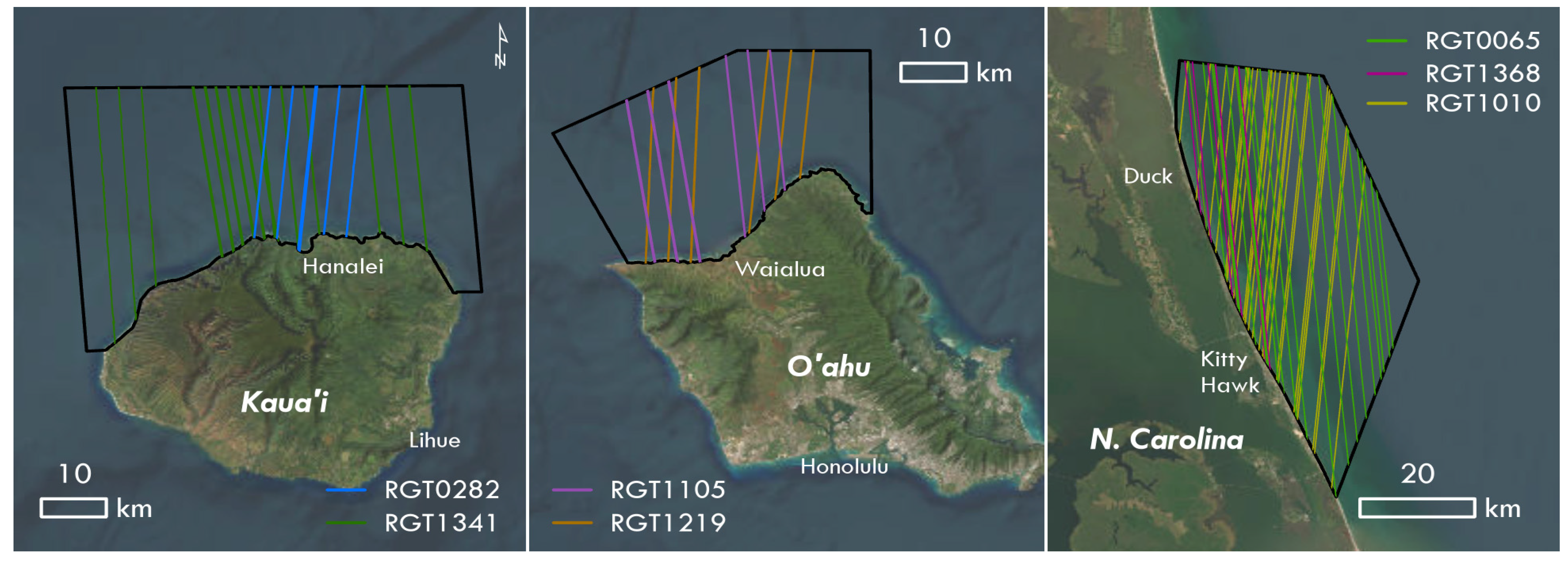
Figure 2.
An example profile classification for Kaua'i. (a) Raw ATL03 photo data and (b) classified photon data using pseudo-waveform methods.
Figure 2.
An example profile classification for Kaua'i. (a) Raw ATL03 photo data and (b) classified photon data using pseudo-waveform methods.
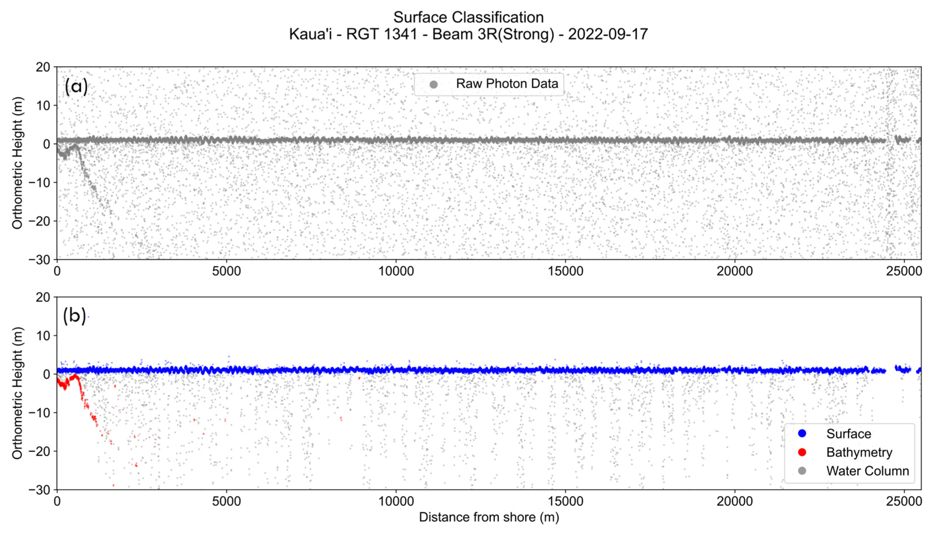
Figure 3.
(a) Illustration of wave directionality angles used in Eq. 10. (b) Illustration of the problem on measuring shorter wavelengths, where in shorter wavelength cases the angle measurements in (a) are complicated by overlapping wave crests interfering with the trigonometric calculations.
Figure 3.
(a) Illustration of wave directionality angles used in Eq. 10. (b) Illustration of the problem on measuring shorter wavelengths, where in shorter wavelength cases the angle measurements in (a) are complicated by overlapping wave crests interfering with the trigonometric calculations.
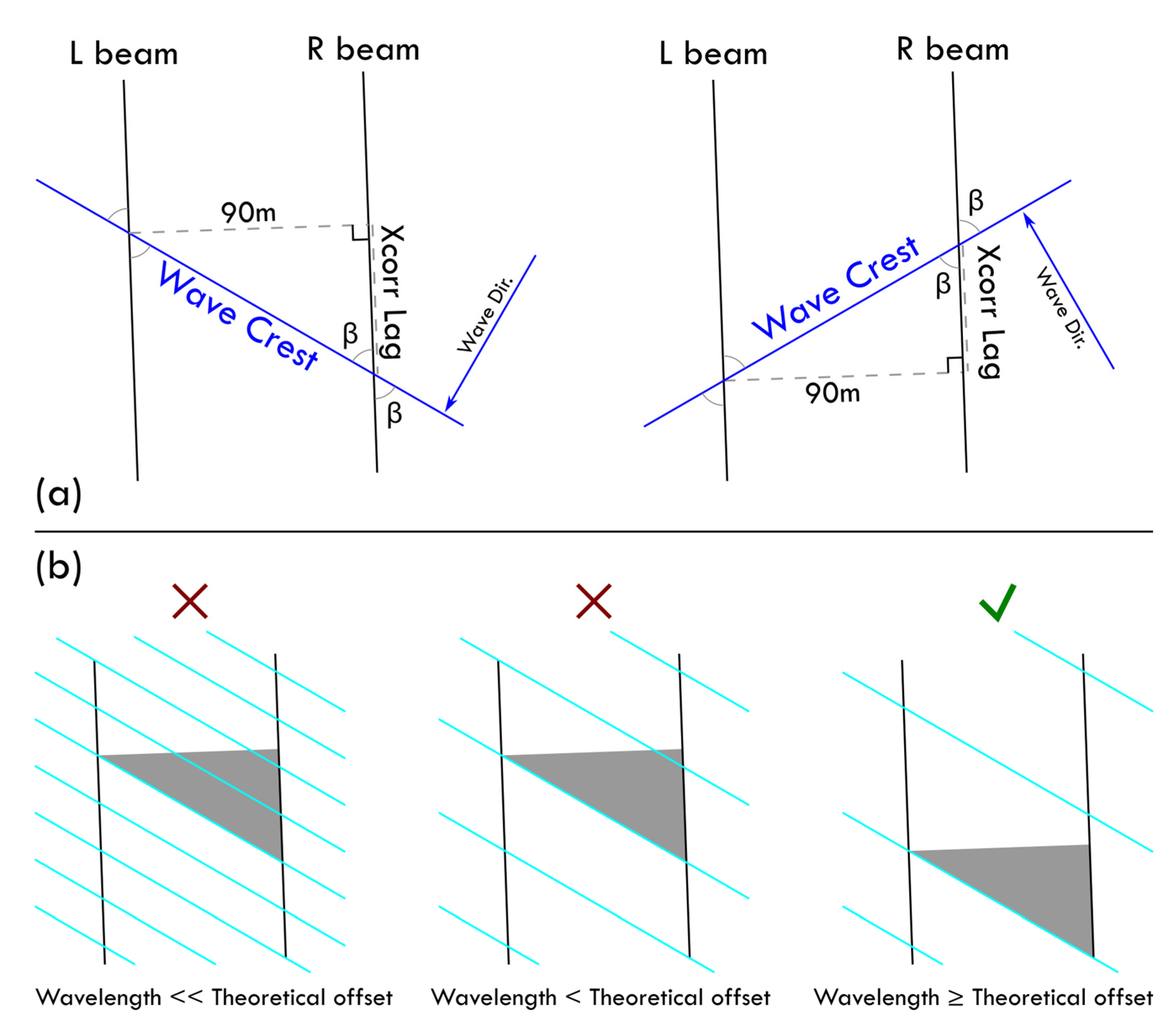
Figure 4.
Significant wave height results compared to WW3 model values. (a) Scatter plot of significant wave heights measured by ICESat-2 and modelled by WW3, linear regression is for strong and weak combined. (b) Histogram of the differences between ICESat-2 and WW3 significant wave heights.
Figure 4.
Significant wave height results compared to WW3 model values. (a) Scatter plot of significant wave heights measured by ICESat-2 and modelled by WW3, linear regression is for strong and weak combined. (b) Histogram of the differences between ICESat-2 and WW3 significant wave heights.
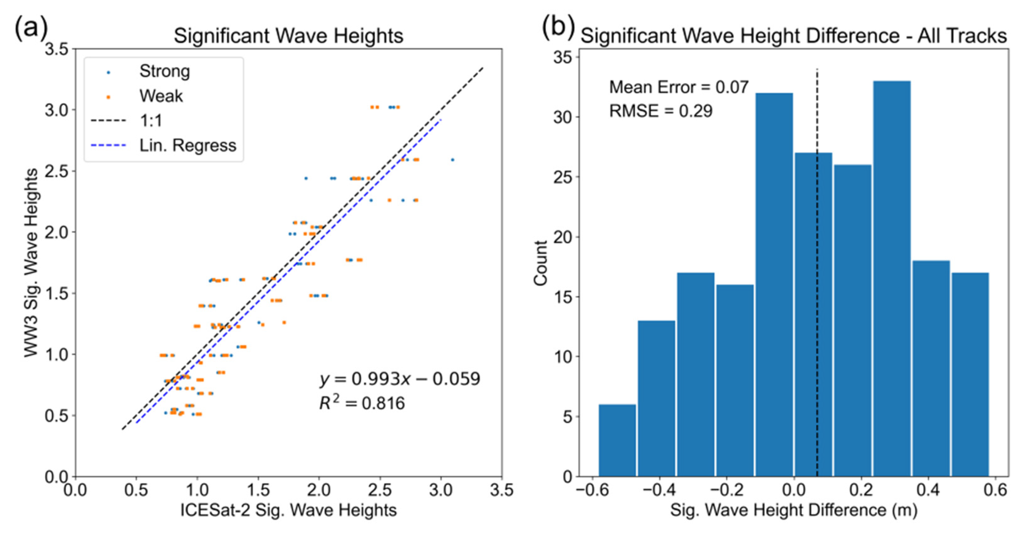
Figure 5.
Wavelength results. (a) Scatterplot of peak wavelengths calculated for ICESat-2 vs. WW3 peak wavelengths. (b) Scatterplot of peak wavelengths calculated for ICESat-2 vs. apparent WW3 peak wavelengths (adjusted by WW3 wave direction to account for ICESat-2’s orbital inclination). (c) Boxplots showing the distribution of wavelength differences in (a, Real) and (b, Apparent).
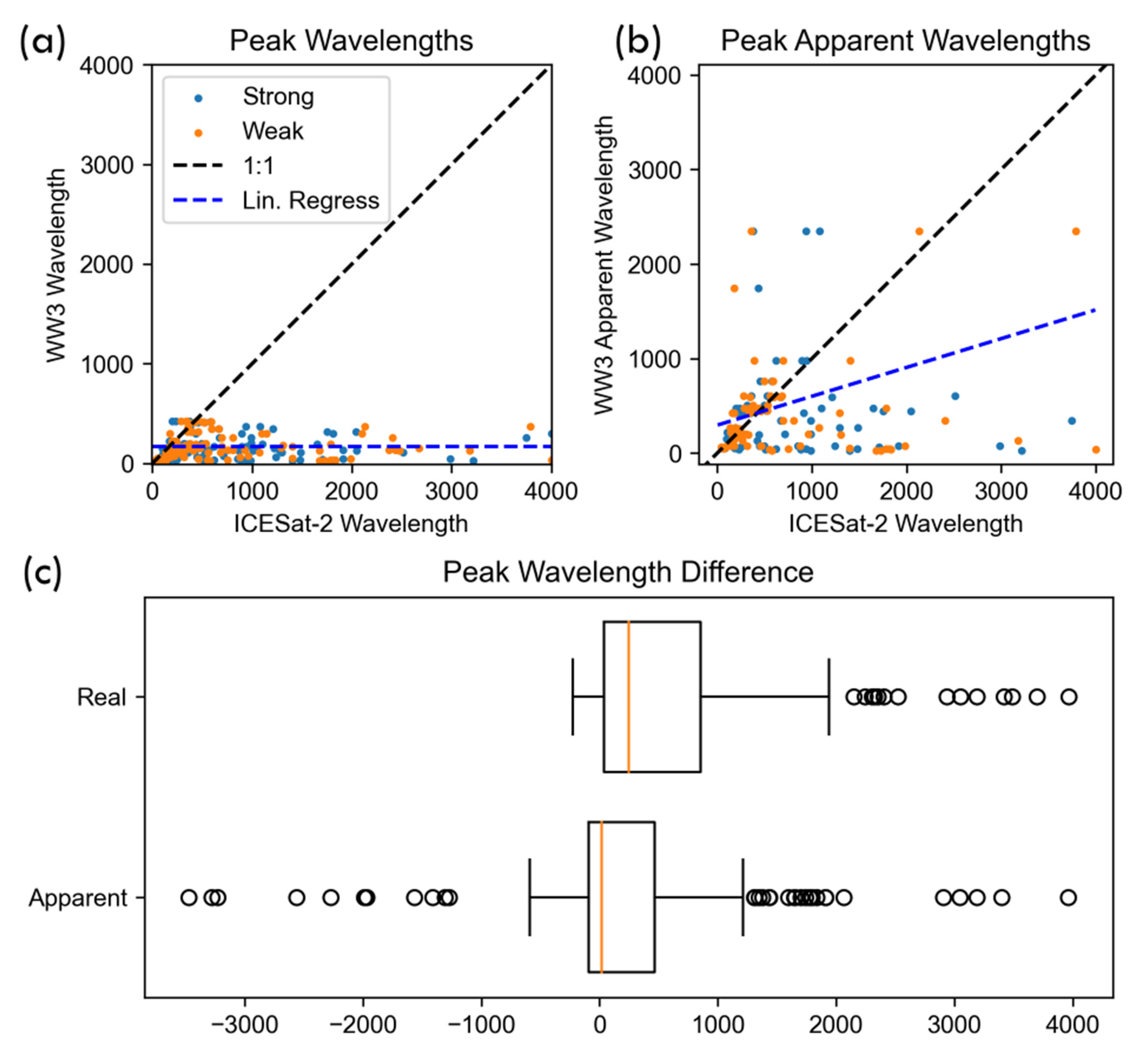
Figure 6.
(a and c) Photon surface return profiles and (b and d) corresponding weighted wavelet amplitude (WWA) plots. The black line in the wavelet plots traces the peak wavelength in each along-track cell of the wavelet analysis.
Figure 6.
(a and c) Photon surface return profiles and (b and d) corresponding weighted wavelet amplitude (WWA) plots. The black line in the wavelet plots traces the peak wavelength in each along-track cell of the wavelet analysis.
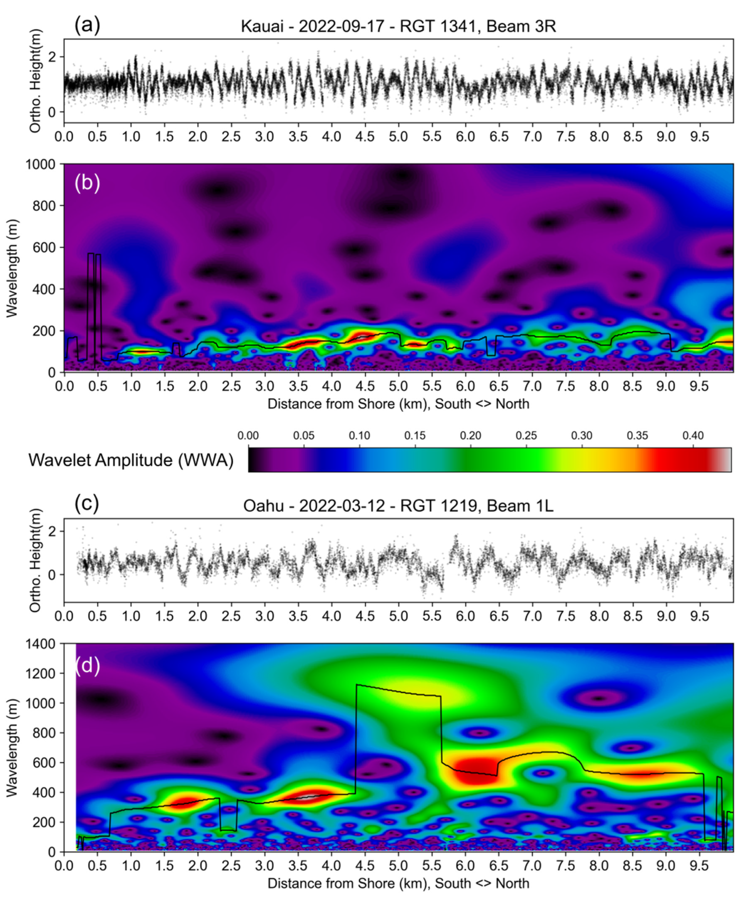
Figure 7.
(a) Interpolated surface profiles for the strong and weak beams for RGT1219 on 2022-March-12. (b) Cross-correlation results comparing the profiles in (a).
Figure 7.
(a) Interpolated surface profiles for the strong and weak beams for RGT1219 on 2022-March-12. (b) Cross-correlation results comparing the profiles in (a).
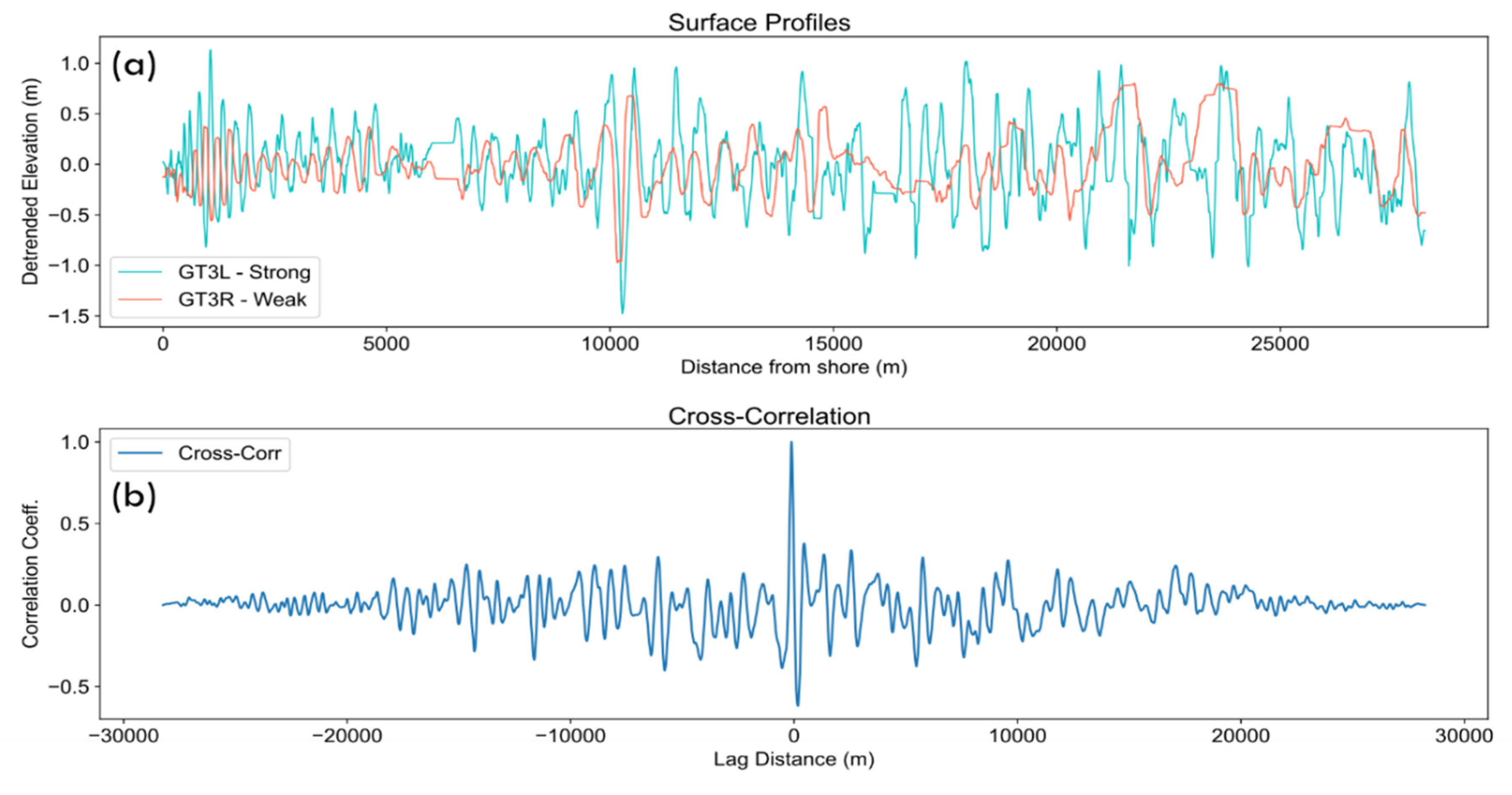
Figure 8.
Histograms showing the absolute differences between the calculated wave direction and WW3 wave direction. (a) Differences between calculated wave direction for full tracks and overall WW3 wave direction. (b) Differences between calculated wave direction for full tracks and swell WW3 wave direction. (c-e) Differences between calculated wave direction for 0-5, 5-10, and 10-15 kilometers from shore and overall WW3 wave direction.
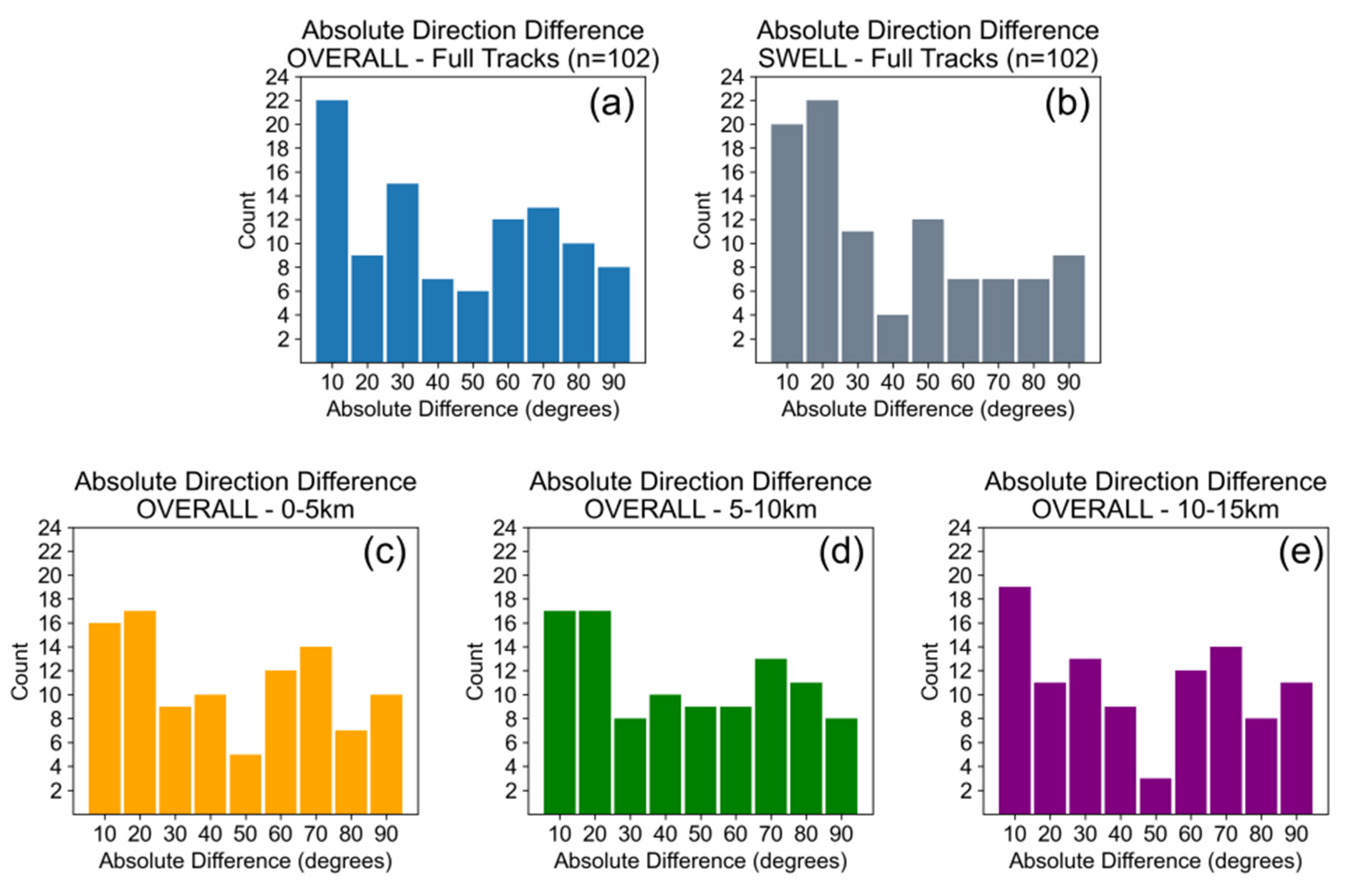
Figure 9.
Sentinel-1A synthetic aperture radar image (VV polarization) illustrating some of the complex wave dynamics around Oahu. Image taken 2020-Dec-19.
Figure 9.
Sentinel-1A synthetic aperture radar image (VV polarization) illustrating some of the complex wave dynamics around Oahu. Image taken 2020-Dec-19.
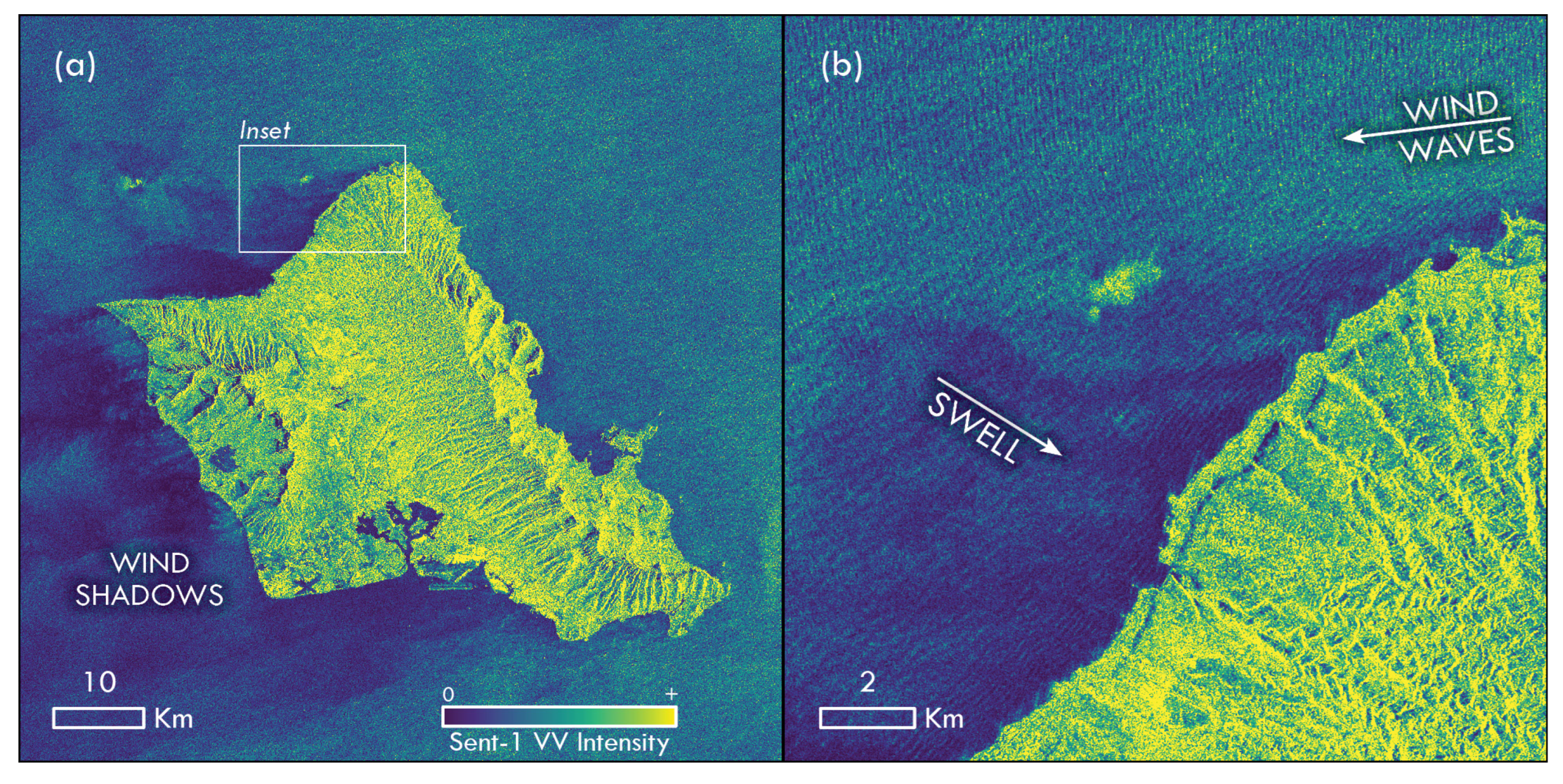
Table 1.
Apparent wavelength factor and theoretical left/right offset distances for a range of wave directions relative to ICESat-2's orbital inclination.
Table 1.
Apparent wavelength factor and theoretical left/right offset distances for a range of wave directions relative to ICESat-2's orbital inclination.
| Compass Angle | Apparent Wavelength Factor | Theoretical Offset Distance (Directionality) |
|---|---|---|
| 0 / 180° | 100.1% | 3.1428 |
| 15 / 195° | 104.6% | 27.5009 |
| 30 / 210° | 117.9% | 56.2059 |
| 45 / 225° | 146.6% | 96.4563 |
| 60 / 240° | 213.0% | 169.1642 |
| 75 / 255° | 444.5% | 389.5973 |
| 86-90 / 266-270° | 2865% - ∞ | 2577 - ∞ |
| 105 / 285° | 342.0% | -294.195 |
| 120 / 300° | 188.7% | -143.94 |
| 135 / 315° | 136.7% | -83.8733 |
| 150 / 330° | 113.3% | -47.8228 |
| 165 / 345° | 102.6% | -20.7636 |
| 180 / 0° | 100.1% | 3.1428 |
Disclaimer/Publisher’s Note: The statements, opinions and data contained in all publications are solely those of the individual author(s) and contributor(s) and not of MDPI and/or the editor(s). MDPI and/or the editor(s) disclaim responsibility for any injury to people or property resulting from any ideas, methods, instructions or products referred to in the content. |
© 2024 by the authors. Licensee MDPI, Basel, Switzerland. This article is an open access article distributed under the terms and conditions of the Creative Commons Attribution (CC BY) license (https://creativecommons.org/licenses/by/4.0/).
Copyright: This open access article is published under a Creative Commons CC BY 4.0 license, which permit the free download, distribution, and reuse, provided that the author and preprint are cited in any reuse.


