
Submitted:
10 March 2025
Posted:
11 March 2025
You are already at the latest version
Abstract
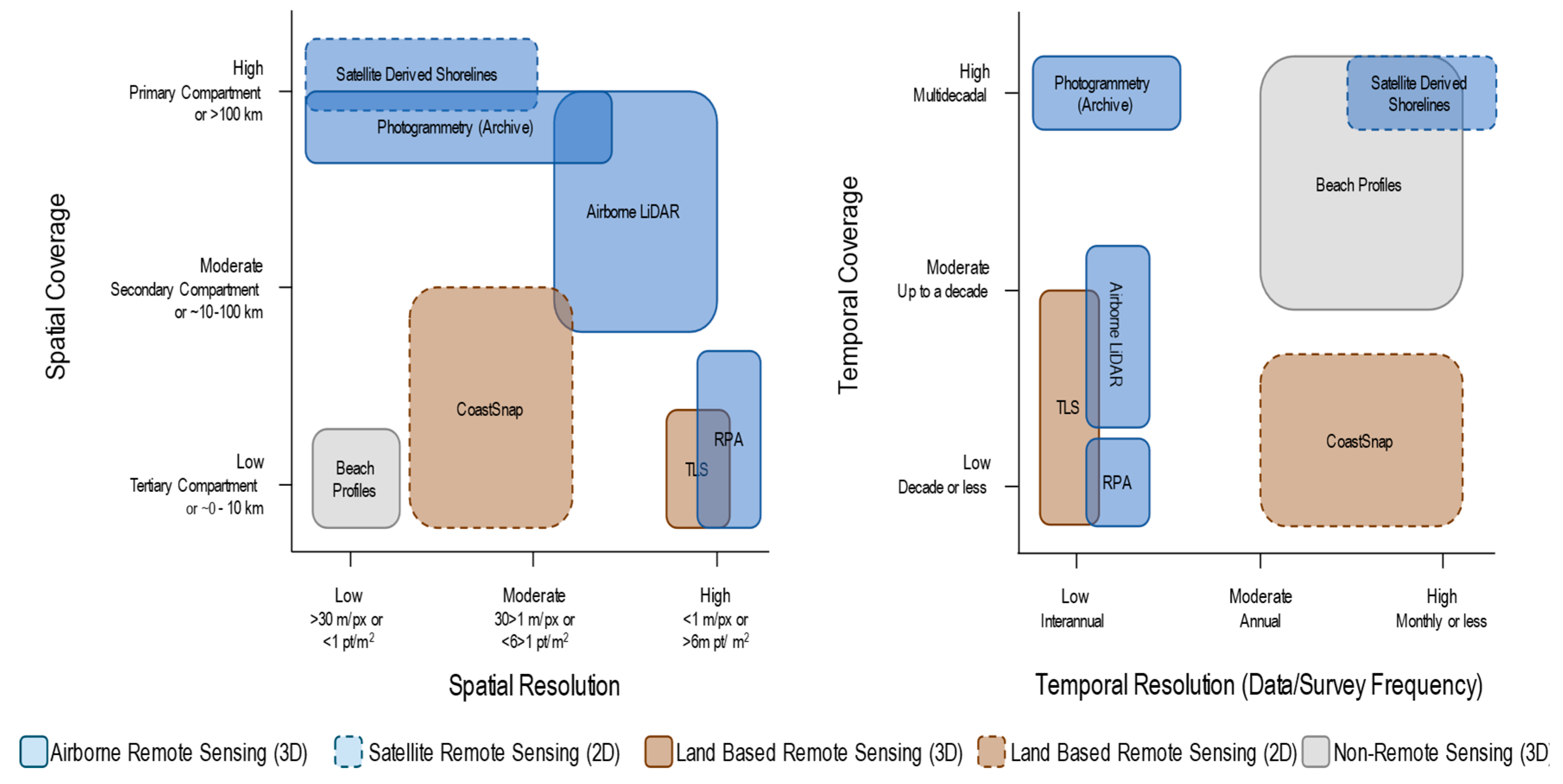
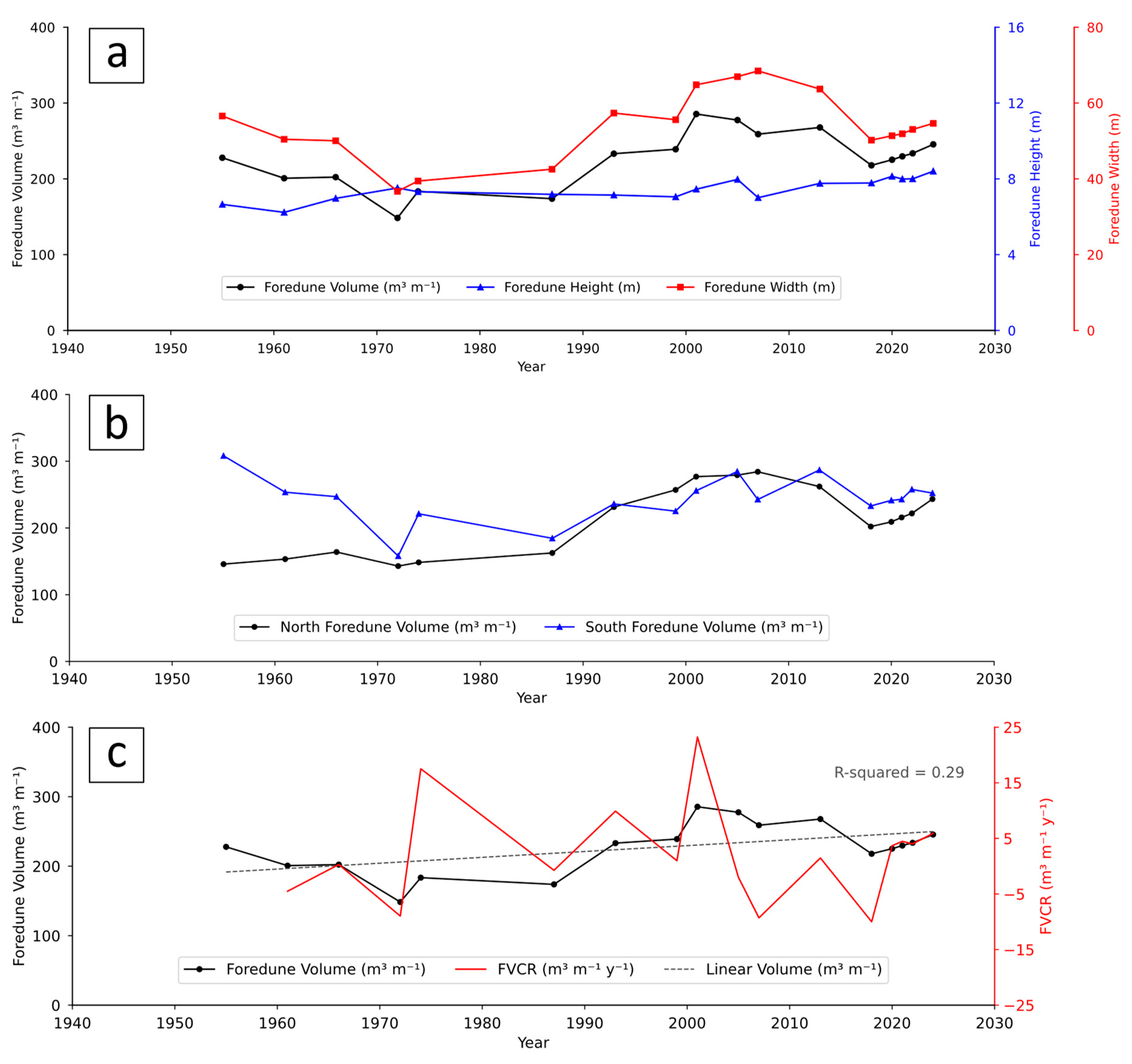
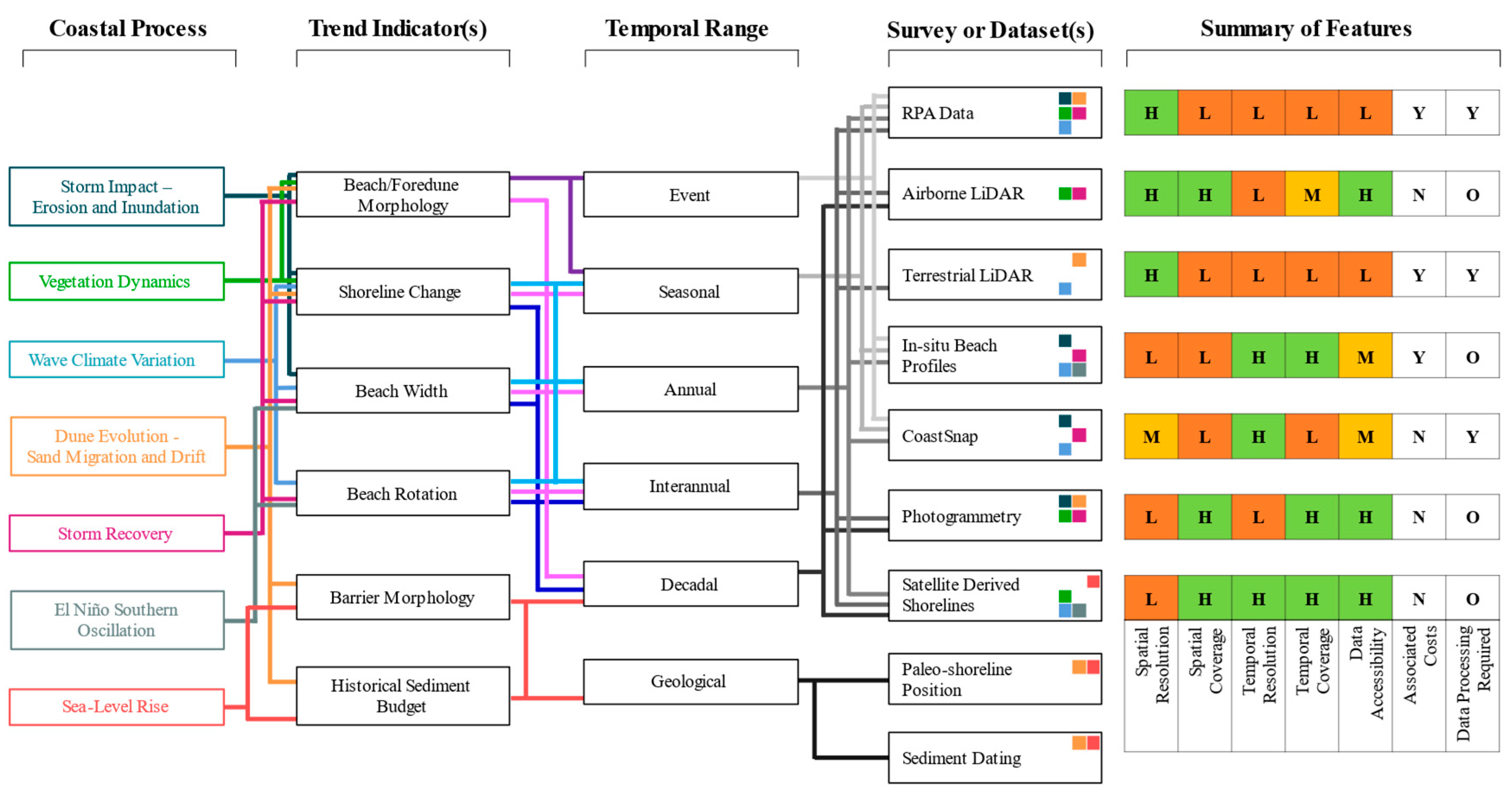
To support coastal practitioners and decision makers manage the complex coastal zone a structured framework was developed to navigate a range of technologies, datasets and data-derived products based on their suitability to monitor the spatial and temporal diversity of coastal processes and morphological indicators. Remote piloted aircraft (RPA) fitted with a LiDAR sensor was used in conjunction with airborne LiDAR and photogrammetry data to undertake foredune change analyses for selected sites in southeastern Australia to validate and demonstrate optimal technology for coastal monitoring. Results were compared with satellite derived coastal change products, including the Digital Earth Australia Coastlines and CoastSat. Foredune volumes from the mid-1900s to 2024 at the highly modified and urbanised Woonona-Bellambi and Warilla Beaches exhibited long-term stability interrupted by large storm events and anthropogenic interventions. Satellite derived data from 1988 onwards showed shoreline regions experiencing the highest rates of seaward extension and landward retreat. The high temporal resolution of this data supports monitoring changes, such as the influence of the El Niño Southern Oscillation on beach rotation. Photogrammetry data with multidecadal temporal coverage provides insights into historical changes. Airborne LiDAR offers three-dimensional data with high spatial resolution to develop accurate terrain models as LiDAR pulses can penetrate foredune vegetation. RPA LiDAR and aerial image data delivered the highest spatial resolution of the beach and foredune region and improves capacity to understand and describe sediment dynamics within a beach or compartment. Rapid deployment capability of RPAs allows for immediate evaluation of impacts from episodic events including storms and management interventions, thereby enhancing hazard mitigation efforts, and improving knowledge of coastal processes. The framework presented in this study emphasises the importance of integrating complimentary monitoring technologies and datasets to improve the temporal and spatial relevance of projections that inform coastal management.
Keywords:
Introduction
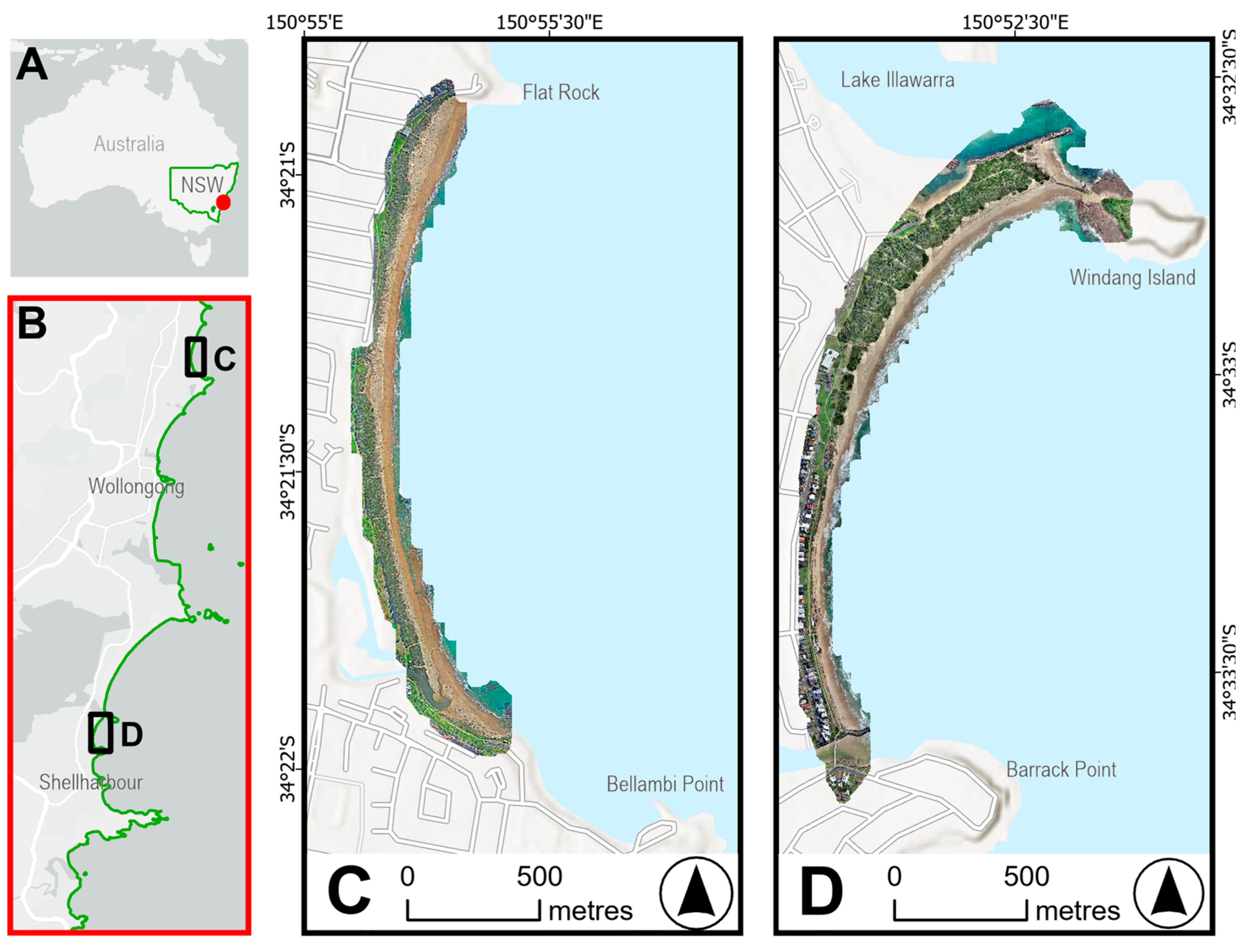
Regional Setting
Materials and Methods
Coastal Data Types
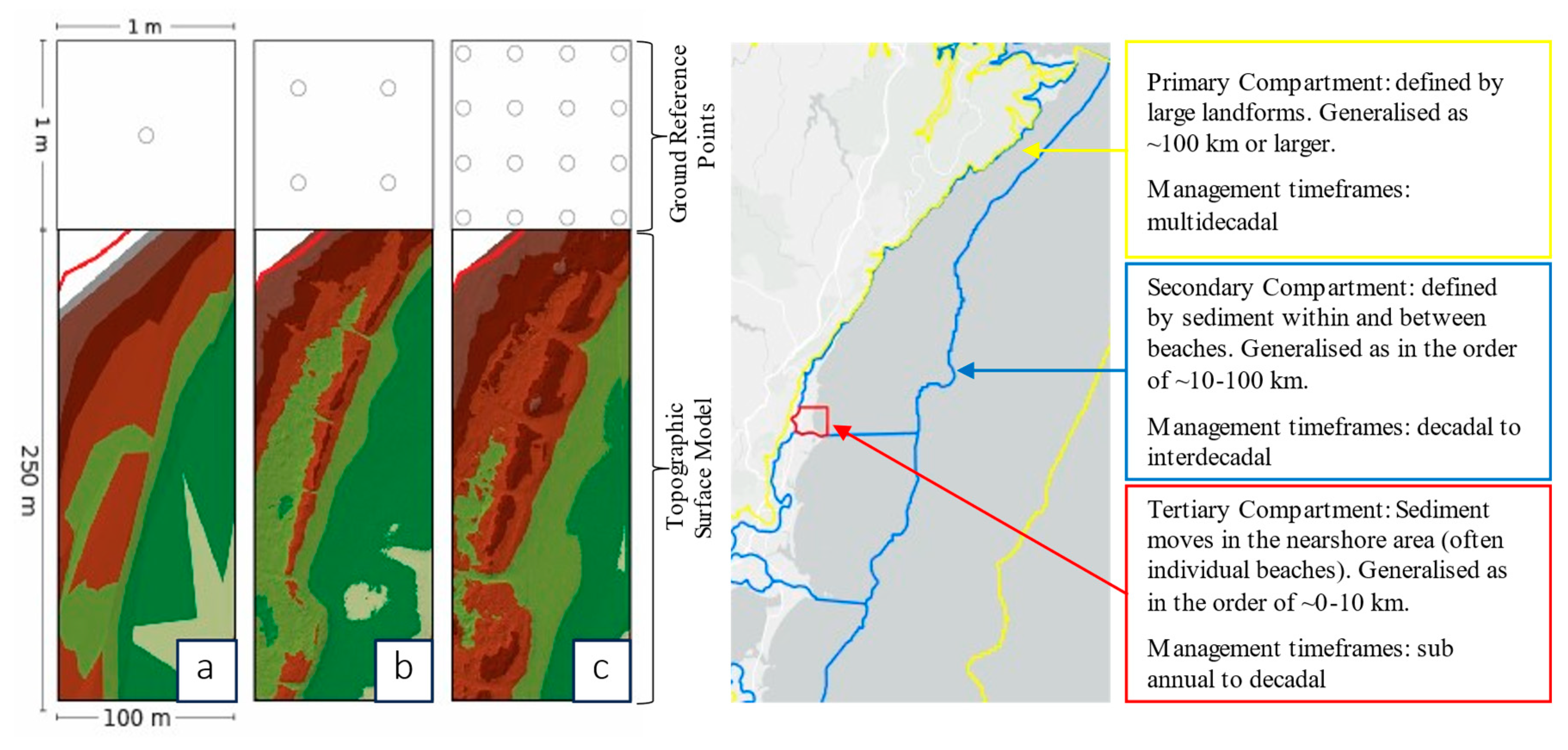
Spatial and Temporal Criteria
Topographic Data Capture and Analysis
Foredune Geomorphic Change Analysis
Results
Coastal Data – Resolution and Coverage
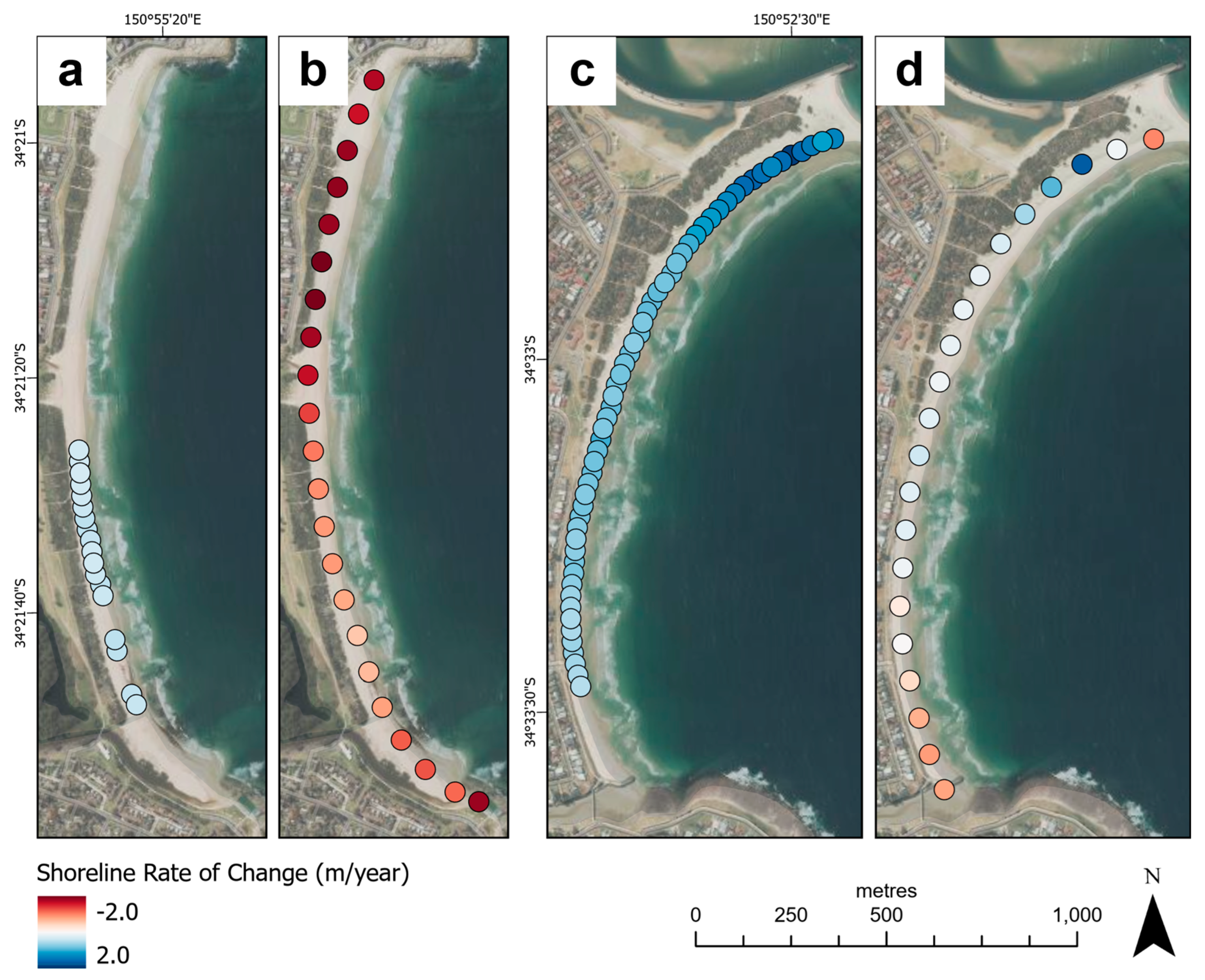
Coastal Data–Shorelines and Foredunes
Woonona-Bellambi Beach
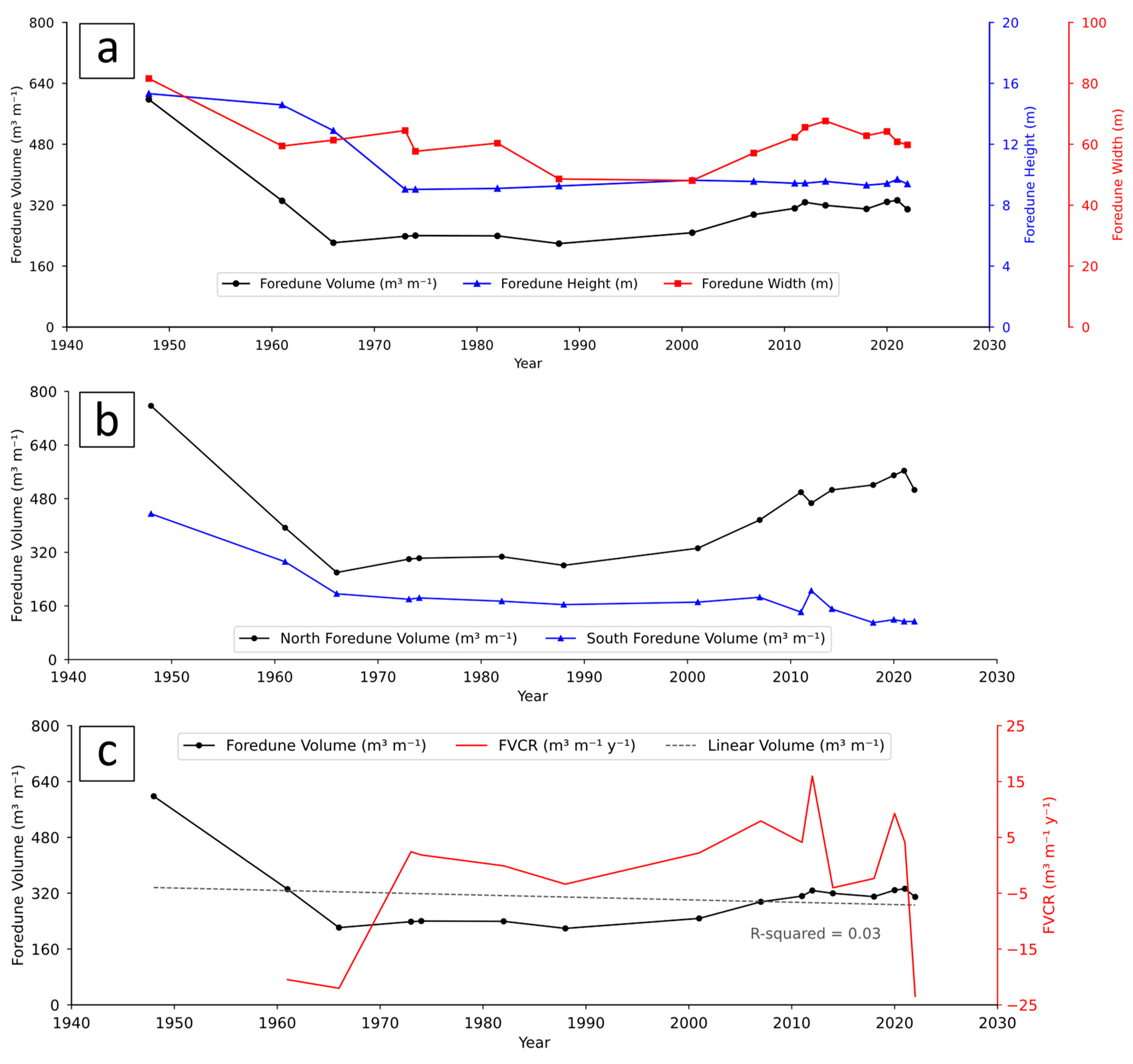
Warilla Beach
Discussion
Coastal Data–Shorelines and Foredunes
Coastal Data–Resolution and Coverage
Appendix
Appendix 1: Flight and sensor parameters for DJI M300 and L1 LiDAR sensor for 2024 surveys.
| RPA: DJI Matrice M300 with DJI L1 Zenmuse LiDAR sensor with EP800 camera | |
| Flight Date: Tuesday 28 May 2024 | |
| Flight and Sensor Details | |
| Average altitude (m) | 60 |
| Area flown (km2) | 0.3 |
| Independent GCPs | 17 |
| Side Overlap (LiDAR) (%) | 50 |
| Return Mode (LiDAR) | Triple |
| Sampling Rate (LiDAR) (KHz) | 160 |
| Point Cloud Density (pts/m2) | 327 |
| Ortho Ground Sample Distance (GSD) (cm/px) | 1.64 |
| Image Bands | Red (0.64-0.67µm) Green (0.53-0.59µm) Blue (0.45-0.51µm) |
| RTK Corrections | Yes – NSW CORSNet via NTRIP |
| Processing Parameters | |
| DJI Terra Software Version | 3.7.6 |
| Cloud point density | High (100%) |
| Optimize Point Cloud Accuracy | Yes |
| Smooth Point Cloud | Yes |
| Projected Coordinate System (EPSG) | 7844 |
| Returns | 3 |
| Output Files | PNTS file LAS file |
References
- Asbridge, E., Clark, R., Denham, P., Hughes, M. G., James, M., McLaughlin, D., Turner, C., Whitton, T., Wilde, T., & Rogers, K. (2024). Tidal Impoundment and Mangrove Dieback at Cabbage Tree Basin, NSW: Drivers of Change and Tailored Management for the Future. Estuaries and Coasts, 47(8), 2190-2208. [CrossRef]
- Banno, M., Nakamura, S., Kosako, T., Nakagawa, Y., Yanagishima, S.-i., & Kuriyama, Y. (2020). Long-Term Observations of Beach Variability at Hasaki, Japan. Journal of Marine Science and Engineering, 8(11). [CrossRef]
- Bauer, B. O., Ollerhead, J., Delgado-Fernandez, I., & Davidson-Arnott, R. G. D. (2025). Analyzing topographic change profiles in coastal foredune systems: Methodological recommendations. Geomorphology, 472, 109610. [CrossRef]
- Bertin, S., Floc’h, F., Le Dantec, N., Jaud, M., Cancouët, R., Franzetti, M., Cuq, V., Prunier, C., Ammann, J., Augereau, E., Lamarche, S., Belleney, D., Rouan, M., David, L., Deschamps, A., Delacourt, C., & Suanez, S. (2022). A long-term dataset of topography and nearshore bathymetry at the macrotidal pocket beach of Porsmilin, France. Scientific Data, 9(1), 79. [CrossRef]
- Bishop-Taylor, R., Nanson, R., Sagar, S., & Lymburner, L. (2021). Mapping Australia's dynamic coastline at mean sea level using three decades of Landsat imagery. Remote Sensing of Environment, 267. [CrossRef]
- Bishop-Taylor, R., Sagar, S., Lymburner, L., & Beaman, R. J. (2019). Between the tides: Modelling the elevation of Australia's exposed intertidal zone at continental scale. Estuarine, Coastal and Shelf Science, 223, 115-128. [CrossRef]
- Carvalho, R. C., Allan, B., Kennedy, D. M., Leach, C., O'Brien, S., & Ierodiaconou, D. (2021). Quantifying decadal volumetric changes along sandy beaches using improved historical aerial photographic models and contemporary data. Earth surface processes and landforms, 46(10), 1882-1897. [CrossRef]
- Carvalho, R. C., & Woodroffe, C. D. (2023). Coastal compartments: the role of sediment supply and morphodynamics in a beach management context. Journal of Coastal Conservation, 27(6). [CrossRef]
- Chataigner, T., Yates, M. L., Le Dantec, N., Harley, M. D., Splinter, K. D., & Goutal, N. (2022). Sensitivity of a one-line longshore shoreline change model to the mean wave direction. Coastal Engineering, 172, 104025. [CrossRef]
- Clarke, D. J., & Eliot, I. G. (1988). Low-frequency changes of sediment volume on the beachface at Warilla Beach, New South Wales, 1975–1985. Marine Geology, 79(3), 189-211. [CrossRef]
- Cohn, N., Brodie, K., Conery, I., & Spore, N. (2022). Alongshore Variable Accretional and Erosional Coastal Foredune Dynamics at Event to Interannual Timescales. Earth and Space Science, 9(12). [CrossRef]
- Cooper, J. A. G., Masselink, G., Coco, G., Short, A. D., Castelle, B., Rogers, K., Anthony, E., Green, A. N., Kelley, J. T., Pilkey, O. H., & Jackson, D. W. T. (2020). Sandy beaches can survive sea-level rise. Nature Climate Change, 10(11), 993-995. [CrossRef]
- Cooper, J. A. G., & Pilkey, O. H. (2004). Sea-level rise and shoreline retreat: time to abandon the Bruun Rule. Global and Planetary Change, 43(3), 157-171. [CrossRef]
- Davidson-Arnott, R., Ollerhead, J., George, E., Houser, C., Bauer, B., Hesp, P., Walker, I., Delagado-Fernandez, I., & Van Proosdij, D. (2024). Assessing the impact of hurricane Fiona on the coast of PEI National Park and implications for the effectiveness of beach-dune management policies. Journal of Coastal Conservation, 28(3). [CrossRef]
- Davidson-Arnott, R., Hesp, P., Ollerhead, J., Walker, I., Bauer, B., Delgado-Fernandez, I., & Smyth, T. (2018). Sediment budget controls on foredune height: Comparing simulation model results with field data. Earth Surface Processes and Landforms, 43(9), 1798-1810. [CrossRef]
- Doyle, T. B., Hesp, P. A., & Woodroffe, C. D. (2024). Foredune morphology: Regional patterns and surfzone–beach–dune interactions along the New South Wales coast, Australia. Earth Surface Processes and Landforms, 49(10), 3115-3138. [CrossRef]
- Doyle, T. B., Short, A., & Woodroffe, C. D. (2019a). Foredune evolution in eastern Australia: A management case study on Warilla Beach Coastal Sediments 2019.
- Doyle, T. B., Short, A. D., Ruggiero, P., & Woodroffe, C. D. (2019b). Interdecadal Foredune Changes along the Southeast Australian Coastline: 1942–2014. Journal of Marine Science and Engineering, 7(6), 177. https://www.mdpi.com/2077-1312/7/6/177.
- Doyle, T. B., & Woodroffe, C. D. (2018). The application of LiDAR to investigate foredune morphology and vegetation. Geomorphology, 303, 106-121. [CrossRef]
- Doyle, T. B., & Woodroffe, C. D. (2023). Modified foredune eco-morphology in southeast Australia. Ocean & Coastal Management, 240, 106640. [CrossRef]
- Eliot, I. G., & Clarke, D. J. (1982). Seasonal and biennial fluctuation in subaerial beach sediment volume on Warilla Beach, New South Wales. Marine Geology, 48(1), 89-103. [CrossRef]
- Evans, P., & Hanslow, D. J. (1996). Take a Long Line -Risk and Reality in Coastal Hazard Assessment 6th NSW Coastal Conference, Ulladulla, Australia.
- Fellowes, T. E., Vila-Concejo, A., Gallop, S. L., Schosberg, R., de Staercke, V., & Largier, J. L. (2021). Decadal shoreline erosion and recovery of beaches in modified and natural estuaries. Geomorphology, 390, 107884. [CrossRef]
- Gangaiya, P., Beardsmore, A., & Miskiewicz, T. (2017). Morphological changes following vegetation removal and foredune re-profiling at Woonona Beach, New South Wales, Australia. Ocean & Coastal Management, 146, 15-25. [CrossRef]
- Hague, B. S., Jakob, D., Kirezci, E., Jones, D. A., Cherny, I. L., & Stephens, S. A. (2024). Future frequencies of coastal floods in Australia: a seamless approach and dataset for visualising local impacts and informing adaptation. Journal of Southern Hemisphere Earth Systems Science, 74(3). [CrossRef]
- Hanslow, D. J. (2007). Beach Erosion Trend Measurement: A Comparison of Trend Indicators. Journal of Coastal Research, 588-593. http://www.jstor.org/stable/26481655.
- Hanslow, D. J., Morris, B. D., Foulsham, E., & Kinsela, M. A. (2018). A Regional Scale Approach to Assessing Current and Potential Future Exposure to Tidal Inundation in Different Types of Estuaries. Scientific Reports, 8(1). [CrossRef]
- Harley, M. D., & Kinsela, M. A. (2022). CoastSnap: A global citizen science program to monitor changing coastlines. Continental Shelf Research, 245, 104796. [CrossRef]
- Harley, M. D., Turner, I. L., Kinsela, M. A., Middleton, J. H., Mumford, P. J., Splinter, K. D., Phillips, M. S., Simmons, J. A., Hanslow, D. J., & Short, A. D. (2017). Extreme coastal erosion enhanced by anomalous extratropical storm wave direction. Scientific Reports, 7(1), 6033. [CrossRef]
- Harley, M. D., Turner, I. L., Short, A. D., & Ranasinghe, R. (2011). Assessment and integration of conventional, RTK-GPS and image-derived beach survey methods for daily to decadal coastal monitoring. Coastal Engineering, 58(2), 194-205. [CrossRef]
- Harrison, A. J., Miller, B. M., Carley, J. T., Turner, I. L., Clout, R., & Coates, B. (2017). NSW beach photogrammetry: A new online database and toolbox Australasian Coasts & Ports 2017: Working with Nature, Barton, ACT.
- Hesp, P. (2002). Foredunes and blowouts: initiation, geomorphology and dynamics. Geomorphology, 48(1), 245-268. [CrossRef]
- Hesp, P. A. (2013). A 34 year record of foredune evolution, Dark Point, NSW, Australia. Journal of Coastal Research, 65(sp2), 1295-1300, 1296. [CrossRef]
- Hesp, P. A. (2025). The role of climate in determining foredune types and modes. Coastal Engineering Journal, 67(1), 3-11. [CrossRef]
- Hesp, P. A., Hernández-Calvento, L., Gallego-Fernández, J. B., Miot da Silva, G., Hernández-Cordero, A. I., Ruz, M.-H., & Romero, L. G. (2021). Nebkha or not? -Climate control on foredune mode. Journal of Arid Environments, 187, 104444. [CrossRef]
- Ierodiaconou, D., Kennedy, D. M., Pucino, N., Allan, B. M., McCarroll, R. J., Ferns, L. W., Carvalho, R. C., Sorrell, K., Leach, C., & Young, M. (2022). Citizen science unoccupied aerial vehicles: A technique for advancing coastal data acquisition for management and research. Continental Shelf Research, 244, 104800. [CrossRef]
- Jarmalavičius, D., Pupienis, D., Žilinskas, G., Janušaitė, R., & Karaliūnas, V. (2020). Beach-Foredune Sediment Budget Response to Sea Level Fluctuation. Curonian Spit, Lithuania. Water, 12(2), 583. [CrossRef]
- Joyce, K. E., Fickas, K. C., & Kalamandeen, M. (2023). The unique value proposition for using drones to map coastal ecosystems. Cambridge Prisms: Coastal Futures, 1, 1-26. [CrossRef]
- Kinsela, M., Morris, B., Linklater, M., & Hanslow, D. (2017). Second-Pass Assessment of Potential Exposure to Shoreline Change in New South Wales, Australia, Using a Sediment Compartments Framework. Journal of Marine Science and Engineering, 5(4), 61. [CrossRef]
- Kinsela, M. A., Hanslow, D. J., Carvalho, R. C., Linklater, M., Ingleton, T. C., Morris, B. D., Allen, K. M., Sutherland, M. D., & Woodroffe, C. D. (2022). Mapping the Shoreface of Coastal Sediment Compartments to Improve Shoreline Change Forecasts in New South Wales, Australia. Estuaries and Coasts, 45(4), 1143-1169. [CrossRef]
- Kinsela, M. A., Morris, B. D., Ingleton, T. C., Doyle, T. B., Sutherland, M. D., Doszpot, N. E., Miller, J. J., Holtznagel, S. F., Harley, M. D., & Hanslow, D. J. (2024). Nearshore wave buoy data from southeastern Australia for coastal research and management. Scientific Data, 11(1), 190. [CrossRef]
- Kroon, A., Larson, M., Möller, I., Yokoki, H., Rozynski, G., Cox, J., & Larroude, P. (2008). Statistical analysis of coastal morphological data sets over seasonal to decadal time scales. Coastal Engineering, 55(7), 581-600. [CrossRef]
- Lacey, E. M., & Peck, J. A. (1998). Long-Term Beach Profile Variations along the South Shore of Rhode Island, U.S.A. Journal of coastal research, 14(4), 1255-1264.
- Lin, Y.-C., Cheng, Y.-T., Zhou, T., Ravi, R., Hasheminasab, S., Flatt, J., Troy, C., & Habib, A. (2019). Evaluation of UAV LiDAR for Mapping Coastal Environments. Remote Sensing, 11(24), 2893. [CrossRef]
- Liu, J., Meucci, A., Liu, Q., Babanin, A. V., Ierodiaconou, D., Xu, X., & Young, I. R. (2023). A high-resolution wave energy assessment of south-east Australia based on a 40-year hindcast. Renewable Energy, 215, 118943. [CrossRef]
- Lobeto, H., Semedo, A., Lemos, G., Dastgheib, A., Menendez, M., Ranasinghe, R., & Bidlot, J.-R. (2024). Global coastal wave storminess. Scientific Reports, 14(1), 3726. [CrossRef]
- Ludka, B. C., Guza, R. T., O’Reilly, W. C., Merrifield, M. A., Flick, R. E., Bak, A. S., Hesser, T., Bucciarelli, R., Olfe, C., Woodward, B., Boyd, W., Smith, K., Okihiro, M., Grenzeback, R., Parry, L., & Boyd, G. (2019). Sixteen years of bathymetry and waves at San Diego beaches. Scientific Data, 6(1). [CrossRef]
- McCarroll, R. J., Kennedy, D. M., Liu, J., Allan, B., & Ierodiaconou, D. (2024). Design and application of coastal erosion indicators using satellite and drone data for a regional monitoring program. Ocean & Coastal Management, 253, 107146. [CrossRef]
- McLean, R., Thom, B., Shen, J., & Oliver, T. (2023). 50 years of beach–foredune change on the southeastern coast of Australia: Bengello Beach, Moruya, NSW, 1972–2022. Geomorphology, 439, 108850. [CrossRef]
- Mentaschi, L., Vousdoukas, M. I., Pekel, J.-F., Voukouvalas, E., & Feyen, L. (2018). Global long-term observations of coastal erosion and accretion. Scientific Reports, 8(1). [CrossRef]
- Mentaschi, L., Vousdoukas, M. I., Voukouvalas, E., Dosio, A., & Feyen, L. (2017). Global changes of extreme coastal wave energy fluxes triggered by intensified teleconnection patterns. Geophysical Research Letters, 44(5), 2416-2426. [CrossRef]
- Moore, L. J. (2000). Shoreline Mapping Techniques. Journal of Coastal Research, 16(1), 111-124. http://www.jstor.org/stable/4300016.
- Moore, L. J., Ruggiero, P., & List, J. H. (2006). Comparing Mean High Water and High Water Line Shorelines: Should Proxy-Datum Offsets be Incorporated into Shoreline Change Analysis? Journal of Coastal Research, 2006(224), 894-905, 812. [CrossRef]
- Morris, B. D., Foulsham, E., Laine, R., Wiecek, D., & Hanslow, D. (2016). Evaluation of Runup Characteristics on the NSW Coast. Journal of Coastal Research, 75(sp1), 1187-1191. [CrossRef]
- NSW Office of Environment & Heritage. (2019). Report of Survey NSW Marine LiDAR Project. Sydney, Australia. Prepared by FUGRO for NSW Government.
- NSW Public Works Department. (1989). Coastline hazard program - beach improvement projects. Annual report 1988/89. Sydney, Australia. NSW Government.
- O'Reilly, W. C., Olfe, C. B., Thomas, J., Seymour, R. J., & Guza, R. T. (2016). The California coastal wave monitoring and prediction system. Coastal Engineering, 116, 118-132. [CrossRef]
- Oliver, T. S. N., Kinsela, M. A., Doyle, T. B., & McLean, R. F. (2024). Foredune erosion, overtopping and destruction in 2022 at Bengello Beach, southeastern Australia. Cambridge Prisms: Coastal Futures, 2, 1-20. [CrossRef]
- Owers, C. J., Rogers, K., & Woodroffe, C. D. (2018). Terrestrial laser scanning to quantify above-ground biomass of structurally complex coastal wetland vegetation. Estuarine, Coastal and Shelf Science, 204, 164-176. [CrossRef]
- Phillips, M. S., Harley, M. D., Turner, I. L., Splinter, K. D., & Cox, R. J. (2017). Shoreline recovery on wave-dominated sandy coastlines: the role of sandbar morphodynamics and nearshore wave parameters. Marine Geology, 385, 146-159. [CrossRef]
- Psuty, N. P. (1988). Sediment budget and dune/beach interaction. Journal of Coastal Research, 1-4. http://www.jstor.org/stable/40928719.
- Pucino, N., Kennedy, D. M., Carvalho, R. C., Allan, B., & Ierodiaconou, D. (2021). Citizen science for monitoring seasonal-scale beach erosion and behaviour with aerial drones. Scientific Reports, 11(1). [CrossRef]
- Ranasinghe, R., McLoughlin, R., Short, A., & Symonds, G. (2004). The Southern Oscillation Index, wave climate, and beach rotation. Marine Geology, 204, 273-287. [CrossRef]
- RIEGL (2015). RIEGL VZ-1000 Datasheet, RIEGL Corporation. Horn, Austria. https://www.rieglusa.com/wp-content/uploads/datasheet-vz-1000-2015-03-24-1.pdf.
- Reguero, B. G., Losada, I. J., & Méndez, F. J. (2019). A recent increase in global wave power as a consequence of oceanic warming. Nature Communications, 10(1), 205. [CrossRef]
- Roger, E., Tegart, P., Dowsett, R., Kinsela, M. A., Harley, M. D., & Ortac, G. (2020). Maximising the potential for citizen science in New South Wales. Australian Zoologist, 40(3), 449-461. [CrossRef]
- Ruggiero, P., Kaminsky, G. M., Gelfenbaum, G., & Cohn, N. (2016). Morphodynamics of prograding beaches: A synthesis of seasonal- to century-scale observations of the Columbia River littoral cell. Marine Geology, 376, 51-68. [CrossRef]
- Short, A. D. (2007). Beaches of the New South Wales coast : a guide to their nature, characteristics, surf and safety (2nd ed.). Sydney University Press.
- Short, A. D. (2022). Australian beach systems: Are they at risk to climate change? Ocean & Coastal Management, 224, 106180. [CrossRef]
- Short, A. D., Trembanis, A. C., & Turner, I. L. (2001, 2001). Beach Oscillation, Rotation and the Southern Oscillation, Narrabeen Beach, Australia.
- Sivanandam, P., Turner, D., & Lucieer, A. (2022). Drone Data Collection Protocol using DJI Matrice 300 RTK: Imagery and Lidar Version 3.0.
- Splinter, K. D., Harley, M. D., & Turner, I. L. (2018). Remote Sensing Is Changing Our View of the Coast: Insights from 40 Years of Monitoring at Narrabeen-Collaroy, Australia. Remote Sensing, 10(11), 1744. [CrossRef]
- Strypsteen, G., Houthuys, R., & Rauwoens, P. (2019). Dune Volume Changes at Decadal Timescales and Its Relation with Potential Aeolian Transport. Journal of Marine Science and Engineering, 7(10), 357. [CrossRef]
- Thom, B. G., Eliot, I., Eliot, M., Harvey, N., Rissik, D., Sharples, C., Short, A. D., & Woodroffe, C. D. (2018). National sediment compartment framework for Australian coastal management. Ocean & Coastal Management, 154, 103-120. [CrossRef]
- Turner, I., Harley, M., & Drummond, C. (2016a). UAVs for coastal surveying. Coastal Engineering, 114, 19-2. [CrossRef]
- Turner, I., Harley, M. D., Short, A. D., Simmons, J. A., Bracs, M. A., Phillips, M. S., & Splinter, K. D. (2016b). A multi-decade dataset of monthly beach profile surveys and inshore wave forcing at Narrabeen, Australia. Scientific Data, 3(1), 160024. [CrossRef]
- Vos, K., Harley, M. D., Splinter, K. D., Simmons, J. A., & Turner, I. L. (2019a). Sub-annual to multi-decadal shoreline variability from publicly available satellite imagery. Coastal Engineering, 150, 160-174. [CrossRef]
- Vos, K., Harley, M. D., Turner, I. L., & Splinter, K. D. (2023). Pacific shoreline erosion and accretion patterns controlled by El Niño/Southern Oscillation. Nature Geoscience, 16(2), 140-146. [CrossRef]
- Vos, K., Splinter, K. D., Harley, M. D., Simmons, J. A., & Turner, I. L. (2019b). CoastSat: A Google Earth Engine-enabled Python toolkit to extract shorelines from publicly available satellite imagery. Environmental Modelling & Software, 122, 104528. [CrossRef]
- Walker, I. J., Davidson-Arnott, R. G. D., Bauer, B. O., Hesp, P. A., Delgado-Fernandez, I., Ollerhead, J., & Smyth, T. A. G. (2017). Scale-dependent perspectives on the geomorphology and evolution of beach-dune systems. Earth-Science Reviews, 171, 220-253. [CrossRef]
- Wang, J., Wang, L., Feng, S., Peng, B., Huang, L., Fatholahi, S. N., Tang, L., & Li, J. (2023). An Overview of Shoreline Mapping by Using Airborne LiDAR. Remote Sensing, 15(1), 253. [CrossRef]
- Woodroffe, C., Cowell, P., Callaghan, D., Ranasinghe, R., Jongejan, R., Wainwright, D. J., Barry, S., Rogers, K., & Dougherty, A. (2012). Approaches to risk assessment on Australian coasts: a model framework for assessing risk and adaptation to climate change on Australian coasts: final report.
- Woodroffe, C. D., & Murray-Wallace, C. V. (2012). Sea-level rise and coastal change: the past as a guide to the future. Quaternary Science Reviews, 54, 4-11. [CrossRef]
- Wulder, M. A., Roy, D. P., Radeloff, V. C., Loveland, T. R., Anderson, M. C., Johnson, D. M., Healey, S., Zhu, Z., Scambos, T. A., Pahlevan, N., Hansen, M., Gorelick, N., Crawford, C. J., Masek, J. G., Hermosilla, T., White, J. C., Belward, A. S., Schaaf, C., Woodcock, C. E., . . . Cook, B. D. (2022). Fifty years of Landsat science and impacts. Remote Sensing of Environment, 280, 113195. [CrossRef]
- Zarnetske, P. L., Ruggiero, P., Seabloom, E. W., & Hacker, S. D. (2015). Coastal foredune evolution: the relative influence of vegetation and sand supply in the US Pacific Northwest. Journal of The Royal Society Interface, 12(106), 20150017. [CrossRef]
- Zhang, J., & Larson, M. (2021). Decadal-scale subaerial beach and dune evolution at Duck, North Carolina. Marine Geology, 440, 106576. [CrossRef]

| Data or Survey Type | Woonona-Bellambi Beach Records | Warilla Beach Records | Spatial Resolution | Spatial Coverage | Temporal Resolution | Temporal Coverage | Considerations |
|---|---|---|---|---|---|---|---|
| RPA LiDAR | 2024, 2023 | 2023 | High | Low | Low | Low |
|
| Terrestrial Laser Scan | 2023, 2016 (2), 2015 (2), 2014, 2013 | 2023, 2010 | High | Low | Low | Low |
|
| Airborne LiDAR | 2021, 2018, 2013 | 2021, 2018, 2011 | High | High | Low | Moderate |
|
| On-ground Beach Profiles | 2013 to present | 1975 to 1985 | Low | Low | High | High |
|
| CoastSnap | - | 2021 to present | Moderate | Low | High | Moderate - Low |
|
| Photogrammetry | 2016, 2007, 2001, 1999, 1993, 1987, 1976, 1974, 1972, 1961, 1955 | 2014, 2011, 2007, 2001, 1988, 1982, 1974, 1973, 1966, 1961, 1948 | Low | High | Low | High |
|
| Satellite Derived Shorelines | 1988 to present | 1988 to present | Low | High | High | High |
|
Disclaimer/Publisher’s Note: The statements, opinions and data contained in all publications are solely those of the individual author(s) and contributor(s) and not of MDPI and/or the editor(s). MDPI and/or the editor(s) disclaim responsibility for any injury to people or property resulting from any ideas, methods, instructions or products referred to in the content. |
© 2025 by the authors. Licensee MDPI, Basel, Switzerland. This article is an open access article distributed under the terms and conditions of the Creative Commons Attribution (CC BY) license (http://creativecommons.org/licenses/by/4.0/).


