
Submitted:
18 September 2024
Posted:
19 September 2024
You are already at the latest version
Abstract
The Surface Water and Ocean Topography (SWOT) mission was launched on December 16, 2022 to measure water levels over both open ocean and inland waters. To achieve these objectives, the SWOT Payload contains an innovative Ka-band radar interferometer, called KaRIn, completed with a conventional nadir altimeter called POSEIDON-3C that has been switched on a month after launch and a few days before KaRIn. POSEIDON-3C measurements provide a link between large scale phenomena and high resolution. POSEIDON-3C design is based on POSEIDON-3B, its predecessor on-board JASON-3. It is also a dual frequency radar altimeter operating in C and Ku bands, but with some improvements to enhance its performance. Even though it is a Low Resolution Mode altimeter, its performances over open ocean, inland waters and coastal zones are indeed excellent.This paper first describes the POSEIDON-3C design, and its modes with a focus on its new features and its Digital Elevation Model that drives its open-loop tracking mode. Then we assess the in-flight performances of the altimeter from an instrumental point of view. For that purpose, special and routine calibrations have been realized. They show the good performances and stability of the radar. In-flight assessments give thus confidence to ensure excellent altimeter measurement stability throughout the mission duration.
Keywords:
POSEIDON‐3C
; SWOT
; altimeter
; nadir
; altimetry
; LRM
; DEM
; tracking
; calibration
; validation
1. Introduction
CNES and NASA have jointly developed and operate the SWOT (Surface Water and Ocean Topography) mission to measure water levels in oceans, rivers, lakes and flooded areas, and their spatio-temporal variations. The mission is based on a major breakthrough in the field of spatial altimetry: Ka-band simultaneous interferometry. This innovative technical concept makes it possible to improve the planimetric resolution of ocean observations by an order of magnitude, and to measure the height of the vast majority of continental water surfaces. The Ka-band radar interferometer, KaRIn, in charge of this high-resolution monitoring, is completed by a conventional altimetry payload, which is currently carried by the JASON series of satellites.
This classical altimetry payload includes a nadir altimeter called POSEIDON-3C, developed by Thales Alenia Space. This is a dual-frequency altimeter (C and Ku bands) that strongly inherits from POSEIDON-3B (the altimeter on-board the JASON-3 mission) but with a few additional improvements. It ensures the SWOT “high wavelength” performance, typically beyond 300km. It is also used to calibrate KaRIn crossover points and measure ionospheric delay. POSEIDON-3C is thus a link between large scale historical measurements and new high-resolution altimetry provided by KaRIn.
The POSEIDON-3C altimeter was powered up on January 16, 2023, exactly one month after the SWOT satellite was launched into orbit by a Falcon 9. It has been extensively characterized in flight since then, especially during the first six months of the mission, when SWOT was in a fast 1-day repeat orbit for the Cal/Val phase. In-flight assessment also continued after the orbit change that took place in July 2023 to reach the final 21-day repeat orbit of the Science phase. Since switch-on, POSEIDON-3C has been continuously working, demonstrating its excellent behavior and in-flight performance.
This paper aims at presenting the POSEIDON-3C altimeter on board the SWOT mission with a focus on the assessment of its instrumental performance that was carried out during the commissioning phase. A description of the POSEIDON-3C altimeter is given in Section 2. It recalls its measurement principle, presents its architecture and details then successively its tracking and calibration modes. The POSEIDON-3C in-flight assessment is then performed in Section 3: Section 3.2 is dedicated to the instrumental assessment over ocean, inland waters and coastal zones, Section 3.3 is dedicated to the long term monitoring of the instrument parameters, and Section 3.4 details the exceptional calibration activities that have been carried out during the checkout phase. The last section concludes this article.
2. POSEIDON-3C Altimeter Description
2.1. Altimeter Principle & Performance
The main purpose of an altimeter is to provide an accurate estimate of the distance between the instrument and the observed surface. In the case of a radar altimeter, the distance, also called range, is deduced from the estimated round-trip time of a microwave signal, usually modulated. In the case of the POSEIDON-3C altimeter, the principle is the same as all POSEIDON-type instruments: it uses the full deramp technique, which has been widely used for radar altimeters to reduce emitted power and sampling frequency while maintaining the desired range resolution [1].
2.1.1. The Full Deramp Technique
This technique is based on the transmission of a linearly frequency-modulated signal, called chirp (see Figure 1). During the reception interval, the reflected echo is mixed with an analog replica of the chirp. The resulting signal is then made up of beats whose frequencies (f) are linearly related to the round-trip time (td) of the targets backscattered of the surface by the relation:
where B is the bandwidth of the chirp and T the pulse duration. Frequency synthesis of this signal (in digital form) then gives the echo, referenced by the round-trip time. The range is finally calculated by the formula:
where c is the speed of light and d the distance between the instrument and the surface.
f = B × td/T,
td = 2d/c,
The full deramp technique brings two strong limitations:
- The range window (or observation window) is limited by the number of FFT samples.
- The range gate (frequency step of the FFT) is defined by the pulse duration.
The POSEIDON-3C instrument provides, as POSEIDON-3B, a 128 points FFT and a 105.6µs pulse duration which leads to a range window of 60m and a range gate of approximatively 47cm (corresponding to the radar range resolution). Since the altimeter operates at several hundreds of kilometers and the echo shape can be spread over multiple range bins, it is necessary to estimate the round trip time to be sure that the returned echo is in the range window. This estimation is performed by the processing unit (PCU see Section 2.2) either by using the closed-loop tracking mode or using open loop mode (see Section 2.3).
2.1.2. Propagation Biases Resolution
As the instrument measures a signal traveling from space to the Earth’s surface, propagation delays must be corrected in order to obtain an accurate range estimate. In particular, the ionosphere delay, which is dispersive, is resolved on ground by processing echoes at two frequencies. For POSEIDON-3C, Ku band (13.575 GHz) and C band (5.3 GHz) signals are used with a 3Ku-1C-3Ku interleaved chronogram (Ku band echoes are used for range estimation). Other biases impacting the range estimations, such as wet and dry tropospheric delay, atmospheric attenuation and sea-state bias, are corrected on the ground, using radiometer measurements from the AMR (Advanced Microwave Radiometer) and models. [2].
2.1.3. Performance Requirement and Improvement with Respect to POSEIDON-3B
The main objectives of the SWOT nadir payload are to complement the KaRIn instrument and to pursue the mission continuity objective of past and current nadir altimetry satellites. POSEIDON-3C development and design has a strong heritage of POSEIDON-3B. Therefore, POSEIDON-3C is expected to perform at least as well as its predecessor.
After the instrument has transmitted its telemetry, the main geophysical parameters (e.g., range, significant wave height, backscattering coefficient) are obtained from the on-ground processing by inversion of the backscattered echo, using a specific algorithm, models and instrument internal calibration (see Section 2.4) [3]. This step consists in the so-called retracking.
One of the factors limiting the restitution of echo parameters is speckle noise, a coherent noise induced by the random combination of the radar returns from the scatterers on the surface. This speckle noise is reduced onboard by incoherently summing pulses before transmitting the telemetry. Nominally 105 pulses are used, resulting in a telemetry cycle time of approximately 55 ms. Note that the Pulse Repetition Frequency (PRF) has been adapted to the SWOT orbits. The PRF was indeed equal to 1976 Hz for the 1-day repeat orbit at a mean altitude of 857 km. It was changed to 1906 Hz for the 21-day repeat orbit at a mean altitude of about 890 km.
For inland waters or ice, the limiting factor is the dynamic of the receiving chain, which must match that of the backscatter coefficient. For POSEIDON-3C, the 62 dB dynamic range of the gain control loop ensures unsaturated echoes over approximately 99 % of the total water surface overflown by the altimeter (see Section 3.2.5).
An important improvement over POSEIDON-3B is the increase in echo coding dynamics. While on POSEIDON-3B echoes are coded on 8 bits, POSEIDON-3C echoes are coded on 16 bits. The internal gain control loop setpoint has then been modified to improve the thermal noise resolution from one Least Significant Bit, (POSEIDON-3B) to three Least Significant Bits, (POSEIDON-3C), thus improving the estimation of echo parameters (see Section 3.2.2.3). Example of POSEIDON-3C echoes measured over ocean are shown in Figure 2.
2.2. POSEIDON-3C Architecture
The POSEIDON-3C architecture is similar to POSEIDON-3B, except that the electronic boxes are not redounded. The instrument is composed of a Processing and Control Unit (PCU), a Radio Frequency Unit (RFU) and a dual frequency antenna as shown in Figure 3.
2.2.1. Processing and Control Unit (PCU)
The PCU handles altimeter sequencing, signal processing and interfaces with the satellite. Based on the ultra-stable 10 MHz oscillator supplied by the DORIS payload, the PCU generates all the sequencing signals used by the altimeter, in particular the range instruction used for the deramp. The transmitted chirp and replica are transmitted by the PCU to the RFU at low frequency and with limited bandwidth. On reception, after analog mixing of the echo with the chirp replica (inside the RFU), the PCU is used to digitize and to process the signal, and to format the telemetry. The flight software is operated by a Digital Signal Processor inside the PCU, and the DEM is stored in a 1Mo memory, as for the POSEIDON-3B altimeter [4] The PCU includes also a power converter that generates the secondary voltages to power the altimeter’s electronic boards.
2.2.2. RadioFrequency Unit (RFU)
The RFU handles all the altimeter’s analog processing. For transmission, it multiplies the chirp given by the PCU, increases the frequency by upconversion and amplifies it using a Solid-State Power Amplifier (SSPA). An internal duplexer is used to switch the antenna signal from transmission to reception, or to loop the Rx and Tx channels to measure the target point response (PTR) of the altimeter. During reception, analog mixing with the replica takes place inside the RFU. The gain of the receive chain is adapted by a command given by the PCU (Automatic Gain Control AGC) to avoid saturation of the PCU’s analog-to-digital converter. To simplify the architecture, a single reception chain is used for both C- and Ku-band signals, with a switch used to select the correct channel.
2.2.3. Antenna
The dual-frequency antenna is used to transmit and receive both Ku-band and C-band signals. It has a circular reflector of 1.2 m in diameter, offering a theoretical 3 dB beamwidth of 1.28°. Four arms are used to support the C/Ku horn. The arm supporting the Ku guide is perpendicular to the Ku polarization. The arm supporting the C-band coaxial is perpendicular to the C polarization.
2.3. POSEIDON-3C Tracking Modes
As described in §2.1, the full deramp technique implies that the altimeter synchronizes the chirp replica with the returned signal in order to place the echo inside the range window. The estimation of the round trip time of the transmitted signal is performed onboard by a tracking algorithm. Historically, since TOPEX/POSEIDON mission the tracking of echoes was based on an autonomous algorithm, based on a slip/gate discriminator, which estimates all necessary parameters. Since JASON-2 mission (POSEIDON-3), new operating modes have been used (see Table 1), significantly enhancing the data availability, especially for coastal areas, land to water transitions and inland water measurement [4].
Building on this heritage, five tracking modes are implemented in the POSEIDON-3C instrument, using various combinations of acquisition and tracking capabilities. Table 1 shows an overview of these operating modes, which are described in Section 2.3.1 to 2.3.3.
2.3.1. Autonomous Acquisition and Tracking Mode (M1)
This autonomous mode is also called “median tracker” or “closed-loop mode”. In this mode, the instrument defines alone the adequate range instruction. The algorithm is divided into three phases: search, positioning and tracking. In the search phase, the set point varies over a predefined altitude range (~38 km for the 21-day orbit) calculated from the shape of the Earth’s geoid and the satellite’s orbit. The instrument computes the amount of power inside the range window is then compared to a target threshold. When a return echo is detected, the instrument goes into positioning phase, where the echo is precisely positioned over the range window (size of the window is +/- 30 m) using a median discriminator [4]. At this stage the range tracking and the automatic gain control loops are initialized. In the tracking phase, all loops are locked, estimating at each cycle the future range position and the gain of the RFU receiver chain. The instrument provides science data telemetry only during the tracking phase.
In search phase, the reception chain gain is firstly set to the lowest level to avoid any saturation. If no echo is detected over the altitude range, another search cycle is initialized considering a higher gain value.
From the user’s point of view, only the tracking phase is important. The duration of the search and positioning phases correspond to data unavailability. In nominal operations, switching from search & positioning to tracking mode takes from a few tens of milliseconds to a few seconds, resulting in a very short lack of data.
2.3.2. The DIODE Acquisition & Autonomous Tracking Mode (M2)
This mode takes advantage of the orbital information provided by the DORIS (Doppler Orbitography by Radiopositioning Integrated on Satellite) instrument to reduce the search phase of the echo. Every ten seconds, the DIODE (DORIS Immediate Orbit on-board Determination) navigator sends the precise satellite orbit positioning and relative altitude to the Earth’s geoid to the altimeter. At each PRF cycle, the instrument extracts the range set point deducted from the last DIODE telemetry bulletin. This a priori surface elevation information is used to reduce the altitude dynamics of the search phase, resulting in a total acquisition cycle (search & positioning) of less than 0.5 seconds. In tracking phase, the algorithm is the same as in the autonomous acquisition and tracking mode M1.
2.3.3. The DIODE & DEM Mode (M3 to M4bis)
Since JASON-2 mission, a DEM is stored on the nadir altimeter onboard memory (see Section 2.5). Adapted to POSEIDON-3C, the DEM contains the Earth’s surface altitude and auxiliary data sampled over all SWOT orbits (at a constant 0.01° on-orbit-position sampling) and compressed into the 1Mo memory. For SWOT, two DEMs have been used, one for the 1-day orbit, another one for the 21-day orbit. By coupling orbit information from the DIODE navigator (see Section 2.3.2) with its onboard DEM data, the altimeter is able to estimate the return position of the surface echo with an accuracy better than a few range bins (~few meters), provided that the onboard DEM information is correctly set. No acquisition cycle is needed as the instrument works in open loop.
In this case the altimeter is always in tracking mode and ensures that return echoes from the surface are always recorded. This mode has dramatically improved the altimeter data availability for inland waters, coastal area or land to water transition surfaces, especially where the closed loop algorithm is not able to track the return echo [4,5].
2.3.4. Transitions between Modes
The user has the possibility to authorize transitions between DIODE & DEM and DIODE acquisition & autonomous tracking modes. In standard configuration mode (M3), no transition is authorized, the altimeter goes from stand-by state to DIODE & DEM tracking mode (and vice versa). When automatic transition is enabled, the instrument either returns to acquisition mode (M4), or goes directly to autonomous tracking (M4bis) (see Figure 4). The selection between M4 and M4bis modes is stored in the auxiliary data of the DEM for each orbit segment. The transition information is set directly in the onboard DEM using a specific byte.
The altimeter operates mainly in open loop (M3), but this ability to switch from one mode to another improves data availability, especially for some waterbodies whose water level can vary greatly from one orbital cycle to the next, 21 days apart (see Section 3.2.3 and 3.2.4).
2.4. POSEIDON-3C Calibration Modes
The high accuracy of extracted echoe parameters depends largely on the stability of the instrument. Even if ground measurements enable us to characterize the instrument’s performance in detail, it is necessary to continue with in-flight calibrations in order to make use of the instrument’s slight drift during the product generation stages. In addition, these calibrations are analyzed during the altimeter lifetime to verify its condition.
For POSEIDON-3C, two operating modes are used to monitor three main parameters. CAL1 mode is used to measure both the Point Target Response (PTR, also named impulse response) and the attenuation steps stability of the receive gain channel (AGC CAL1). CAL2 mode is used to characterized the frequency response of the receive channel.
2.4.1. Calibration of the Point Target Response (CAL1)
In the so-called CAL1 mode, the instrument’s PTR is measured by looping the transmit chain back to the receive chain through the duplexer’s calibration path (i.e., the antenna and associated waveguide are by passed). Several parameters are extracted from the PTR, including the internal travel time (group delay), the power of the main lobe (corresponding to the power of the receive/transmit channels) and its overall shape. A change in PTR can have an impact not only on the position of the echo in the range window, but also on its shape. This calibration is performed regularly in-flight (see Section 3.3.2).
2.4.2. Calibration of Reception Gain Steps (AGC CAL1)
The gain of the receiver chain has been characterized on the ground for all the gain steps used by the internal gain control loop. However, gain changes slightly over the life of the satellite as a function of temperature, space radiations and component ageing. This variation could have an impact on the estimation of the backscattering coefficient σ0, and is therefore periodically monitored in flight (see Section 3.3.4). The calibration of these reception gain steps is performed through a set of PTR measurements (CAL1) with different gain controls. A complete measurement of the actual reception gains values takes about 30 minutes. So it is carried out when the satellite is over land, to limit data loss over ocean for users.
2.4.3. Calibration of Reception Filter (CAL2)
The frequency response of the receiving chain after mixing is not perfectly flat due to the presence of analog low pass filter in the reception chain (see Section 2.1). This results in a slight distortion of the received echoes, but this distortion is compensated on-ground with the actual reception filter. The amplitude of the reception filter is indeed measured periodically in-flight through the CAL2 mode (see Section 3.3.3). This calibration is realized by integrating the thermal noise of the receiver chain over a sufficiently long period of time for a specific AGC value.
2.5. POSEIDON-3C Digital Elevation Model
The Open-Loop (OL) tracking mode makes use of a DEM, sampled under the satellite’s orbit and uploaded on board, also called “OLTC tables” (Open-Loop Tracking Command). These tables are read on board during navigation and allow the POSEIDON-3C altimeter to quickly adjust its reception window in order to enhance acquisitions over the ocean, coastal regions, and more importantly over a number of pre-selected continental water bodies worldwide. Altimetry missions currently operating with OLTC (SENTINEL-3 A & B, JASON-3, SENTINEL-6-MF) show highly improved amount of data acquisition over the selected water bodies [5].
The OLTC has been implemented on SWOT during both its Cal/Val and Science phases. Both onboard tables have been generated by merging and sampling several sources of elevation data, including generic sources such as the 2001 Mean Sea Surface [6] and the ACE2 continental DEM [7], and databases of hydrology targets built specifically for the SWOT OLTC. These “hydrological targets” are defined by combining the theoretical ground track of the satellite with several state-of-the-art datasets such as HydroLakes, GRanD (Global Reservoir and Dam Database), or SWORD (the SWOT River Database), potentially completed by local targets provided by the scientific community. In total, 5 813 water bodies are listed in the 1-day sampling Cal/Val hydrology targets database, and 58 681 for the 21-day orbit (see Figure 5 and Figure 6).
The multiple elevation sources have then been merged and sampled under SWOT’s ground track (for both orbits) with a constant on-orbit position step of 0.01°, i.e., approximately every 1 kilometer on ground. Finally, given the limited memory capacity (1 Mo) on board SWOT, compression strategies are applied to optimize the OLTC tables, similarly to JASON-2 and JASON-3 [4].
It is important to note that the vertical resolution of the onboard command in constrained by the coding optimization scheme, i.e., not less than 2 meters between two consecutive values. However, this vertical resolution is of secondary importance because it is solely used to set the reception window for the return signal. The inland water level resolution accuracy (as good as a few centimeters) is finally ensured by the retracking algorithm performed on ground.
3. POSEIDON-3C In-Flight Assessment
3.1. Description of the In-Flight Assessment
The POSEIDON-3C radar altimeter has been turned on at 9:32 (UTC) on January 16, 2023. This date stated the beginning of the in-flight instrument’s assessment activities that will be described hereafter. These activities were part of the whole SWOT Commissioning Phase. Their aim was to validate the functionality and the performances of the instrument in flight.
The functional aspects were essentially analyzed by testing all instrument modes. The functional characterization of the tracking modes has been assessed showing improvement over inland water and coastal zones with respect to POSEIDON-3B on JASON-3. This is explained by the evolutions described previously in Section 2.1.3. The main results are presented in the following paragraphs.
Regarding instrumental performance, we can distinguish routine calibration activities, which enable us to analyze instrument performance over the long term, from exceptional calibration activities, which aim to verify specific in-flight performance. The results of these calibrations are detailed in the following Section 3.3 and 3.4.
The final performances in terms of altimetry products that have been assessed during the Calibration/Validation phase are fully described in [3].
3.2. Functional Assessment of POSEIDON-3C Tracking Modes
This section focuses on illustrating the altimeter functional characteristics that have been assessed since the launch. First it gives a status on how and when the different tracking modes have been modified. Then it presents how the Automatic Gain Control is used over ocean and how the OLTC mode allows to improve acquisition over hydrological targets. A focus on acquisitions statistics over coastal zones is finally given.
3.2.1. Altimeter Modes Assessment
The nadir altimeter behavior has been analyzed and verified using different instrument modes. This assessment has been mainly performed on the 1-day orbit at the beginning of the checkout phase. It was required to stay at least for 2 weeks in each tracking mode in order to record a sufficient amount of data for the statistical analysis.
Table 2 indicates scheduling of the tracking modes modifications.
The autonomous mode M1 (see Section 2.3.1) was implemented and tested as soon as the instrument was switched on. As it is highly reliable and does not depend on any external data, neither position nor DEM, it enabled a direct transition into tracking just after the nadir altimeter was switched on, while the satellite was still overflying the ground station.
The other tracking modes that take advantage of the DORIS data were then successfully implemented from the simplest to the most complex mode, as described in Section 2.3.2 and 2.3.3.
In summer 2023, the SWOT mission entered in the final science phase of global mapping. This has been achieved by changing the spacecraft orbit from the 1-day orbit to the 21-day orbit. Several propulsive maneuvers were thus conducted between July 11 and July 21, 2023, to reposition the satellite about 38 km higher.
During this orbit change period, we set the altimeter in stand-by mode. We then switched it into the autonomous tracking mode M1, once on the 21-day orbit in order to deliver altimeter data as soon as possible. The new DEM (see Section 2.5) was uploaded on September 12, 2023. After 3 weeks of verification and validation the altimeter switched to M4bis mode October 9, 2023.
3.2.2. Functional Characterization over Ocean
This section aims to assess the altimeter’s functional aspects over open ocean. To avoid land and ice contamination, latitude has therefore been limited to +/-55° and distance to the closest shoreline (GSHHG model: Global Self-consistent, Hierarchical, High-resolution Geography Database [8]) is always higher than 50km. Histograms and gridded maps have been computed over one full repetitive cycle of the science 21-day orbit, between 02/11/2023 and 23/11/2023. Comparisons to JASON-3 have been performed over two repetitive cycles to cover the same period (cycles 357-358, from 05/11/2023 to 25/11/2023).
3.2.2.1. Tracking
Over open ocean, the topography varies slowly compared to other surfaces such as sea-ice or inland waters, so the signal is easier to track with a robust algorithm. The Autonomous acquisition and tracking mode (M1) was historically designed for open ocean [4] and it performs expectedly well for POSEIDON-3C with less than 0.04 % of data lost over ocean for one repetitive SWOT cycle (see Table 3). The DIODE+DEM mode, also called “open-loop mode”, shows even better performances with less than 0.001 % of data loss. M2, M3 and M4 are not discussed here as they also show equivalent performances.
Note that with the closed-loop mode M1, we detected the instrument occasionally kept tracking on noise after some inland-to-ocean transitions, leading to a reduced data lost. These few observed artefacts totally disappeared with the M2/M3/M4bis modes and have not been encountered since.
Overall, tracking performance of POSEIDON-3C over open ocean is excellent and is consistent between tracking modes.
3.2.2.2. Automatic Gain Control
Figure 7 shows that over open ocean for the Ku-band, the AGC command typically varies between 25 dB and 40 dB depending on the roughness of the surface. This is expected because the roughness of the surface is directly linked to the amount of energy returned to the altimeter. The AGC therefore adapts to the surface to ensure that the amplitude stays within the expected range. The median AGC value over ocean is 30 dB and is considered as the typical “ocean” value that is used to program the routine CAL2. For the C-band, the AGC typically varies between 18 dB and 30 dB depending on the roughness of the surface and the median value over ocean is 21 dB.
3.2.2.2. SNR
The Signal to Noise Ratio (SNR) is an important metric to characterize the performance and quality of the instrument’s signal. It is computed here with the following equation:
where amplitude and thermal noise are extracted for the level-2 variables amplitude_ocean and noise_floor_ocean respectively. The amplitude is estimated by the retracking algorithm, and the thermal noise is computed by averaging the amplitude between range gates [12;16] of the waveform.
POSEIDON-3C exhibits an excellent Ku-band SNR on open ocean, averaging around 22.8 dB and varying between 20 dB and 28 dB. It is slightly better compared to the averaged 21.7 dB of its predecessor POSEIDON-3B (Figure 8). Another noticeable difference between the two instruments is the SNR histogram shape, which is more Gaussian for Poseidon3C and more inflated over extreme values for POSEIDON-3B. This is due to the 8-bits coding of the Jason-3 waveforms that have a dynamic of [0-255] power units (p.u.), inducing a quantification on the thermal noise. Indeed, since the SNR is high, the thermal noise usually varies between 0 and 2 p.u., which significantly limits the ability to observe the physical variations of the thermal noise.
Since POSEIDON-3C echoes are coded in 16 bits, a wider range of values is now possible, allowing for a better retrieval of the thermal noise for an equivalent SNR. Figure 9 shows an example of a typical oceanic “Brownian” echo [9] for SWOT and JASON-3 for a Significant Wave Height (SWH) of about 2.5 meters. Both echoes seem similar at first glance, but a zoom on the thermal noise (first gates of the waveforms) clearly demonstrates the benefits of the 16-bits coding to retrieve the physical variations of the thermal noise on POSEIDON-3C. Also one may notice echoes have a slight different behavior over the trailing edge part. This is mainly due to differences in the orbit altitude between JASON-3 and SWOT [3].
For the C-band, the SNR averages on open ocean around 16.7dB (not showed here).
Note that this section aimed at describing the functional characterization of the instrument over open ocean, using level-0 and level-1 data. A complete analysis of the performances over ocean at level-2 is detailed in [3].
3.2.3. Functional Characterization over Inland Waters
The POSEIDON-3C altimeter has two Open-Loop tracking modes (M4 and M4bis) using the on-board Digital Elevation Model. The two modes have a different way of managing the transitions between Open-Loop (OL) and Closed-Loop (CL) tracking modes, which are driven by a mode mask implemented in the OLTC tables, as illustrated in Figure 10. Indeed, it is sometimes better to be in CL when the target elevation is not well known or when there is no expected in-hydrological target.
In M4 mode, the tracker constantly adjusts the reception window before acquiring new data, when switching from OL to CL. This mode, which is nominal on JASON-3, is really robust in terms of probability of acquisition. This results however in a loss of data during about 0.5-0.8 seconds at each OL to CL transition, corresponding to a length of about 3.4 to 5.1 kilometers on the ground.
The M4bis mode is hence designed to capture echoes immediately after the transition, using the last OL command to position the tracker instead of spending some precious milliseconds to readjust it. The M4bis mode more is then more efficient than the classical M4 mode in terms of acquisition speed from OL to CL (see Figure 11). Consequently, the M4bis mode significantly reduces the amount of data losses, and it has been selected as the nominal acquisition mode for SWOT.
To characterize the quality of the acquisitions over the hydrological targets used to define the OLTC, an indicator flag, which is set to “True” if the three following criteria are met: sufficient maximal power of the waveform, adequate centering of the waveform peak, and satisfactory signal-to-noise ratio. The flag is called the “Presence flag” and accounts for a well-defined and exploitable waveform when it is “True”; its calculation methodology is detailed in [5]. The Presence flag is computed over every SWOT cycle, with excellent results in OL mode: since it was activated on the operational 21-day orbit, the proportion of well acquired targets (i.e., of “True” Presence flags) oscillates between 92% and 96%, on par with other altimetry missions operating with OLTC.
3.2.4. Functional Characterization over Coastal Zones
Over coastal zones, tracking performance is also excellent. Between 0 and 50km to the closest shoreline, about 1.5 % of data are lost in close-loop mode (M1), which is satisfactory considering that this mode is, by definition, not perfectly suited to handle drastic transitions [4]. In nominal open-loop mode (M4bis), coastal performance is similar to ocean performance with only 0.007 % data loss, confirming the expected effectiveness of this mode over ocean/land transitions (Table 4). An example of ocean-to-land transition is displayed in Figure 12, where the closed-loop and open-loop modes show similar behavior while approaching the coast, with coastal perturbation happening at the same moment. In open-loop mode, a parabola is visible, which is a typical and expected pattern at the shoreline due to the “hooking” effect: since the ocean is significantly brighter compared to the land, the altimeter is “hooked” to the brightest points in the footprint that are not at nadir, creating this parabola [10].
For the land-to-ocean case, Figure 13 shows a typical example where the closed-loop mode loses the signal after the coastline, as opposed to the open-loop mode that manages to track the ocean closer to the coast, without any data loss.
3.2.5. Saturation
As explained in Section 2.1.3, POSEIDON-3C echoes are coded in 16 bits, they can thus vary from 0 to 65,535 power units. The internal gain control loop has been tuned to be optimal over open ocean, therefore in the case of extremely peaky echoes that are usually encountered over sea-ice or inland waters, the coding dynamics might not be enough and the echo “saturates”, creating a peak or a plateau with a maximum value of 65,535 (Figure 14.a). These echoes must be either edited or adequately processed with dedicated retracking algorithms as they contain incorrect values around the maximum. Figure 14.b exhibits the locations of all saturated echoes encountered during one full cycle and as expected, saturated echoes are almost exclusively encountered over land or sea-ice.
Table 5 details the proportion of saturated waveforms for different surfaces that have been roughly defined using thresholds on latitude “lat” and distance to the closest shoreline “dist”. Is also contains the corresponding statistics for JASON-3, computed over the same period for comparison purposes.
As expected, no saturation is observed over open ocean: the few saturated echoes identified have been inspected and turned out to be located over atolls (very specular targets) or small islands not correctly identified by our editing. Saturated echoes are regularly encountered over sea-ice, land and coastal areas with a proportion ranging from 1 % to 3 % depending on the surface. Similar metrics are obtained with JASON-3, although one can note some differences especially for land where the proportion reaches almost 4 % for JASON-3 versus 1.5 % for SWOT: this is most likely due to the 16 bits coding that allows a better dynamic for SWOT, compared to the 8-bits coding implemented on JASON-3.
3.3. Long Term Monitoring
The routine calibrations are performed three times a day as it was for JASON-3. The baseline is to execute these sequences over pre-defined desert zones (Figure 15).
3.3.1. HK Temperatures
From the platform thermistors of the RFU and the DPU, located on the altimeter’s payload panel, the evolution of the in-orbit temperatures can be monitored, using the house-keeping telemetries collected by the SWOT platform. Figure 16 and Figure 17 show the evolution of the temperatures since the beginning of the SWOT mission for both bands (averaged over a one day sliding window) for the RFU and PCU, along with the solar incidence angle. Over the first year of operations, temperatures show a relatively stable long-term signal within the expected range, with cyclic variations having a characteristic pattern of approximately 60 days. This cyclic pattern is linked to the beta prime angle [11], inducing variations up to 10°C. A similar impact of the sun beta angle was observed on POSEIDON-4 and documented in [12]. This impact is however less important for the other POSEIDON-3 predecessors, embarked on JASON-2 and JASON-3, for which the platform thermal conditions are different due to different orbits and satellite accommodations. The sudden temperature drop observed in July 2023 is due to the altimeter restart after the orbital maneuvers performed to shift from the 1-day orbit to the science 21-day orbit. The data gap observed between 21st and 28th September 2023 is due to a platform anomaly.
3.3.2. CAL1 Monitoring
CAL1 sequences are performed daily and aim at monitoring the Point Target Response (PTR). They are performed 3 times per day in routine operations to correct data products for any potential altimeter drift and monitor the instrument’s health. Long term stability is ensured thanks to these regular operations.
As expected, the consistency between the in-flight PTR and the realigned ideal “squared sinc” is excellent for both the Ku-band and the C-band (Figure 18).
Several PTR parameters are monitored on a cyclic basis to control the instrument’s health. The Long-Term Monitoring (LTM) of the PTR is performed by averaging these parameters on a 10-days sliding window. The monitored parameters, directly extracted from the ground segment calibration products, are:
- The Internal Path Delay (IPD) that corresponds to the shift between the middle of the receiving window and the middle of the PTR. It is computed here using the half-power method,
- The Width of the Main Lobe (WML) of the PTR,
- The total power of the PTR,
- The peak-power and peak-position of the 5 first sidelobes,
- Dissymmetry between the right-hand and left-hand sides.
The long-term monitoring of the IPD, total power and WML are displayed in Figure 19 and Figure 20, for the Ku and C bands respectively. The HK temperature of the SSPA has been superimposed to each plot.
For the Ku-band, the IPD is approximately 100 cm. It has drifted by -1.7 mm over the first year of life, which is less than the corresponding JASON-3’s delay over its first year (-3 mm). The total power decreased by 0.34 dB which is slightly stronger than for JASON-3 (-0.20 dB) but still well within the expected range. The WML is overall stable with a dynamic of +/-0.3 mm that is totally driven by the on-board temperature variations.
For the C-band, the IPD is around 127 cm with a drift of -5 mm over the first year, which is a bit lower than the corresponding -6.5 mm obtained on JASON-3 over the same period. The total power decreased by 0.48 dB, which is stronger than for JASON-3 (-0.12 dB) but still stays within the expected range of variations to ensure mission longevity. The WML is less stable than Ku-band with a drift of ~1.3mm over the first year. Also, the IPD and total power in C-band show “ripple variations” and not linear decays, that is again due to the sensitivity to the on-board temperature variations. Note that the Ku-band seems less affected by this effect. Finally, the thermal drop from September 2023 induced a small but visible jump for the PTR parameters in both bands.
In terms of PTR shape, Figure 21 and Figure 22 show the evolution of the left-hand side and right-hand side of the Peak-Power for the 5 first sidelobes, for the Ku-band. Both sides are stable in time, whether in position or in amplitude. Conclusions are similar for the secondary band (not showed here). The evolution of the PTR shape can also be assessed by looking at the left/right symmetry, i.e., by comparing the positions and powers of each right/left sidelobes peaks.
Figure 23 shows that the dissymmetry is stable with a variation range for each sidelobe that does not exceed +/-0.2 dB for the peak-power and +/-3 mm for the peak-position. Again, variations seem mostly driven by the on-board temperature variations. An altimeter restart on 22/06/2023 induced a visible plateau for all PTR shape parameters, especially for the 4th sidelobe in Ku-band with a right/left dissymmetry that jumped +1.2 dB (Figure 23). Later, another restart happened on 12/09/2023, and variations returned to their pre-plateau values. Note that restarts also induced variations of the same order of magnitude for JASON-3.
The evolution of the PTR through time is taken into account differently depending on the ground segment algorithms. Numerical retrackers, such as the Adaptive retracker [13,14] directly take the real in-flight PTR as an input of the algorithm, therefore any variation is naturally introduced, and it is the optimal option to correct the scientific outputs from the instrumental ageing. Historical ocean retrackers such as the MLE4 [15] include the IPD and the total power variations in the range and sigma0 instrumental corrections, but any significant shape variations (dissymmetry or WML variations) are not directly taken into account, which is why it is essential to monitor these parameters throughout the whole mission lifespan.
3.3.3. CAL2 Monitoring
As described in Section 2.4.3, the CAL2 sequence aims at monitoring the altimeter’s thermal noise response which is driven by the transfer function of the low-pass filter (LPF). This filter must be compensated for during ground processing, therefore its variations must be carefully monitored as it can impact the scientific variables in case of unexpected variations. Its global shape is similar to the other filters from the POSEIDON-3 family, and the 12 first and last gates are discarded during ground processing, therefore all metrics computed in this section consider only gates [12:116]. The in-flight LPF behaves similarly to the ground LPF but exhibits a more significant slope (Figure 24), which is not an issue since the real in-flight calibrations are directly used on-ground.
The Low-Pass Filter has been routinely monitored since the altimeter’s switch-on and shows an overall excellent stability since launch (Figure 25). For the Ku-band, over the useful window [12;116], the LPF has a standard deviation of ~0.066 dB, a slope of ~0.217/104-gates and ripple of ~0.245 dB peak-to-peak. For the C-band, still over the useful window [12;116], the LPF has a standard deviation of ~0.047 dB, a slope of 0.150 dB/104-gates and ripple of ~0.19 dB peak-to-peak.
All 3 metrics show the same long-term signal with small oscillations that seem to be correlated to the house-keeping temperatures variations and have negligible impact on the echo (Figure 16 and Figure 17). These metrics are similar (in mean value) to those obtained with JASON-3 calibration sequences [12]. Note that this is purely informative as the CAL2 parameters variations for SWOT are well within expected range, and the temporal sampling of the calibrations (3 per day) is enough to take these variations into account during ground processing.
The data gap observed in July 2023 corresponds to the altimeter switch-off due to orbit operations and Figure 25 shows that it did not have any impact on the CAL2 parameters.
3.3.4. Monitoring of the AGC Steps Stability
As described in Section 2.4.2, the gain control calibrations are performed to assess the altimeter AGC steps stability. The resulting measurements of the actual gains values are compared to the theoretical ones and to the ones used on ground for the evaluation of the backscattering coefficient σ0.
The AGC calibrations are special PTR calibration sequences performed every 3 months in routine. A complete measurement of the actual reception gains values takes about 30 minutes. So it is carried out when the satellite is over land, to limit data loss as depicted Figure 26.
This calibration sequence has been executed several times since the nadir altimeter turn on. The resulting difference between actual and theoretical POSEIDONC-3C AGC values is represented Figure 27. The dispersion between consecutive calibrations is lower than 0.03 dB, so very small, and the AGC calibration results are actually stable, guaranteeing a good stability in the evaluation of the backscattering coefficient (e.g., for wind speed statistics).
The AGC correction table, which compensates for differences between actual and theoretical values in ground processing, was updated in July 2023. Prior to this date, it was based on ground measurements. The current correction table is based on data analysis from measurements of March 12, 2023 22:10.
3.4. Exceptional Calibrations
This Section details the exceptional calibration activities that were carried out during the instrument’s assessment phase. These activities aimed at verifying specific in-flight performance. We will first present the evolution of the PTR over some consecutive orbits. Then, the results of specific low-pass filter characterizations will be presented.
3.4.1. PTR In-Orbit Stability
As explained before, routine calibrations are performed on dedicated area (see Figure 15). These calibrations are applied daily in routine operations to correct the data products for any potential altimeter drift. This calibration strategy assumes thus that the calibrations are stable all along the orbit and that these measurements are representative of the PTR over an orbital revolution. Exceptional calibrations were consequently performed to verify this hypothesis of stability along the orbit in relation to temperature variations.
These calibrations were carried out on January 30, 2023, running 30 routine calibration sequences every 10 minutes, starting at 9:00 am (UTC). The global sequence lasted thus 300 minutes, providing a substantial set of calibrations data for approximately two and a half orbital revolutions. Figure 28 depicts the location of these PTR measurements and illustrates that no geographical zone constraints were considered.
As for routine monitoring, several Ku-band PTR parameters have been computed and analyzed. The IPD, the total power, the WML and the peak power dissymmetry of the 5 first sidelobes of the PTR are displayed in Figure 29. The HK temperature of the SSPA has been superimposed to each plot.
Figure 29 shows on the one hand that these parameters are, as expected, correlated with the instrument thermal environment. It proves on the other hand the great stability of the altimeter. The IPD varies by less than 0.1mm along these orbital revolutions. The total power varies by less than 0.02 dBW over the same period. The WML is also stable with oscillations lower than 0.1mm. The 5 first sidelobes are similarly stables as their peak power dissymmetry are limited to some 0.02 dB.
3.4.2. Oversampled CAL2 with Different AGC Codes
This expertise calibration sequence aimed at making CAL2 measurements with different Automatic Gain Control (AGC) settings around typical ocean observed values. The selected AGC values were 29 to 33 dB, taking into account that the median AGC value over ocean is 30dB (see Section 3.2.2.2). The reception filter was characterized with an oversampled frequency in order to observe any potential spurious in the reception bandwidth. These calibrations were scheduled over ocean in order to avoid surface brightness temperatures differences, which could have been observed over land. They were carried out in April 2023, from 10th to 15th.
These resulting low-pass filter answers are illustrated in Figure 30. The 12 first and last gates are discarded as for the regular CAL2 long-term monitoring (see Section 3.3.3). Figure 3 2 focuses thus on gates [12:116]. These measurements exhibit the same Low Pass Filter shapes while having different AGC codes. This confirms then the representativeness of the routine CAL2 setting, with a unique AGC code of 30 dB, for filter shape estimation. In addition, no spurious was observed in the reception bandwidth, proving the in-flight Electro-Magnetic Compatibility of the SWOT satellite with POSEIDON-3C.
4. Conclusions
The SWOT nadir Altimeter POSEIDON-3C largely inherits from POSEIDON-3B embedded on JASON-3. Its design is similar to POSEIDON-3B and it functions in the same way, with the same calibration and tracking modes. Some improvements have however been implemented, allowing better performances, namely a higher coding resolution of the echoes and a faster acquisition when switching from Closed Loop mode to the Open Loop. Unlike POSEIDON-3B, the altimeter has no redundant chain, as its predecessors have operated on their nominal chain throughout the whole mission lifespan.
All the altimeter modes have been successfully tested since SWOT launch. Its tracking performance is excellent over open ocean with more than 99.9% of data available regardless of the tracking mode. As expected, the Open-Loop tracking mode allows better tracking performances over coastal zones and inland waters with respect to the Close-loop tracking mode. In terms of accuracy and stability, it offers better measurement performances as its predecessor thanks to some design improvements and to the optimized Open Loop mode configuration.
Instrumental performance stability has been assessed in flight since the altimeter was switched on through routine and special calibration activities. The Point Target Response is stable in time, in terms of position as well as amplitude and exhibits variations comparable to its predecessor POSEIDON-3B. The Low Pass Filter (LPF) global shape is similar to the other filters from the POSEIDON-3 family and also shows good stability. The Automatic Gain Control steps show small dispersion, ensuring a good stability in the evaluation of the backscattering coefficient.
These efforts in terms of instrument optimization and calibrations are expected to guarantee excellent altimeter measurement stability throughout the mission duration.
Author Contributions
AG proposed the plan of the document and wrote the abstract, the introduction. The Section 2 dedicated to the Poseidon-3C altimeter description was written by NC with a contribution of AH and SLG for the Digital Elevation Model part and a review of AG. Section 3 dedicated to the In-Flight Assessment was written by AG, FP and AH. FP and MA conducted the assessments over ocean and coastal zones, as well as the saturation analysis. AH conducted the assessments over inland waters with support from SLG. FP and MA conducted the Long-Term monitoring analysis with a contribution of AG for the AGC steps stability survey. AG conducted the assessments of the exceptional calibrations. The conclusion was written by AG with the support of FP and NC. The entire manuscript was reviewed and revised by FP, NC, CM, FBC, SLG and LR. All authors have read and agreed to the published version of the manuscript.
Conflicts of Interest
Authors Fanny Piras and Marta Alves are employed by the company CLS (Collecte Localisation Satellites). Author Alexandre Homerin is employed by company NOVELTIS. Author Laurent Rey is employed by company Thales Alenia Space. The remaining authors declare that the research was conducted in the absence of any commercial or financial relationships that could be construed as a potential conflict of interest.
References
- Chelton D. Pulse Compression and Sea Level Tracking in Satellite Altimetry. Journal of Atmospheric and Oceanic Technology (ISSN 0739-0572), vol. 6, June 1989, pp. 407-438.
- Jason-3 Products Handbook, aviso 2021, SALP-MU-M-OP-16118-CN.
- Bignalet-Cazalet, F.; et al. Calibration and validation performance assessment for SWOT’s nadir altimeter. MDPI Remote Sensing 2024. submitted. [Google Scholar]
- Desjonquères, J. D.; et al. POSEIDON-3 Radar Altimeter: New Modes and In-Flight Performances. Marine Geodesy 2010. [Google Scholar] [CrossRef]
- Le Gac, S.; Boy, F.; Blumstein, D.; Lasson, L.; & Picot, N. Benefits of the Open-Loop Tracking Command (OLTC): Extending conventional nadir altimetry to inland waters monitoring. Advances in Space Research, 2021, 68(2), pp. 843-852.
- Hernandez, F.; Schaeffer, P. The CLS01 Mean Sea Surface: A validation with the GSFC00.1 surface. CLS Ramonville St Agne, France. 2001.
- Smith, R. G.; Berry, P. A. M. ACE2: global digital elevation model, EAPRS Laboratory, De Montfort University, Leicester, UK, 2010.
- Wessel, P.; Smith, W. H. F. GSHHG-A Global Self-consistent, Hierarchical, High-resolution Geography Database, version 2.3. 7. 2017.
- Brown, G. The average impulse response of a rough surface and its applications. IEEE Transactions on Antennas and Propagation, vol. 25, no. 1, pp. 67-74, January 1977. [CrossRef]
- Calmant, S., Seyler, F., & Cretaux, J. F. Monitoring continental surface waters by satellite altimetry, Surveys in geophysics, 2008, 29, 247-269.
- Vallado, D.A. Fundamentals of Astrodynamics and Applications. Microcosm Press, New York/Springer, New York. ISBN: 978-1881883142. 3rd Edition, 2007.
- Dinardo, S.; et al. Sentinel-6 MF POSEIDON-4 Radar Altimeter In-Flight Calibration and Performances Monitoring. IEEE Transactions on Geoscience and Remote Sensing, vol. 60, pp. 1-16, 2022, Art no. 5119316. [CrossRef]
- Thibaut, P.; Piras, F.; Roinard, H.; Guerou, A.; Boy, F.; Maraldi, C.; … & Picot, N. Benefits of the “Adaptive Retracking Solution” for the JASON-3 GDR-F Reprocessing Campaign. In 2021 IEEE International Geoscience and Remote Sensing Symposium IGARSS, July 2021, pp. 7422-7425.
- Tourain, C.; Piras, F.; Ollivier, A.; Hauser, D.; Poisson, J. C.; Boy, F.; … & Tison, C. Benefits of the adaptive algorithm for retracking altimeter nadir echoes: Results from simulations and CFOSAT/SWIM observations. IEEE Transactions on Geoscience and Remote Sensing, 2021, 59(12), 9927-994.
- Amarouche, L.; Thibaut, P.; Zanife O., Z.; Dumont, J.-P.; Vincent, P.; Steunou, N. Improving the Jason-1 ground retracking to better account for attitude effects. Marine Geodesy, vol. 27, nos. 1–2, Jan. 2004, pp. 171–197.
Figure 1.
Full deramp technique: the received echo is mixed with a chirp replica in analog before being digitally processed by a Fast Fourier Transform.
Figure 1.
Full deramp technique: the received echo is mixed with a chirp replica in analog before being digitally processed by a Fast Fourier Transform.
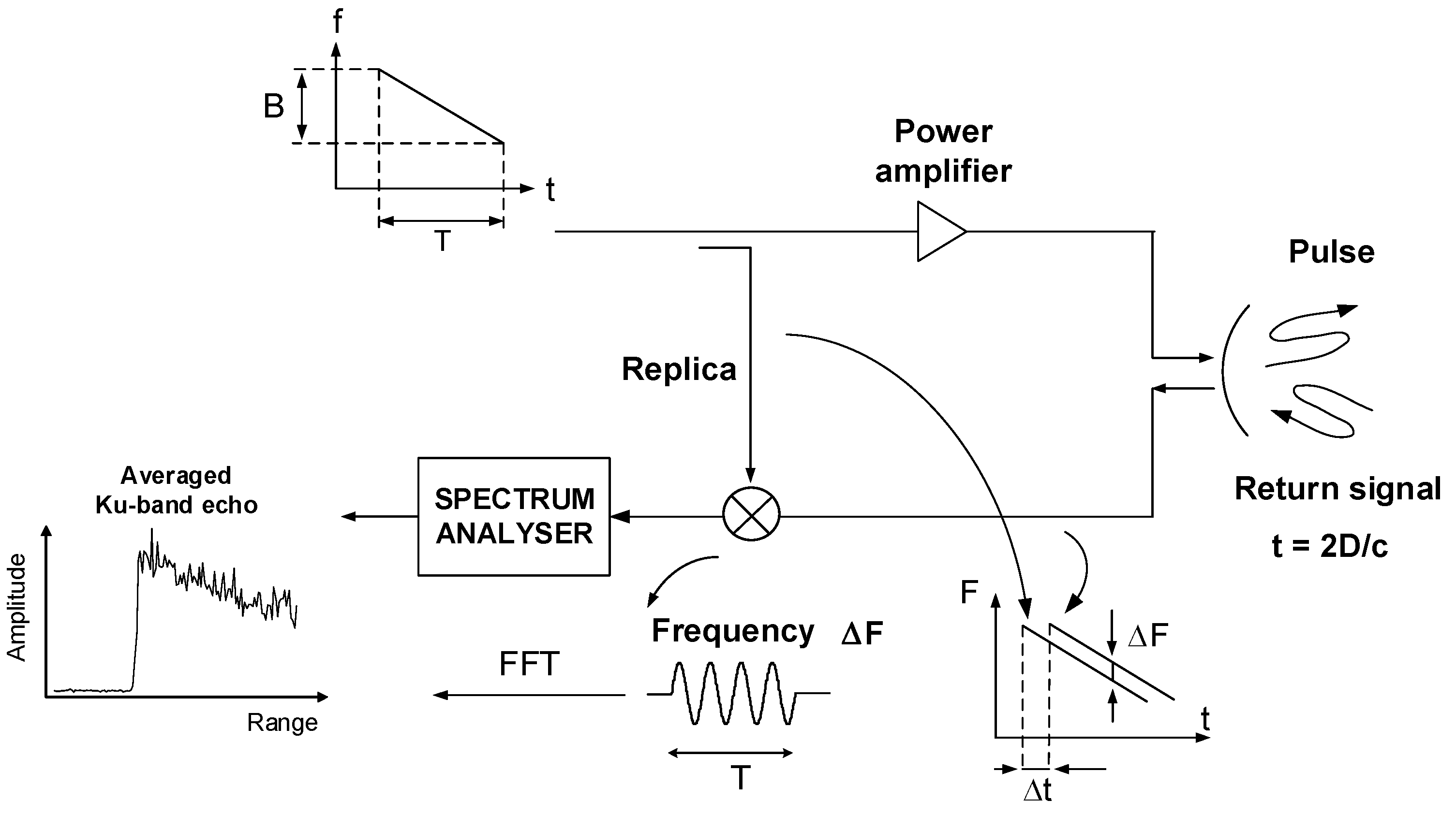
Figure 2.
POSEIDON-3C rough Ku band echoes measured over ocean on the 16th of January 2023 (Gates axis represents the range bins, Echoes axis represents each recorded echo and the vertical axis represents the amplitude of digitized echoes).
Figure 2.
POSEIDON-3C rough Ku band echoes measured over ocean on the 16th of January 2023 (Gates axis represents the range bins, Echoes axis represents each recorded echo and the vertical axis represents the amplitude of digitized echoes).
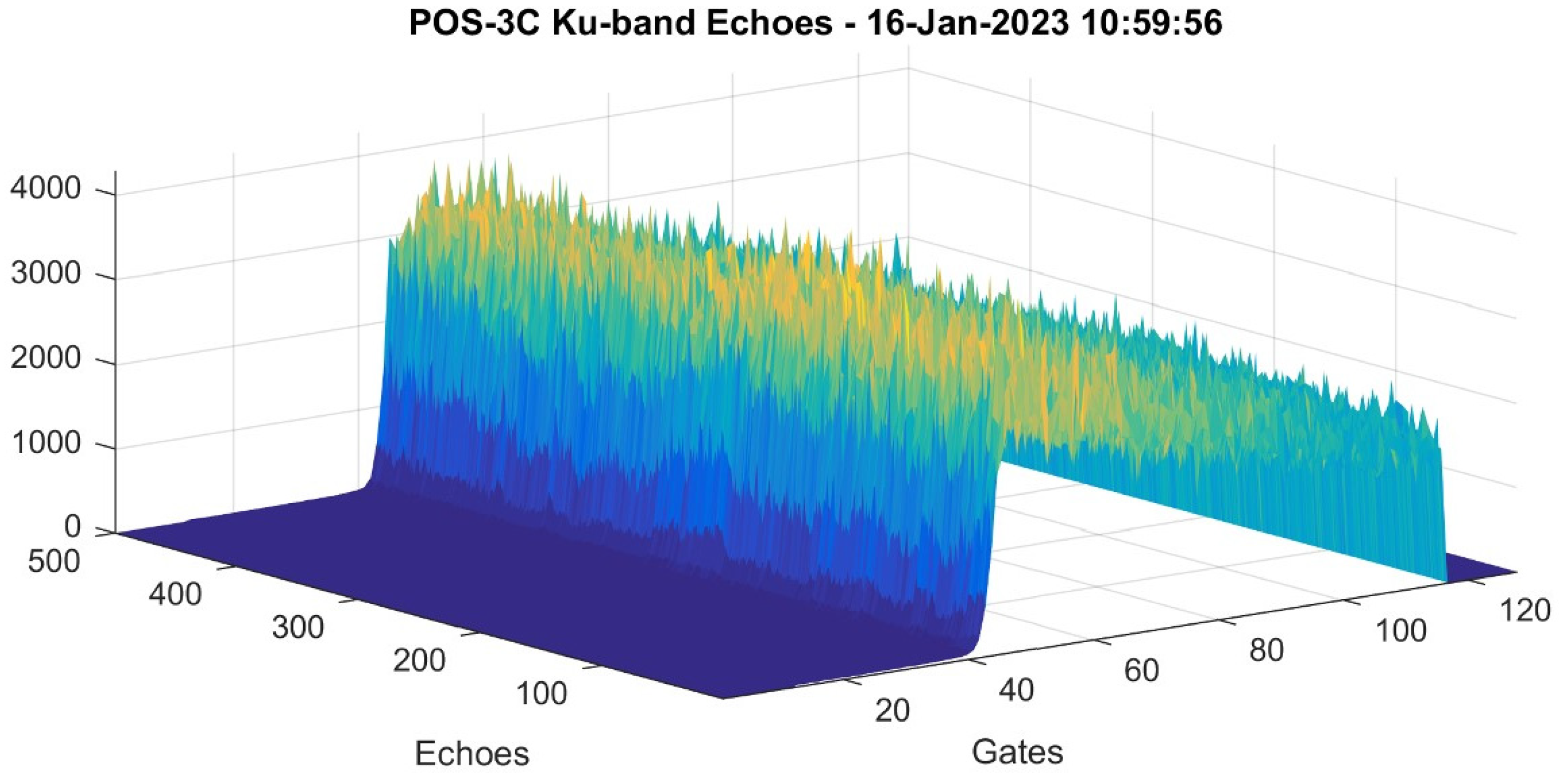
Figure 3.
(a) POSEIDON 3C architecture. The nadir altimeter is composed of an antenna, a radio frequency unit (RFU) and a processing and control unit (PCU); (b) RFU (right) and PCU (left) units on flight panel (credit: CNES and Thales Alenia Space); (c) Overall payload module with nadir dual frequency antenna (white reflector).
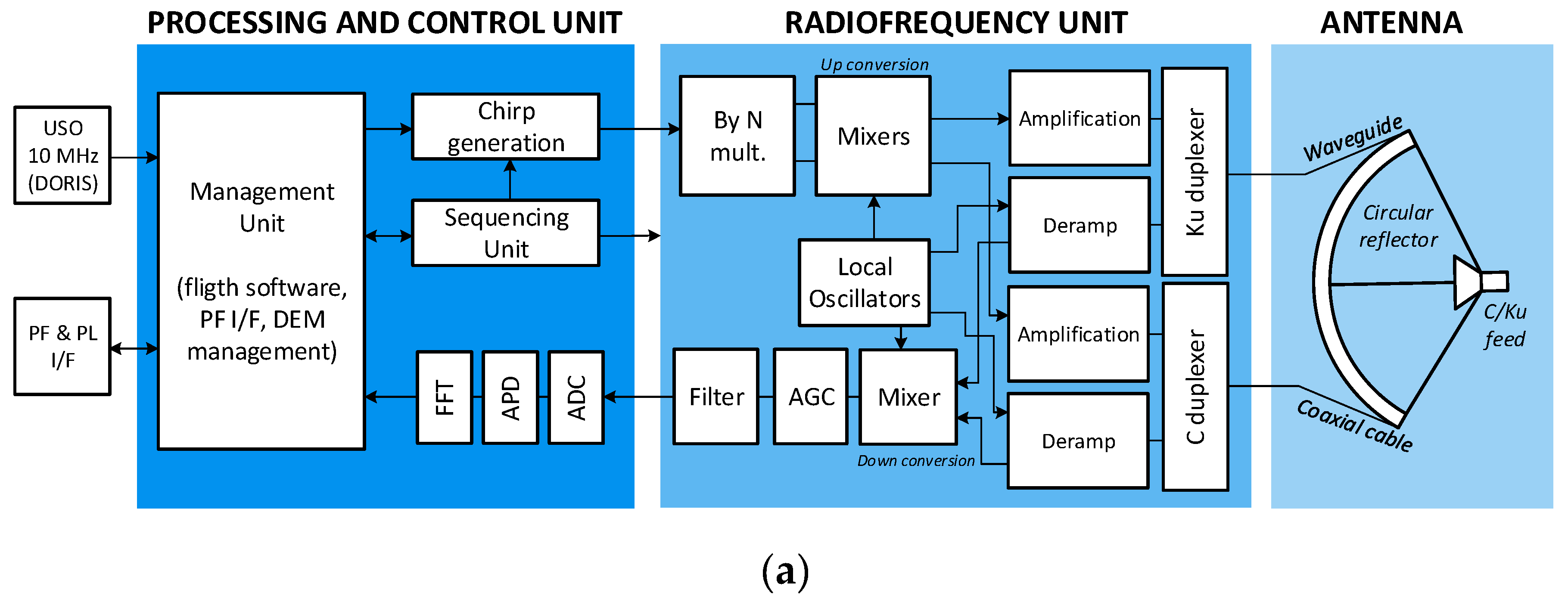
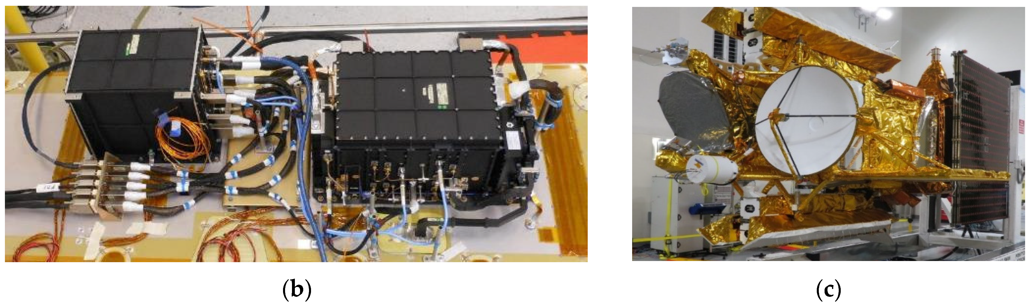
Figure 4.
POSEIDON-3C tracking modes transitions.
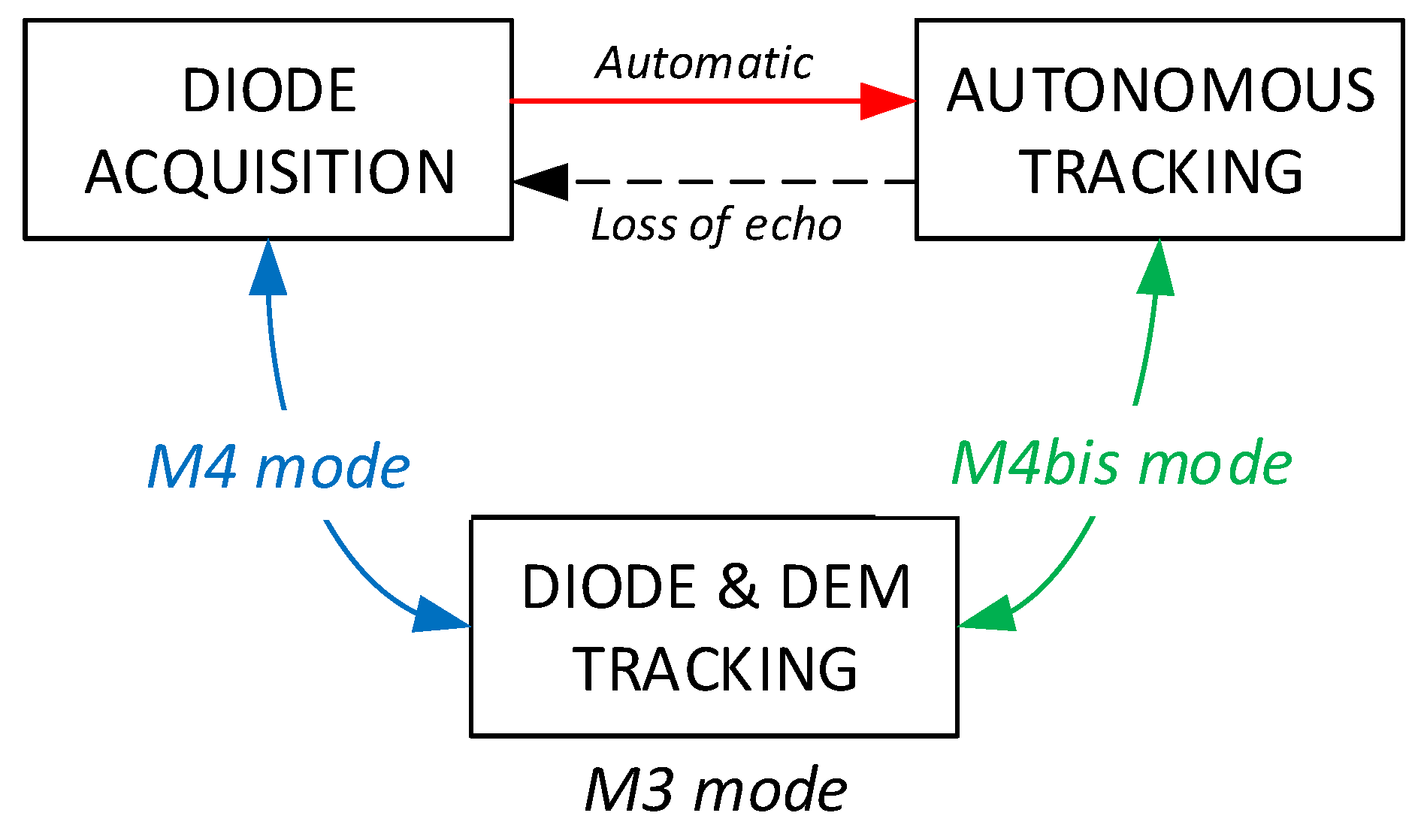
Figure 5.
Local repartition of the hydrological targets database for the SWOT 1-day orbit. The targets are colored by type as follows: LAK for lakes, RES for reservoirs, RIV for rivers.
Figure 5.
Local repartition of the hydrological targets database for the SWOT 1-day orbit. The targets are colored by type as follows: LAK for lakes, RES for reservoirs, RIV for rivers.
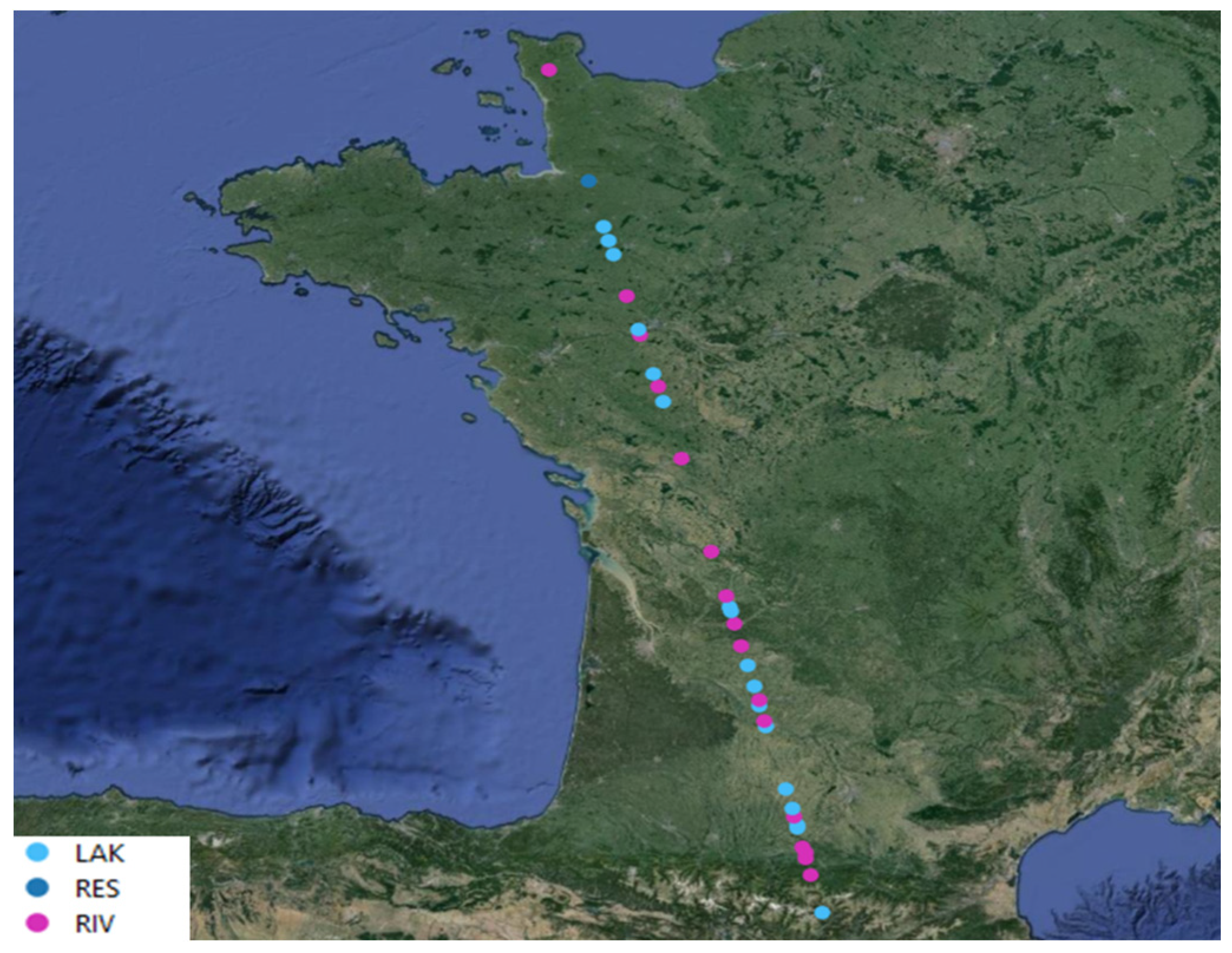
Figure 6.
Hydrological targets database for the SWOT 21-day Science orbit. The targets are colored by type: LAK for lakes (33741 targets, in light blue), RES for reservoirs (3239 targets, in blue), and RIV for rivers (21701, in magenta).
Figure 6.
Hydrological targets database for the SWOT 21-day Science orbit. The targets are colored by type: LAK for lakes (33741 targets, in light blue), RES for reservoirs (3239 targets, in blue), and RIV for rivers (21701, in magenta).
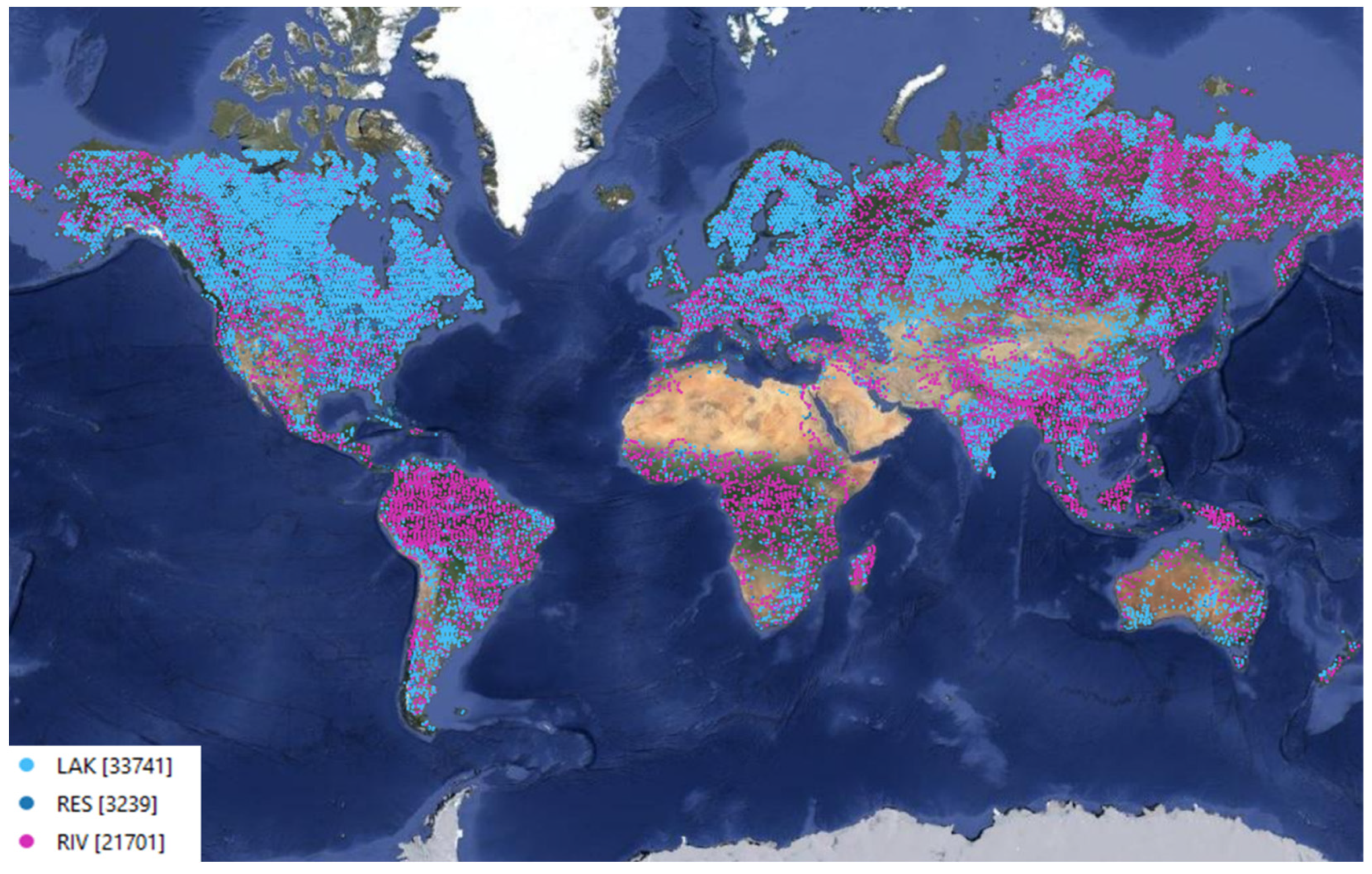
Figure 7.
(a) Histograms of Ku-band AGC in blue and C-band AGC in red; (b) Gridded maps (1°x1°) of Ku-band AGC; (c) Gridded maps (1°x1°) of C-band AGC.
Figure 7.
(a) Histograms of Ku-band AGC in blue and C-band AGC in red; (b) Gridded maps (1°x1°) of Ku-band AGC; (c) Gridded maps (1°x1°) of C-band AGC.
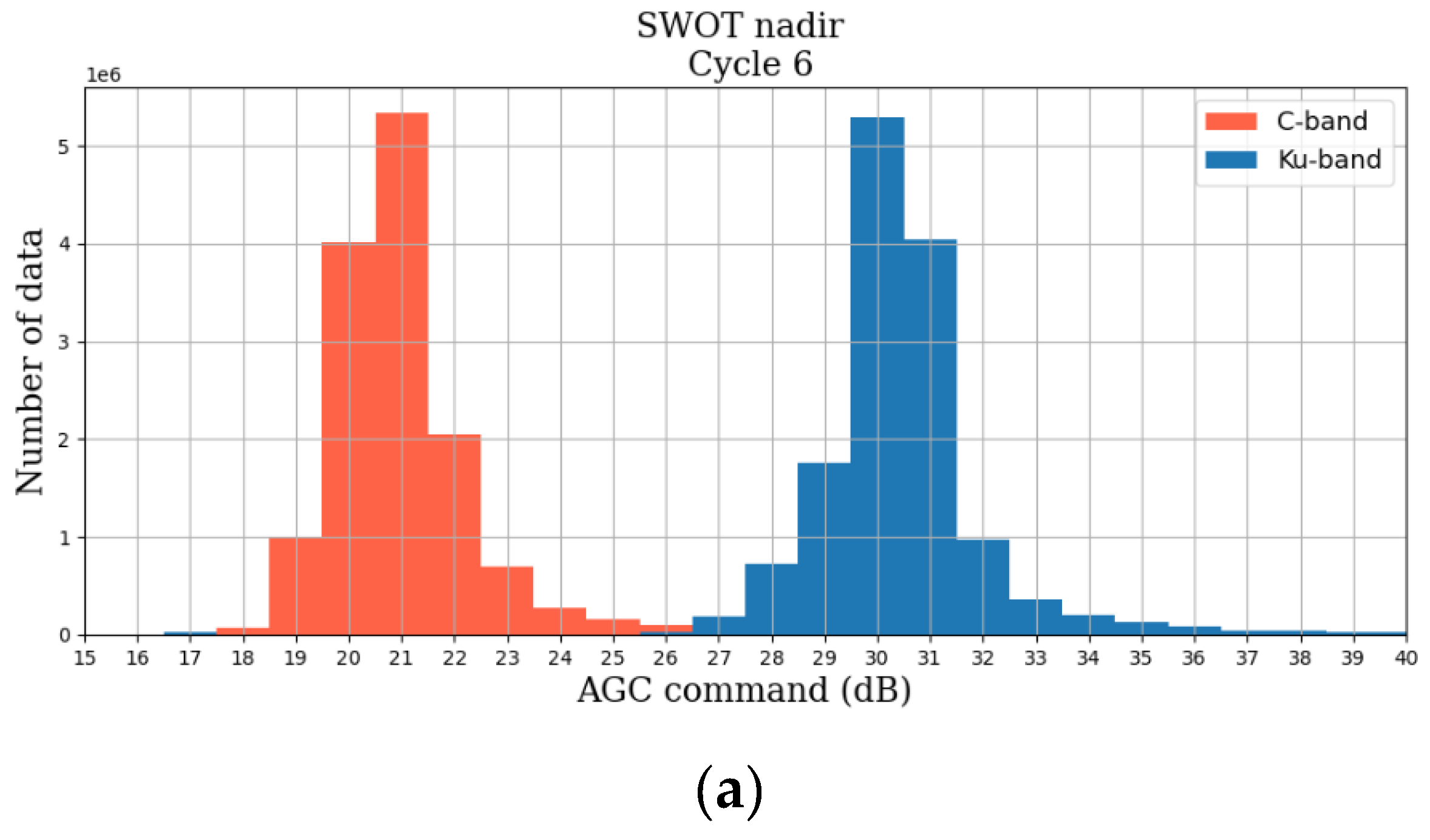
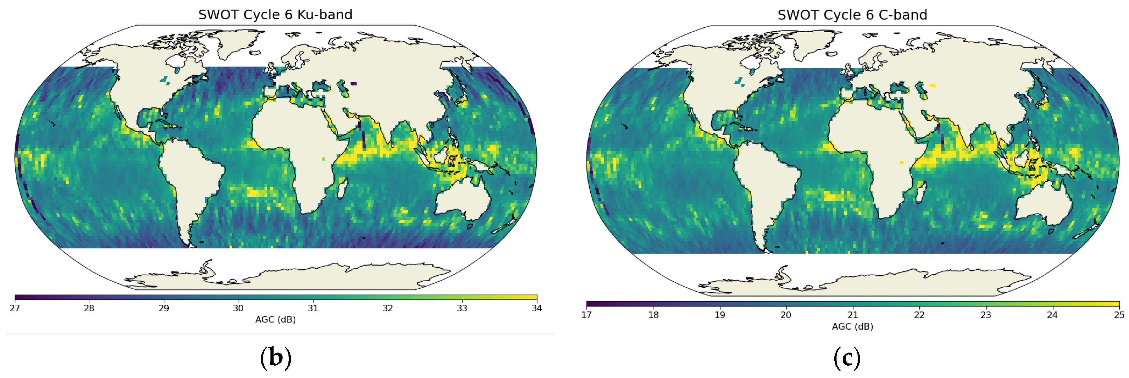
Figure 8.
(a) SWOT Gridded maps (1 × 1°) of Signal-to-Noise Ratio; (b) SWOT corresponding SNR histogram; (c) JASON-3 Gridded maps (1x1°) of Signal-to-Noise Ratio; (d) JASON-3 corresponding SNR histogram.
Figure 8.
(a) SWOT Gridded maps (1 × 1°) of Signal-to-Noise Ratio; (b) SWOT corresponding SNR histogram; (c) JASON-3 Gridded maps (1x1°) of Signal-to-Noise Ratio; (d) JASON-3 corresponding SNR histogram.
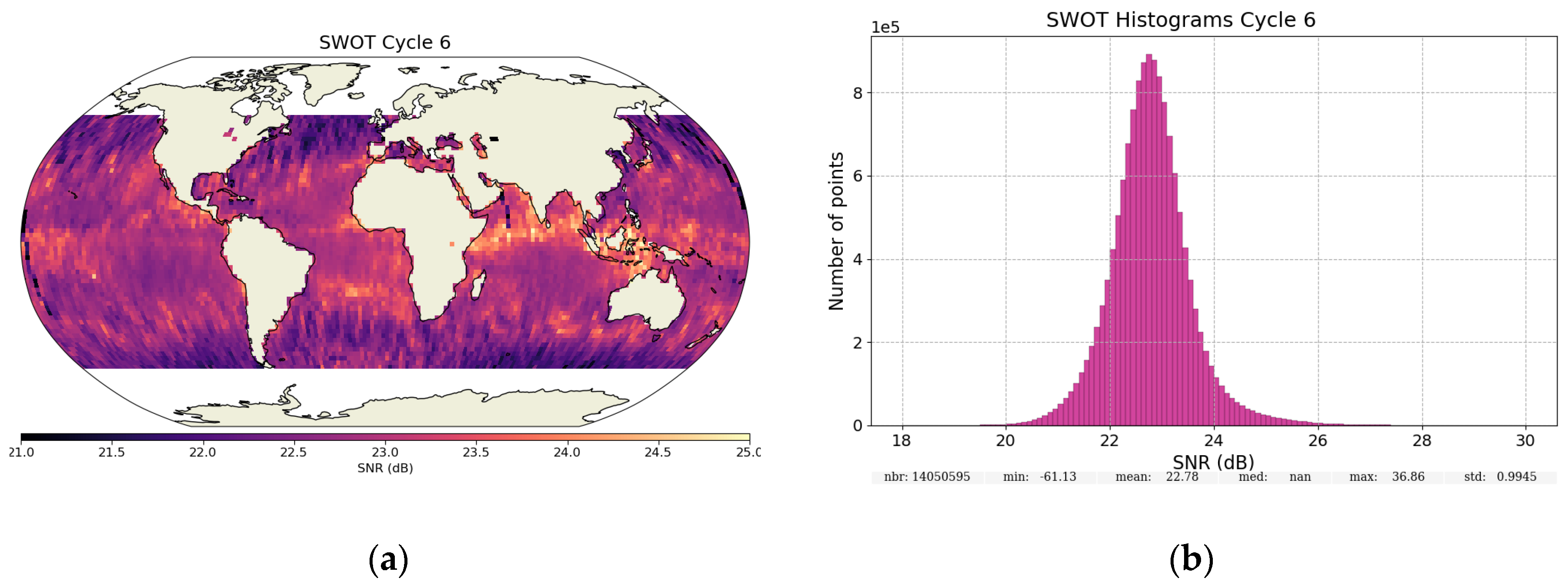
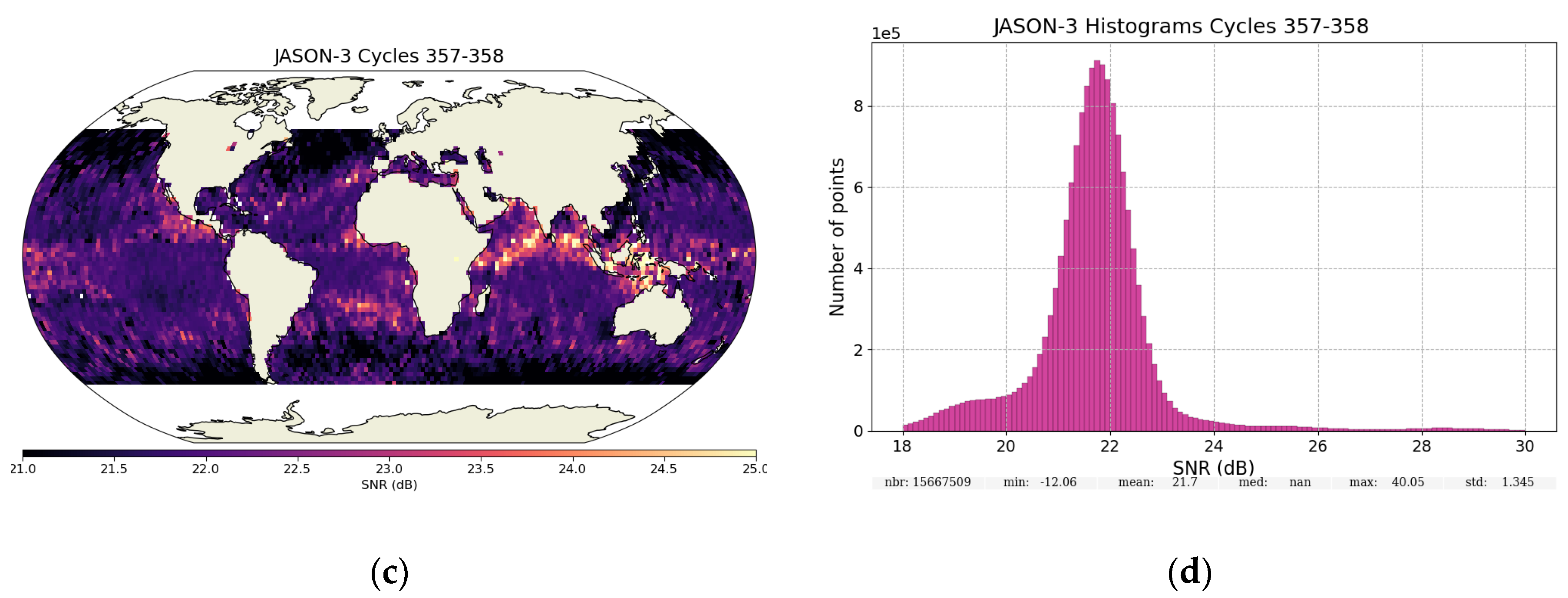
Figure 9.
Here the echo is represented only on the 104 useful gates, corresponding to gates [12:116] of the full analysis window. (a) Typical oceanic waveform for SWOT/POSEIDON-3C (blue) and JASON-3/POSEIDON-3B (red) for the full analysis window; (b) zoom on the first gates.
Figure 9.
Here the echo is represented only on the 104 useful gates, corresponding to gates [12:116] of the full analysis window. (a) Typical oceanic waveform for SWOT/POSEIDON-3C (blue) and JASON-3/POSEIDON-3B (red) for the full analysis window; (b) zoom on the first gates.
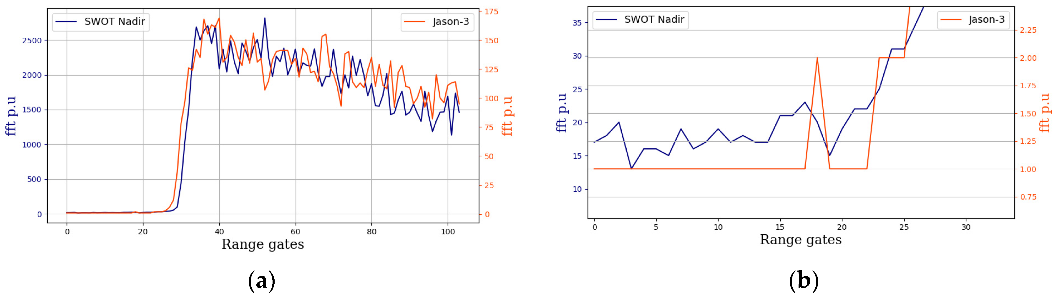
Figure 10.
Example of automatic transitions between Open-loop and Closed-loop tracking modes over land areas.
Figure 10.
Example of automatic transitions between Open-loop and Closed-loop tracking modes over land areas.
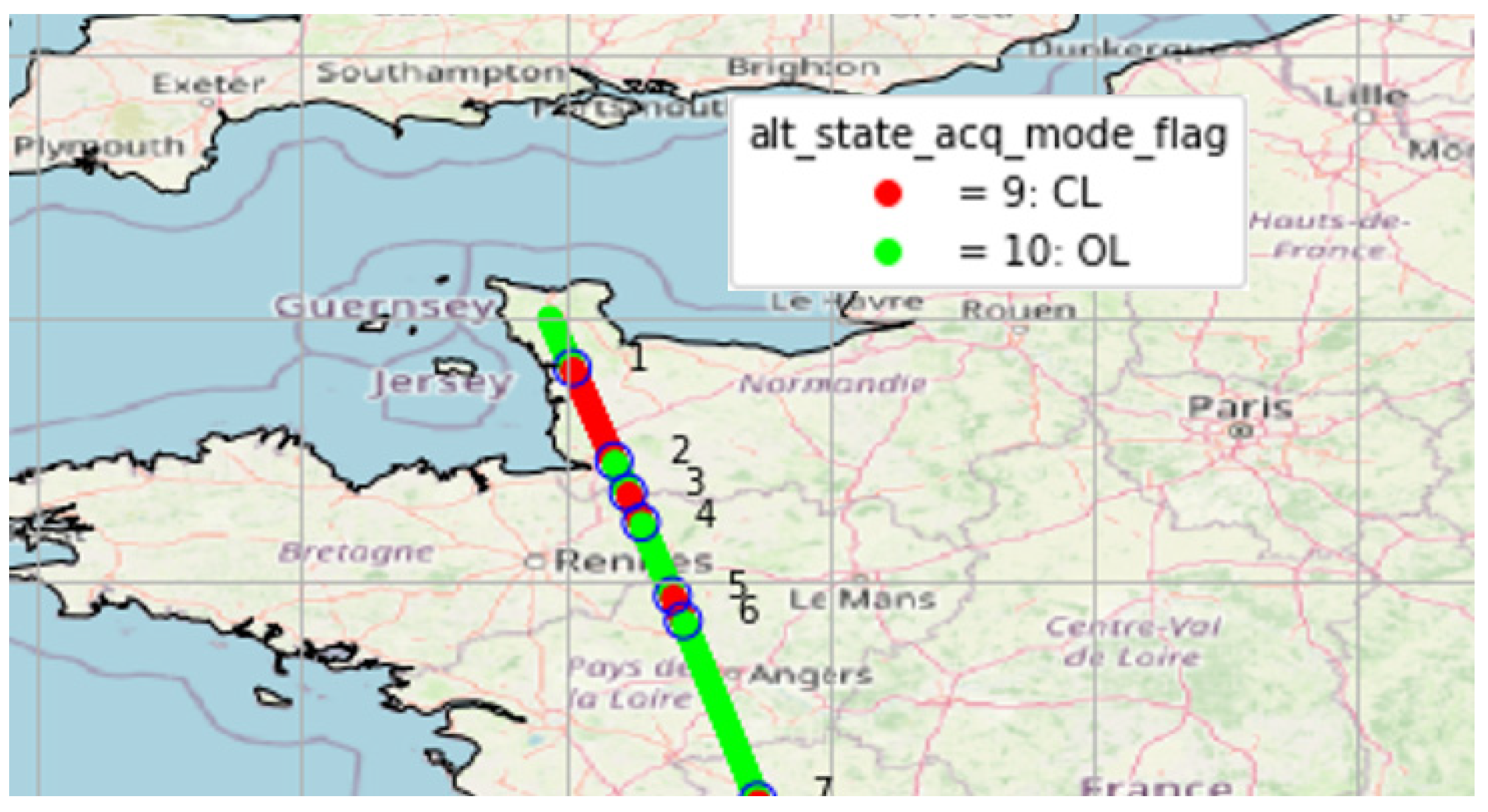
Figure 11.
Example of an Open-Loop to Closed-Loop transition, acquired under M4 mode (left, cycle 447) and M4bis mode (right, cycle 470). The mode mask from the OLTC is shown at the bottom of each graph: green for OL, and red for CL. On top of the graphs, the effective pursuit mode of SWOT is shown as read in the Level-2 products.
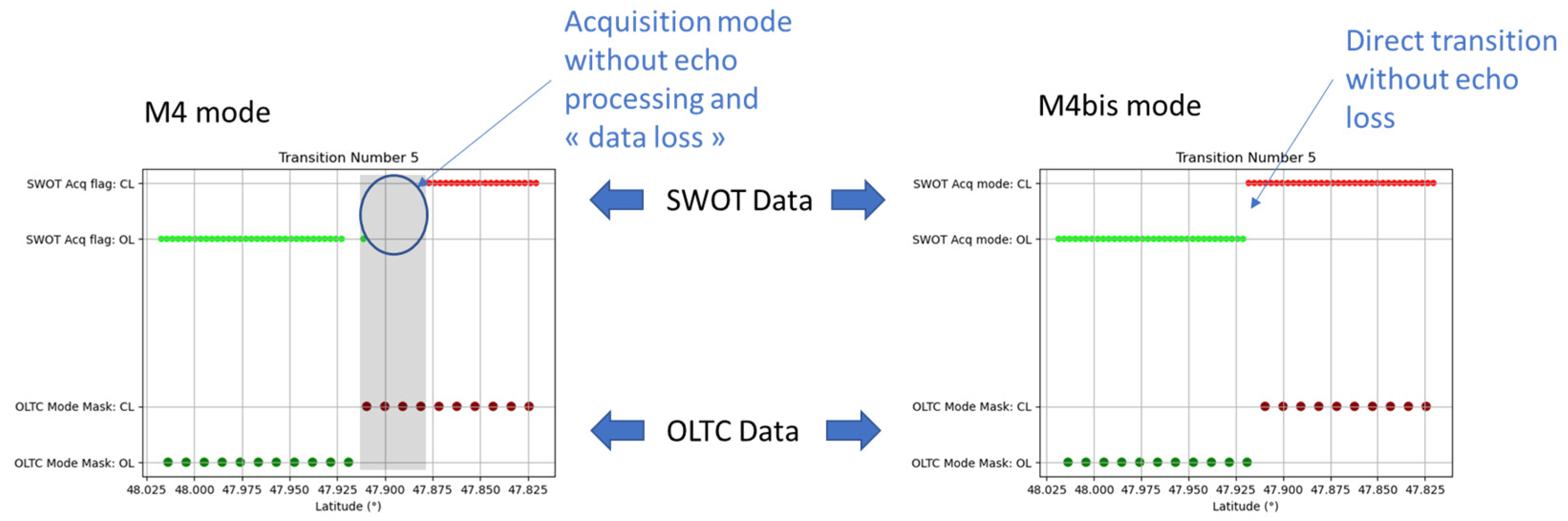
Figure 12.
Examples of radargrams at the transition between the Atlantic Ocean and Suriname (Descending Pass 464) for the closed-loop (left panel) and the open-loop (right panel), represented on Google Earth. The orange arrow represents the satellite’s tracking direction.
Figure 12.
Examples of radargrams at the transition between the Atlantic Ocean and Suriname (Descending Pass 464) for the closed-loop (left panel) and the open-loop (right panel), represented on Google Earth. The orange arrow represents the satellite’s tracking direction.
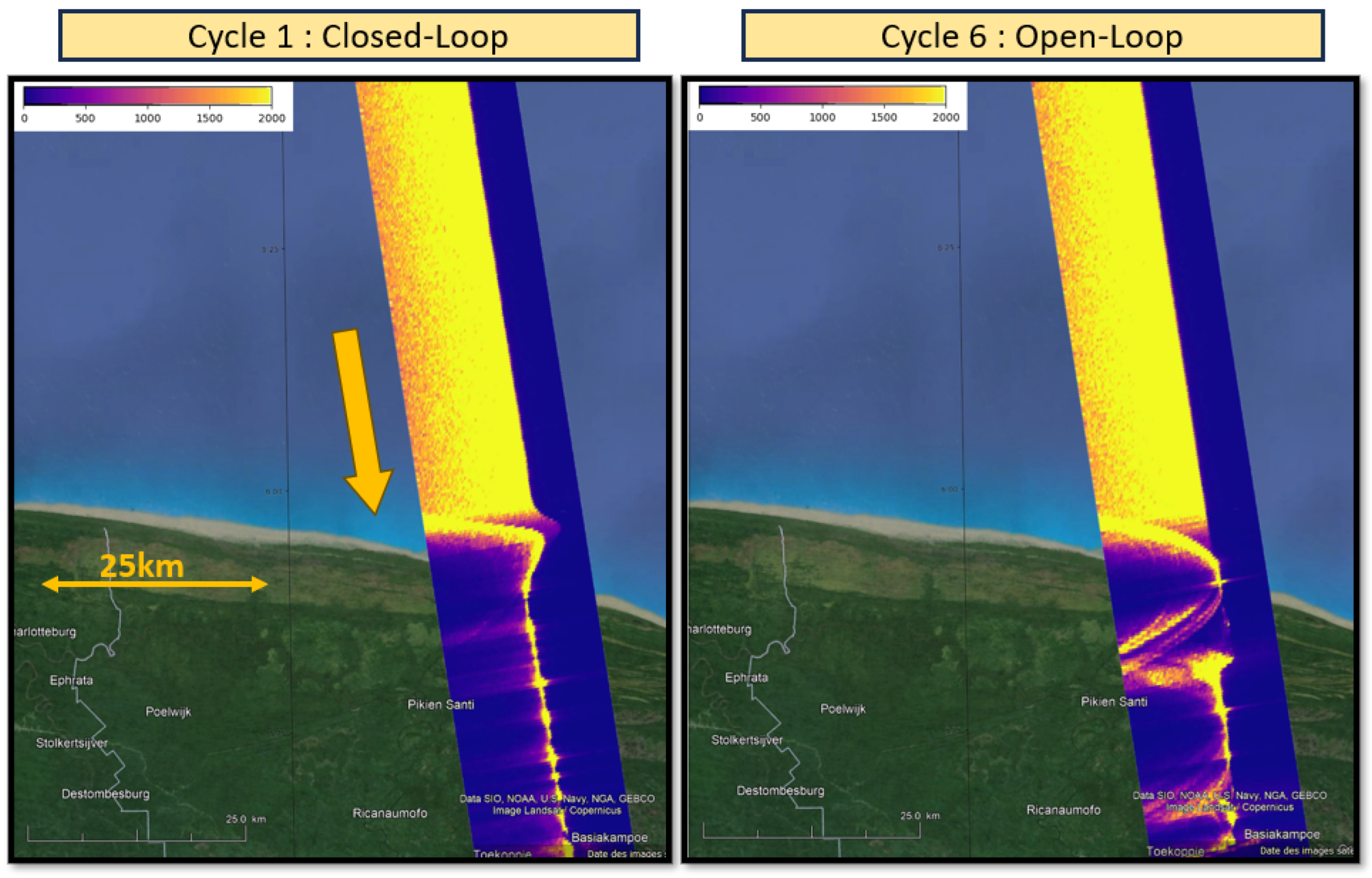
Figure 13.
Examples of radargrams at the transition between Spain and the Atlantic Ocean (Ascending Pass 475) for the closed-loop (left panel) and the open-loop (right panel), represented on Google Earth. The orange arrow represents the satellite’s tracking direction.
Figure 13.
Examples of radargrams at the transition between Spain and the Atlantic Ocean (Ascending Pass 475) for the closed-loop (left panel) and the open-loop (right panel), represented on Google Earth. The orange arrow represents the satellite’s tracking direction.
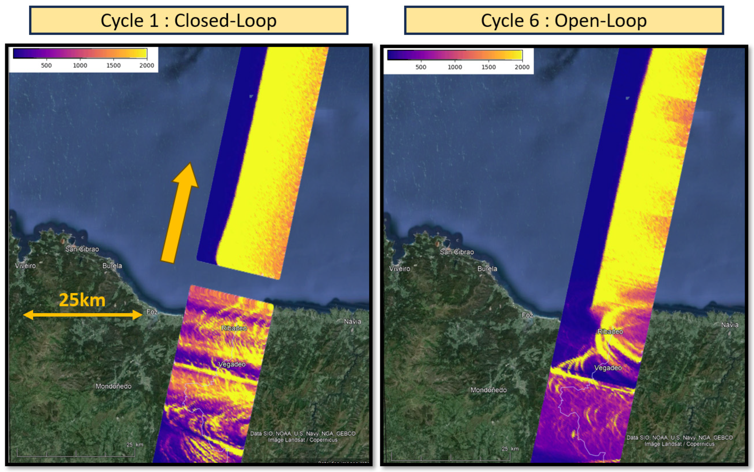
Figure 14.
(a) Example of a saturated waveform zoomed around the peak; (b) location of all saturated waveforms over cycle 6 of SWOT nadir.
Figure 14.
(a) Example of a saturated waveform zoomed around the peak; (b) location of all saturated waveforms over cycle 6 of SWOT nadir.
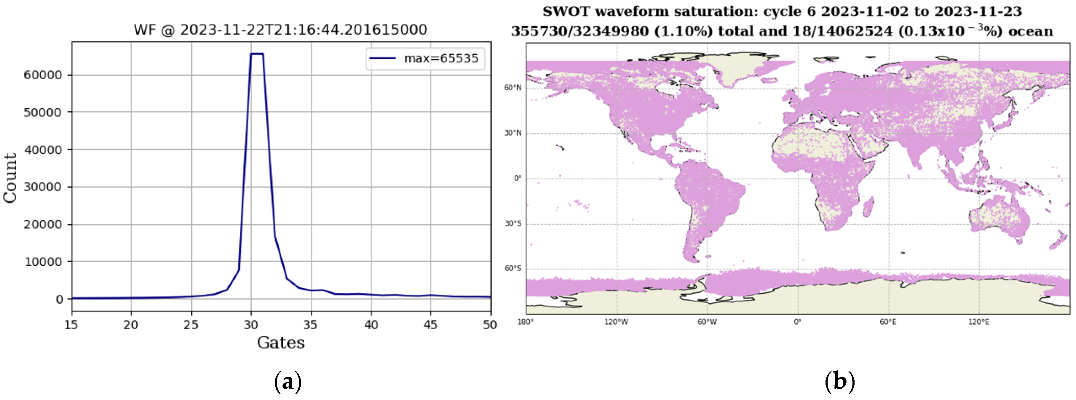
Figure 15.
Locations of the routine CAL1 & CAL2 calibrations delimited by red rectangles.
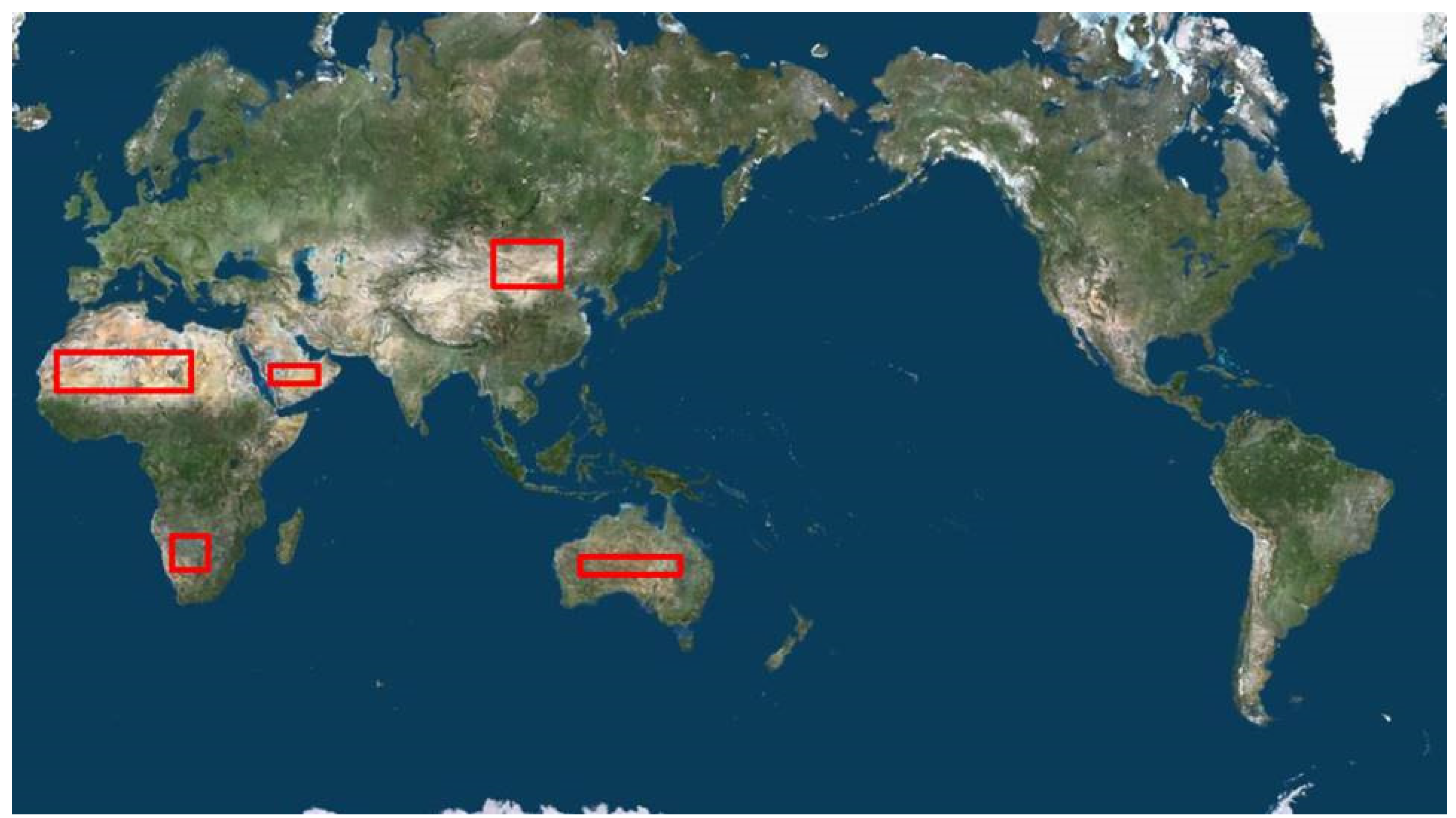
Figure 16.
Time-series of the in-orbit temperatures (in °C) for the RFU SSPA board, RFU Rx board and PCU DC/DC board in Ku-band (in blue), averaged over a 1-day sliding window. In orange is the sun beta prime angle.
Figure 16.
Time-series of the in-orbit temperatures (in °C) for the RFU SSPA board, RFU Rx board and PCU DC/DC board in Ku-band (in blue), averaged over a 1-day sliding window. In orange is the sun beta prime angle.
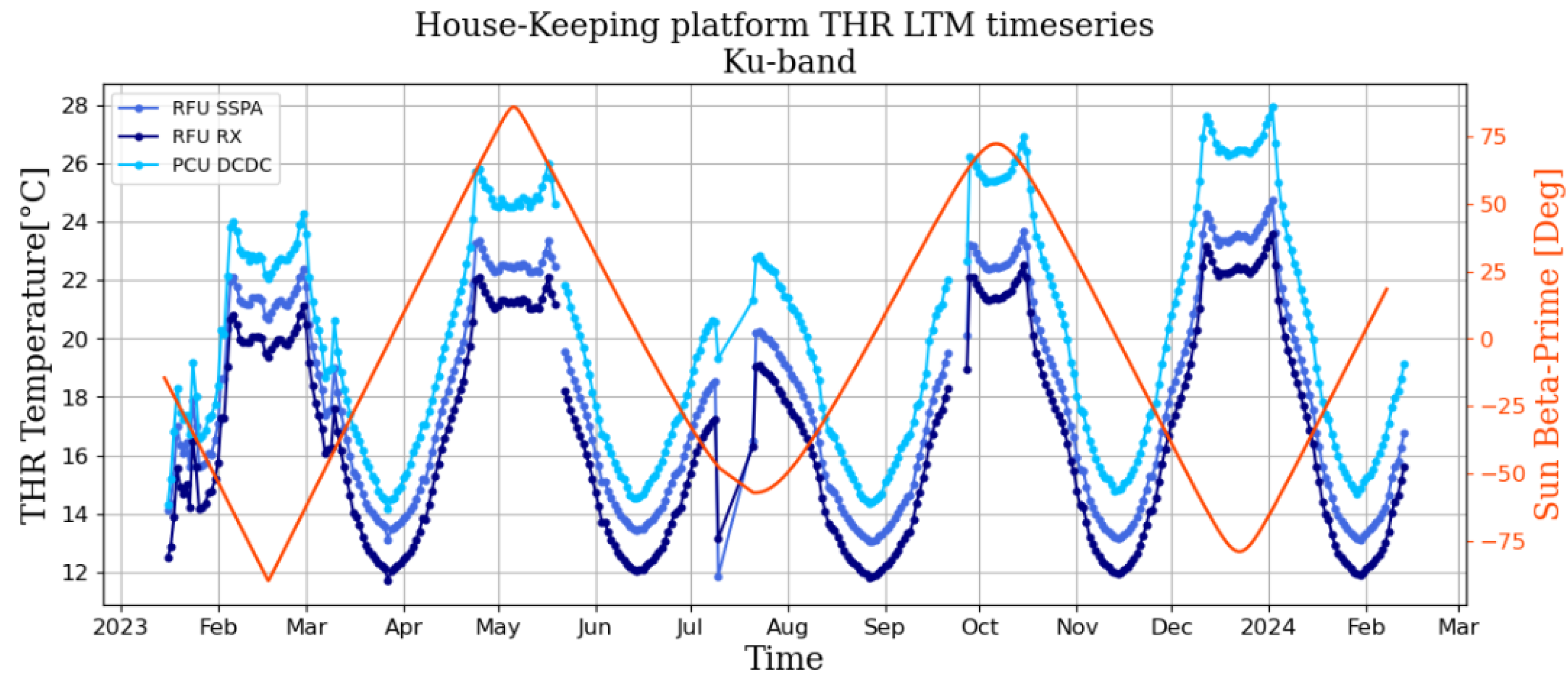
Figure 17.
Time-series of the in-orbit temperatures (in °C) for the RFU SSPA and Rx boards in C-band (in blue), averaged over a 1-day sliding window. In orange is the sun beta prime angle.
Figure 17.
Time-series of the in-orbit temperatures (in °C) for the RFU SSPA and Rx boards in C-band (in blue), averaged over a 1-day sliding window. In orange is the sun beta prime angle.
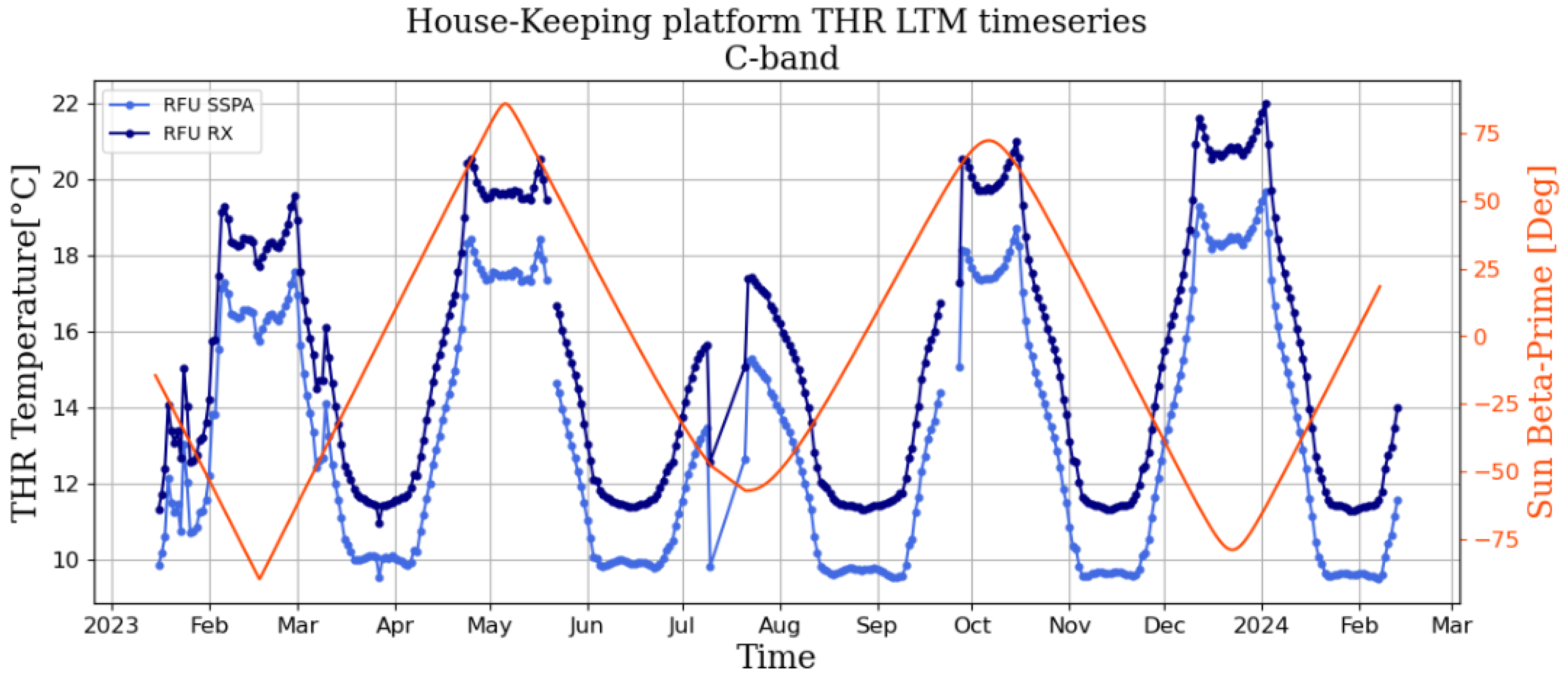
Figure 18.
Example of an In-flight CAL1 in blue compared to perfect sinc2 corrected from the internal path delay (in red) for the Ku-band (top panel) and the C-band (bottom panel). The orange dashed line represents the center of the receiving window (0-frequency).
Figure 18.
Example of an In-flight CAL1 in blue compared to perfect sinc2 corrected from the internal path delay (in red) for the Ku-band (top panel) and the C-band (bottom panel). The orange dashed line represents the center of the receiving window (0-frequency).
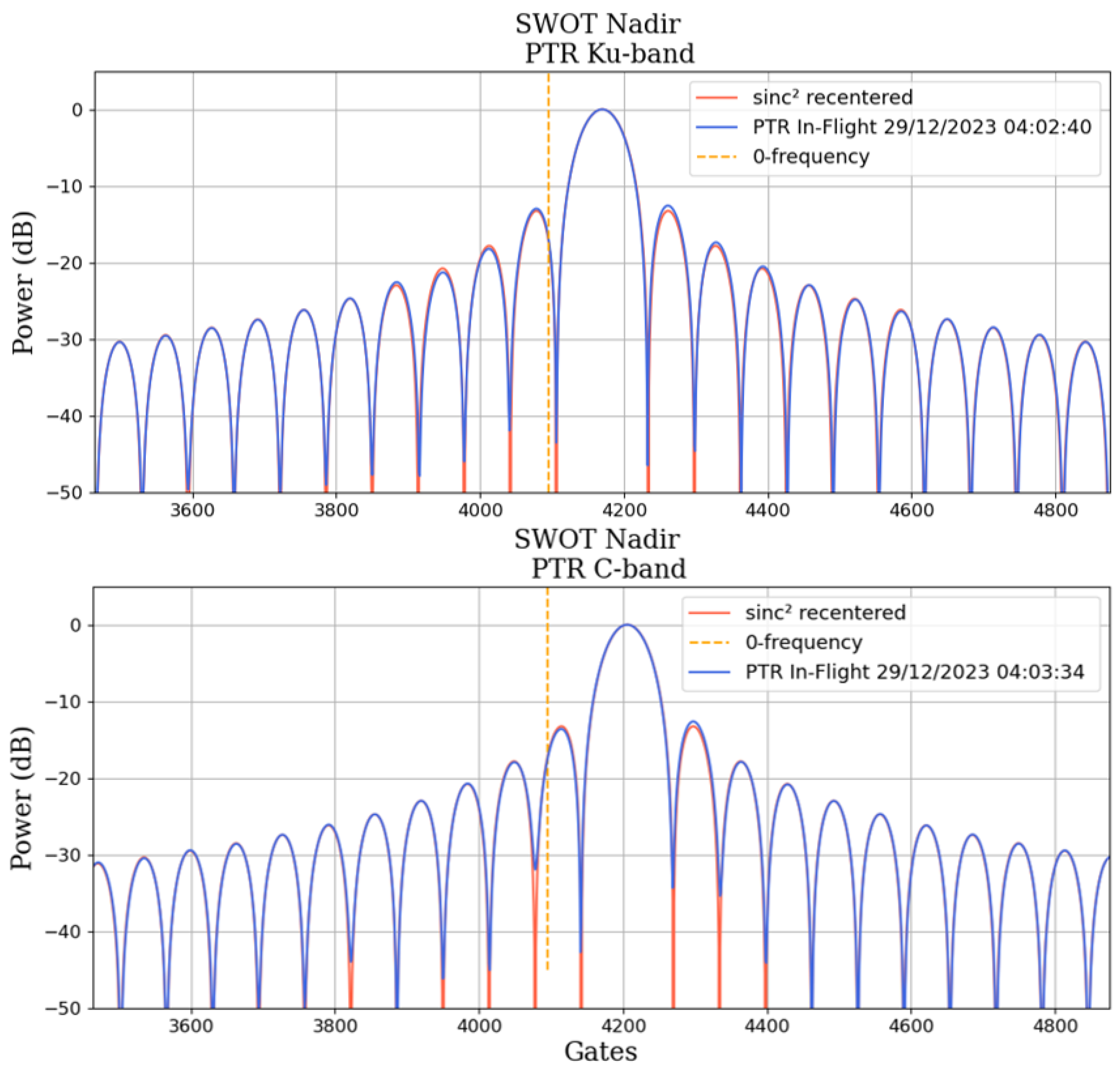
Figure 19.
Long-term monitoring of the PTR IPD, Total Power and WML for the Ku-band since altimeter switch-on. The SSPA House-Keeping temperatures is represented in grey in the secondary y-axis.
Figure 19.
Long-term monitoring of the PTR IPD, Total Power and WML for the Ku-band since altimeter switch-on. The SSPA House-Keeping temperatures is represented in grey in the secondary y-axis.
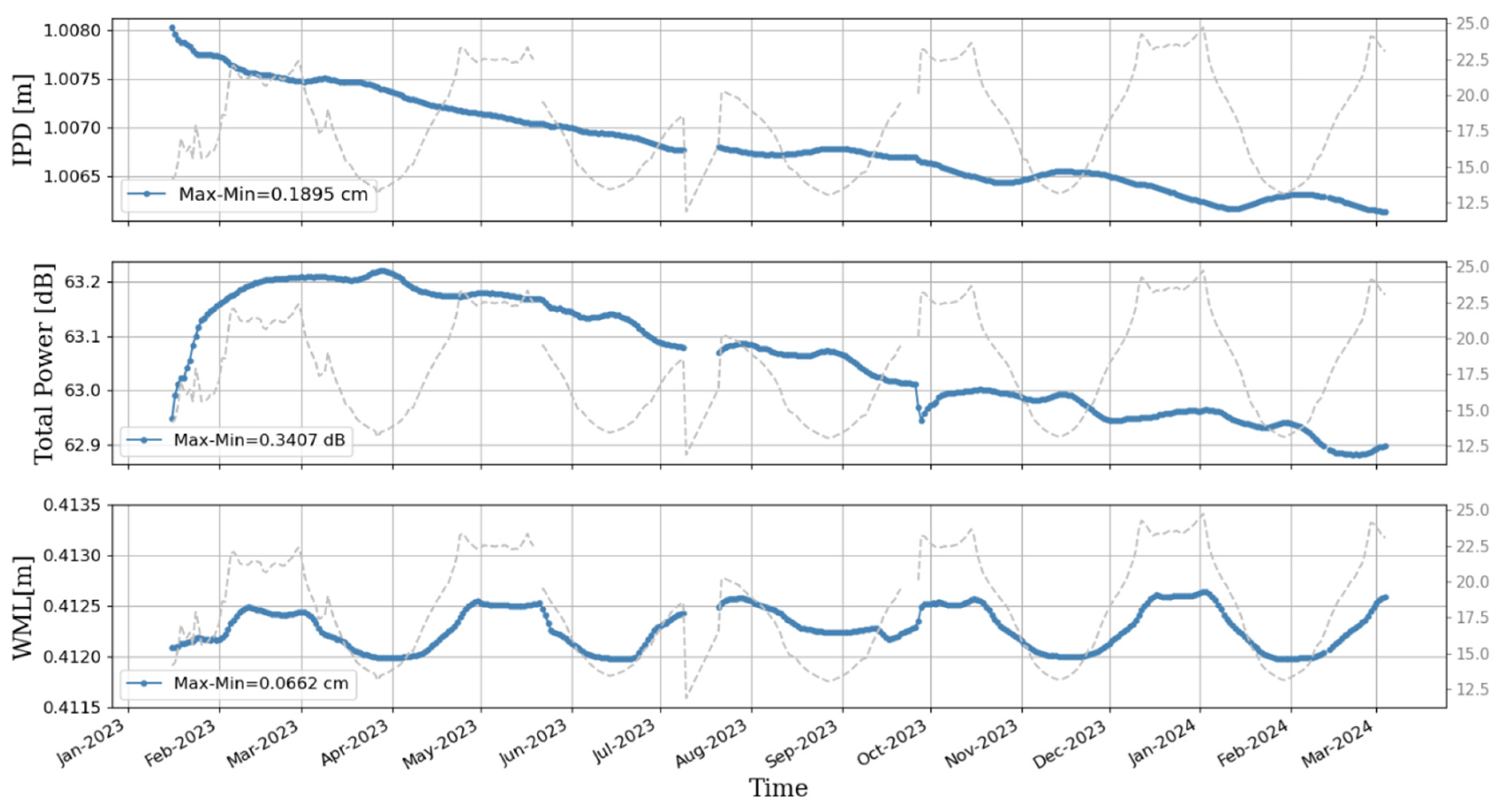
Figure 20.
Long-term monitoring of the PTR IPD, Total power and WML for the C-band since altimeter switch-on. The SSPA House-Keeping temperatures is represented in grey in the secondary y-axis.
Figure 20.
Long-term monitoring of the PTR IPD, Total power and WML for the C-band since altimeter switch-on. The SSPA House-Keeping temperatures is represented in grey in the secondary y-axis.
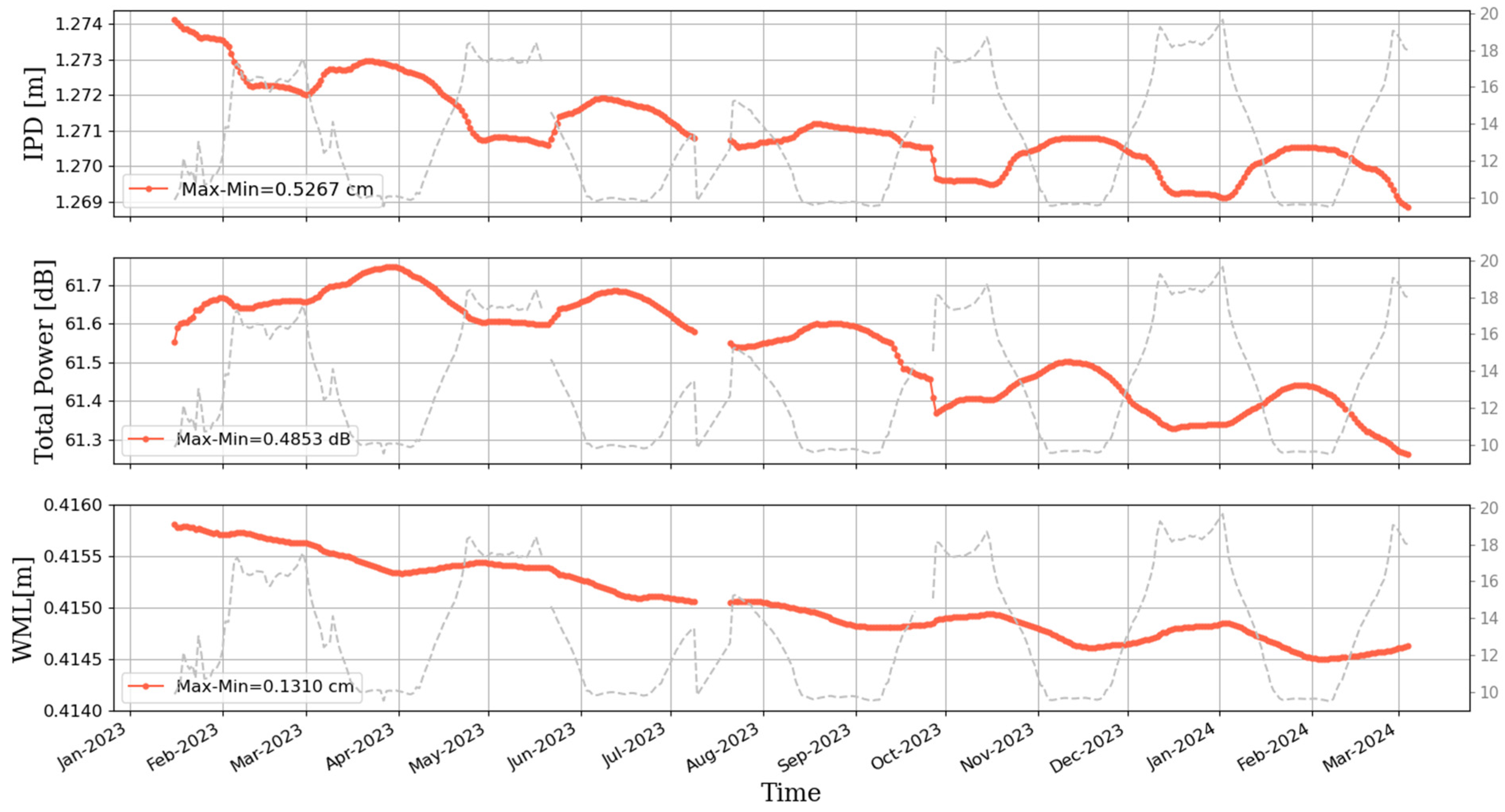
Figure 21.
Time series of the evolution of the first 5 sidelobes peak position (in meters) of the Ku-band PTR: (a) for the left-hand side; (b) for the right-hand side.
Figure 21.
Time series of the evolution of the first 5 sidelobes peak position (in meters) of the Ku-band PTR: (a) for the left-hand side; (b) for the right-hand side.
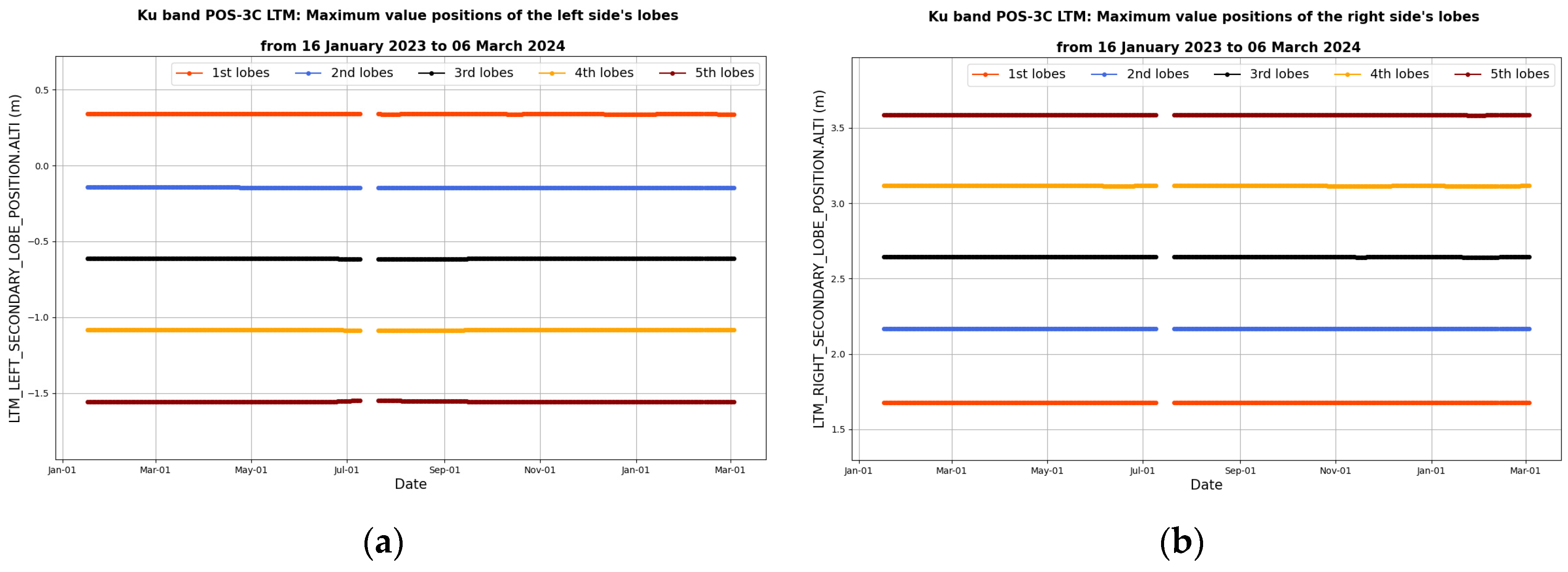
Figure 22.
Time series of the evolution of the first 5 sidelobes peak power (in dB) of the Ku-band PTR: (a) for the left-hand side; (b) for the right-hand side.
Figure 22.
Time series of the evolution of the first 5 sidelobes peak power (in dB) of the Ku-band PTR: (a) for the left-hand side; (b) for the right-hand side.
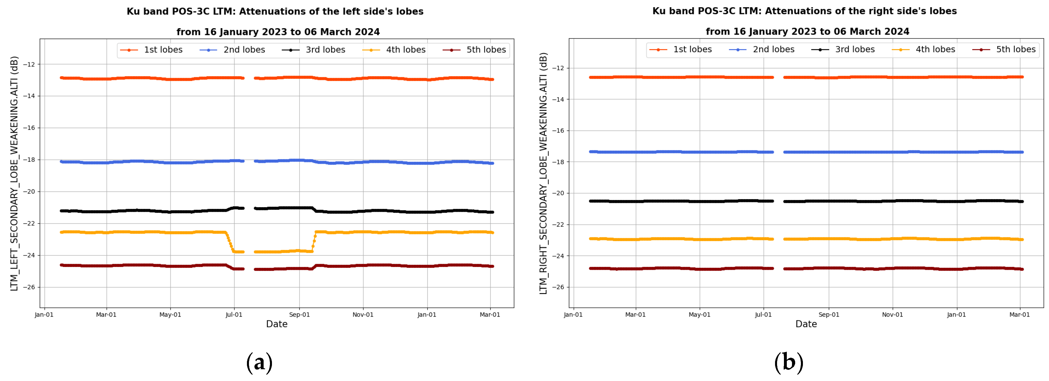
Figure 23.
(a) Time series of the difference in peak position between the first 5 sidelobes on the right-hand side and the left-hand side, for the Ku-band PTR. (b) Time series of the difference in peak power between the first 5 sidelobes on the right-hand side and the left-hand side, for the Ku-band PTR.
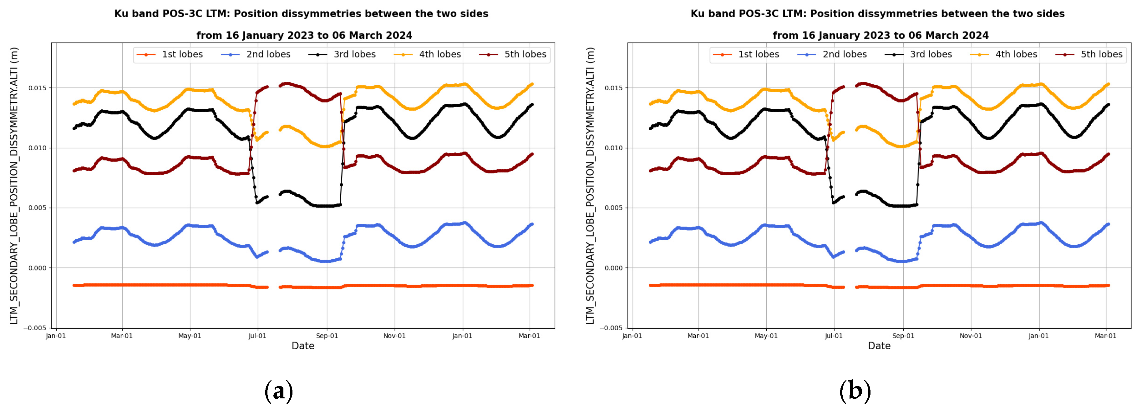
Figure 24.
Example of measured LPF in blue, compared to the ground calibrations in red: for the Ku-band (a) and the C-band (b). Top panel represents the full 128-gates window and bottom panel focuses on the useful 104-gates.
Figure 24.
Example of measured LPF in blue, compared to the ground calibrations in red: for the Ku-band (a) and the C-band (b). Top panel represents the full 128-gates window and bottom panel focuses on the useful 104-gates.
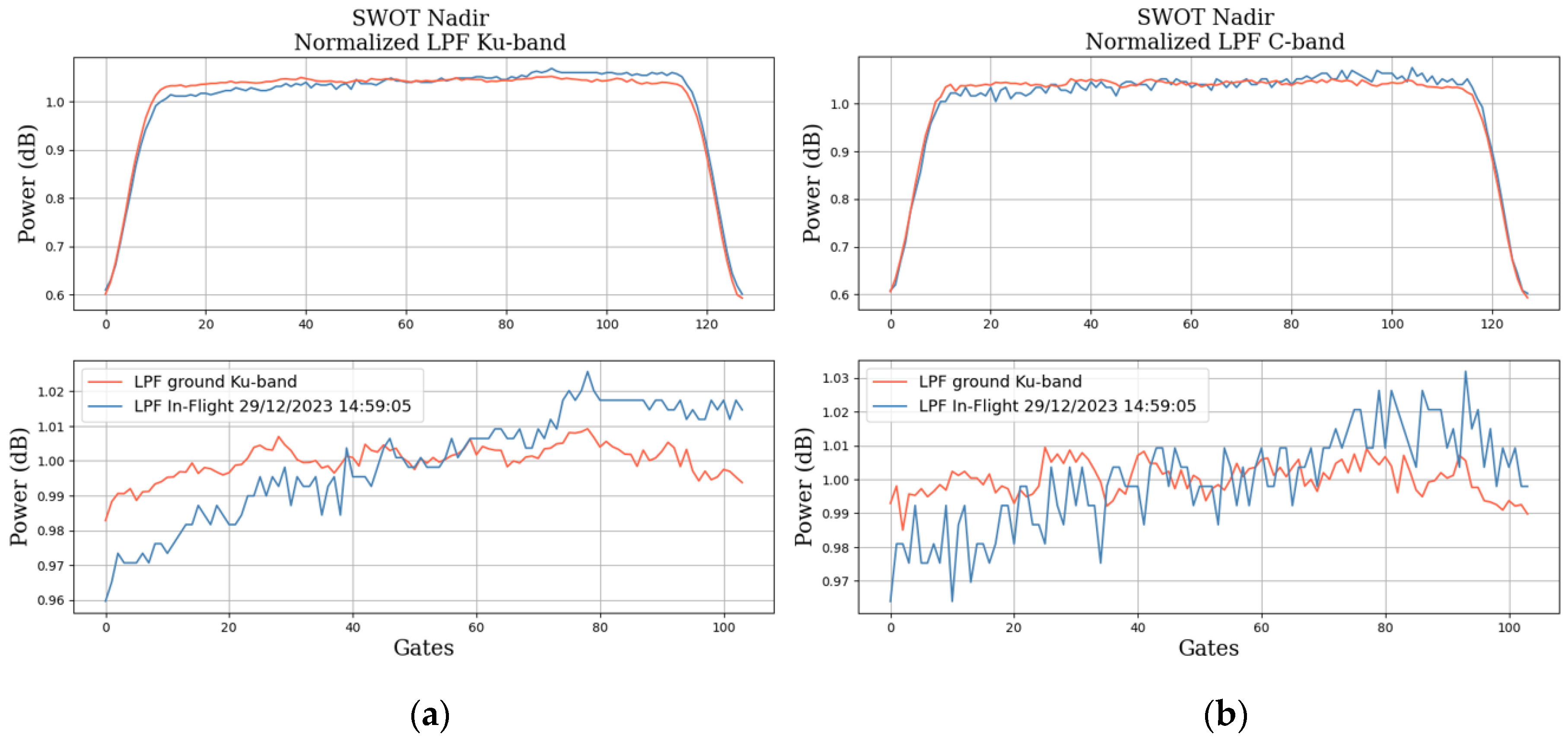
Figure 25.
(a)Time series of the LPF standard deviation [dB] in black, slope [dB/104-gates] in blue and ripple [dB]. (b) Time series of the full normalized 128-gates LPF. Top panel represents the Ku-band and bottom panel represents the C-band.
Figure 25.
(a)Time series of the LPF standard deviation [dB] in black, slope [dB/104-gates] in blue and ripple [dB]. (b) Time series of the full normalized 128-gates LPF. Top panel represents the Ku-band and bottom panel represents the C-band.
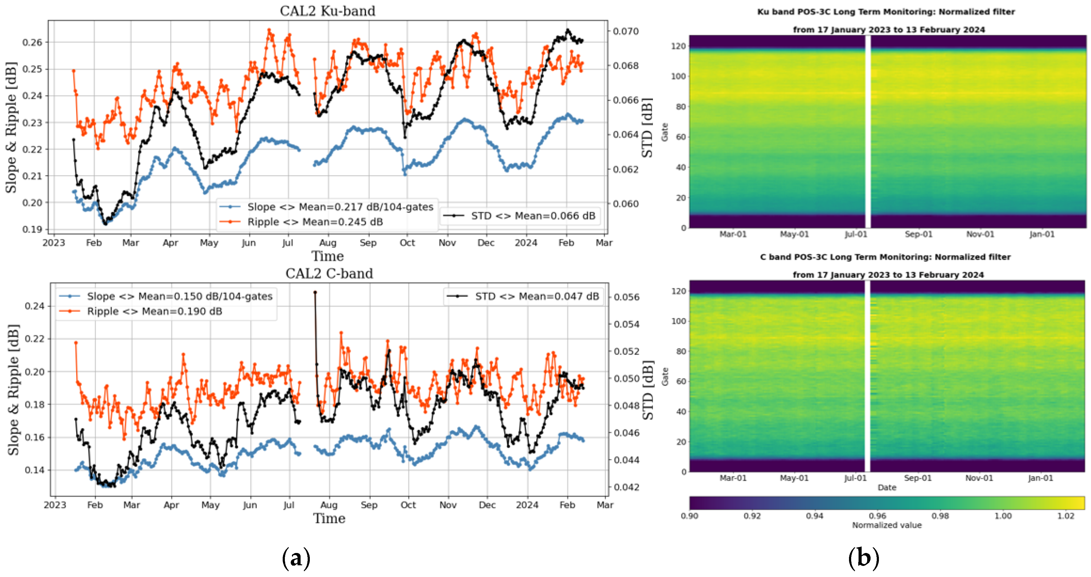
Figure 26.
Localization of the Point Target Response measurements performed to calibrate the Automatic Gain Control on September 9, 2023.
Figure 26.
Localization of the Point Target Response measurements performed to calibrate the Automatic Gain Control on September 9, 2023.
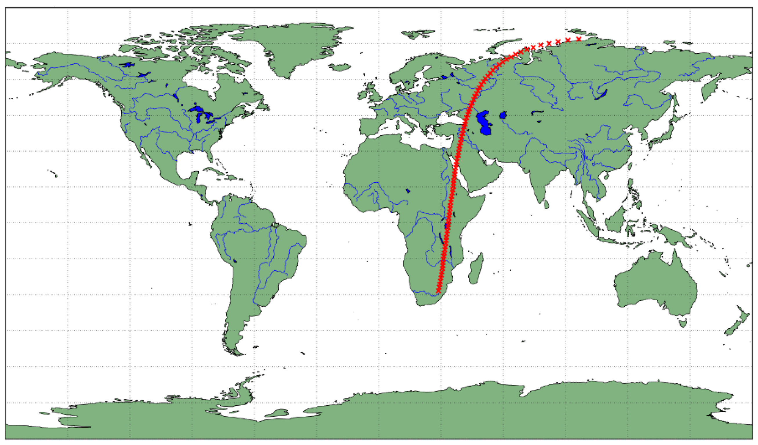
Figure 27.
Difference between actual and theoretical POSEIDONC-3C AGC values since SWOT launch.
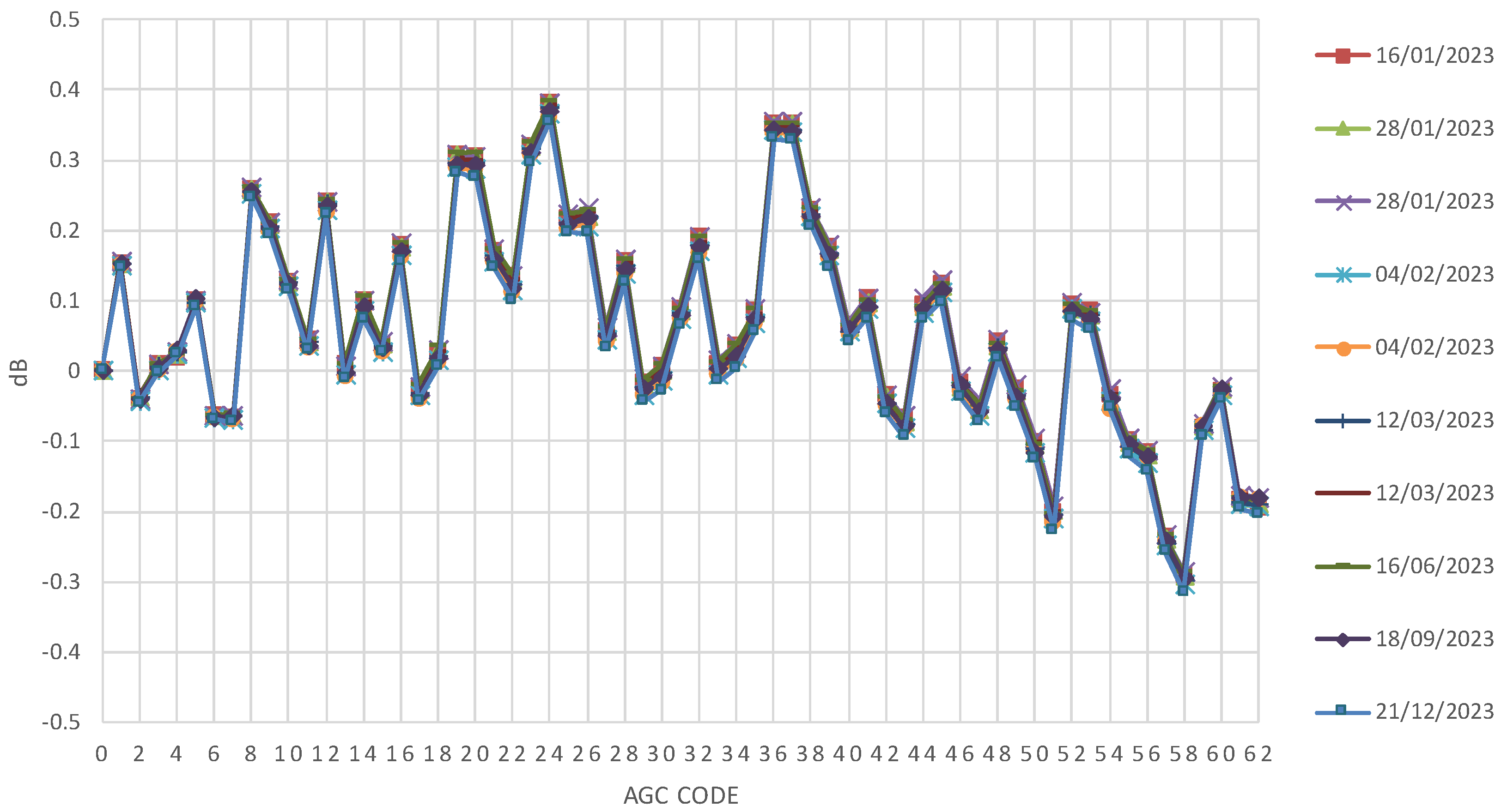
Figure 28.
Localization of the exceptional PTR measurements to assess in-orbit stability.
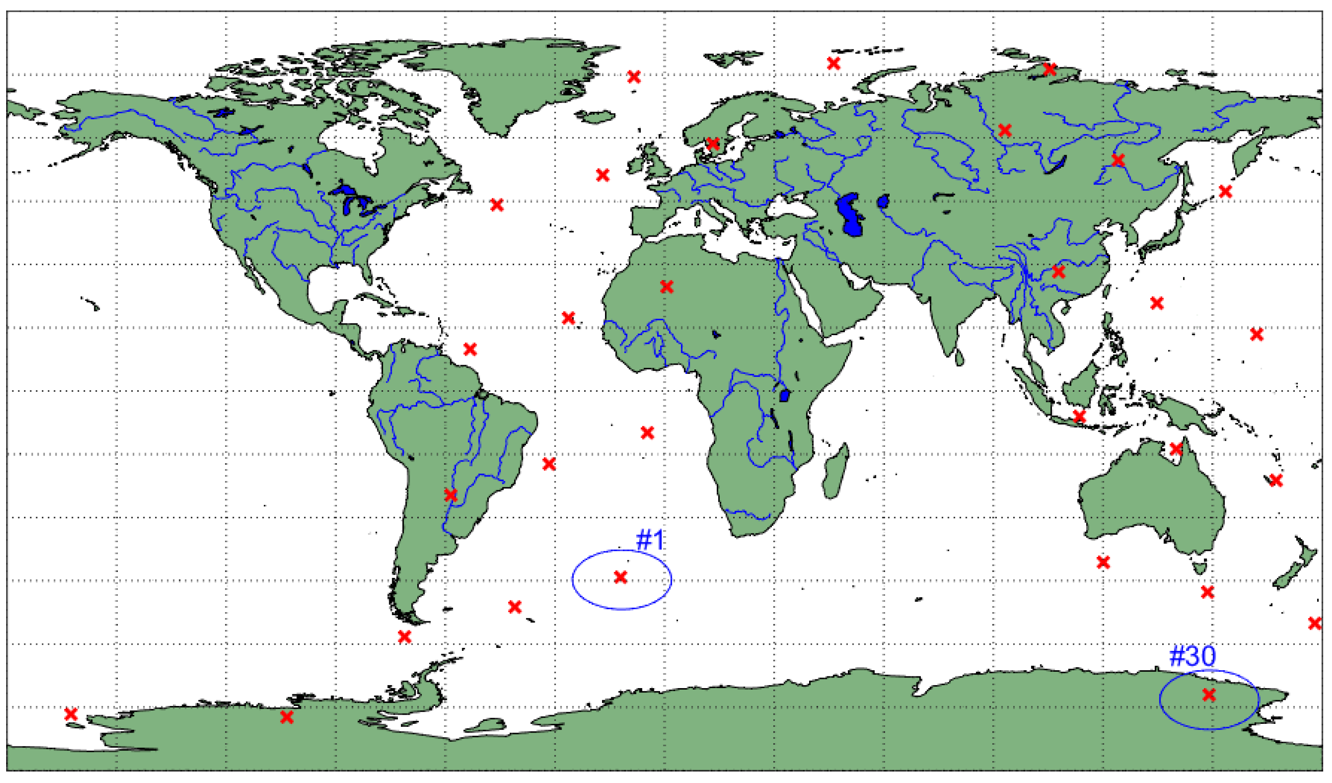
Figure 29.
In-orbit short-term monitoring of the Ku-band PTR main characteristics in blue: (a) IPD; (b) Total Power; (c) WML; (d) Sidelobes Peak Power Dissymmetry (bottom right panel). The SSPA House-Keeping temperature is represented in grey in the secondary y-axis.
Figure 29.
In-orbit short-term monitoring of the Ku-band PTR main characteristics in blue: (a) IPD; (b) Total Power; (c) WML; (d) Sidelobes Peak Power Dissymmetry (bottom right panel). The SSPA House-Keeping temperature is represented in grey in the secondary y-axis.
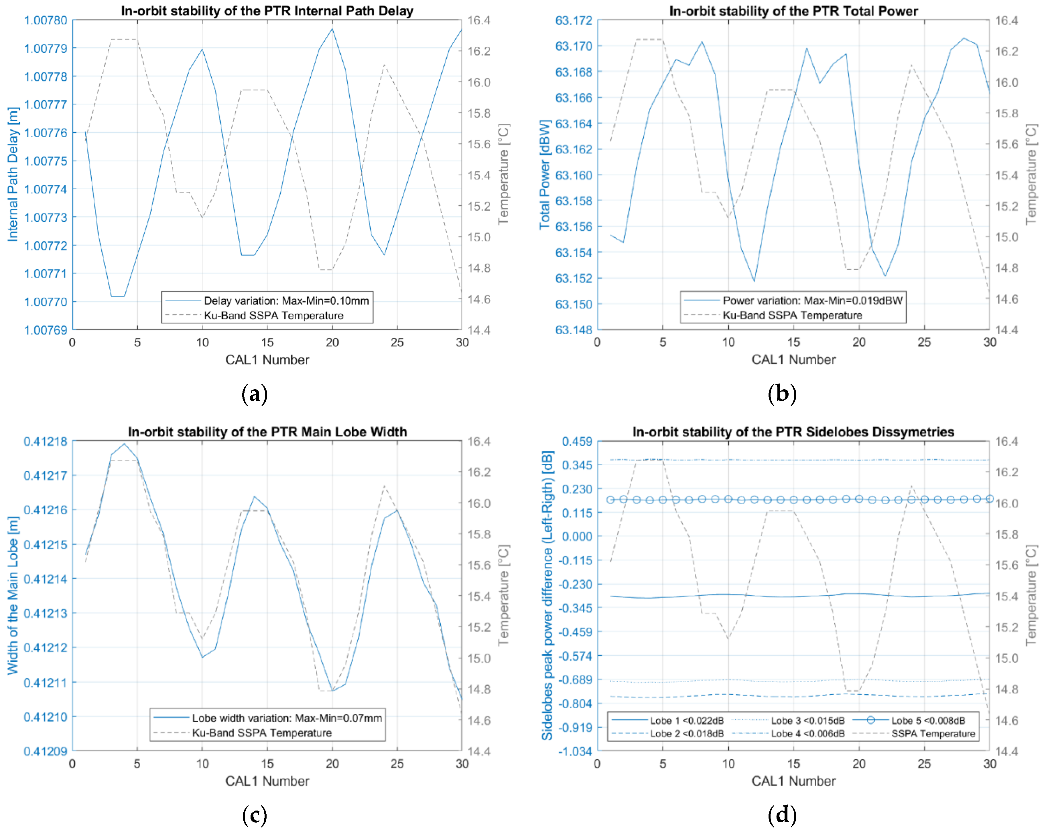
Figure 30.
Oversampled Low Pass Filter characteristics for typical ocean AGC codes, focusing on the 104 useful gates.
Figure 30.
Oversampled Low Pass Filter characteristics for typical ocean AGC codes, focusing on the 104 useful gates.
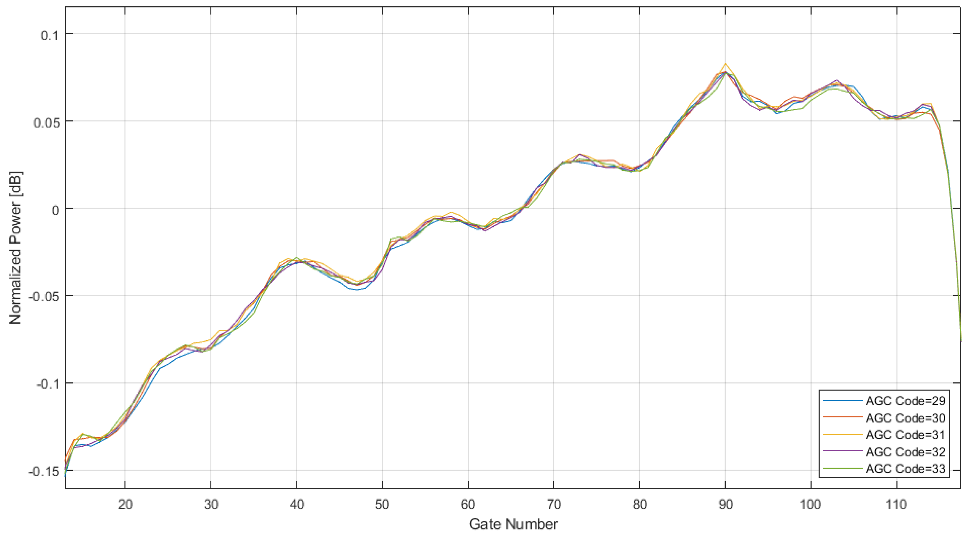

Table 1.
POSEIDON-3C operating modes, as described in Sections 2.3.1 to 2.3.3.
| Mode | Description |
|---|---|
| M1 | Autonomous acquisition and tracking |
| M2 | DIODE acquisition/autonomous tracking |
| M3 | DIODE + DEM |
| M4 | DIODE + DEM with auto transition |
| M4bis | DIODE + DEM with auto transition and direct transition from open loop to closed loop enabled |
Table 2.
Scheduling of POSEIDON-3C tracking mode changes.
| Modification date | Implemented tracking mode | |
|---|---|---|
| 16/01/2023 | M1 | Autonomous acquisition and tracking |
| 06/02/2023 | M2 | DIODE acquisition/autonomous tracking |
| 13/02/2023 | M3 | DIODE + DEM |
| 20/02/2023 | M4 | DIODE + DEM with auto transition |
| 20/03/2023 | M4bis | DIODE + DEM with auto transition and direct transition from OL to CL |
| 21/07/2023 | M1 | Autonomous acquisition and tracking |
| 09/10/2023 | M4bis | DIODE + DEM with auto transition and direct transition from OL to CL |
Table 3.
This is a table. Tables should be placed in the main text near to the first time they are cited.
Table 3.
This is a table. Tables should be placed in the main text near to the first time they are cited.
| Tracking mode | % of tracking | % of data loss |
|---|---|---|
| M1 | 99.9602 | 0.0398 |
| M4bis | 99.9994 | 0.0006 |
Table 4.
Percentage of tracking data for SWOT nadir, for mode M1 computed over cycle 1 (between 21/07/2023 11/08/2023) and for mode M4bis computed over cycle 6 (between 02/11/2023 and 23/11/2023).
Table 4.
Percentage of tracking data for SWOT nadir, for mode M1 computed over cycle 1 (between 21/07/2023 11/08/2023) and for mode M4bis computed over cycle 6 (between 02/11/2023 and 23/11/2023).
| Tracking mode | % of tracking | % of data loss |
|---|---|---|
| M1 | 98.453 | 1.547 |
| M4bis | 99.9926 | 0.0074 |
Table 5.
Number and associated percentage of saturated waveforms for different surfaces, computed over cycle 6 of SWOT compared to JASON-3 (J3).
Table 5.
Number and associated percentage of saturated waveforms for different surfaces, computed over cycle 6 of SWOT compared to JASON-3 (J3).
| Surface type | Nb SWOT | % SWOT | Nb J3 | % J3 |
|---|---|---|---|---|
| Open ocean: |lat|<55° + dist > 50 km | 18 | 0.0001% | 18 | 0.0001% |
| Land: |dist < 0 km | 155211 | 1.5% | 328304 | 3.8% |
| Sea-Ice: |lat|>55° + dist > 50 km | 159314 | 2.8% | 101721 | 1.7% |
| Coastal areas: 0km≥ dist ≥ 50 km | 41187 | 1.8% | 20243 | 1.1% |
| Total | 355730 | 1.1% | 450286 | 1.4% |
Disclaimer/Publisher’s Note: The statements, opinions and data contained in all publications are solely those of the individual author(s) and contributor(s) and not of MDPI and/or the editor(s). MDPI and/or the editor(s) disclaim responsibility for any injury to people or property resulting from any ideas, methods, instructions or products referred to in the content. |
© 2024 by the authors. Licensee MDPI, Basel, Switzerland. This article is an open access article distributed under the terms and conditions of the Creative Commons Attribution (CC BY) license (https://creativecommons.org/licenses/by/4.0/).
Copyright: This open access article is published under a Creative Commons CC BY 4.0 license, which permit the free download, distribution, and reuse, provided that the author and preprint are cited in any reuse.


