
Submitted:
28 October 2023
Posted:
30 October 2023
You are already at the latest version
Abstract
We present multi-sensor measurements from satellites, unmanned aerial vehicle, marine radar, thermal profilers and repeated conductivity-temperature-depth casts made in the Kara Gates strait connecting the Barents and the Kara Seas during spring tide in August 2021. Analysis of the field data during an 18-hour period from four stations evidence that a complex sill in the Kara Gates is the site of regular production of intense large-amplitude nonlinear internal waves. Satellite data show a presence of a relatively warm northeastward surface current from the Barents Sea toward the Kara Sea attaining 0.8-0.9 m/s. Triangle-shaped measurements of three thermal profilers revealed pronounced vertical thermocline oscillations up to 40 m associated with propagation of short-period nonlinear internal waves of depression generated by stratified flow passing a system of shallow sills in the strait. The most intense waves were recorded during the ebb tide slackening and reversal when the background flow was predominantly supercritical. Observed internal waves had wavelength of ~100 m and travelled northeastward with phase speeds of 0.8-0.9 m/s. The total internal wave energy per unit crest length for the largest waves was estimated to be equal to 1.0-1.8 MJ/m.
Keywords:
nonlinear internal waves
; large-amplitude waves
; tidal currents
; spring tide
; tidetopography interactions
; thermal profilers
; remote sensing
; UAV
; Kara Gates
; Arctic Ocean
1. Introduction
Nonlinear internal waves (NLIWs) are known to have a significant impact on the transport of energy, momentum, sediments, plankton and contaminants in the deep and coastal oceans [1,2,3,4,5]. Recent studies have clearly demonstrated the intensification of vertical mixing and anomalously high levels of turbulent energy dissipation and vertical heat fluxes due to the generation, propagation, and subsequent breaking of short-period NLIWs on the Arctic shelf and continental slope [6,7,8,9]. In recent years, more information has been appearing about new areas of large-amplitude NLIW generation in the Arctic [10,11,12,13,14].
The Kara Gates (KG) is apparently one of such regions [15,16,17]. The strait connects the Barents Sea with the Kara Sea. The region is known for its intense dynamics [18]. The transport of sea water in the strait is about 0.3-0.6 Sv [19]. The average flow velocity is in the range of 0.06-0.26 m/s, and the maximum velocity can be as high as 0.5 m/s [20]. Moreover, the KG is among areas with the most intense marine traffic in the Arctic Ocean. The Northern Sea Route, which is the main transpolar transport route connecting the Pacific and Atlantic Oceans, passes through the KG [21,22]. The ongoing active industrial development of the Russian Arctic, especially in the Kara Sea provides ~2500 ship tracks passing through KG annually [23]. Therefore, the increasing vessel traffic in the KG and oil drilling activities nearby make it essential to study local oceanographic processes that might eventually influence them.
The KG area is known for a very complex bottom topography having a complex sill with many crests unevenly distributed along and across the strait [18]. Interaction of strong tidal currents, dominated by M2 tide, with undulating topography leads to generation of intense internal tides here [15,18,24,25]. Numerous studies have also reported surface signatures of short-period NLIWs regularly registered here in satellite synthetic aperture radar (SAR) images [16,17,18,26], confirming that strong conversion of barotropic tidal energy into IWs and high levels of tidal energy dissipation occur in the region [27].
Since 1997, the study of IWs in the KG has been carried out using moorings and towed conductivity-temperature-depth (CTD) profilers recording in scanning mode [15,18,20], which made it possible to determine main characteristics of IWs and their relationship with background currents. The results of numerical modeling showed the existence of internal tides with amplitudes of 10-16 m in the strait at the Barents Sea side [25] and formation of a strong hydraulic jump with height >50 m at the Kara Sea side [18]. In these numerical experiments, the generation of short-period NLIW trains was reproduced only qualitatively. A more detailed analysis of generation and evolution of NLIWs in the strait was performed later using a two-dimensional non-hydrostatic MITgcm model that revealed the main kinematic characteristics of NLIWs and some peculiarities of their propagation at both sides of the strait [28].
Despite existing reliable information about the regular formation of NLIW trains in the KG during the interaction of tidal currents with rough bottom topography, so far, no special experiments to study their vertical structure, spatial and kinematic properties have been carried out. It is noteworthy that the strait is characterized by an extremely heterogeneous topography with many underwater ridges and channels [18], which leads to a very complex pattern of the generation and propagation of NLIW packets both along and across the strait [16].
The goal of this paper is to present new results of multi-sensor remote sensing and in situ measurements of NLIWs in the KG in August 2021 during the 58th cruise of the R/V Akademik Ioffe, documenting, for the first time, the formation and propagation of large-amplitude NLIWs in this Arctic region.
2. Materials and Methods
The KG is a 30 km long and 56 km wide strait between the southern end of the Novaya Zemlya and the northern tip of Vaygach Island connecting the Barents Sea in the west and the Kara Sea in the east (Figure 1). The bottom topography of the strait is characterized by a complex sill with several crests and troughs oriented both along (Figure 1b) and across the strait (see Figures 4, 6 in [18]).
Measurements were collected in the Kara Gates between 07:00 UTC on 12 August and 02:00 UTC on 13 August 2021. Field works were performed at latitudes 70°-71° N, which is close to the critical latitude for the lunar semidiurnal tide M2 [29,30,31]. Thus, internal tidal waves of main energetic peak at frequency M2 are forced and must dissipate locally, evolving into packets of short-period NLIWs, which can freely propagate and further transport tidal energy at high latitudes [7,32].
During the expedition, measurements included those by distributed temperature sensors (thermal profilers), frequent CTD casts, observations from an unmanned aerial vehicle (UAV), and quasi-operational analysis of satellite data. Unfortunately, the ship-mounted acoustic Doppler current profiler system was out of service, hence, a standard information on ocean current properties was not available.
Satellite information included optical, infrared and SAR data of medium and high resolution (Sentinel-1, -2, -3, MODIS Aqua/Terra, and Landsat-8). This information was downloaded and processed in near-real time by the Remote Sensing Department of MHI RAS and transmitted to the vessel for planning the measurement sites and assessing the background NLIW field in the strait.
On 12 August 2021, five stations were occupied in the strait, the position of which is shown in Figure 1a with red (start) and green (end) dots and summarized in Table 1. To determine the oceanographic background and estimate the depth of the thermocline, the vertical CTD profiles were performed at the beginning of each station using a Sea-Bird Electronics 19 plus instrument. From these data, the buoyancy frequency was computed as , where 9.8 m/s2 is the gravity acceleration, is the mean water density, and is the vertical density profile. Rapid CTD casts were performed using an autonomous AML BaseX profiler.
In order to record surface manifestations of NLIWs and correct the position of the vessel, photo and video recording was made using a DJI Mavic 2 Pro UAV from heights of 100 to 500 m at all stations where visibility conditions were favorable. We also used the records of marine navigational X-band radar JMA-9122-6XA at one station. The radar was primarily operated to study the properties of wind waves, but it was also useful to detect surface signatures of NLIWs [33]. The radar was located at an altitude of 25 m above sea level and carried out measurements with a rotation frequency of 24 rpm emitting a backscatter signal with a frequency of 9.41 GHz at a wavelength of 3.18 cm with a pulse length of 0.07 μs. The SeaVision system was used to record the radar data.
The key instrument for measuring NLIW parameters was a thermal profiler (TP) TPArctic developed at the MHI RAS with a measuring cable length of 48 m (32 continuous measuring sections each 1.5 m long), a 100 m power/communication cable, and two pressure sensors in the lower and upper sections of the line [34]. It has a digital temperature resolution of 0.0007 °C, a precision in measuring temperature over 1.5 m intervals of 0.1 °C and a sampling rate of 0.5 Hz. The main advantage of this device is its direct connection to a portable computer that provides controlled visualization of vertical profile of seawater temperature enabling to capture NLIW propagation in real-time telemetric mode. In addition, the length of the power/communication cable provides opportunity to vary depth of the instrument by means of casting, depending on the depth of the thermocline. Depth reference in this case was provided using the readings of pressure sensors.
To understand propagation direction of NLIWs, measurements with thermal sensors are often made from three spatially spaced positions in the form of a triangle (e.g., [12,35,36]). At one station (#3915), two more discrete TPs with 10 and 11 Starmon Mini StarOddi autonomous temperature sensors (with an accuracy of ±0.025 °C and sampling rate of 1 s) located at a distance of 2 m from each other in the vertical with pressure sensors DST centi TD StarOddi at the upper and lower depths of the TPs were used. Pressure sensors were used for linear correction of the TPs’ deviation from the vertical position. The total length of these TPs was more than 30 m, the measuring parts were about 20 and 22 m, respectively. Similar sensors were used to measure NLIW properties in other seas [37,38]. Onboard the ship, the TPArctic was located on the port (left) side in the center of the ship, while the discrete TPs were located on the starboard (right) side of the ship (at vessel stern and vessel bow) at a distance of 51 m between them, and from 20 m to 40 m from the TPArctic. Measurements with the TPs were carried out during a free drift of the vessel.
Information about tidal dynamics was derived from the Arctic Ocean Inverse Tide Model on a 5-kilometer grid (hereinafter, Arc5km2018) [39]. The information about the total water depth during the measurements was obtained from ELAC LAZ4700 echosounder. Since not all the bathymetry data were digitally recorded, we also used records from the navigational software OpenCPN. Wind measurements at 22 m height were made using AIRMAR WeatherStation 220 WX with temporal resolution of 1 s.
3. Results
3.1. Background Conditions in the Kara Gates
During the field works in the KG wind conditions were characterized by low to moderate winds with mean velocity of about 5 m/s during the first three stations, rising gradually to about 7 m/s toward the end of observations (Figure 2).
In the KG, the main current is directed from the Barents Sea towards the Kara Sea. Usually, it is located along the northwestern coast of Vaygach Island and may cover about 2/3 of the strait width [40], as seen in a high-resolution (~100 m) sea surface temperature (SST) map of 14 September 2016 (Figure 3a) produced from Landsat-8 data using a two-channel SST algorithm [41]. Landsat-8 perfectly resolves a surface circulation in the strait and clearly depicts a relatively warm northeastward current that typically attains 0.1-0.2 m/s peaking at 0.5 m/s [19]. MODIS Aqua SST map acquired on 9 August 2021, i.e., three days prior to measurements, shows a very similar surface pattern at 1 km resolution with the relatively warm (9-11° C) Barents Sea water covering the southeastern half of the strait (Figure 3b).
The closest to the measurement period and almost cloud-free day on 9 August 2021 provided large set of satellite data, including a number of Sentinel-3 A/B Sea and Land Surface Temperature Radiometer (SLSTR) images. A series of consequent SLSTR Level-1B thermal IR brightness temperature images at 1 km resolution was used to reconstruct the surface velocity field in the study region by applying a 4-Dvar algorithm [42]. The time gap between sequential images acquired at 16:05 and 17:46 GMT was 1 h 41 min. Figure 3c shows the resulting surface velocity vectors plotted over the absolute value of surface current velocity (shown in color). In the strait, velocity vectors were predominantly directed north and northeast. The maximal current speed of 0.8-0.9 m/s was observed in the central and northeastern parts of the strait. In the central and eastern KG, the current direction gradually turned eastward in agreement with the surface thermal expressions demonstrated in Figure 3a,b. The measured maximal surface current velocities were almost twice higher than those reported earlier [19,20], however, the analysis of the ship drift velocity presented below confirmed them.
Tidal Conditions
When studying internal waves, it is important to know the phases of the moon. In our case, the new moon was on 10 August 2021, and 12 August 2021 was the period of the growing moon. Thus, the measurements were carried out during the spring tide, which is characterized by the maximal tidal current velocities along the strait [18]. This is well illustrated in Figure 4a showing tidal variations of sea level during a two-week period on 5-19 August 2021 from Arc5km2018 pointing out the maximum amplitudes of tidal range on 11-13 August 2021.
We used Arc5km2018 model to predict the tidal currents over the period from 12 to 13 August 2021 (48 hours) using four semidiurnal constituents M2, S2, N2, K2 and four diurnal constituents K1, O1, P1, Q1. Figure 4b shows the maximum tidal current speed (in color) and the M2 ellipses in the KG. Three main areas of amplification of tidal currents in the strait can be distinguished: (a) the northwestern part of the strait near the Kusova Land and the Loginov Islands (see Figure 1a for geographic notations); (b) the eastern part of the strait along the Vaygach coast; (c) the southern part of the strait. In the areas (a) and (b) the maximal tidal current velocities expected from the Arc5km2018 model are 0.5‒0.6 m/s. In area (c), the speed of the tidal currents is 0.35‒0.45 m/s. The semidiurnal constituent M2 makes the main contribution to the total tidal current. The M2 tidal ellipses are relatively narrow and are aligned along the strait axis, averaging at 0.1-0.15 m/s. Only along the Vaygach coast (areas (b) and (c) the tidal ellipses of the M2 tide are broader and the current speed is up to 0.3-0.4 m/s.
A very complex bottom topography in the KG and pronounced tidal currents superposed on the mean currents from the Barents to the Kara Seas may cause very high horizontal velocities in the strait of the order of 1 m/s, creating favorable forcing conditions for the generation of large-amplitude NLIWs here.
Surface Signatures of NLIWs in Satellite Data
Satellite data covering the study region were operationally communicated to the expedition team for planning the locations of stations. Figure 5a shows an almost cloud-free Sentinel-2A true color image acquired over the study site on 8 August 2021, i.e., four days prior to field observations. As in situ measurements by thermal profilers were done in free drift, Figure 5 shows start and end points of stations by red and green circles, respectively.
Figure 5b shows an enlarged fragment of Sentinel-2A image with well-seen surface signatures of NLIW trains, most of which in this case were directed south and southwest. However, satellite images of other dates also showed systems of NLIWs travelling northeastward. The locations of stations were selected so that they would begin south of underwater hills and end up after crossing them while the ship freely drifted northeast.
On 11-13 August 2021, the KG region was densely covered by clouds that hindered usage of satellite optical data. In turn, Sentinel-1A/B made two SAR snapshots of the study region on 12 August at 02:43 GMT, i.e., about four hours prior to the ship arrival to the first station, and on 13 August at 02:36 UTC, i.e., just after the completion of the last station (Figure 6). However, due to low winds at the time of image acquisitions, they showed only dark elongated slicks mimicking the patterns of surface circulation (Figure 3c).
3.2. Vertical Thermohaline Measurements at Stations
As distinct thermocline oscillations presumably associated with the NLIW activity were observed only at four stations 3909-3915, below we describe the data only from these stations.
Station #3909
The first station (station #3909) was located in the western part of the KG southwest of one of the sill crests peaking at about 40 m depth (Figure 1b), behind which the formation of NLIW packets was regularly observed earlier [18]. An average water depth during the station was about 170 m (Figure 7).
At this station measurements were carried out only by the TPArctic from 08:25 to 09:28 UTC on 12 August 2021. The beginning of the station coincided with the low water and the beginning of flood (Figure 4a). According to Arc5km2018, an NNE tidal current of 0.08 m/s was present in the beginning of station, gradually rotating clockwise and decreasing to 0.06 m/s (Figure 7).
The vertical CTD cast made prior to thermal profiling revealed stable stratification and thermocline located at the depths of 25-40 m (Figure 7a). The first peak of up to 13 cph was observed at a depth of 18 m. However, the major peak was observed at a depth of about 30-35 m. Pronounced fluctuations of isotherms with heights from a few meters to 15 m and periods from 2 min to 8 min were observed (Figure 7b). Most of the record contained relatively weak oscillations not exceeding 5-6 m. However, starting from the 44th minute, i.e., closer to the sill crest located northeast, two pronounced and steep displacements of 4°C and 6°C isotherms were seen at 25–45 m depths. The first wave was rather steep, 13–15 m high with a period of 7 min. The second one was about 10 m high and had a front slope much steeper compared to the rear one.
Station #3911
The next station 3911 was planned for the vessel to drift over another sill, the shallowest along the ship route, rising upward from 150-170 m depth up to 35 m depth (Figure 1b). Field works began at 10:59 UTC and lasted for about 2 hours. The measurements were carried out during the flood tide characterized by weak currents (Figure 4a).
The vertical buoyancy profile shows two peaks at 10 m and 33 m depths (Figure 8a). The most intense fluctuations of isotherms were observed between 10 m and 40 m depths (Figure 8b). In the beginning, 5-11 m high oscillations of isotherms at a depth of 25–40 m were seen at a frequency of about 11-12 cph (Figure 8b). After 20 minutes of the free drift northward, the ship passed the sill crest. The profiler first recorded a sharp vertical rise of isotherms up to 8-15 m depth followed by a 30 m high hydraulic jump down to 43 m of the 4°C isotherm with a period of 34 minutes (Figure 8b). The next fluctuation of the 4°C isotherm at the 70th minute had almost the same period (about 30 min), but a lower height (about 20 m). Another pronounced and steep oscillation of isotherms with a height of about 20 m and a period of about 10 min was also recorded at minute 105 (Figure 8d).
At this station UAV survey was made prior to TP measurements to check whether surface signatures of NLIWs were present nearby. As a result, very characteristic sea surface manifestations of NLIWs in the form of elongated narrow slicks, usually observed under low winds [43], were detected several hundred meters northward from the ship (Figure 9). The curvature of the slick bands suggested that the waves were oriented northeastward.
During this station, the marine radar was in active mode helping to detect surface signatures of NLIWs present in thermal profiling data. The first 30-m high oscillation (centered at 37th minute in the TP record) has a clear radar manifestation as a curved, about 0.2 km wide and 2-3 km long band of alternating suppressed (from the SW side) and enhanced (from the NE side) radar echo (Figure 9a,b). This feature is similar to standard IW manifestations usually seen in spaceborne SAR data [9,18,44], suggesting that the NLIW propagation direction is toward the northeast.
At 11:16 UTC the IW signature was about 800 m northeast of the ship (Figure 9a), while between 11:31 UTC and 11:35 UTC the ship passed it away (Figure 9b). The mean ship drift velocity was about 0.8-0.9 m/s, suggesting that the observed hydraulic jump and its surface manifestation were rather stationary during this period.
Another pronounced radar manifestation was depicted at 12:37 UTC (Figure 9c). It is characterized by a smaller horizontal extent. The propagation direction of this feature is toward NE (azimuth ~40°). The passage of this feature through the vessel location corresponds well to the deepening of the isotherms centered at 108th minute of the TP record (Figure 8b). The average propagation velocity of this structure relative to the vessel was ~0.55 m/s. The average ship drift velocity during the interval of 90-105 minutes of the TP record was ~0.6 m/s. From the latter, it follows that the surface manifestation spread in the NE direction at a very low speed of ~0.05 m/s.
Station #3913
Station 3913 was located in the very center of the strait over a smaller sill crest peaking at 60 m surrounded by water depths of 100-120 m. The TPArctic measurements began at 16:18 UTC and lasted for about 80 minutes during the ebb tide. According to Arc5km2018, the northward tidal current reached 0.12 m/s at the beginning of station and raised to 0.19 m/s at the end of measurements (Figure 11).
The vertical profile of buoyancy frequency shows a clear peak in the thermocline layer at 26 m depth, amounting to 20 cph (Figure 11a). At the beginning of the record one can see several oscillations of 10-15 cph with a height of about 5–8 m (Figure 11b). More pronounced fluctuations of isotherms were seen later, after passing the sill crest on the 55th minute of the record. At this moment, rapid CTD casts down to 60 m depth with a period of about 2-4 minutes were made simultaneously with the thermal profiling. The recorded movement of isopycnals is shown in Figure 11b in green. The oscillations of isopycnals and isotherms coincide in shape and height, but have a phase shift of several minutes since the measurements were made at a distance of 35 m from each other. The maximum heights of oscillations reached 12 m at this station. This result emphasizes that the use of thermal profiling in the strait is quite justified, since the vertical water stratification significantly depends on temperature in this Arctic region.
Station #3915
Station 3915 was made at the end of the ebb tide (Figure 4a) over the deeper region (~ 140 m depth) at some distance from any pronounced bottom topography features (Figure 1b). The previous work showed a formation of a strong hydraulic jump over this part of the strait by the northeastward current over a system of sills [18].
The atmospheric conditions were characterized by 4-7 m/s winds of varying direction and strong fog that hindered UAV measurements. Unfortunately, the recording of the shipborne radar was switched off during the station. The thermal profiling began at 20:01 UTC and lasted for about 70 minutes. Measurements at this station gave the most interesting results in terms of the recorded NLIW amplitudes.
At this station the buoyancy frequency was characterized by a main peak of 21 cph at 18 m depth (Figure 12a). Vertical profiles of temperature and salinity showed a well pronounced two-layer structure with a relatively warm (~8° C) and less saline (33.7 PSU) 15-20 m thick upper layer followed by about 5-m thick pycnocline and much thicker cold (1-3° C) and more saline (~34.2 PSU) bottom layer.
The beginning of the record was characterized by rather calm conditions with only a single 7-8 m high oscillation of nearly all isotherms centered at the 7th minute of the record (Figure 12b). Yet, the most interesting features started after the 25th minute of the record. A strong and steep, nearly 30 m high depression of isotherms centered at 32nd minute with a period of 15 minutes was followed by the more intense 36-40 m high depression centered approximately at the 53rd minute with a period of 27 minutes. This second wave had a steeper rear face compared to its front. Normalized wave amplitude of both waves, i.e., the ratio of wave amplitude to the mean upper-layer depth (~20 m), was about 1.5-2. Note also a relatively flat trough of the second wave that is often observed when the wave amplitude (~40 m) occupies a significant part (~30%) of the total water depth [45,46,47]. This is a characteristic feature, also predicted by weakly nonlinear theory, when an increase in soliton amplitude is accompanied by soliton profile change from a bell-shape to a more rectangular one [48].
These two isothermal depressions, associated with the NLIW propagation, were also well seen in the movement of pycnocline recorded by rapid CTD casts (green lines in Figure 12b). The overall shapes and heights of isothermal and isopycnal depressions were similar, and had a characteristic time delay of about 2-3 minutes as those at the previous station. During the NLIW passing, measurements of the three TPs and rapid CTD casts were made simultaneously. This allowed us to estimate the propagation speed and direction of the NLIWs from characteristic time delays of their appearance in the records of different instruments (Figure 13a).
During the measurements, the ship headed southeast while drifting northeast (azimuth of 52°) with a mean speed of 0.94 m/s (Figure 13b,c). In fact, it was overtaking the wave train moving nearly in the same direction. However, as the ship moved faster than internal waves, they appeared as approaching the ship from the NNE and moving SSW at 0.1 m/s (see direction of brown arrow in Figure 13b). The summation of the ship drift vector and the NLIW propagation vector relative to the ship shows that the true propagation speed and direction of the NLIW train was 0.86 m/s to the northeast (azimuth of 56°). Based on the information about the mean period of the NLIWs, minute, and the NLIW speed relative to the vessel, their mean wavelength m, i.e., nearly equal to the water depth.
The phase speed of NLIWs can be also estimated theoretically based on available oceanographic information. The vertical stratification profile taken at this station (Figure 12a) clearly exhibits a two-layer structure allowing to apply an interfacial two-layer model for the assessment of the NLIW phase speed [9,46,49,50].
In our case, we deal with large-amplitude NLIWs for which a fully nonlinear theory should be applied [47,51]. However, several authors showed that a weakly nonlinear Korteweg–de Vries (KdV) model or its extended version (eKdV) are also valid for the moderate and large-amplitude NLIWs [52,53]. The eKdV model, including a cubic nonlinearity term, is even more applicable for such waves, provided the difference between the upper and lower layer is not large and the wave amplitude doesn’t exceed an upper bound close to half-difference between thicknesses of the layers [53,54]. As will be shown below, the latter is about 50 m and the observed 40 m high NLIWs don’t exceed it. Again, the observed broadening of the wave crest with an increase of wave amplitude (Figure 12b) is something that is well caught and predicted by the eKdV [47,55]. Owing to simple use and their wide applicability [46,47,56,57,58,59,60], below we use these models to assess the NLIW phase speed from observations.
Following [61], at first, we have to choose a suitable analytical solitary solution that depends on specific scale parameters, namely, - the thicknesses of the upper layer, - the full depth, - the half-width of the soliton, - the amplitude of NLIWs, and their ratios , , , . The half-width of the soliton is defined as , where and are the coefficients of quadratic nonlinearity and dispersion of the KdV equation [62] defined as:
where is the linear IW phase speed defined below using either Eq. (3) or Eq. (5), is the thickness of the bottom layer.
In our case, m, m, 140 m, 50 m, 30-40 m, 0.42 m/s, yielding 2.5, 0.14, 0.4, 4-5. This result lies somewhere in between the finite depth [, , O(1), O(1)] [63] and the shallow water [, O(1), O(1)] [64] theories. We, therefore, will apply both theories to estimate the nonlinear phase speed .
In two-layer model, the phase speed of linear internal waves of the lowest internal mode can be defined as [65]:
where is the density difference between the waters below and above the pycnocline, is the mean water density below the pycnocline, is the gravity acceleration, is the wave number defined as , where is the characteristic wavelength of NLIWs from observations. In case of the finite depth theory, the nonlinear soliton speed can be found as [63]:
where is the wave number-like parameter satisfying the relationship , and .
In case of shallow water, the equation for the linear phase speed of the KdV model will take form [66]:
while that for the nonlinear soliton speed would be equal to:
with an additional coefficient of cubic nonlinearity, , in the eKdV model:
with defined as:
Lastly, we also use equation to derive phase speed of strongly nonlinear waves [54]:
with defined from (5).
At station 3915, the characteristic values are = 1.75 kg/m3, = 1028 kg/m3, and = 130 m. The theoretical values are presented in Table 2. Each of them has a certain range of values because of two values of amplitude (30 and 40 m) used in the calculations. In most cases, theoretical values are somewhat lower than the observed phase speed of 0.87 m/s. The best correspondence is obtained for the KdV model (eqs. 5, 6) and that for the strongly nonlinear waves (eqs. 5, 9). Notably, the inclusion of cubic nonlinearity term (0.001 m-1s-1) in the eKdV equation (Eq. 7) significantly decreases the nonlinear phase speed values compared to the KdV model (Table 2).
In our case, the total energy equals to 1.0-1.8 MJ/m for these two large-amplitude waves.
In order to examine the possible NLIW generation mechanism we should look more closely to the flow conditions characterized by Froude number, , controlling the generation and propagation of NLIWs when the stratified flow passes over undulating topography. The Froude number is defined as the ratio of the total current vector to the phase speed of long linear internal waves (). The latter is defined from the vertical profile shown in Figure 12a using Eq. 3 ( 0.42 m/s) and Eq. 5 ( 0.54 m/s).
Due to the absence of in situ current meter measurements we use ship drift velocity to approximately define . In such case, we assume that the actual ship drift is a sum of ocean current velocity and wind-induced ship drift. As a coarse estimate, we presume that the latter doesn’t exceed 2% (using analogy to Nansen–Ekman ice-drift law [67]) of the maximum wind speed of 7-8 m/s observed prior and during the station (Figure 2).
After subtraction of the wind component, the ship drift velocity vector is converted into orthogonal components with oriented cross-strait perpendicular to the NLIW direction (azimuth 146°), and oriented northeast (azimuth 56°) along the strait and the NLIW propagation direction. In such configuration, we presume that component dominates in creation of the initial pycnocline disturbance during the ebb tide that might further evolve into the train of nonlinear waves.
During station 3915, the NLIWs were recorded between the 25th and 65th minutes when the surface current started to slack and changed direction from northeast to east, presumably due to the ebb tide slackening and reversal, well depicted in Figure 14a and Figure 12c.
In the record, ranges from 0.1 to 1.4 m/s, being at the maximum prior to and after the passing of NLIWs (Figure 14a). During the NLIW passage, drops down first by ~0.5 m/s (from 1.2 m/s to 0.7 m/s) and later down to 0.3 m/s at the 50th minute, followed by a rapid rise to 1-1.4 m/s after the waves’ passing.
The Froude number, calculated for two values of (Table 2), is supercritical for the most of the record (Figure 14b). It passes through the critical value of several times. During the NLIW passage, it drops down to near-critical (~ 1) and subcritical (< 1) values, similarly as reported by Fer et al. [8] during the passage of 50 m high NLIWs north of Svalbard.
4. Discussion
The obtained results are solidly grounded on previous observational and numerical studies in the Kata Gates [16,17,18,25,27,28]. However, our record shows much larger internal waves than were observed or predicted before. One of such reasons could be that our measurements were made exactly during the peak spring tide when the tidal forcing was maximal.
Figure 15 shows a generalized 2-d scheme of NLIW locations over the KG topography along the ship route. The recorded NLIWs were detected both immediately over the sill crests or in close proximity to them (stations 3909-3913), as well as at some distance from them (station 3915). The wavelengths of the observed NLIWs (~100-200 m) were of the same scale as narrow sill crests passed by the ship during a free drift.
An intense along strait flow composed of the mean current from the Barents Sea superposed with pronounced barotropic tide results in strong baroclinic response and NLIW generation in the Kara Gates. Vlasenko et al. [32] show that in the vicinity of critical latitude for the M2 tide (74.5° N) two main options of baroclinic response exist depending on flow regime. In subcritical regime (<1), only weak, large wavelength and small-amplitude baroclinic tides are generated. When the flow is supercritical (>1), topography-scale short NLIWs are generated, exactly as observed in our case.
Moreover, Vlasenko et al. [32] also showed a possibility for the generation of “double waves” that is caused due to the nonlinearity and the wave energy transfer from the tidal frequency to the higher harmonics. Notably, the shape of high-amplitude NLIWs at station 3915 (Figure 12) is very similar to that predicted by numerical model (see Figure 9 in [32]).
It is also interesting to compare our results with those obtained from nonhydrostatic model by Li et al. [28]. While these authors used much more simplified topography in the strait, the overall structure of NLIWs’ generation was predicted qualitatively well. In particular, they showed that the waves generated on the Kara Sea side were weaker than those on the Barents Sea side, and disintegration of the initial pycnocline disturbances occurred at about 25-30 km from the sill. The model phase speed of the waves travelling to the Kara Sea was 0.72 m/s, somewhat less than in our observations.
However, the major difference between our observations and the model is found for the case when the latter accounted for a steady background current toward the Kara Sea, which is observed in reality. In such case, the model predicted a generation of only a weak internal bore on the Kara Sea side with a small vertical displacement and not disintegrating into the wave train, while our measurements show at least two pronounced large-amplitude waves propagating at about 0.9 m/s. We presume that this discrepancy is most probably related to the lack of the detailed topography in the model simulations. Once included, it might be practical then to clarify what particular sill crest is responsible for the generation of large-amplitude NLIWs at station 3915.
Owing to radial spreading, the intense NLIWs originating from the KG are known to propagate farther offshore to the Barents and Kara Seas [16,17,18] where they could be still enough energetic to be a concern for drilling operations at many offshore oil production sites located nearby. Moreover, one can also expect a possible impact of large-amplitude NLIWs on sediment resuspension both at the strait margins and farther offshore [4].
Our observations evidence that the NLIWs generated in the KG are among the largest ever documented in the Arctic, including those with heights of 36-50 m registered over the northern flanks of the Yermak Plateau [68,69], those of ~50 m registered north of Svalbard [8], and those of 40-50 m registered in Franz Victoria Trough [30,36] and southeast of Hopen Island [13] in the Barents Sea.
While the KG is one of major spots of depth-integrated baroclinic tidal energy dissipation (>10 W/m2) in the Barents Sea [27], it is characterized by rather moderate tidal forcing in the Arctic [70,71]. The latter suggests that similar intense large-amplitude NLIWs might be also forming in other Arctic regions with rough topography and identical flow conditions.
5. Conclusions
In this work we report the results of the experimental observations specifically targeted to resolve short-period NLIWs in the Kara Gates. Synergistic use of remote sensing observations, marine radar, three spaced-apart thermal profilers and rapid CTD casts enabled to record anomalously large NLIWs forming in the KG with amplitudes up to 40 m, i.e., about one third of the total water depth in the strait.
Analysis of high- and medium-resolution satellite optical data clearly revealed main patterns of the surface circulation in the strait, depicting a presence of a relatively warm northeastward current from the Barents Sea toward the Kara Sea attaining velocities of 0.8-0.9 m/s. Prediction of tidal currents using Arc5km2018 model showed the maximal tidal current velocities along the ship route reaching 0.20-0.25 m/s. As a result, the combination of local complex bottom topography and intense currents created favorable forcing conditions for the generation of intense NLIWs here.
Quasi-operational observations of sea surface state in the strait from satellites and UAV was an important component of the experimental work that allowed us to plan the location of stations and trace the surface signatures of NLIW in the strait.
As the vertical density distribution in the study region strongly depended on seawater temperature, shipborne measurements of three spaced-apart thermal profilers allowed us to record numerous pronounced thermocline oscillations in the water layer of 10 to 65 m depth. We associated these oscillations with propagation of NLIWs of depression generated when the stratified flow passed a system of shallow sills in the strait.
The amplitudes of the observed internal waves ranged from 4 to 40 m, revealing the existence of very intense large-amplitude NLIWs in this region. The total internal wave energy per unit crest length for the largest waves was estimated to be equal to 1.0-1.8 MJ/m. The waves were recorded both immediately after passing the shallow sills and at some distance from them. The most intense NLIWs were recorded during the ebb tide slackening and reversal when the background flow was predominantly supercritical.
Measurements of the three spaced-apart TPs enabled to assess the phase speed and propagation direction of the large-amplitude NLIWs. The waves travelled northeastward with phase speeds of about 0.9 m/s. Theoretical predictions of NLIW phase speed made within a two-layer approach showed that the shallow water KdV model and that for strongly nonlinear waves agreed best with observations.
Obviously, the current meter data were lacking in our study to precisely relate the observed thermocline oscillations to the forcing conditions. In this sense, longer fixed-point measurements covering 1-2 complete M2 tidal cycles would be needed in future to clarify the NLIW generation mechanism and periodicity within a tidal cycle. The future goal is also to study the evolution and possible impacts of NLIWs on water hydrology, turbulent mixing and biogeochemical fluxes using synergistic multi-sensor observations.
Author Contributions
Conceptualization, I.E.K.; methodology, I.E.K., K.P.S, D.I.F., P.V.G., A.V.G., E.V.P.; software, I.O.K., I.E.K., D.I.F.,A.V.G., I.P.M., E.V.P., D.M.S., V.R.Z., P.V.G.; formal analysis, I.E.K., I.O.K., E.G.M., D.I.F., E.V.P., K.P.S., I.P.M.; investigation, I.E.K., I.O.K., E.G.M.; data curation, I.E.K., I.O.K., D.I.F., I.P.M., A.A.O., N.B.S.; writing—original draft preparation, I.E.K.; writing—review and editing, all authors; visualization, I.E.K., I.O.K., I.P.M., E.E., D.M.S., E.V.P.; supervision, I.E.K., A.A.O, N.B.S.; project administration, I.E.K., A.A.O, N.B.S.; funding acquisition, I.E.K., A.A.O, N.B.S. All authors have read and agreed to the published version of the manuscript.
Funding
This work was supported by the Russian Science Foundation grant No. 21-17-00278. Expedition AI-58 was carried out as part of the “Floating University” program with the support of the Ministry of Science and Higher Education of the Russian Federation.
Data Availability Statement
Sentinel-1, -2, -3 data can be freely accessed from the Copernicus Open Access Hub at https://scihub.copernicus.eu. The cruise data could be accessed from the authors upon reasonable request.
Conflicts of Interest
The authors declare no conflict of interest. The funders had no role in the design of the study; in the collection, analyses, or interpretation of data; in the writing of the manuscript, or in the decision to publish the results.
References
- Pineda, J. Predictable upwelling and the shoreward transport of planktonic larvae by internal tidal bores. Science 1991, 253, 548–549. [Google Scholar] [CrossRef] [PubMed]
- Moum, J.N.; Farmer, D.M.; Smyth, W.D.; Armi, L.; Vagle, S. Structure and Generation of Turbulence at Interfaces Strained by Internal Solitary Waves Propagating Shoreward over the Continental Shelf. J. Phys. Ocean. 2003, 33, 2093–2112. [Google Scholar] [CrossRef]
- Moum, J.N.; Nash, J.D. Seafloor pressure measurements of nonlinear internal waves. J. Phys. Ocean. 2008, 38, 481–491. [Google Scholar] [CrossRef]
- Boegman, L.; Stastna, M. Sediment Resuspension and Transport by Internal Solitary Waves. Ann. Rev. Fluid Mech 2019, 51, 129–154. [Google Scholar] [CrossRef]
- Edge, W.C.; Jones, N.L.; Rayson, M.D.; Ivey, G.N. Calibrated suspended sediment observations beneath large amplitude non-linear internal waves. J. Geophys. Res. Ocean. 2021, 126, e2021JC017538. [Google Scholar] [CrossRef]
- Padman, L.; Dillon, T.M. Turbulent mixing near the Yermak Plateau during the coordinated Eastern Arctic Experiment. J. Geophys. Res. Ocean. 1991, 96, 4769–4782. [Google Scholar] [CrossRef]
- Rippeth, T.P.; Vlasenko, V.; Stashchuk, N.; Scannell, B.D.; Green, J.A.M.; Lincoln, B.J.; Bacon, S. Tidal conversion and mixing poleward of the critical latitude (an Arctic case study), Geophys. Res. Lett. 2017, 44, 12349–12357. [Google Scholar] [CrossRef]
- Fer I., Koenig Z., Kozlov I. E., Ostrowski M., Rippeth T. P., Padman L., Bosse A., Kolas E., Tidally forced lee waves drive turbulent mixing along the Arctic Ocean margins. Geophys. Res. Lett. 2020, 47. [CrossRef]
- Kozlov, I.E.; Atadzhanova, O.A.; Zimin, A.V. Internal solitary waves in the White Sea: hot-spots, structure, and kinematics from multi-sensor observations. Remote Sens. 2022, 14, 4948. [Google Scholar] [CrossRef]
- Kozlov, I.; Romanenkov, D.; Zimin, A.; Chapron, B. SAR observing large-scale nonlinear internal waves in the White Sea. Remote Sens. Environ. 2014, 147, 99–107. [Google Scholar] [CrossRef]
- Kozlov, I.E.; Zubkova, E.V.; Kudryavtsev, V.N. Internal solitary waves in the Laptev Sea: first results of spaceborne SAR observations. IEEE Geosci. Remote Sens. Lett. 2017, 14, 2047–2051. [Google Scholar] [CrossRef]
- Zimin, A.V.; Kozlov, I.E.; Atadzhanova, O.A.; Chapron, B. Monitoring short-period internal waves in the White Sea. Izv. Atmos. Ocean. Phys. 2016, 52, 951–960. [Google Scholar] [CrossRef]
- Marchenko, A.V.; Morozov, E.G.; Kozlov, I.E.; Frey, D.I. High-amplitude internal waves southeast of Spitsbergen. Cont. Shelf Res. 2021, 227, 104523. [Google Scholar] [CrossRef]
- Morozov, E.G.; Pisarev, S.V. Internal Waves in the Region of the Akselsundet Strait of Western Spitsbergen Island. Izv. Atmos. Ocean. Phys. 2023, 59, 432–442. [Google Scholar] [CrossRef]
- Morozov, E.G.; Paka, V.T.; Bakhanov, V.V. Strong internal tides in the Kara Gates Strait. Geophys. Res. Lett. 2008, 35, L16603. [Google Scholar] [CrossRef]
- Kozlov, I.; Kudryavtsev, V.; Zubkova, E.V.; Zimin, A.V.; Chapron, B. Characteristics of short-period internal waves in the Kara Sea. Izv. Atmos. Ocean. Phys. 2015, 51, 1073–1087. [Google Scholar] [CrossRef]
- Kozlov, I.; Kudryavtsev, V.; Zubkova, E.; Atadzhanova, O.; Zimin, A.; Romanenkov, D.; Myasoedov, A.; Chapron, B. SAR observations of internal waves in the Russian Arctic seas. In Proceedings of the 2015 IEEE International Geoscience and Remote Sensing Symposium (IGARSS), Milan, Italy, 26–31 July 2015; pp. 947–949. [Google Scholar]
- Morozov, E.G.; Kozlov, I.E.; Shchuka, S.A.; Frey, D.I. Internal tide in the Kara Gates Strait. Oceanology 2017, 57, 8–18. [Google Scholar] [CrossRef]
- Harms, I.H.; Karcher, M.J. Modeling the seasonal variability of circulation and hydrography in the Kara Sea. J. Geophys. Res. 1999, 104, 13431–13448. [Google Scholar] [CrossRef]
- Morozov, E.G.; Neiman, V.G.; Shcherbinin, A.D. Internal tide in the Kara Strait. Dokl. Earth Sci. 2003, 393, 1312–1314. [Google Scholar]
- Didenko, N.I.; Cherenkov, V.I. Economic and geopolitical aspects of developing the Northern Sea Route. IOP Conf. Ser.: Earth Environ. Sci. 2018, 180, 012012. [Google Scholar] [CrossRef]
- Boylan, B.M. Increased maritime traffic in the Arctic: Implications for governance of Arctic sea routes. Mar. Pol. 2021, 131, 104566. [Google Scholar] [CrossRef]
- Gunnarsson, B. Recent ship traffic and developing shipping trends on the Northern Sea Route—Policy implications for future arctic shipping. Mar. Pol. 2021, 124, 104369. [Google Scholar] [CrossRef]
- Morozov, E.G.; Pisarev, S.V.; Erofeeva, S.Yu. Internal waves in the Russian Arctic seas. Surface and internal waves in the Arctic Ocean / Eds. I. V. Lavrenov, E. G. Morozov. Saint-Petersburg, Gidrometeoizdat. 2002; 217–234. (In Russian) [Google Scholar]
- Kagan, B.A.; Timofeev, A.A. Modeling of the Stationary Circulation and Semidiurnal Surface and Internal Tides in the Strait of Kara Gates. Fund. Appl. Hydrophys 2015, 8, 72–79, (In Russ.). [Google Scholar]
- Kozlov, I. SAR signatures of oceanic internal waves in the Barents Sea. Proc. of the SAR Oceanogr. Workshop (SeaSAR). Frascati, Italy. 2008. [Google Scholar]
- Kagan, B.A.; Sofina, E.V. Surface and internal semidiurnal tides and tidally induced diapycnal diffusion in the Barents Sea: a numerical study. Cont. Shelf Res. 2014, 91, 158–170. [Google Scholar] [CrossRef]
- Li, Q.; Wu, H.; Yang, H.; Zhang, Z. A numerical simulation of the generation and evolution of nonlinear internal waves across the Kara Strait. Acta Ocean. Sinica 2019, 38, 1–9. [Google Scholar] [CrossRef]
- Konyaev, K.V. Internal tide at the critical latitude. Izv. Atm. Ocean. Phys. 2000, 36, 363–375. [Google Scholar]
- Morozov, E.G.; Pisarev, S.V. Internal tides at the Arctic latitudes (numerical experiments). Oceanology 2002, 42, 153–161. [Google Scholar]
- Morozov, E.G.; Paka, V.T. Internal waves in a high-latitude region. Oceanology 2010, 50, 668–674. [Google Scholar] [CrossRef]
- Vlasenko, V.; Stashchuk, N.; Hutter, K.; Sabinin, K. Nonlinear internal waves forced by tides near the critical latitude. Deep Sea Res. Part I. 2003, 50, 317–338. [Google Scholar] [CrossRef]
- Ermoshkin, A.; Molkov, A. High-Resolution Radar Sensing Sea Surface States During AMK-82 Cruise. IEEE J. Select. Topics Appl. Earth Obs. Remote Sens. 2022, 15, 2660–2666. [Google Scholar] [CrossRef]
- Gaisky, P.V.; Kozlov, I.E. Thermoprofilemeter for Measuring the Vertical Temperature Distribution in the Upper 100-Meter Layer of the Sea and its Testing in the Arctic Basin. Ecol. Saf. Coast. Shelf Zones Sea 2023, 1, 137–145. [Google Scholar]
- Sandven, S.; Johannessen, O.M. High-frequency internal wave observations in the marginal ice zone. J. Geophys. Res. 1987, 92(C7), 6911–6920. [Google Scholar] [CrossRef]
- Pisarev, S.V. Low-frequency internal waves near the shelf edge of the Arctic 865 basin. Oceanology 1996, 36, 771–778. [Google Scholar]
- Serebryany, A.; Khimchenko, E.; Popov, O.; Denisov, D.; Kenigsberger, G. Internal Waves Study on a Narrow Steep Shelf of the Black Sea Using the Spatial Antenna of Line Temperature Sensors. J. Mar. Sci. Eng. 2020, 8, 833. [Google Scholar] [CrossRef]
- Silvestrova, K.; Myslenkov, S.; Puzina, O.; Mizyuk, A.; Bykhalova, O. Water Structure in the Utrish Nature Reserve (Black Sea) during 2020–2021 According to Thermistor Chain Data. J. Mar. Sci. Eng. 2023, 11, 887. [Google Scholar] [CrossRef]
- Erofeeva, S.; Egbert, G. Arc5km2018: Arctic Ocean Inverse Tide Model on a 5 kilometer grid. Dataset, Arctic Data Center. 2018. [Google Scholar] [CrossRef]
- Rogozhin, V.; Osadchiev, A.; Konovalova, O.P. Structure and variability of the Pechora plume in the southeastern part of the Barents Sea. Front. Mar. Sci. 2023, 10, 1052044. [Google Scholar] [CrossRef]
- Aleskerova, A.A.; Kubryakov, A.A.; Stanichny, S.V. A two-channel method for retrieval of the Black Sea surface temperature from Landsat-8 measurement. Izv. Atm. Ocean. Phys. 2017, 52, 1155–1161. [Google Scholar] [CrossRef]
- Korotaev, G.; Andreas, E.; Ledimet, F.; Herlin, I.; Stanichny, S.; Solovyev, D.; Wu, L. Retrieving ocean surface current by 4-D variational assimilation of sea surface temperature images. Remote Sens. Environ. 2008, 112, 1464–1475. [Google Scholar] [CrossRef]
- da Silva, J.C.B.; Ermakov, S.A.; Robinson, I.S.; Jeans, D.R.G.; Kijashko, S.V. Role of surface films in ERS SAR signatures of internal waves on the shelf: 1. Short-period internal waves. J. Geophys. Res. 1998, 103, 8009–8031. [Google Scholar] [CrossRef]
- Kudryavtsev, V.; Kozlov, I.; Chapron, B.; Johannessen, J.A. Quad-polarization SAR features of ocean currents. J. Geophys. Res. Ocean. 2014, 119, 6046–6065. [Google Scholar] [CrossRef]
- Duda, T.F.; Lynch, J.F.; Irish, J.D.; Beardsley, R.C.; Ramp S.R.; et al. Internal tide and nonlinear wave behavior in the continental slope in the northern South China Sea. IEEE J. Ocean. Eng. 2004, 29, 1105–1130. [CrossRef]
- Zhao, Z.; Klemas, V.; Zheng, Q.; Li, X.; Yan, X.-H. Estimating parameters of a two-layer stratified ocean from polarity conversion of internal solitary waves observed in satellite SAR images. Remote Sens. Environ. 2004, 92, 276–287. [Google Scholar] [CrossRef]
- Helfrich, K.R.; Melville, W.K. Long nonlinear internal waves. Annu. Rev. Fluid Mech. 2006, 38, 395–425. [Google Scholar] [CrossRef]
- Ostrovsky, L.A.; Stepanyants, Y.A. Internal solitons in laboratory experiments: Comparison with theoretical models. Chaos. Interdisc. J. Nonlin. Sci. 2005, 15, 03711. [Google Scholar] [CrossRef] [PubMed]
- Liu, A.K.; Chang, Y. S.; Hsu, M.-K.; Liang, N. K. Evolution of nonlinear internal waves in the East and South China Seas. J. Geophys. Res. 1998, 103, 7995–8008. [Google Scholar] [CrossRef]
- Petrusevich, V.Y.; Dmitrenko, I.A.; Kozlov, I.E.; Kirillov, S.A.; Kuzyk, Z.Z.; Komarov, A.S.; Heath, J.P.; Barber, D.G.; Ehn, J.K. Tidally-generated internal waves in Southeast Hudson Bay. Cont. Shelf Res. 2018, 167, 65–76. [Google Scholar] [CrossRef]
- Grue, J.; Jensen, A.; Rusas, P.; Sveen, J. Properties of large-amplitude internal waves. Journal of Fluid Mechanics. 1999, 380, 257–278. [Google Scholar] [CrossRef]
- Kao, T.W.; Pan, F.-S.; Renouard, D. Internal solitons on the pycnocline: generation, propagation, and shoaling and breaking over a slope. J. Fluid Mech. 1985, 59, 19. [Google Scholar] [CrossRef]
- Gerkema, T.; Zimmerman, J.T.F. An introduction to internal waves. Lecture notes, Royal NIOZ, Texel 2008. [Google Scholar]
- Ostrovsky, L.A.; Irisov, V.G. Strongly nonlinear internal solitons: Models and applications. J. Geophys. Res. Oceans. 2017, 122, 3907–3916. [Google Scholar] [CrossRef]
- Stanton, T.P.; Ostrovsky, L.A. Observations of highly nonlinear internal solitons over the continental shelf. Geophys. Res. Lett. 1998, 25, 2695–2698. [Google Scholar] [CrossRef]
- Osborne, A.R.; Burch, T. L. Internal solitons in the Andaman Sea. Science. 1980, 208, 451–460. [Google Scholar] [CrossRef] [PubMed]
- Porter, D.J.; Thompson, D.R. Continental shelf parameters inferred from SAR internal wave observations. Journal of Atmospheric and Oceanic Technology. 1999, 16, 475–487. [Google Scholar] [CrossRef]
- Zheng, Q.; Yuan, Y.; Klemas, V.; Yan, X.-H. Theoretical expression for an ocean internal soliton synthetic aperture radar image and determination of the soliton characteristic half width. J. Geophys. Res. 2001, 106(C12), 31415–31423. [Google Scholar] [CrossRef]
- Zhang, Y.; Hong, M.; Zhang, Y.; Zhang, X.; Cai, J.; Xu, T.; Guo, Z. Characteristics of Internal Solitary Waves in the Timor Sea Observed by SAR Satellite. Remote Sens. 2023, 15, 2878. [Google Scholar] [CrossRef]
- Peng, P.; Xie, J.; Du, H.; Wang, S.; Xuan, P.; Wang, G.; Wei, G.; Cai, S. Analysis of the Differences in Internal Solitary Wave Characteristics Retrieved from Synthetic Aperture Radar Images under Different Background Environments in the Northern South China Sea. Remote Sens. 2023, 15, 3624. [Google Scholar] [CrossRef]
- Zheng, Q.; Yan, X.-H.; Klemas, V. Statistical and dynamical analysis of internal waves on the continental shelf of the Middle Atlantic Bight from space shuttle photographs. J. Geophys. Res. 1993, 98(C5), 8495–8504. [Google Scholar] [CrossRef]
- Ostrovsky, L.A.; Stepanyants, Y.A. Do internal solitons exist in the ocean? Rev. Geophys. 1989, 27, 293–310. [Google Scholar] [CrossRef]
- Joseph, R.I. Solitary waves in a finite depth fluid. J. Phys. A Mark. Gen. 1977, 10, L225–L227. [Google Scholar] [CrossRef]
- Benjamin, T.B. Internal waves of finite amplitude and permanent form. J. Fluid Mech. 1966, 25, 241–270. [Google Scholar] [CrossRef]
- Phillips, O.M. The Dynamics of the Upper Ocean, 2nd ed.; Cambridge Univ. Press: Cambridge, UK, 1980; 336p. [Google Scholar]
- Grimshaw, R.; Pelinovsky, E.; Talipova, T. Solitary wave transformation in a medium with sign-variable quadratic nonlinearity and cubic nonlinearity. Physica D. 1999, 132, 40–62. [Google Scholar] [CrossRef]
- Leppäranta, M. The drift of sea ice, 2nd ed.; Springer Praxis Books; Springer-Verlag, 2011. [Google Scholar] [CrossRef]
- Czipott, P.V.; Levine, M.D.; Paulson, C.A.; Menemenlis, D.; Farmer, D.M.; Williams, R.G. Ice flexure forced by internal wave packets in the Arctic Ocean. Science 1991, 254, 832–835. [Google Scholar] [CrossRef] [PubMed]
- Padman, L.; Dillon, T. M. Turbulent mixing near the Yermak Plateau during the Coordinated Eastern Arctic Experiment. J. Geophys. Res. 1991, 96(C3), 4769–4782. [Google Scholar] [CrossRef]
- Kowalik, Z.; Proshutinsky, A.Y. “The Arctic Ocean tides” in The Polar Oceans Their Role Shaping Global Environment; Johannessen, O.M., Muench, R.D., Overland, J.E., Eds.; AGU: Washington, DC, USA, 1994; pp. 137–158. [Google Scholar]
- Padman, L.; Erofeeva, S. A barotropic inverse tidal model for the Arctic Ocean. Geophys. Res. Lett. 2004, 31, 2. [Google Scholar] [CrossRef]
Figure 1.
(a) Bathymetric map of the KG based on the GEBCO2021 data. Locations of stations are shown by red (start) and green (end) dots; (b) bottom topography along the KG from shipborne echosounder (blue) and OpenCPN navigation software (green). The inset in panel (a) demonstrates location of the study area between the Barents and the Kara Seas.
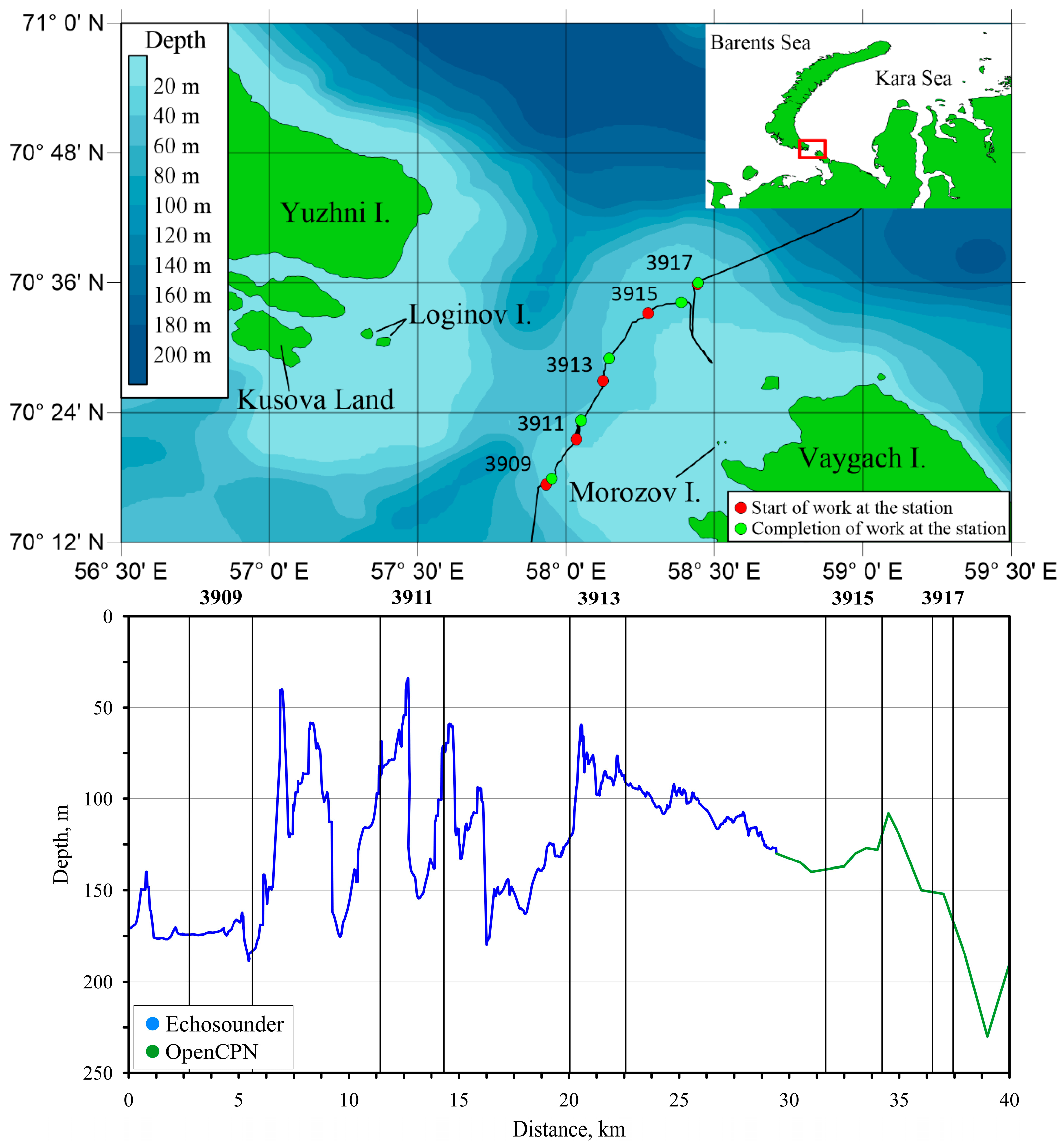
Figure 2.
Wind speed on 12-13 August 2021 recorded at the vessel at 22 m height. Grey line indicates measurements with temporal resolution of 1 minute, while blue line shows measurements averaged by 1 hour.
Figure 2.
Wind speed on 12-13 August 2021 recorded at the vessel at 22 m height. Grey line indicates measurements with temporal resolution of 1 minute, while blue line shows measurements averaged by 1 hour.
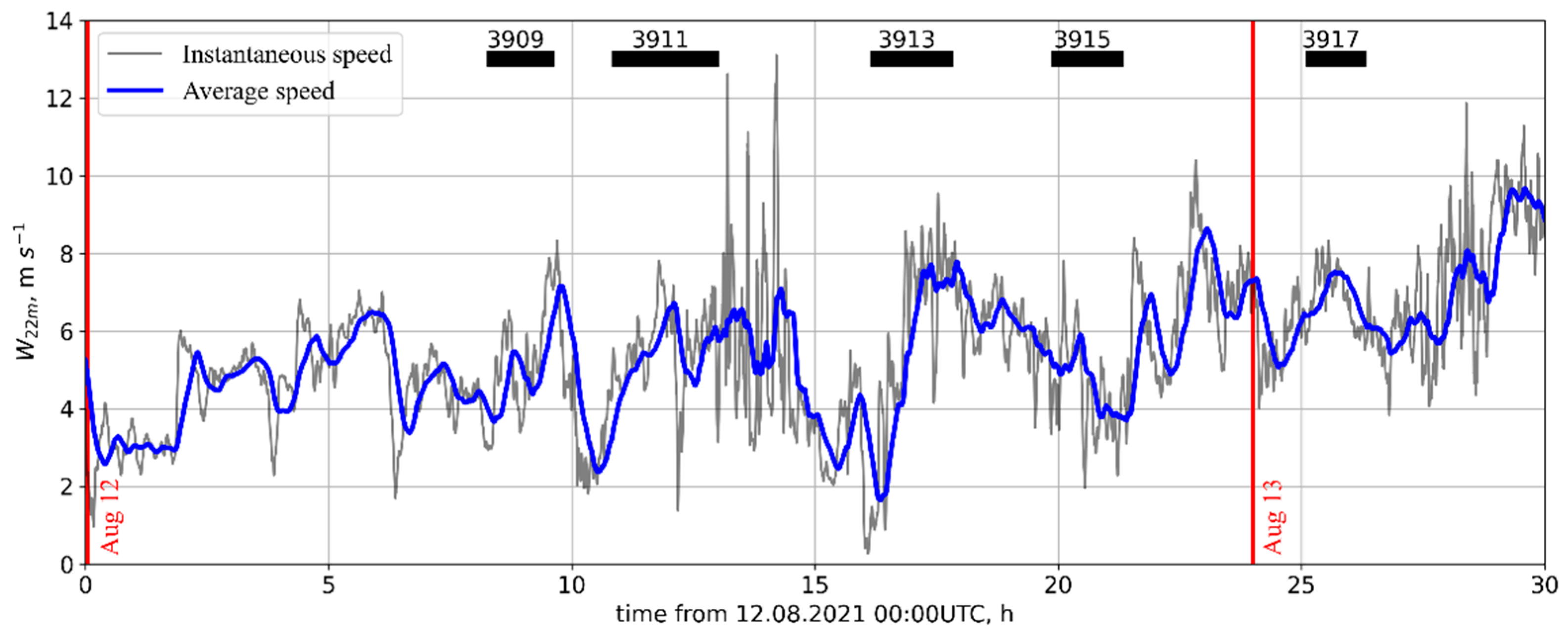
Figure 3.
Horizontal structure of sea surface temperature and currents in the KG: (a) Landsat-8 SST map of 14 September 2016 (08:00 GMT); (b) MODIS Aqua SST map of 9 August 2021 (07:55 GMT); (c) surface current vectors and magnitude derived from sequential SLSTR thermal IR images acquired on 9 August 2021 (16:05 GMT).
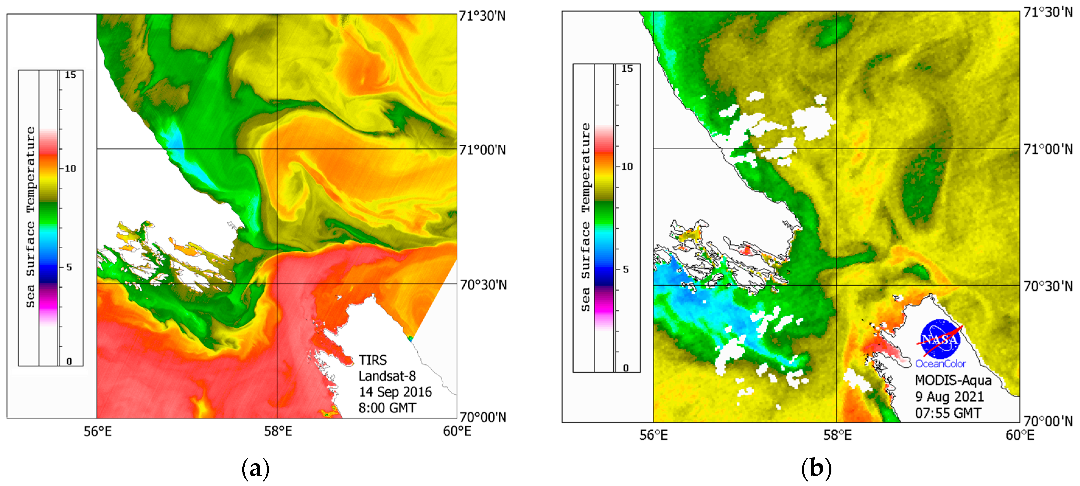
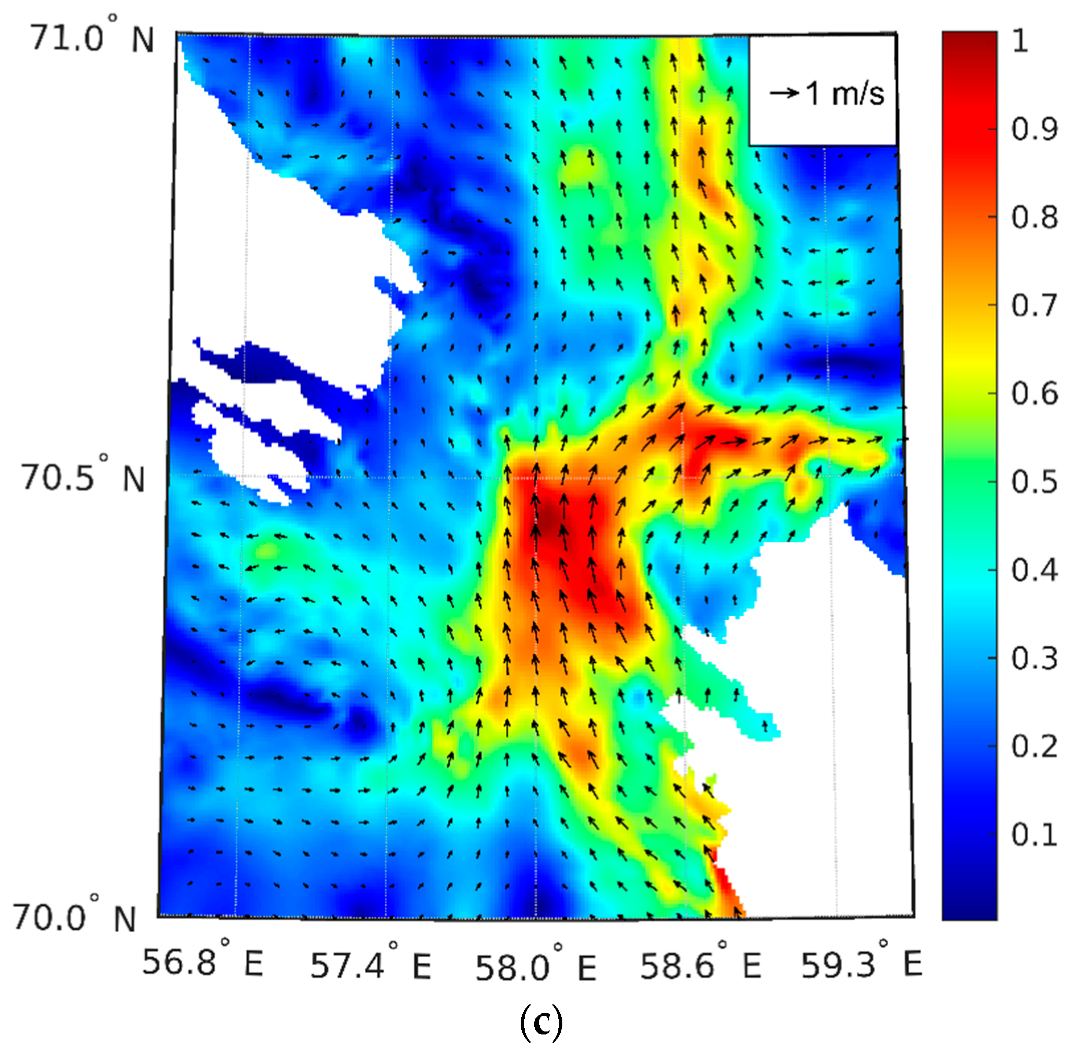
Figure 4.
Tidal conditions in the KG in August 2021 from Arc5km2018 model: (a) tidal variations of sea level [m] on 5-19 August with a red box accenting the period of in situ measurements, while red and green dots showing the start and end of stations; (b) tidal currents (four semidiurnal and four diurnal components) and M2 tidal ellipses predicted by Arc5km2018 model on 12-13 August 2021. Red markers show locations of oceanographic stations.
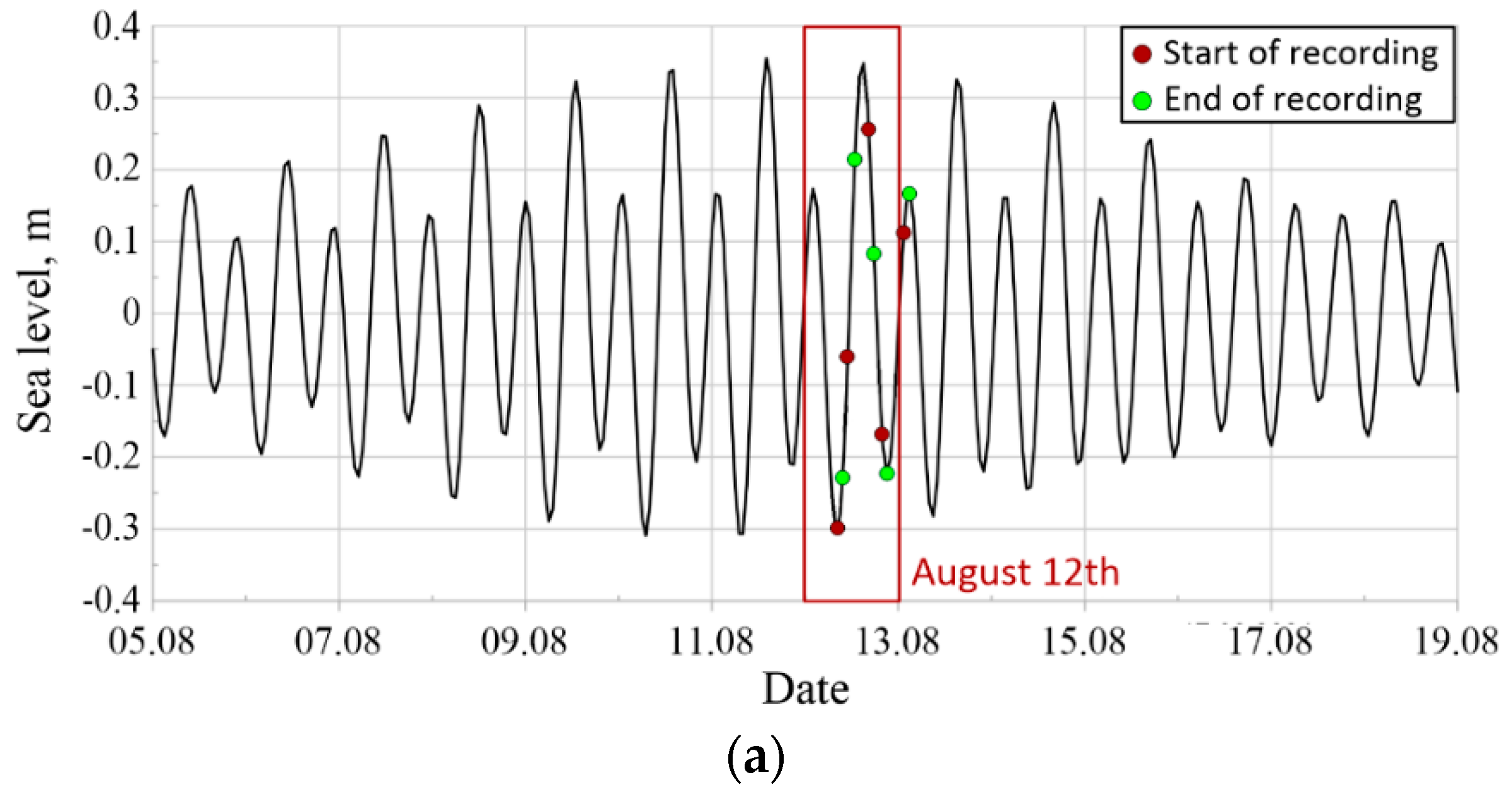
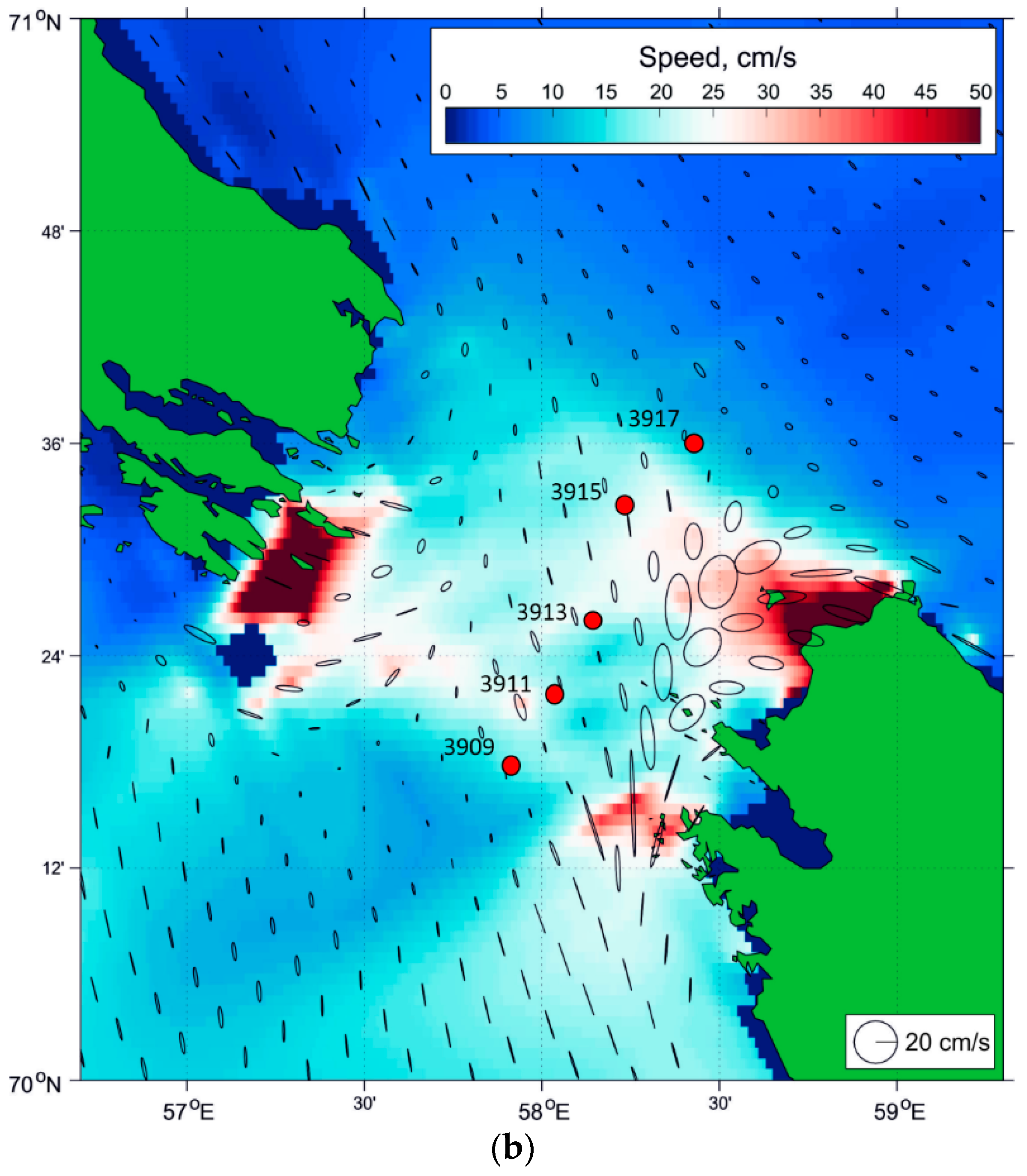
Figure 5.
Surface signatures of NLIWs in Sentinel-2A image of the Kara Gates acquired on 8 August 2021 (08:16 GMT): (a) RGB composite map; (b) enlarged fragment of Band 4 (665 nm) of the central KG strait area marked by white rectangle in (a) with distinct signatures of NLIW trains. Start and end points of oceanographic stations are shown by red and green circles, respectively.
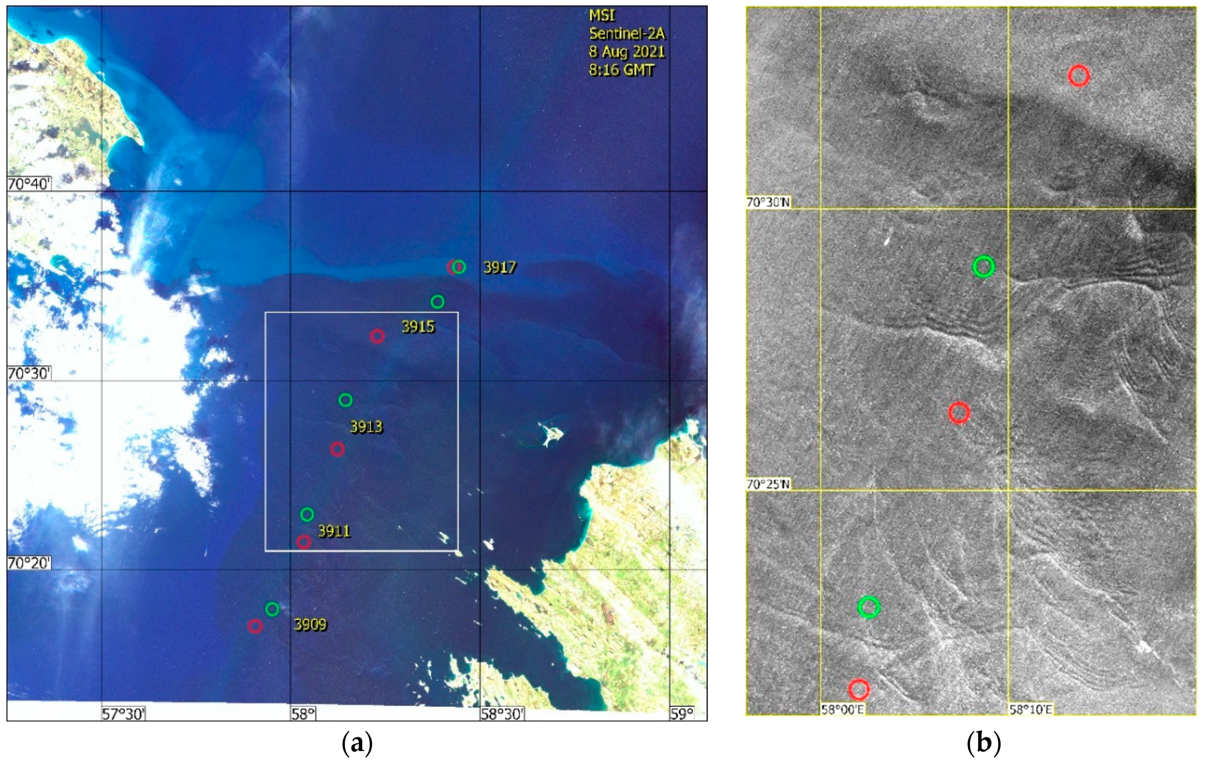
Figure 6.
SAR-C snapshots of the Kara Gates acquired on: (a) 12 August 2021 (02:43 GMT) by Sentinel-1B; (b) 13 August 2021 (02:36 GMT) by Sentinel-1A. Red square in (b) marks the ship location.
Figure 6.
SAR-C snapshots of the Kara Gates acquired on: (a) 12 August 2021 (02:43 GMT) by Sentinel-1B; (b) 13 August 2021 (02:36 GMT) by Sentinel-1A. Red square in (b) marks the ship location.
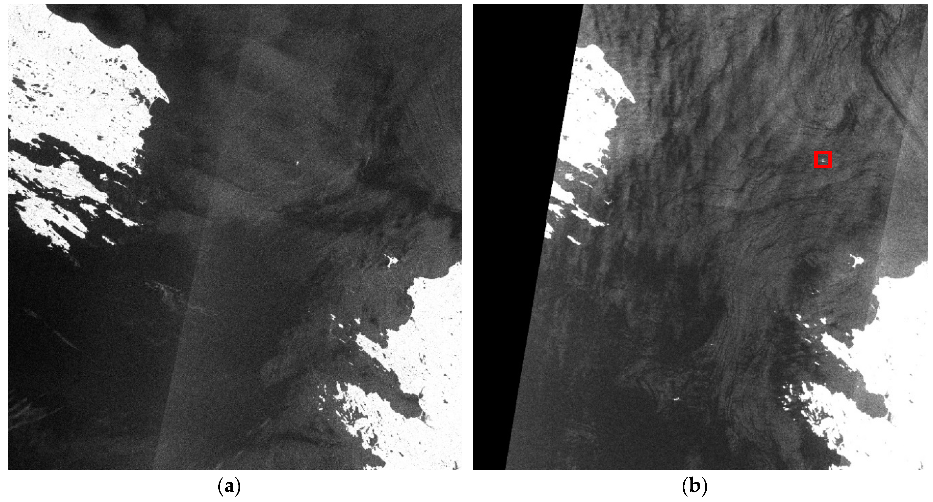
Figure 7.
Oceanographic measurements in the western part of the KG at station 3909 on 12 August 2021: (a) vertical CTD profiles of temperature (red line), salinity (blue line) and buoyancy frequency (black line); (b) time variations of vertical distribution of water temperature from the TPArctic profiling; (c) direction and magnitude of tidal current from Arc5km2018 at the beginning (red arrow) and end (green arrow) of the station; (d) sea bottom topography under the drifting vessel during the station.
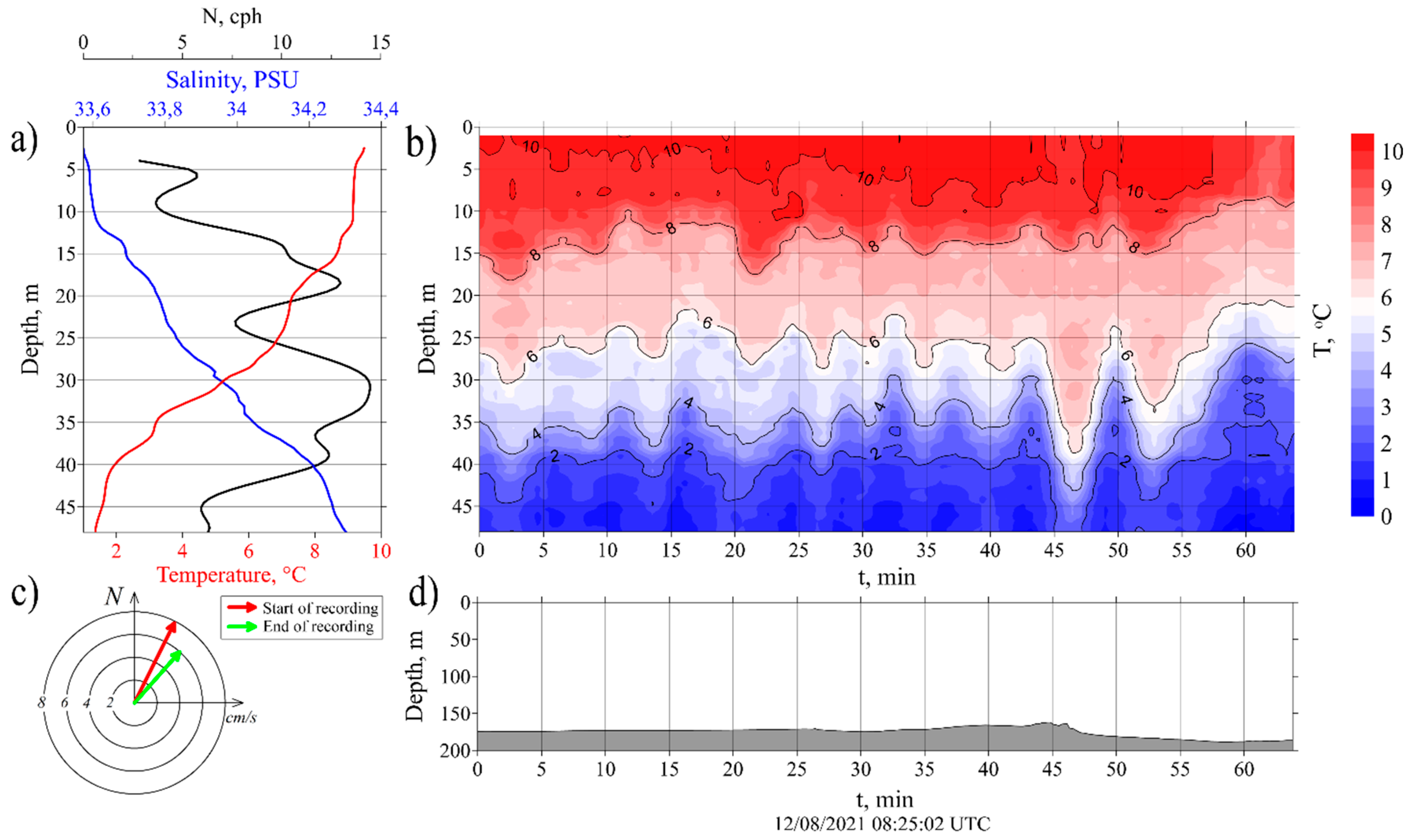
Figure 8.
Oceanographic measurements in the KG at station 3911 on 12 August 2021: (a) vertical CTD profiles of temperature (red curve), salinity (blue curve) and buoyancy frequency (black curve); (b) time variations of vertical distribution of water temperature from the TPArctic profiling; (c) intensity and direction of tidal currents from Arc5km2018 during the start (red arrow) and end (green arrow) of measurements; (d) sea bottom topography under the drifting vessel during the station.
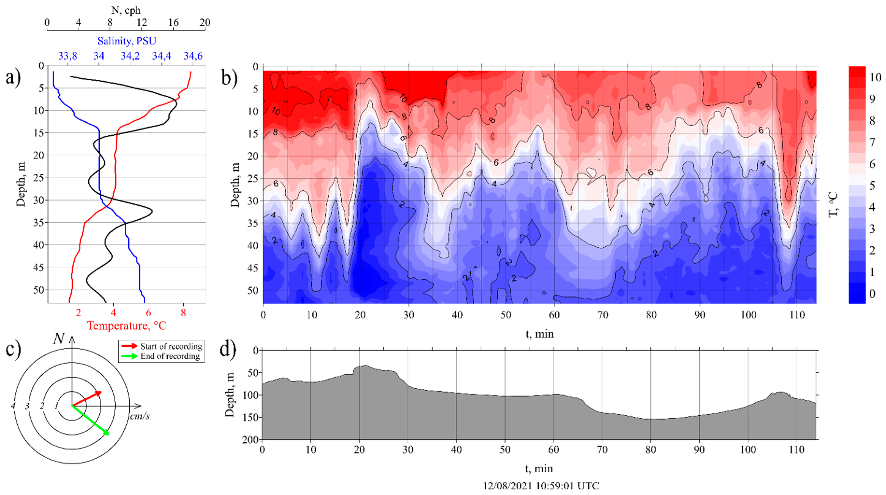
Figure 9.
Aerial view of the KG in the vicinity of station 3911 from UAV showing characteristic narrow slick bands associated with thermocline oscillations. White arrows and dashed yellow curves mark the location of slick bands. Yellow, red and blue arrows show direction to the north, ship drift and IW orientation directions, respectively.
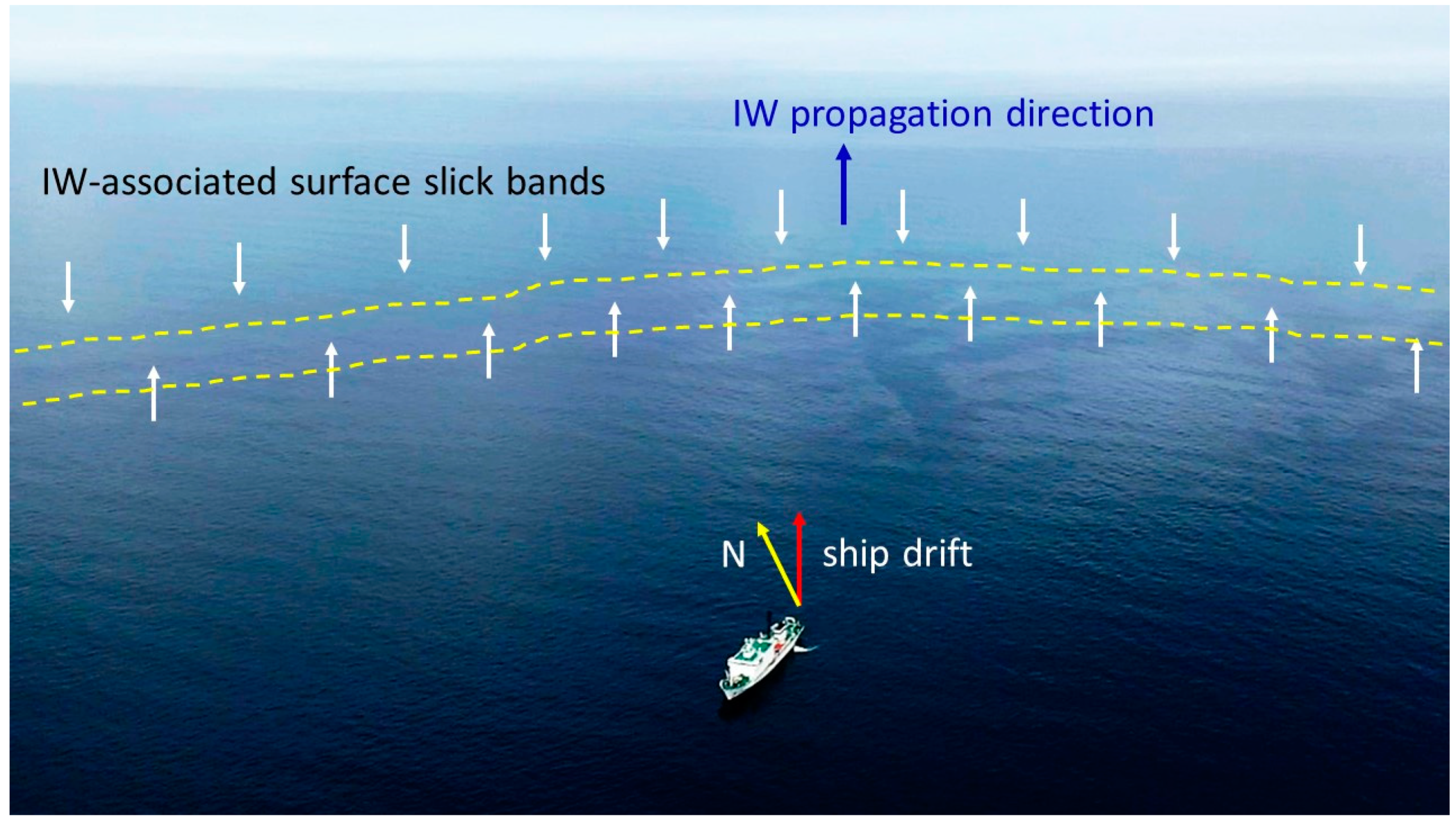
Figure 10.
Manifestation of internal waves in the marine radar records on 12 August 2021 during measurements at station 3911. Blue and red arrow show ship course and drift directions, respectively.
Figure 10.
Manifestation of internal waves in the marine radar records on 12 August 2021 during measurements at station 3911. Blue and red arrow show ship course and drift directions, respectively.
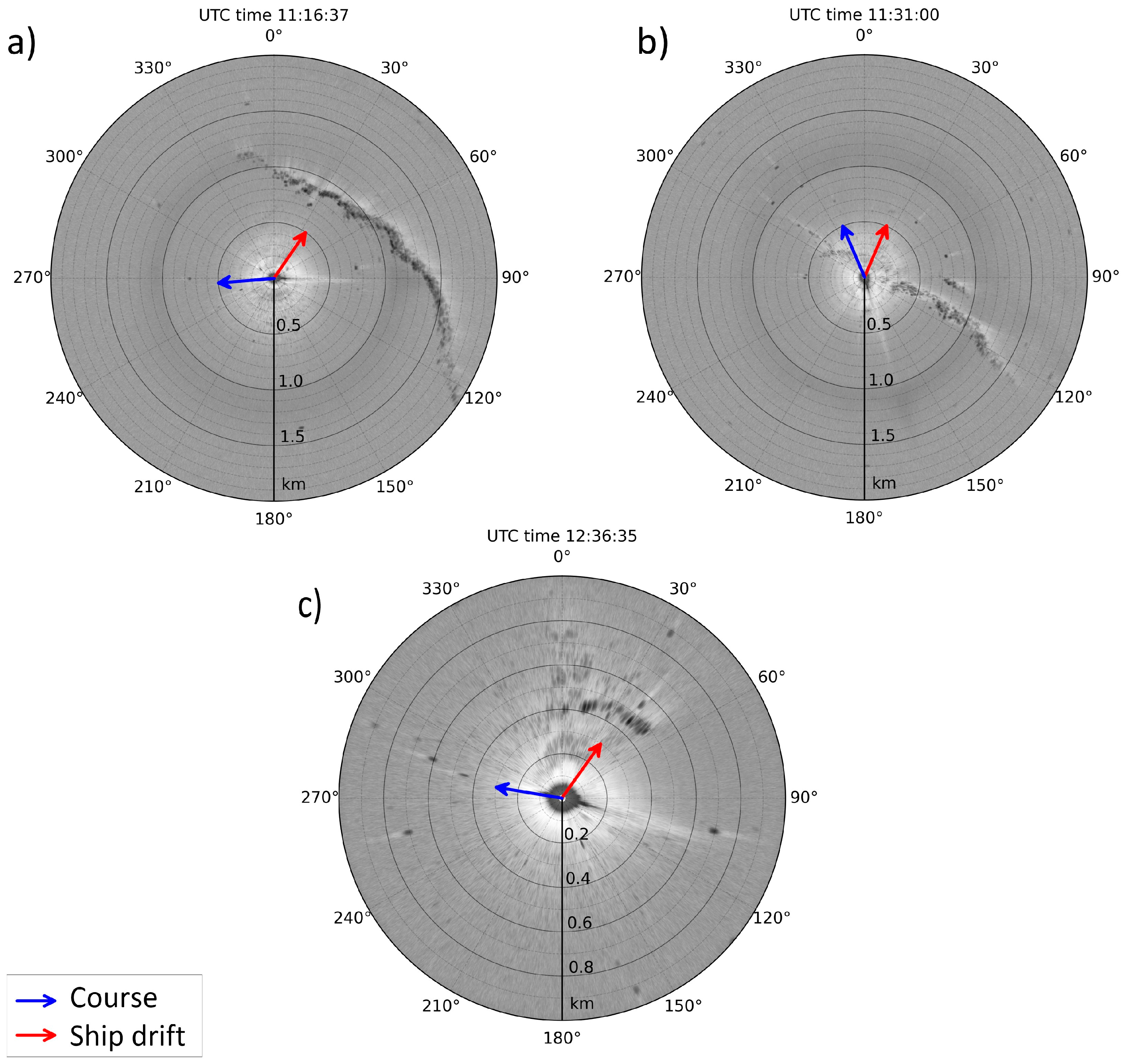
Figure 11.
Oceanographic measurements at station 3913 on 12 August 2021 in the central part of the KG: (a) vertical CTD profiles of temperature (red curve), salinity (blue curve) and buoyancy frequency (black curve); (b) time variations of vertical distribution of water temperature from the TPArctic overlain with selected isopycnals from rapid CTD casts; (c) intensity and direction of tidal currents from Arc5km2018 during the start (red arrow) and end (green arrow) of measurements; (d) sea bottom topography under the drifting vessel during the station.
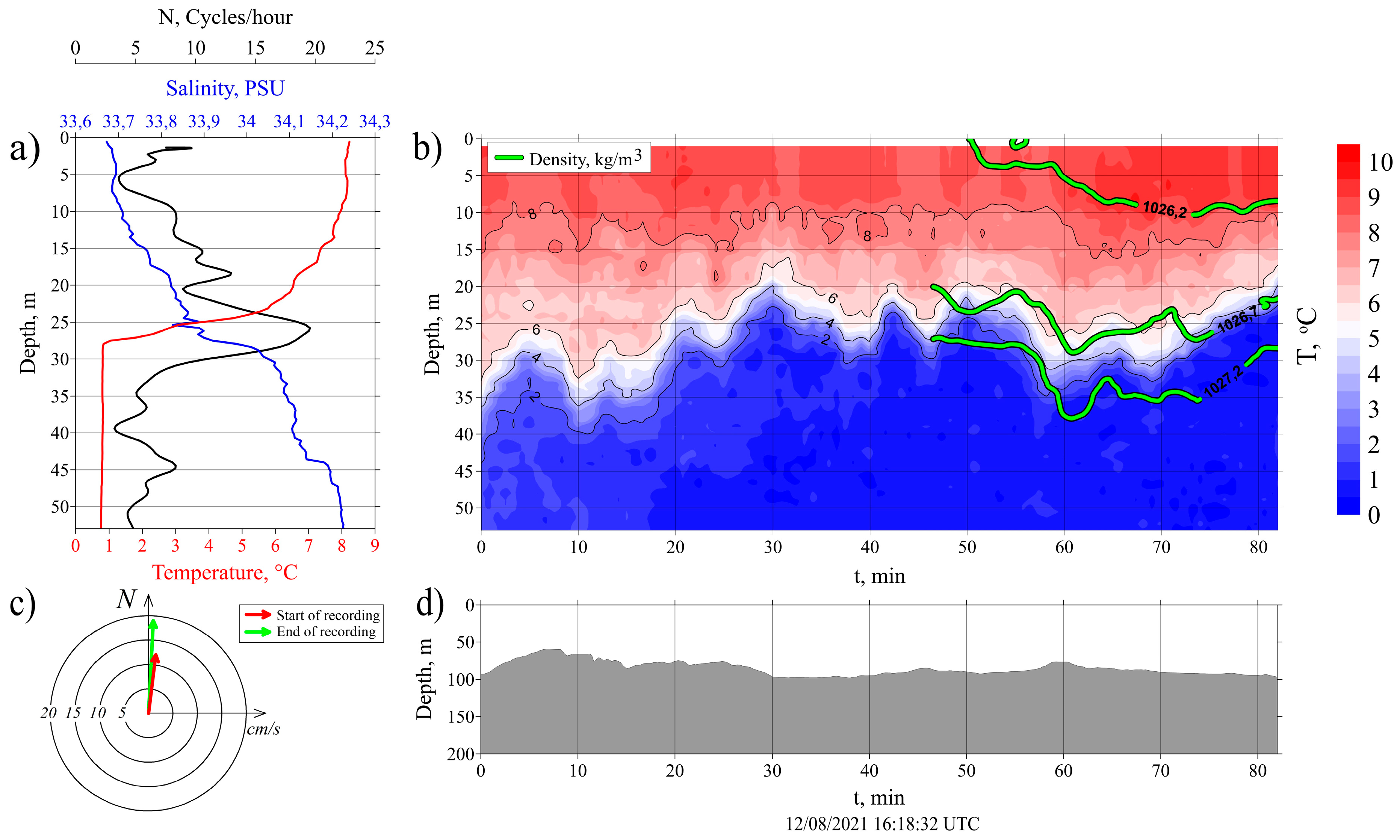
Figure 12.
Oceanographic measurements at station 3915 on 12 August 2021 in the northeastern KG: (a) vertical CTD profiles of temperature (red curve), salinity (blue curve) and buoyancy frequency (black curve); (b) time variations of vertical distribution of water temperature from the TPArctic profiling; (c) intensity and direction of tidal currents from Arc5km2018 during the start (red arrow) and end (green arrow) of measurements; (d) sea bottom topography under the drifting vessel during the station.
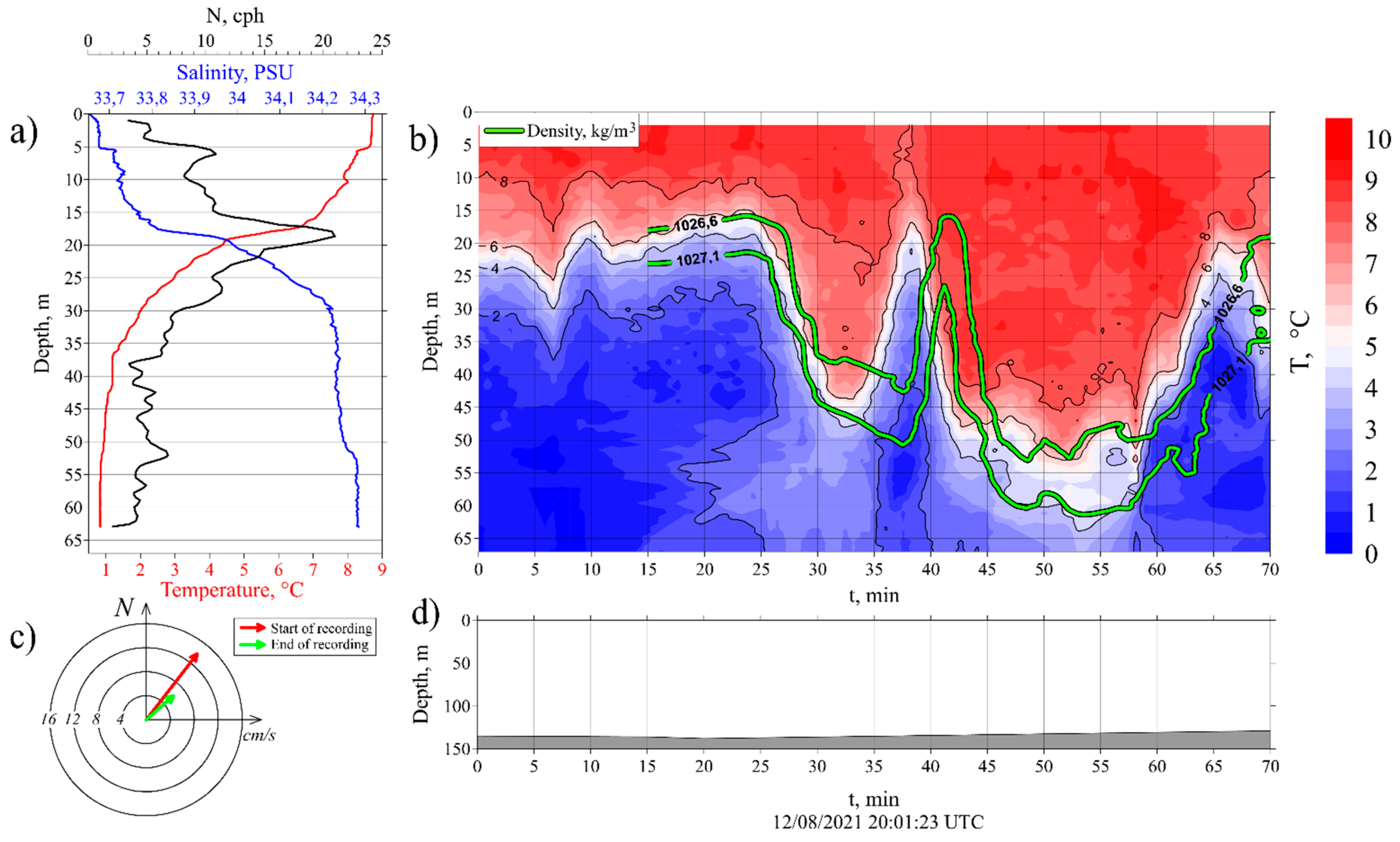
Figure 13.
Internal wave observations at station 3915 on 12 August 2021: (a) time variations of the 7° C isotherm simultaneously recorded by the bow TP (magenta), stern TP (red), TPArctic (blue) and rapid CTD casts (green); (b) aerial view of ship orientation, position of TPs and propagation direction of NLIW relative to the ship; (c) schematic showing ship drift direction (red arrow), NLIW propagation direction relative to the ship (yellow arrow), and the true NLIW propagation direction (blue).
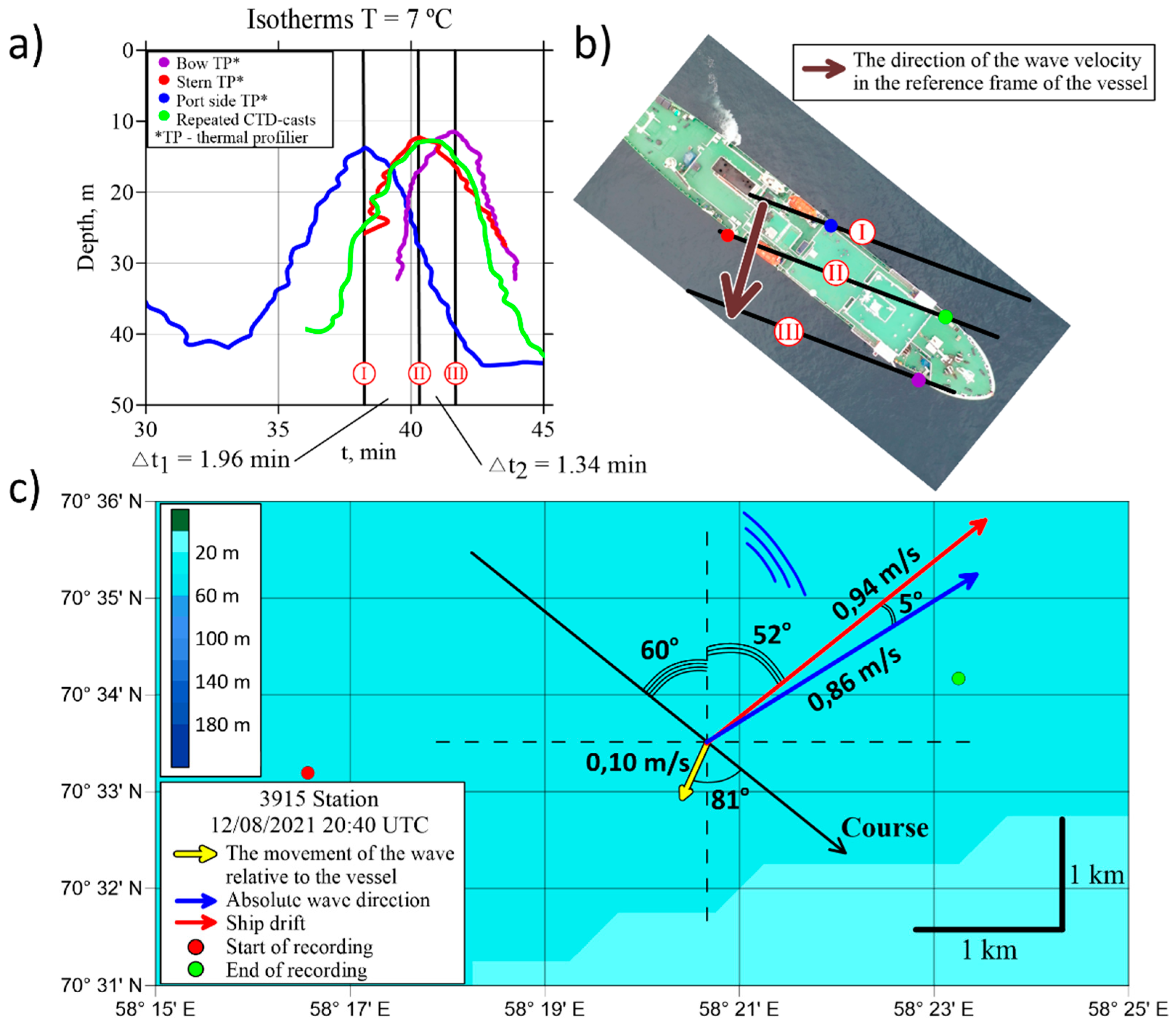
Figure 14.
Surface flow conditions at station 3915: (a) time variations of surface current vector derived from the ship drift (black arrows), and its cross-strait (red line) and along-strait (blue line) components; (b) time variations of the Froude number calculated for 0.42 m/s (cyan line) and 0.54 m/s (dark blue line).
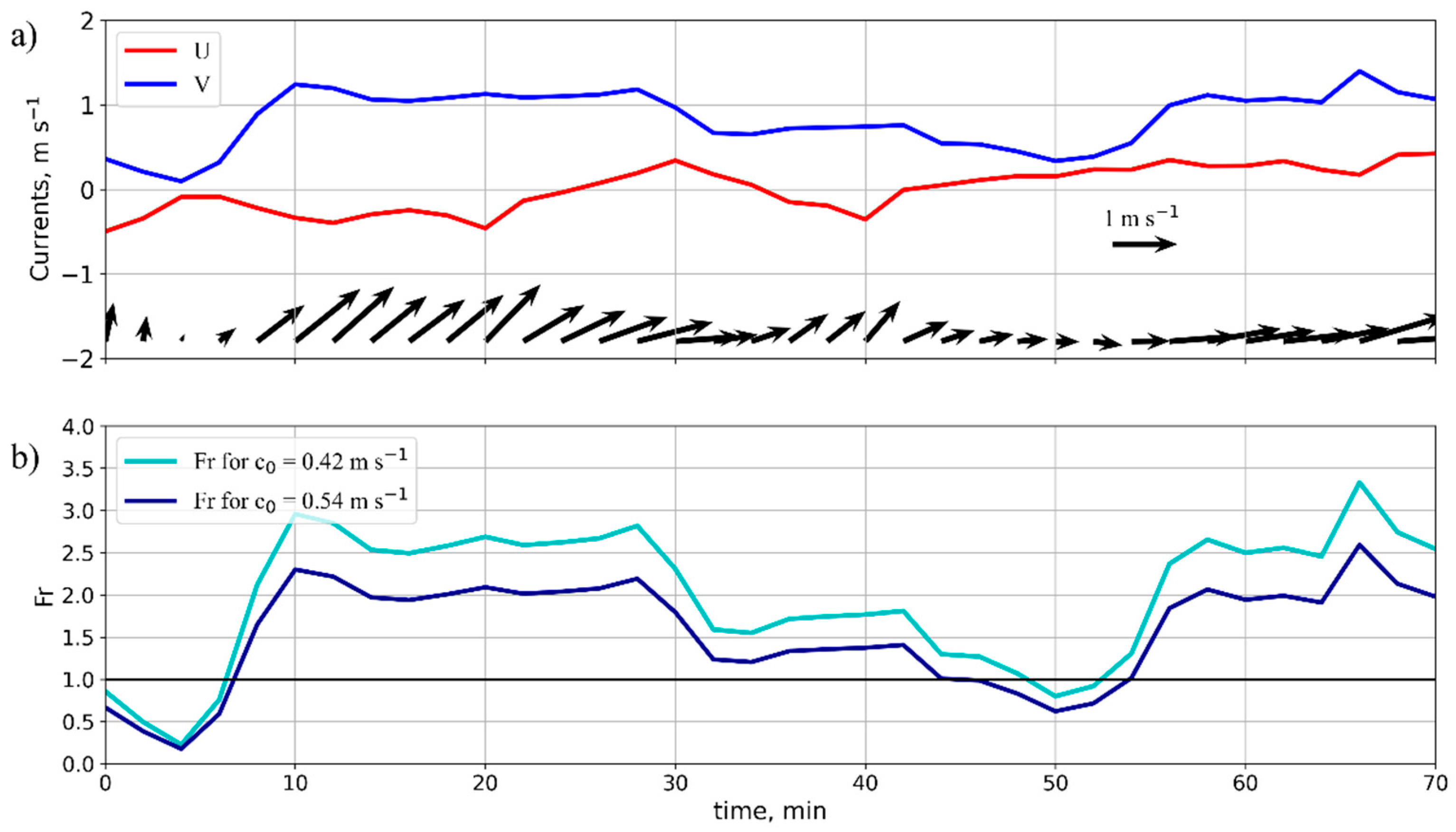
Figure 15.
A generalized scheme of NLIWs’ observations (blue curves) along a system of shallow sills in the Kara Gates superposed with direction of tidal currents (red arrows) during field observations on 12 August 2021.
Figure 15.
A generalized scheme of NLIWs’ observations (blue curves) along a system of shallow sills in the Kara Gates superposed with direction of tidal currents (red arrows) during field observations on 12 August 2021.
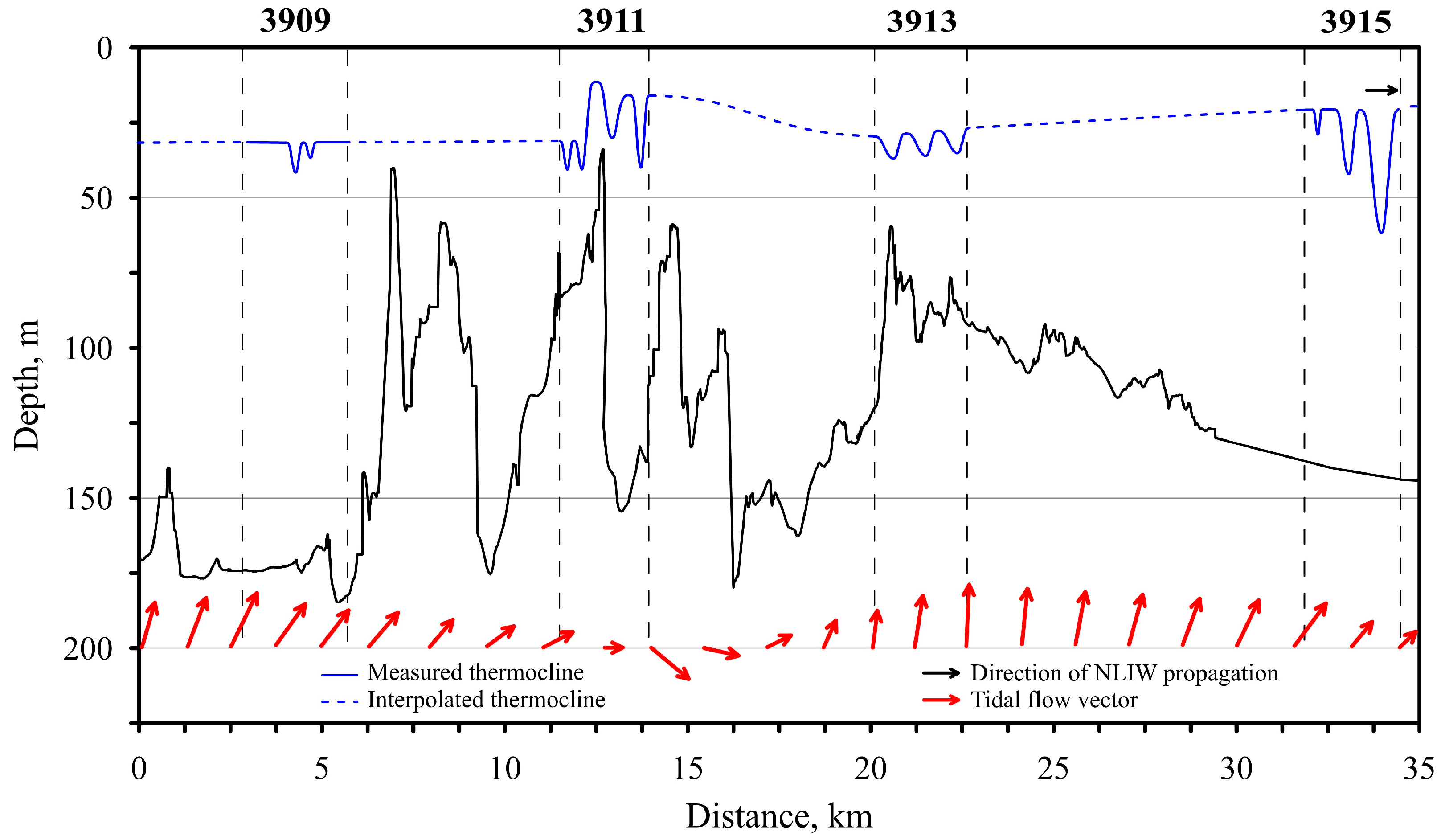

Table 1.
Description of stations made in the KG Strait on 12-13 August 2021.
| Station #; Time | Length of Measurements, h | Start Latitude | Start Longitude | Start Depth, m |
|---|---|---|---|---|
| 3909; 08:25 UTC | 1.1 | 70° 17.292' | 57° 55.797' | 176 |
| 3911; 10:59 UTC | 1.9 | 70° 21.540' | 58° 02.117' | 82 |
| 3913; 16:18 UTC | 1.4 | 70° 26.882' | 58° 07.401' | 131 |
| 3915; 20:01 UTC | 1.2 | 70° 33.275' | 58° 16.586' | 127 |
| 3917; 01:15 UTC | 0.9 | 70° 35.894' | 58° 25.495' | 148 |
Table 2.
Observed and theoretical values of NLIW phase speed at station 3915.
| Parameter | ||||||
|---|---|---|---|---|---|---|
| Eq. # | - | (3), (6) | (3), (4) | (5), (6) | (5), (7) | (5), (9) |
| [m/s] | 0.42 | 0.42 | 0.54 | 0.54 | 0.54 | |
| [m/s] | 0.86 | 0.62-0.7 | 0.62-0.69 | 0.87-0.98 | 0.71-0.72 | 0.73-0.85 |
Disclaimer/Publisher’s Note: The statements, opinions and data contained in all publications are solely those of the individual author(s) and contributor(s) and not of MDPI and/or the editor(s). MDPI and/or the editor(s) disclaim responsibility for any injury to people or property resulting from any ideas, methods, instructions or products referred to in the content. |
© 2023 by the authors. Licensee MDPI, Basel, Switzerland. This article is an open access article distributed under the terms and conditions of the Creative Commons Attribution (CC BY) license (http://creativecommons.org/licenses/by/4.0/).
Copyright: This open access article is published under a Creative Commons CC BY 4.0 license, which permit the free download, distribution, and reuse, provided that the author and preprint are cited in any reuse.


