
Submitted:
16 May 2025
Posted:
19 May 2025
You are already at the latest version
Abstract
The advent of SWOT mission data in combination with the recent altimetry satellites (CryoSat-2, SARAL-AltiKa, Sentinel-3A, Sentinel-3B) provide additional value in regional Dynamic Ocean Topography (DOT) estimation both in the resolution and the accuracy of the final product. The near-real-time records support the phase of the operational altime-try. Two areas in the Western Mediterranean were chosen in order to study the signal and error covariance of each altimetric product from 2017 to 2024. The repeated altimetric tracks were used for the spectral estimation of the signal and error Power Spectral Density (PSD) and covariance. Various covariance models (exponential, Gaussian, ARMA) were tested to fit the data-driven estimation. A similar computation scheme was tested for ma-rine gravity data using simulated repeated fields. The final analytic gravity covariance from the periodogram PSD approach was tested against the fitted empirical one. Finally, gravity and altimetry PSD information is used in the DOT estimation through a tailored Multiple-Input-Multiple-Output-System (MIMOS).
Keywords:
satellite altimetry
; dynamic ocean topography (DOT)
; western mediterranean
; gravity
; multiple-input-multiple-output-system (MIMOS)
; covariance
; power spectral density (PSD)
; SWOT satellite mission
1. Introduction
Remote sensing is nowadays an essential component of the Earth Observation System. New satellite missions provide a value added in environmental monitoring, as the remote part of an integrated with in-situ ground observations system, like the EU Copernicus (https://www.copernicus.eu/en). Radar satellite altimetry has been used for over 50 years for monitoring the sea level and gravity field on a global or regional scale [1]. The last 20 years satellite altimetry has been transformed into its operational phase [2] with near-real-time products that can be used in, e.g., oceanography [3,4,5], gravity field reconstruction [6,7,8,9], hydrology [10,11,12] and height system unification [13,14,15,16].
The use of satellite altimetry in mean Dynamic Ocean Topography (DOT) or Mean Dynamic Topography (MDT) estimation requires accurate information on the gravity field [17]. The advent of SWOT satellite mission data in combination with the recent satellites of Copernicus program (Sentinel satellites) as well as other satellites (e.g., CryoSat-2) can ensure the adequate accuracy and resolution of the final product. Global as well as regional models of DOT can be computed using various methods, e.g., by merging information from altimeter data, GRACE and GOCE gravity field and oceanographic in situ measurements through a filtering procedure [18], by minimizing a global cost function [19], using an optimal filtering technique using least-squares from a Mean Sea Surface (MSS) and the geoid information from GOCE [20], applying spherical harmonic expansion algorithm in a global product estimation [21]. Input-Output System Theory was introduced in gravity field modelling by Sideris [22], while the extension to the Multiple-Input-Multiple-Output System (MIMOS) theory in DOT estimation was presented in [23]. Since then, many issues in the application of the method were resolved, e.g., the sensitivity of the method in the input error, the kernel representation, the data resolution and the Global Geopotential Model (GGM) expansion [24], the resolution of the final product [25], the noise consideration in the repeated altimetric observations [23] and the incorporation of GOCE gravity field information in the estimation procedure [26]. In addition, the method has been applied in various areas, e.g., the Atlantic Ocean [23], the Eastern Mediterranean Sea [26] and the Central Mediterranean Sea [27]. The final estimated mean DOT and the respective geostrophic circulation components can be compared with purely oceanographic in-situ data [26,27] for validation purposes. The major disadvantage of MIMOS theory application to DOT estimation is the noise of the gravity field observations. The gravity anomaly error Power Spectral Density (PSD) can be computed from simulated noise fields or following other simulation approaches [22,23,24,25,26,27].
In this study, two areas in the Western Mediterranean Sea are chosen to investigate the signal and the error covariance of the altimetric data (CryoSat-2, SARAL-AltiKa, Sentinel-3A and 3B) from 2017 to 2024. The signal and error PSD of each mission is computed taking advantage from the successive information of the altimetry data. A similar computation scheme is tested for the gravity information. Various analytical models are fitted into the data-estimated covariances and the annual mean DOT is determined through MIMOS. In addition, the first year of SWOT data contribution and the estimation of first year SWOT signal and error PSD and covariance are considered. Special attention is given to the investigation of the effect of gravity signal and its error from PSD in MIMOS annual mean DOT approximation using either estimated or random information.
2. Data Used and Preprocessing
2.1. Areas Under Study
Two areas were chosen in the Western Mediterranean Sea. AREA A is the sea part before the Strait of Gibraltar. This area is at the border between the Mediterranean Sea and the Atlantic Ocean and is characterized by complex geological and geodynamical features [28,29,30]. AREA B covers the main part of the Western Mediterranean Sea between the east coast of Spain, the islands of Corsica and Sardinia, the northern coast of Africa and the south shoreline of Italy and France. The areas under study are depicted in Figure 1 (AREA A: -6° ≤ λ ≤ 0° and 34° 30΄ ≤ φ ≤ 37° 30΄; AREA B: 0° ≤ λ ≤ 9° and 36° ≤ φ ≤ 44°).
2.2. Data
Seaborne gravity anomalies collected during the GEOMED 2 project [31,32] were used for the retrieval of the gravity field information in both areas. These data sets were part of Morelli, BGI and SHOM databases which were processed and edited under GEOMED 2 [32]. 48195 point gravity anomalies for AREA A and 260205 values for AREA B were finally chosen. The data distribution for both areas is depicted in Figure 2a – AREA A and in Figure 2b – AREA B. As it is noted in Tziavos [32], seaborne gravity data of GEOMED 2 project have an a-posteriori sd ranging from 2 to 5 mGal according to numerous editing tests (debiasing, crossover adjustments, comparison with altimetry derived gravity, etc.).
Altimetry data sets from SARAL/AltiKa, CryoSat-2, Sentinel-3A, Sentinel-3B and the first year of SWOT satellite were collected from AVISO website (https://www.aviso.altimetry.fr/en/home.html). The L2P version 4 non-time-critical processed data (Sea Surface Heights – SSHs) [33,34] were confined to the areas under study. The SSHs were computed by the addition of the Mean Sea Surface (MSS) to the Sea Level Anomaly (SLA) product delivered by AVISO. Especially for SWOT, the L3_LR_SSH Expert product [35] was utilized because it is consistent with the other satellites. All altimetric data were referenced to the WGS84 ellipsoid and the zero-tide system.
2.3. Preprocessing
An important step before the PSD signal and error estimation is the smoothing of the data. In gravity field modelling this smoothing can be achieved using long wavelength information from a global geopotential model. The removal of these gravity features lead to smoother potential field, ready for appropriate gridding before spectral calculations. The seaborne gravity anomalies were reduced to the XGM2019 [36] reference geopotential model expanded to degree and order 2190. The statistics of the reduced gravity anomalies after the removal of the contribution of the geopotential model are presented in Table 1 for AREA A and in Table 2 for AREA B.
3. Results – Discussion
3.1. Empirical and Analytical Gravity Covariance Models
The empirical covariance of the reduced gravity data was computed using EMPCOV routine from the GRAVSOFT software suite [37]. The resolution for the empirical covariance spacing was chosen equal to 3 arcmin, in accordance to the density of the original data. Four analytical models were tested to fit the empirical values, namely the simple exponential model [38]
where C(ψ) is the empirical covariance value at ψ spherical distance, and a, b are the unknown coefficients of the analytical model; the planar Gaussian model [39]
where C(s) is the empirical covariance value at s horizontal distance, and a, b are the unknown coefficients of the analytical model; the 3rd order Auto-Regressive Moving Average (ARMA) model [40]
where C(ψ) is the empirical covariance value at ψ spherical distance, and a, b and c are the unknown coefficients of the analytical model; the Tscherning – Rapp covariance model [41]
where C(ψ) is the empirical covariance value at ψ spherical distance between the computation point and the data point, a is a scale factor that needs to be estimated, M is the maximum expansion degree of the geopotential model (2190 in our case), εn are the error degree variances of XGM2019, R is a mean earth radius, is the radius of Bjerhammar sphere [42], and are the geocentric distances of points P and Q, Pn are the fully normalized associated Legendre polynomials of degree n and are the anomaly degree variances from the Tscherning–Rapp model [41]. The empirical covariance values as well as the analytical model estimated in each test area are depicted in Figure 5 and Figure 6.
C(ψ) = a·exp(-bψ),
C(s) = a·exp(-s2/b2),
C(ψ) = a·(1+b1ψ+b2ψ2+b3ψ3)·exp(-cψ),
As shown in Figure 5 and Figure 6, the covariances of the two study areas have a correlation length of approximately 0.1 degree. This fact confirms the homogeneity of the GEOMED 2 database which is used in both areas. In addition, AREA A is smaller than AREA B and this is the reason of the different shape in the final empirical covariance figure. Another point of interest is the estimated variance in each area: in AREA A the observed variance was equal to 27.19 mGal2, while in AREA B was found to be 19.45 mGal2.
In order to validate the analytical model fitting procedure, quality measures were used based on the variance of the adjustment (a-posteriori variance), the correlation coefficient [43]
and the misfit coefficient [44]
where is the number of the empirical model covariance values, is the model covariance value at the point, is the empirical covariance value at the same point , is the mean covariance value from the analytical model, is the mean covariance value from the empirical function and is the variance of the fitted analytical model. The results of the computed statistical measures are presented in Table 3 for AREA A and in Table 4 for AREA B.
3.2. Periodogram and Inverse Correlogram Approach for the Gravity Data
The major difficulty in the application of the MIMOS theory in gravity field modelling is the necessity of the input error PSD of the observations. Since only the variance of the observations is known and not the error itself, the direct computation of the observation error PSD is not straightforward. Given that the observation variances change from point to point, the noise is not part of a stationary stochastic process [22,23,45]. This fact complicates the solution in the frequency domain, where the simple algebraic equations are transformed into integral relations [46] and the simplified spectral character is cancelled. Various solutions were proposed for the observation noise statistical information as the simulation of random noise field [47], stationary simulation models of the input error PSD [48,49] and the PSD estimation from successive measurement information, as in the case of satellite altimetry [23,45,50].
A similar approach was tested for the gravity measurements in both areas under study. Gravity information was divided into ten (10) randomly distributed fields in order to evaluate the PSD estimation from the data (periodogram approach). The random division of the gravity information has of course an inherent simulation assumption. Nevertheless, since the original data records were not available, as well as the measurement procedure and the date of each campaign, the division into ten gravity fields randomly was the only possibility in the periodogram approach. The randomly distributed gravity field selection scheme is depicted in Figure 7.
The randomly divided gravity fields were gridded using adjustable tension continuous curvature splines [51] by surface and blockmean modules of the Generic Mapping Tools version 6 [52]. The grid spacing was chosen equal to 3 arcmin and the tension factor to 0.25. Using the multiple gravity field information, a similar to the successive altimetric data algorithm [23] was followed. Each gravity observation field is divided into the unknown signal and noise information:
where is the gravity anomaly observation at a specific grid point, k+1 is the number of the successive field information (in our case k+1=10), is the unknown gravity anomaly signal at the specific grid point and is the unknown gravity anomaly observation error (i = 1,…,k+1). Transforming the grids into the spectral domain and subtracting each gravity field from the successive one, the gravity anomaly error PSD estimation is derived:
where and are the spectra of the gravity observations and noise at the i cluster field. The mean gravity anomaly error PSD can be estimated using the spectral properties of the periodogram approach [23,50]:
where is the mean gravity anomaly error PSD, and * denotes the complex conjugate of the spectrum. In a similar manner, the estimation of the mean gravity signal PSD is computed:
where is the spectrum of the unknown gravity anomaly signal. The mean gravity signal PSD can be derived using the complete successive gravity information:
The estimation of the gravity signal and error covariance functions can be derived using the computed PSD information. The inverse correlogram approach (PSD estimation from the covariance using FFT) can be applied to the 2D signal and error gravity PSDs. It is needed to note here that the inverse correlogram approach transforms originally the PSD into the correlation function. Since the gravity anomaly observations were reduced to a global GGM (see Section 2.3), the inverse correlogram approach leads to the estimation of the covariance function [53,54]. The mean gravity signal covariance can be estimated using the inverse FFT operator F-1:
and the mean gravity error covariance:
The 2D gravity signal and error covariances derived from the inverse correlogram approach were averaged over azimuth in order to estimate the 1D isotropic covariances and test the analytical model fitting procedure. The simple exponential and 3rd order ARMA analytical models from Section 3.2 were used for fitting the empirical data estimated from the periodogram and inverse correlogram approach. The empirical as well as the analytical model for the signal and error gravity anomaly covariances are depicted in Figure 8 for AREA A and Figure 9 for AREA B.
As seen in Figure 8 and Figure 9, the 3rd order ARMA analytical model provided the best fitting results in the signal covariance. In the error covariance fitting, ARMA as well as the simple exponential model gave comparable results. The quality measures for the fitting procedure are presented in Table 5 for AREA A and in Table 6 for AREA B.
3.3. Comments on the Gravity Anomaly Covariance Estimation Schemes
Comparing the empirical values of the covariances derived from the classical gravity anomaly observations cluster procedure using EMPCOV [37] and the data-driven periodogram PSD estimation and inverse correlogram approach various issues can be pointed out. The signal covariance derived from the inverse correlogram approach seems smoother than the classical empirical one derived from the observations. We must note here that the inverse correlogram approach leads to the signal covariance estimation, while the classical estimation computes an observation (signal and error) covariance. Of course, the PSD-derived covariance can be estimated under certain assumptions, e.g., the random observation separation (ignoring the exact campaign date) and the noise stationarity hypothesis. The variance of the classical empirical covariance in AREA A was estimated equal to 27 mGal2 while in the inverse correlogram approach was 36 mGal2. On the contrary, in AREA B the variances of the classical and the PSD-driven procedure were computed 19 mGal2 and 6.2 mGal2, respectively. In addition, the correlation length of the PSD-derived covariances is shorter than the classical estimated covariances in both areas and drops from 0.1 degrees to 0.05 degrees. This fact can be attributed to the signal covariance estimation procedure that uses the abovementioned assumptions. The random observations separation and the stationarity assumption tend to a Dirac-type covariance estimation and reduce the correlation length.
3.4. Satellite Altimetry PSDs and Covariance Estimation
Satellite altimetry data from 2017 to 2024 were utilized similarly to the gravity approach for the signal and noise PSD and covariance estimation. The repeated altimetric tracks provide a multiple sample configuration. Using this information, a PSD estimation is possible. Following [50] and [23], the observed corrected Sea Surface Height (SSH) can be derived as
where hi is the observed corrected SSH, i = 1,…,k+1 is the number of repeated tracks, h is the time-invariant part of the altimetric observation equation (marine geoid plus mean DOT), Δζi is the time-variant part of the DOT, and ni is the altimetric observation noise. The environmental, geophysical and orbit corrections described in [34] and [35] were applied in order to estimate the corrected SSH. Assuming that Δζi follows a random distribution and no correlation between Δζi and ni exists, then a new random variable ei can be assigned by
hi = h + Δζi + ni ,
ei = Δζi + ni .
This new variable incorporates the statistical information of the observation noise, as well as the assumed random time-variant part of the DOT. Of course, as shown in [50] and [23], this assumption is not exactly valid in the case of slow-moving oceanographic features; in this case aliasing effects can be incorporated into the oceanic geoid signal.
Repeated altimetric data from CryoSat-2, SARAL/AltiKa, Sentinel-3A and 3B as well as the first year of SWOT data were used. The estimation of the mean yearly 2D signal and error covariance was based on the procedure presented in [23], i.e., data periodogram and inverse correlogram approach. The final 2D covariances were averaged over azimuth in order to compute the isotropic ones. The same, as in the gravity data processing, analytical models were tested in the altimetry case. The estimated yearly satellite altimetry signal and noise covariances for the year 2017 are depicted in Figure 10. SARAL/AltiKa, CryoSat-2 and Sentinel-3A were active at that time. The SSH signal variance is comparable for all the investigated satellites at the order of 1.8 m2. For the error variances, Sentinel-3A data led to 0.33 cm2 while SARAL/AltiKa and CryoSat-2 error variance were computed at the 6.5 and 8.2 cm2 level, respectively. This difference can be attributed to the better performance of Sentinel-3A instrumentation, something that can be confirmed during the whole study period.
In Figure 11, the yearly signal and error altimetry covariance for the first semester of 2024 are presented. For the first semester of 2024, all altimetry satellites (CryoSat-2, SARAL/AltiKa, Sentinel-3A, Sentinel-3B, SWOT) led to similar SSH signal covariances with a variance of 0.42 m2, approximately. A slightly lower variance was estimated for the SWOT data, namely 0.33 cm2. Different behavior can be seen in the SSH noise covariance estimation: SARAL/AltiKa and CryoSat-2 presented a variance of 7.5 cm2, while the Sentinels led to an order of magnitude less estimation (0.18 cm2 for Sentinel-3A and 0.55 cm2 for Sentinel-3B). The magnitude of the noise in the Sentinels is consistent over all the period of study (2017 – 2024) and confirms the quality of the altimetric instrumentation and the accurate preprocessing of the data.
Different behavior for the noise is depicted in Figure 11 regarding SWOT altimetric data. The noise variance of the first semester of 2024 for SWOT was estimated to 22 cm2, a magnitude larger than the noise variances of SARAL/AltiKa and CryoSat-2. This fact can be attributed to the initial phase of the satellite. In order to confirm this behavior, the whole 1st year of SWOT data signal and noise covariance was analyzed. Cycles 1 to 17 of SWOT altimetry data (July 2023 – June 2024) were processed in order to estimate 2D signal and noise PSD and covariance. In Figure 12 (a) and (b) the signal and noise covariances for the first year of SWOT data in AREA A and AREA B are presented, respectively. The error variance in both areas was computed larger of one order of magnitude than the other satellites confirming the results shown in Figure 11. The different instrumentation, the initial phases of the satellite and the special measurement principle (SAR altimetry [55]) can probably affect the error covariance estimation. This will be the subject of another study, where more than 3 years of SWOT will be available and thus more reliable conclusions could be drawn.
3.5. MIMOS Yearly Mean DOT Estimation
Yearly steady mean DOT was estimated through MIMOS following the algorithm presented by Andritsanos et al. [23]. The altimetry estimated signal and error PSD were used in the procedure. In the case of gravity anomaly data, simulated (random noise of 5 mGal sd) as well as estimated PSD (see Section 3.3) were utilized to examine the effect of the estimated noise to the final yearly mean DOT. The final annual mean DOT for the year 2023 using real estimated gravity PSD is depicted in Figure 13a for AREA A and 13b for AREA B. It is noticed that the values near the coastlines are not accurate due to the lack of enough gravity data and the inherent problems of altimetric data in shallow waters.
The differences in the annual DOT estimation using real estimated gravity PSD versus random gravity noise for the year 2017 and 2024 are depicted in Figure 14 and Figure 15. The differences between the two solutions are minor and the major values are found near the coastlines due to the lack of gravity data. The simulated versus the real data input gravity PSD performed equally in the final mean DOT estimation. The sensitivity of the input data noise to the final MIMOS estimates is studied in [24]. In both areas, the estimated input gravity PSD/covariance led to similar DOT output variance w.r.t. the simulated one.
The estimated 2D and averaged 1D mean DOT output covariances are presented in Figure 16 for 2017 in AREA A and in Figure 17 for 2023 in AREA B.
As shown in Figure 16 the variance of the output error annual mean DOT for the year 2017 in AREA A was estimated 2.6 cm2 and 2.8 cm2 for simulated input gravity noise and real data estimated PSD, respectively. In addition, considering Figure 17, the output variance was computed 1.7 cm2 using simulated gravity noise, while in the real data estimated PSD the value was 1.1 cm2. On the other hand, as shown in Figure 16 and Figure 17, the computed output annual mean DOT error covariances showed larger correlation length than the simulated ones. The use of simulated random gravity noise led to a spike-like DOT output error covariance.
4. Summary and Conclusions
Signal and error gravity and altimetry PSD and covariance studies in two areas in the Western Mediterranean Sea were presented in this work. Gravity data from GEOMED-2 project were combined with altimetry data from CryoSat-2, SARAL/AltiKa, Sentinel-3A, Sentinel-3B and the first year of SWOT data through a MIMOS scheme in order to estimate yearly mean DOT.
The gravity anomaly covariance was modelled using the classical empirical estimation and the analytical model fitting. A 3rd order ARMA analytical model yielded the best empirical fitting according to proper statistical measures. In the second test, a successive algorithm for estimating the gravity anomaly signal and error PSD using periodogram approach was used. Due to the lack of gravity campaign and date information, randomly selected fields were constructed and the successive algorithm led to the signal and noise covariances derived directly from the data using inverse correlogram approach. The 3rd order ARMA analytical model led to better fitting than the other models (simple exponential, gaussian, etc.) in the signal covariance modelling, while a simple exponential model seemed to fit better in the noise covariance adjustment. The signal covariance derived from the inverse correlogram approach seems smoother than the classical empirical one derived from the observations. Of course, the PSD-derived covariance can be estimated under certain assumptions, e.g., the random observation separation due to the lack of the campaign date and the noise stationarity hypothesis. In addition, due to the abovementioned assumptions, the correlation length of the PSD-derived covariances is shorter than that of the classical covariances.
Satellite altimetry data from 2017 to 2024 were tested in a similar manner for signal and noise PSD and covariance estimation. Repeated altimetric data from CryoSat-2, SARAL-AltiKa, Sentinel-3A and 3B as well as the first year of SWOT data were used. The estimation of the mean yearly 2D signal and error covariance was based on the data periodogram and inverse correlogram repeated algorithm approach. The signal SSH variance is comparable for all the investigated satellites, while for the error variances the Sentinels performed better than SARAL/AltiKa and CRYOSAT. This fact can be attributed to the better performance of the Sentinels’ instrumentation, something that can be confirmed during the whole study period. An interesting time period is the first semester of 2024, when all tested altimetry satellites were active. The data from the recently launched mission of SWOT led to a slightly lower variance in the SSH signal covariance than the other operated satellites. An interesting part of the study is the estimation of the SWOT SSH noise covariance: the noise variance of the first semester of 2024 was estimated a magnitude larger than the noise variance of SARAL/AltiKa and CryoSat-2. This fact can be attributed to the initial phase of the satellite. In order to confirm this behavior, the whole 1st year of SWOT data signal and noise covariance was analyzed and the abovementioned conclusion on the SWOT data error budget was justified. Of course, more reliable conclusions can be drawn after the 3rd year of complete mission data collection.
Using the statistical information of the gravity and altimetry observations a MIMOS scheme was utilized for estimating yearly mean DOT in the areas under study. In the case of gravity anomaly data, simulated as well as estimated PSD were utilized in order to examine the effect of the estimated noise in the final yearly mean DOT. The differences between the two solutions were minor with the larger values being found near the coastlines due to the lack of gravity data. The simulated versus the real data input gravity PSD performed equally in the final mean DOT estimation. On the other hand, the computed output annual mean DOT error covariances were more sensitive to the use of random or estimated input gravity noise focusing on the different correlation length. The use of simulated random gravity noise led to a spike-like DOT output error covariance.
A final remark goes to SWOT altimetry mission. A thorough study of the newly available SWOT data is needed with special attention to its advanced measurement approach. The nadir along track measurements of the classical altimetric procedure can be combined with the swath-based data towards the signal and error PSD estimation. The generic swath grid can be used in a direct PSD estimation without the smoothing of the gridding procedure of the along track observations.
Author Contributions
Conceptualization, V.A. and I.T.; methodology, V.A.; software, V.A.; validation, V.A., V.G. and I.T.; formal analysis, V.A.; investigation, V.A. and I.T.; resources, V.A. and V.G.; data curation, V.A., V.G. and I.T.; writing—original draft preparation, V.A.; writing—review and editing, V.G. and I.N.; visualization, V.A. and V.G. All authors have read and agreed to the published version of the manuscript.
Funding
This research received no external funding.
Conflicts of Interest
The authors declare no conflicts of interest.
Abbreviations
The following abbreviations are used in this manuscript:
| DOT | Dynamic Ocean Topography |
| MIMOS | Multiple Input – Multiple Output System |
| ARMA | Auto-Regressive Moving Average |
| PSD | Power Spectral Density |
| EU | European Union |
| MDT | Mean Dynamic Topography |
| MSS | Mean Sea Surface |
| GGM | Global Geopotential Model |
| SSH | Sea Surface Height |
| SLA | Sea Level Anomaly |
| FFT | Fast Fourier Transform |
References
- Rummel, R.; Sansò, F. eds. Satellite Altimetry in Geodesy and Oceanography; Lecture Notes in Earth Sciences; Springer-Verlag: Berlin, 1993.
- Benveniste, J.; Ménard Y. Taking the Measure of Earth. Fifteen Years of Progress in Radar Altimetry; ESA bulletin 128; 2006.
- Le Traon, P.-Y.; Dibarboure, G.; Lellouche, J.-M.; Pujol, M.-I.; Benkiran, M.; Drevillon, M.; Drillet, Y.; Faugere, Y.; and Remy, E. Satellite altimetry and operational oceanography: from Jason-1 to SWOT; EGUsphere [preprint]; 2025. [CrossRef]
- Schiller A.; Brassington, G.B. eds. Operational oceanography in the 21st Century; Springer: Dordrecht, Heidelberg, London, New York; [CrossRef]
- Venkatesan, R.; Tandon, A.; D’ Asaro, E.; Atmanand, M.A. eds. Observing the Oceans in Real Time; Springer International Publishing: Switzerland; [CrossRef]
- Li, Z.; Guo, J.; Ji, B.; Wan, X.; Zhang, S. A Review of Marine Gravity Field Recovery from Satellite Altimetry. Remote Sens. 2022, 14, 4790. [CrossRef]
- Hwang, C.; Hsu, HY.; Deng, X. Marine Gravity Anomaly from Satellite Altimetry: a Comparison of Methods over Shallow Waters. In: Hwang, C., Shum, C.K., Li, J. (eds) Satellite Altimetry for Geodesy, Geophysics and Oceanography. International Association of Geodesy Symposia; vol 126; 2003; Springer: Berlin, Heidelberg; [CrossRef]
- Li, Z.; Guo, J.; Zhu, C.; Liu, X.; Hwang, C.; Lebedev, S.; Chang, X.; Soloviev, A.; and Sun, H. The SDUST2022GRA global marine gravity anomalies recovered from radar and laser altimeter data: contribution of ICESat-2 laser altimetry, Earth Syst. Sci. Data 2024, 16, 4119–4135; [CrossRef]
- Li, Q.; Zhai, Z.; Bao, L.; Wang, Y.; Wu, L.; Mao, G; Sun, H. A convolutional neural network to optimize multi-mission satellite altimeter fusion for improving the marine gravity field. Earth Planets Space 2024, 76, 129. [CrossRef]
- Jiang, L.; Zhao, Y.; Nielsen, K.; Andersen O.B.; Bauer-Gottwein P. Near real-time altimetry for river monitoring – a global assessment of Sentinel-3. Environ. Res. Lett. 2023, 18, 074017. [CrossRef]
- Hulsman, P.; Winsemius, H.C.; Michailovsky, C.I.; Savenije, H.H.G.; Hrachowitz, M. Using altimetry observations combined with GRACE to select parameter sets of a hydrological model in a data-scarce region. Hydrology and Earth System Sciences 2020, 24(6), 3331 – 3359; [CrossRef]
- Lee, C.M.; Kuo, C.Y.; Yang, C.H.; Kao, H.C.; Tseng, K.H.; Lan, W.H. Assessment of hydrological changes in inland water body using satellite altimetry and Landsat imagery: A case study on Tsengwen Reservoir. Journal of Hydrology: Regional Studies 2022, 44, 101227. [CrossRef]
- Sánchez, L.; Sideris, M.G. Vertical datum unification for the International Height Reference System (IHRS). Geophys. J. Int. 2017, 209(2), 570 – 586. [CrossRef]
- Gruber, T.; Ågren, J.; Angermann, D.; Ellmann, A.; Engfeldt, A.; Gisinger, C.; Jaworski, L.; Kur, T.; Marila, S.; Nastula, J.; et al. Geodetic SAR for Height System Unification and Sea Level Research—Results in the Baltic Sea Test Network. Remote Sens. 2022, 14, 3250. [CrossRef]
- Wang, J.; Qi, X.; Luo, K.; et al. Height connection across sea by using satellite altimetry data sets, ellipsoidal heights, astrogeodetic deflections of the vertical, and an Earth Gravity Model. Geodesy and Geodynamics 2023, 14(4), 347-354. [CrossRef]
- Sánchez, L.; Wziontek, H.; Wang, Y.M.; Vergos, G.; Timmen, L. Towards an integrated global geodetic reference frame: preface to the special issue on reference systems in physical geodesy. Journal of Geodesy 2023, 97(6), 59. [CrossRef]
- Knudsen, P.; Andersen, O. Dynamic Topography of the Oceans. In Encyclopedia of Geodesy. Encyclopedia of Earth Sciences Series; M.G. Sideris eds.; Springer, 2024. [CrossRef]
- Mulet, S.; Rio, M.-H.; Etienne, H.; Artana, C.; Cancet, M.; Dibarboure, G.; Feng, H.; Husson, R.; Picot, N.; Provost, C.; Strub, P. T. The new CNES-CLS18 global mean dynamic topography. Ocean Science 2021, 17(3), 789 – 808. [CrossRef]
- Maximenko, N.; Niiler, P; Centurioni, L.; Rio, M.H.; Melnichenko, O.; Chambers, D.; Zlotnicki, V.; Galperin, B. Mean Dynamic Topography of the Ocean Derived from Satellite and Drifting Buoy Data Using Three Different Techniques. J. Atmos. Oceanic Technol. 2009, 26, 1910–1919. [CrossRef]
- Andersen, O.; Knudsen, P.; Stenseng, L. The DTU13 MSS (Mean Sea Surface) and MDT (Mean Dynamic Topography) from 20 Years of Satellite Altimetry. In International Association of Geodesy Symposia: Proceedings of the 3rd International Gravity Field Service (IGFS); Jin, B. and Barzaghi R. eds.; Springer International Publishing, Switzerland, 2016; Volume 144, pp. 111 – 120.
- Bingham, R. J.; Haines, K.; Hughes, C. W. Calculating the Ocean’s Mean Dynamic Topography from a Mean Sea Surface and a Geoid. Journal of Atmospheric and Oceanic Technology 2008, 25(10), 1808-1822. [CrossRef]
- Sideris, M.G. On the use of heterogeneous noisy data in spectral gravity field modeling methods. Journal of Geodesy 1996, 70, 470 – 479. [CrossRef]
- Andritsanos, V.D.; Sideris, M.G.; Tziavos, I.N. Quasi-stationary sea surface topography estimation by the multiple input/output method. Journal of Geodesy 2000, 75, 216–226. [CrossRef]
- Andritsanos, V.D.; Tziavos, I.N. A Sensitivity Analysis in Spectral Gravity Field Modeling Using Systems Theory. In International Association of Geodesy Symposia: Geodesy for Planet Earth; Kenyon, S. eds.; Springer-Verlag, Berlin, 2012; Volume 136, pp. 411 – 418. [CrossRef]
- Andritsanos, V.D.; Tziavos, I.N. Estimation of gravity field parameters by a multiple input/output system. Phys. Chem. Earth 2000, 25(A), 39 – 46. [CrossRef]
- Andritsanos, V.D.; Tziavos, I.N. Spectral Analysis and Validation of Multiple Input/Multiple Output DOT Estimation in the Eastern Mediterranean Sea. In International Symposium on Gravity, Geoid and Height Systems 2016. International Association of Geodesy Symposia, Vergos, G., Pail, R., Barzaghi, R. eds. Springer, Cham. 2017; Volume 148. [CrossRef]
- Andritsanos, V.D.; Tziavos, I.N. Central Mediterranean DOT estimation through spectral combination of altimetric, surface and satellite gravity data. In 2nd joint meeting of the IGFS and IAG Commission 2, Copenhagen, Denmark, Sep. 17 – 21, 2018.
- Loget, N; Van Den Driessche, J. On the origin of the Strait of Gibraltar. Sedimentary Geology 2006, 188-189, 341 – 356. [CrossRef]
- Soto-Navarro, J.; Criado-Aldeanueva, F.; García-Lafuente, J.; Sánchez-Román, A. Estimation of the Atlantic inflow through the Strait of Gibraltar from climatological and in situ data. J. Geophys. Res. 2010, 115, C10023. [CrossRef]
- Corsini, M.; Chalouan, A.; Galindo-Zaldivar, J. Geodynamics of the Gibraltar Arc and the Alboran Sea region. Journal of Geodynamics 2014, 77, 1 – 3. [CrossRef]
- Barzaghi, R.; Carrion, D.; Vergos, G.S.; Tziavos, I.N.; Grigoriadis, V.N.; Natsiopoulos, D.A.; Bruinsma, S.; Reinquin, F.; Seoane, L.; Bonvalot, S.; Lequentrec-Lalancette, M.F.; Salaün, C.; Andersen, O.; Knudsen, P.; Abulaitijiang, A.; Rio, M.H. GEOMED2: High-Resolution Geoid of the Mediterranean. In International Symposium on Advancing Geodesy in a Changing World. International Association of Geodesy Symposia, Freymueller, J. and Sánchez, L. eds.; Springer, Cham., 2019; vol 149, pp. 43 – 49. [CrossRef]
- Tziavos, I.N. Gravity and geoid in the Mediterranean Sea: the GEOMED project. Rend. Fis. Acc. Lincei 2020, 31(1), 83 – 97. [CrossRef]
- AVISO Along-track Level-2+ (L2P) SLA Product Handbook. Centre National d’ Edudes Spatiales. 2020. https://www.aviso.altimetry.fr/fileadmin/documents/data/tools/hdbk_L2P_all_missions_except_S3.pdf.
- AVISO Along-track Level-2+ (L2P) SLA Sentinel-3 / Jason-CS-Sentinel-6 Product Handbook. Centre National d’ Edudes Spatiales. 2024. https://www.aviso.altimetry.fr/fileadmin/documents/data/tools/hdbk_L2P_S3_S6.pdf.
- AVISO DUACS Level-3 SWOT KaRIn (L3_LR_SSH) User Handbook. Centre National d’ Etudes Spatiales, 2025. https://www.aviso.altimetry.fr/fileadmin/documents/data/tools/hdbk_SWOT_L3_LR_WIND_WAVE.pdf.
- Zingerle, P.; Pail, R.; Gruber, T.; Oikonomidou, X. The combined global gravity field model XGM2019e. J Geod 2020, 94, 66. [CrossRef]
- Forsberg, R; Tscherning, C.C. An overview manual for the GRAVSOFT Geodetic Gravity Field Modelling Programs. DTU; 3rd edition; 2014. https://ftp.space.dtu.dk/pub/RF/gravsoft_manual2014.pdf.
- Kaula, W.M. Statistical and harmonic analysis of gravity. J. Geophys. Res. 1959, 64(12), 2401 – 2421. [CrossRef]
- Kearsley, W. (1977) Non-stationary estimation in gravity prediction problems. Reports of the Department of Geodetic Science, no 256, The Ohio State University, Columbus, Ohio, U.S.A., 1977.
- Schubert, T.; Brockmann, J.M.; Korte J.; Schuh, W.D. On the family of covariance functions based on ARMA models. Eng Proc 2021, 5(1), 37. [CrossRef]
- Tscherning, C.C.; Rapp, R.H. Closed Covariance Expressions for Gravity Anomalies, Geoid Undulations, and Deflection of the Vertical Implied by Anomaly Degree Variance Models. Reports of the Department of Geodetic Science, no 208, The Ohio State University, Columbus, Ohio, U.S.A., 1974. https://earthsciences.osu.edu/sites/earthsciences.osu.edu/files/report-208.pdf.
- Heiskanen, W.A.; Moritz, H. Physical Geodesy; W.H. Freeman and Co, San Francisco, U.S.A., 1967.
- Dermanis, A. Observation adjustments and estimation theory. Vol 1 and 2. Ziti eds. Thessaloniki. Greece, 1986-1987.
- Varbla, S.; Ellmann, A. Iterative data assimilation approach for the refinement of marine geoid models using sea surface height and dynamic topography datasets. J Geod 2023, 97, 24. [CrossRef]
- Andritsanos, V.D.; Sideris, M.G.; Tziavos, I.N. A survey of gravity field modeling applications of the Input-Output System Theory (IOST). IGeS Bulletin 2000, 10, 1 – 18. https://www.isgeoid.polimi.it/Iges_bulletin/IGeS_Bull10.zip.
- Sansò, F.; Sideris, M.G. On the similarities and differences between systems theory and least-squares collocation in physical geodesy. Bolletino di Geodesia and Scienze Affini 1997, 2, 174 – 206.
- Pappoulis, A. Probability, Random Variables and Stochastic Processes, 3rd ed.; McGraw-Hill, New York, U.S.A, 1991.
- Weiner, N. Extrapolation, Interpolation, and Smoothing of Stationary Time Series; John Wiley and Sons Inc., New York, U.S.A., 1950.
- Wainstein, L.A.; Zubacov, V.D. Extraction of Signals from Noise; Prentice Hall, Englewood Cliffs, NJ 07632, U.S.A., 1962.
- Sailor, R.V. Signal processing techniques. In Geoid and Its Geophysical Interpretations; Vaniček, P.; Christou, N.T. eds., 1994.
- Smith, W.H.F.; Wessel, P. Gridding with continuous curvature splines in tension. Geophysics 1990, 55, 293-305. [CrossRef]
- Wessel, P.; Luis, J.F.; Uieda, L.; Scharroo, R.; Wobbe, F.; Smith, W.H.F.; Tian, D. The Generic Mapping Tools Version 6. Geochemistry, Geophysics, Geosystems 2019, 20(11), 5556–5564. [CrossRef]
- Marple, S.L.Jr. Digital Spectral Analysis with Applications, 1st ed.; Prentice-Hall, U.S.A., 1987.
- Li, J. Detailed marine gravity field determination by combination of heterogeneous data. Msc Thesis, UCGE Report 20102, Department of Geomatics Engineering, The University of Calgary, Calgary, Alberta, Canada, 1996.
- Fu, L.L.; Pavelsky, T.; Cretaux, J.F.; Morrow, R.; Farrar, J. T.; Vaze, P.; Sengenes, P.; Vinogradova-Shiffer, N.; Sylvestre-Baron, A.; Picot, N.; Dibarboureet, G. The Surface Water and Ocean Topography Mission: A breakthrough in radar remote sensing of the ocean and land surface water. Geophysical Research Letters 2024, 51, e2023GL107652. [CrossRef]
Figure 1.
The study areas in the Western Mediterranean Sea. Basemap: Google Earth.
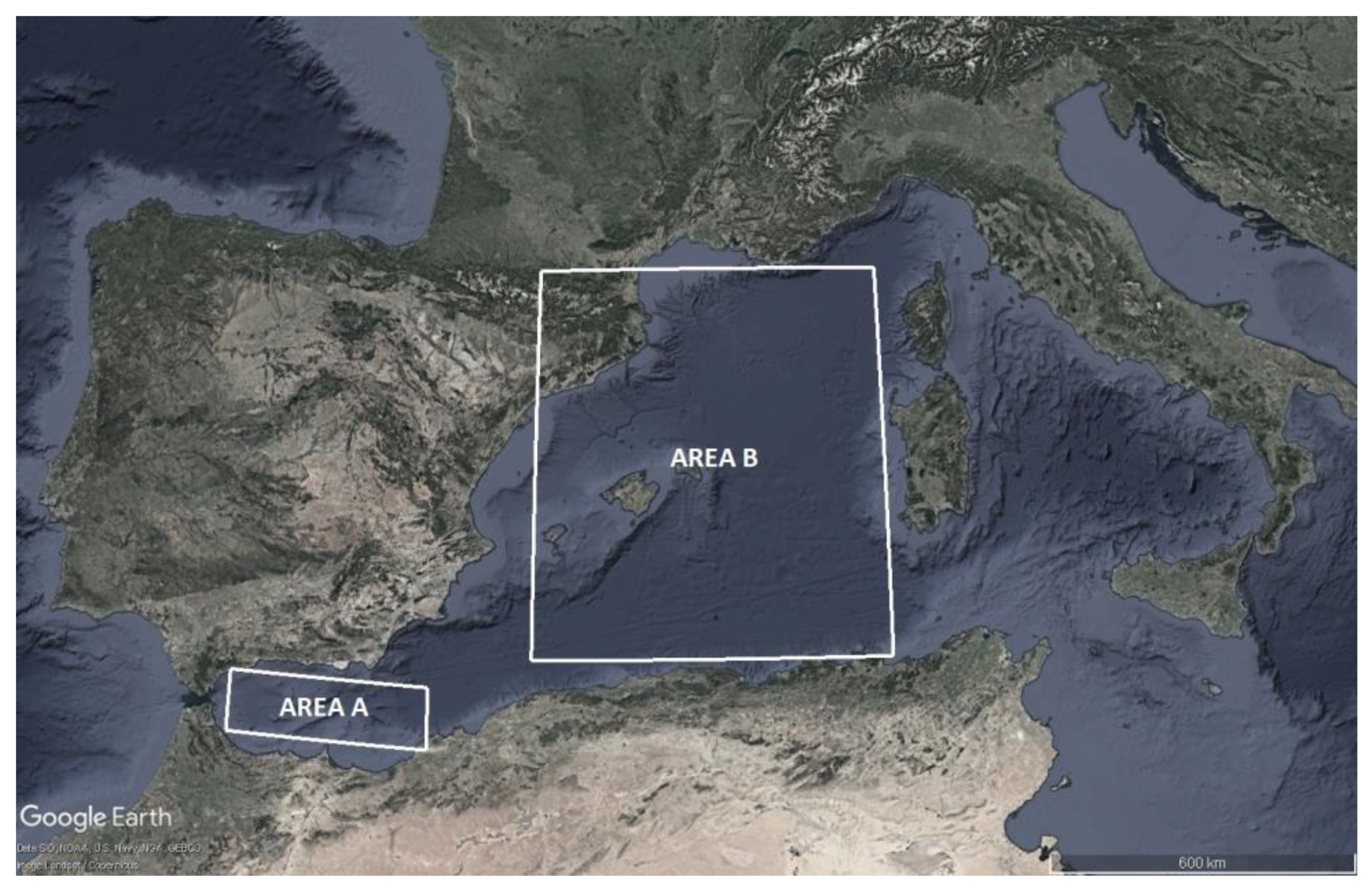
Figure 2.
Gravity anomaly data distribution in (a) AREA A and (b) AREA B.
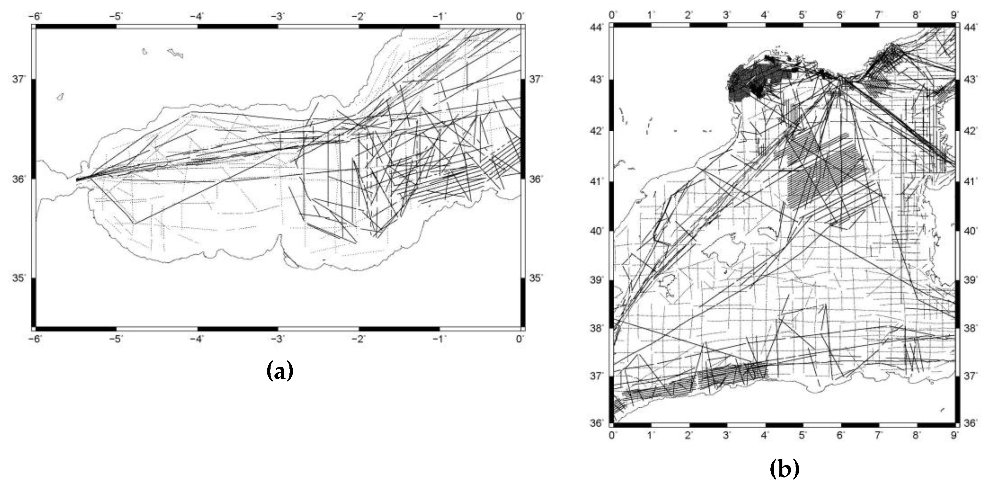
Figure 3.
Observed (a) and reduced (b) to XGM2019 gravity anomalies in AREA A.
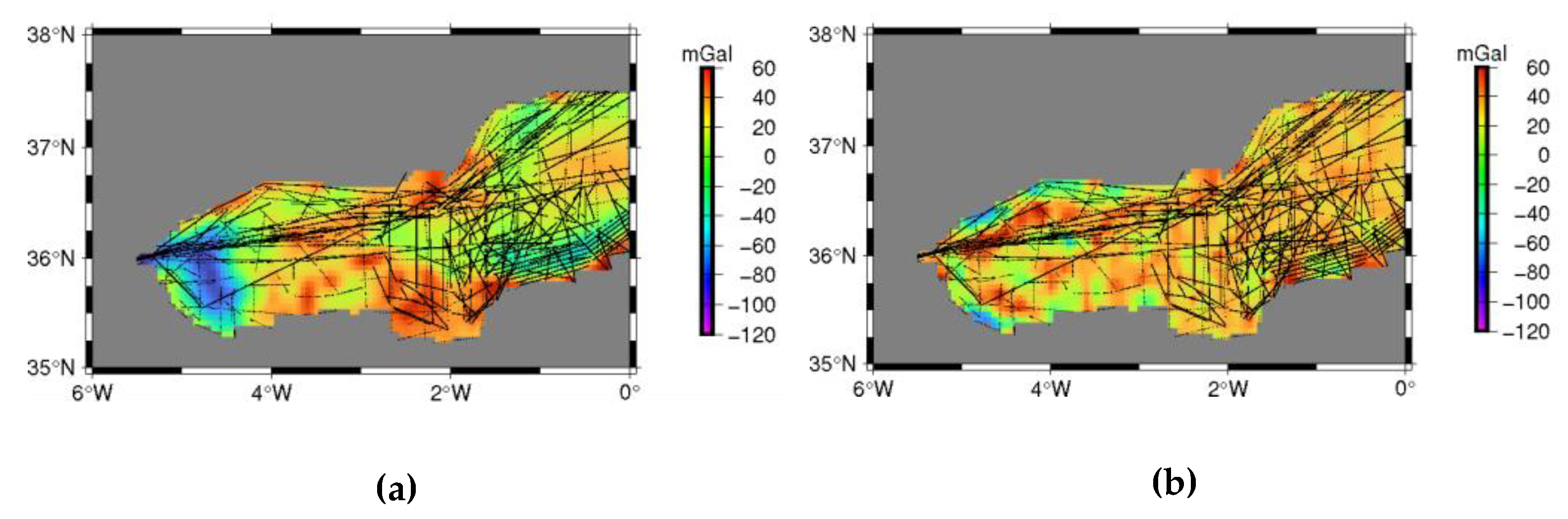
Figure 4.
Observed (a) and reduced (b) to XGM2019 gravity anomalies in AREA B.
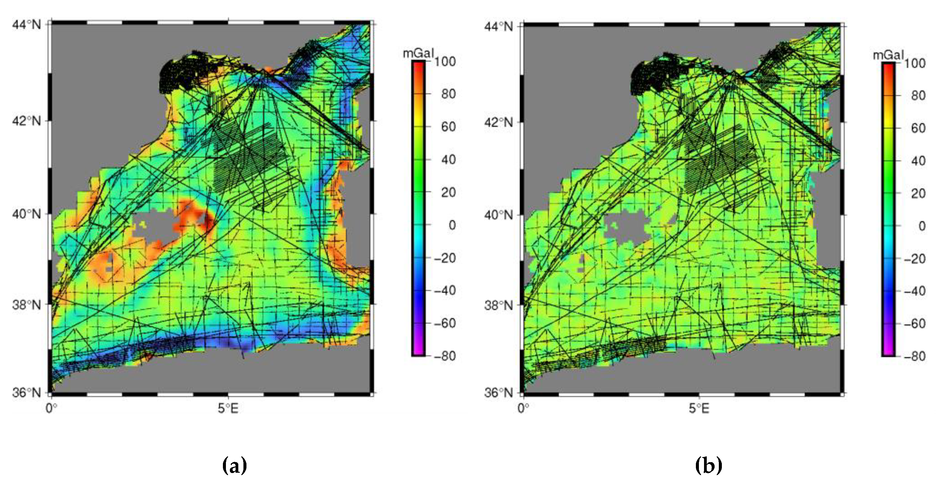
Figure 5.
Empirical covariance values (red dots) and estimated analytical model (a) exponential model, (b) planar Gaussian model, (c) ARMA model, (d) Tscherning – Rapp model in AREA A.
Figure 5.
Empirical covariance values (red dots) and estimated analytical model (a) exponential model, (b) planar Gaussian model, (c) ARMA model, (d) Tscherning – Rapp model in AREA A.
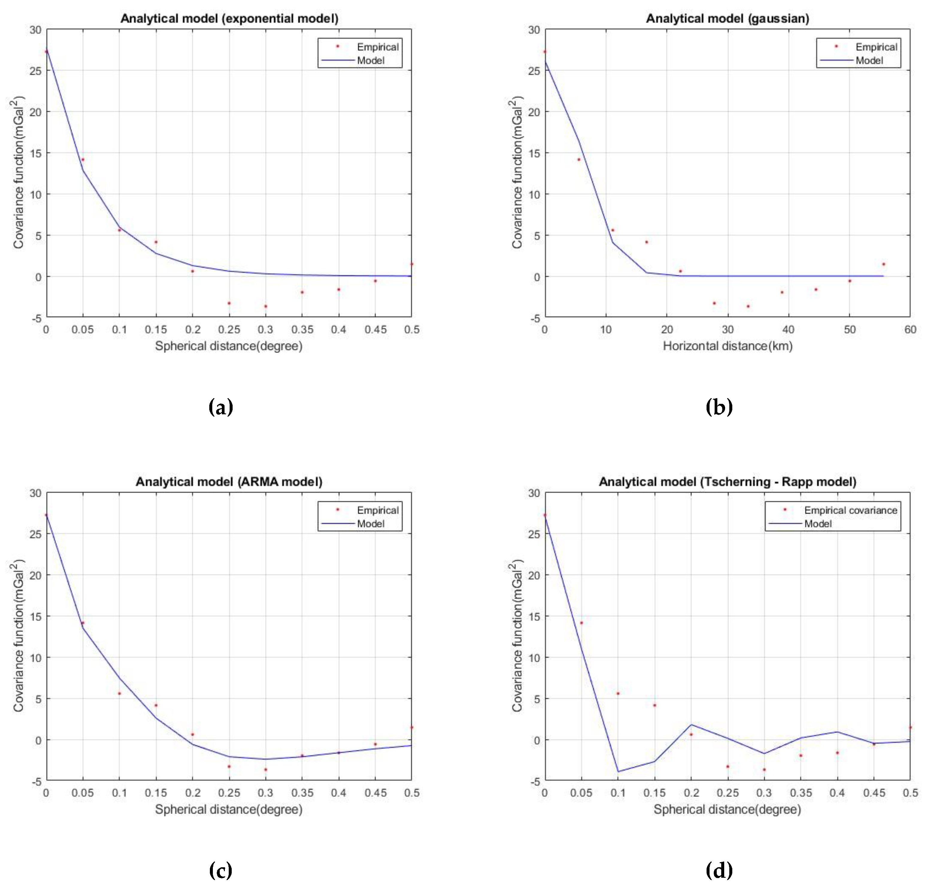
Figure 6.
Empirical covariance values (red dots) and estimated analytical model (a) exponential model, (b) planar Gaussian model, (c) ARMA model, (d) Tscherning – Rapp model in AREA B.
Figure 6.
Empirical covariance values (red dots) and estimated analytical model (a) exponential model, (b) planar Gaussian model, (c) ARMA model, (d) Tscherning – Rapp model in AREA B.
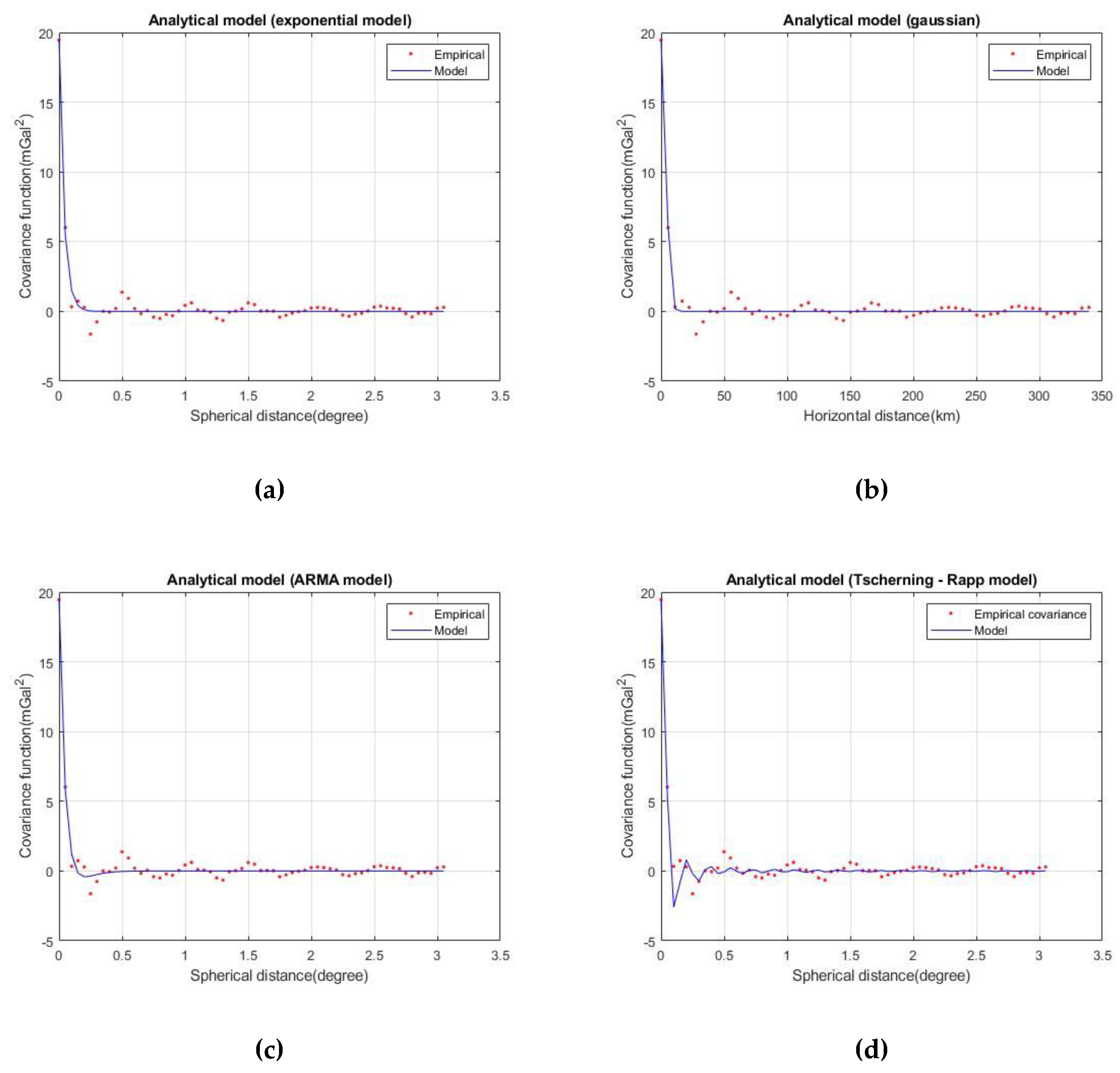
Figure 7.
The scheme of the randomly divided gravity information in (a) AREA A and (b) AREA B.
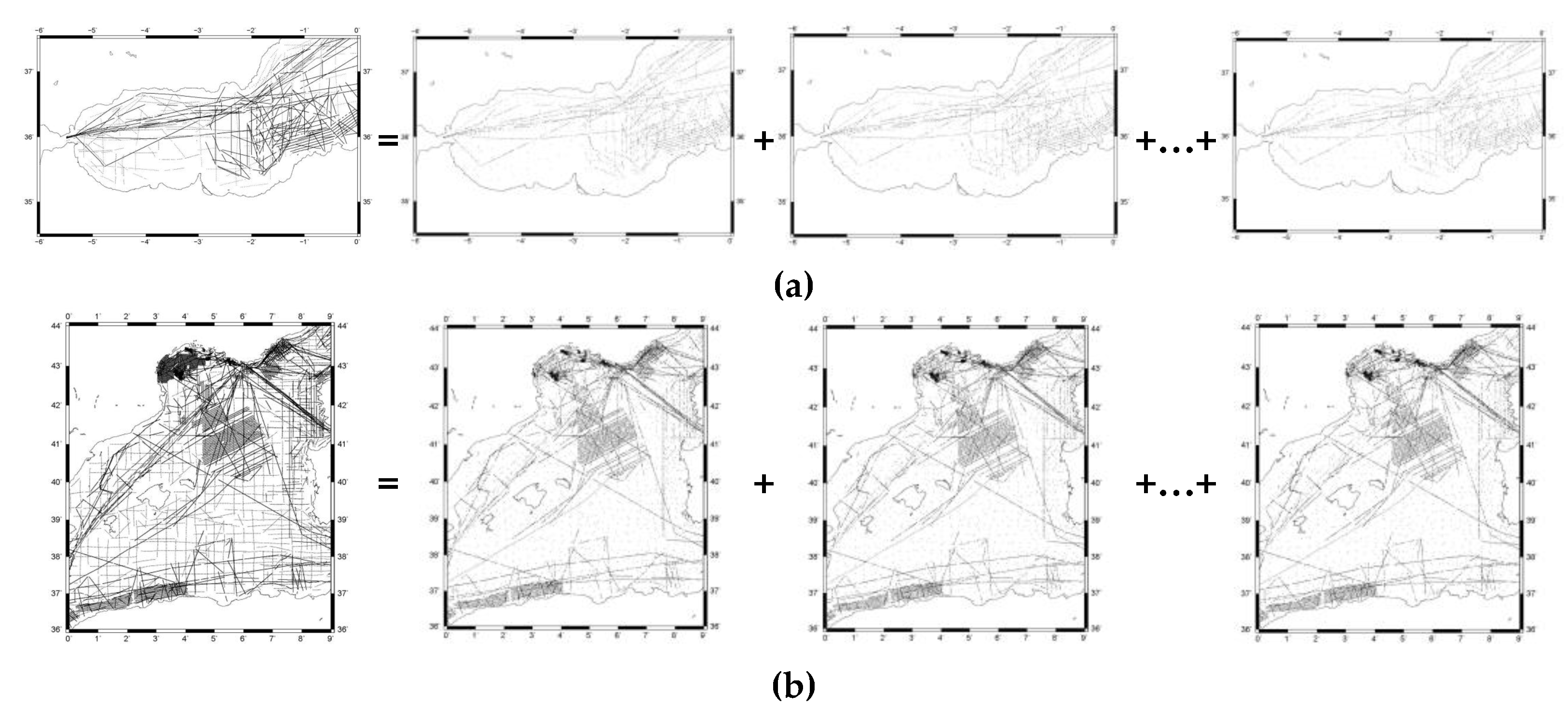
Figure 8.
The periodogram and inverse correlogram derived covariances for the gravity anomaly signal (a) and error (b) in AREA A.
Figure 8.
The periodogram and inverse correlogram derived covariances for the gravity anomaly signal (a) and error (b) in AREA A.
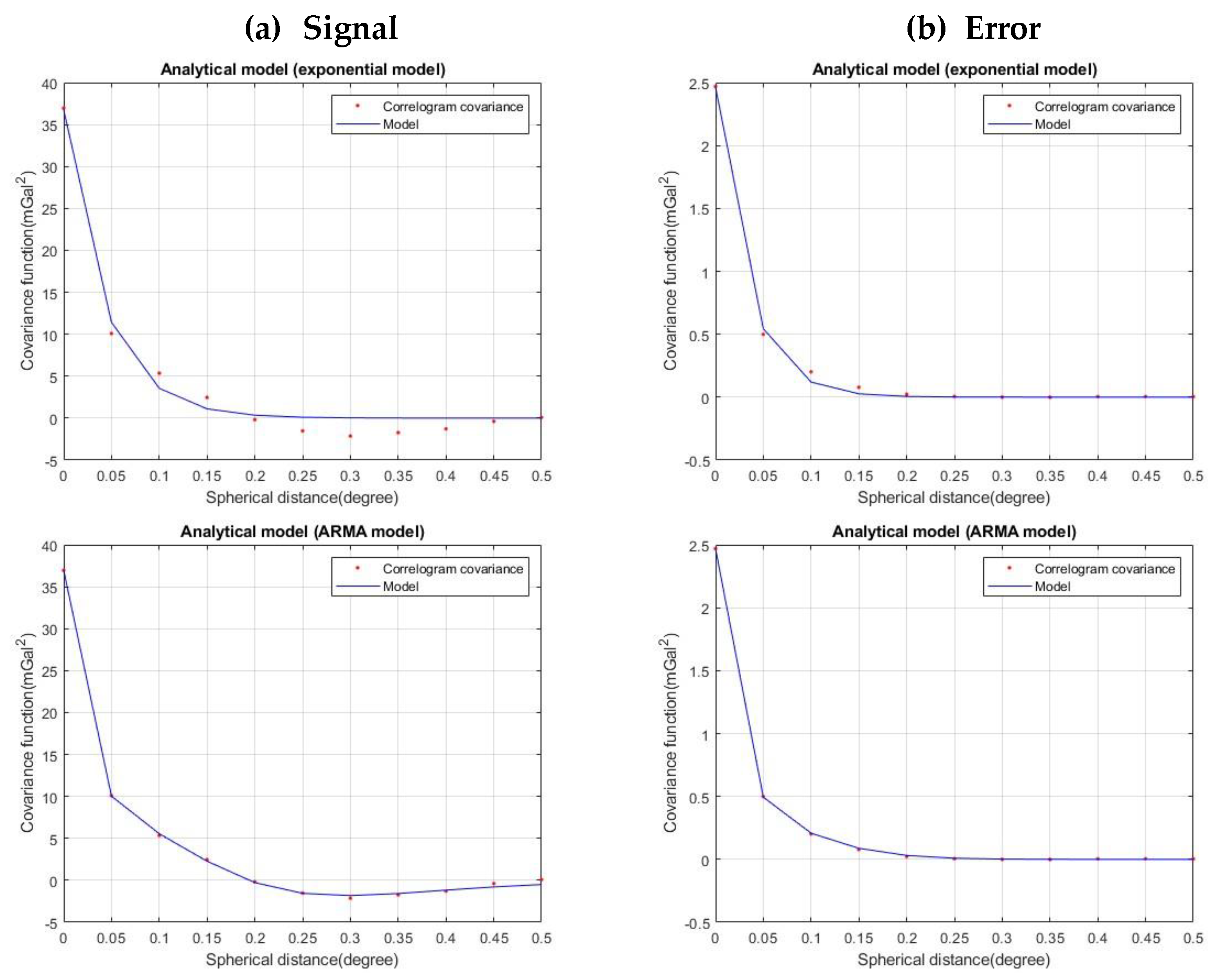
Figure 9.
The periodogram and inverse correlogram derived covariances for the gravity anomaly signal (a) and error (b) in AREA B.
Figure 9.
The periodogram and inverse correlogram derived covariances for the gravity anomaly signal (a) and error (b) in AREA B.
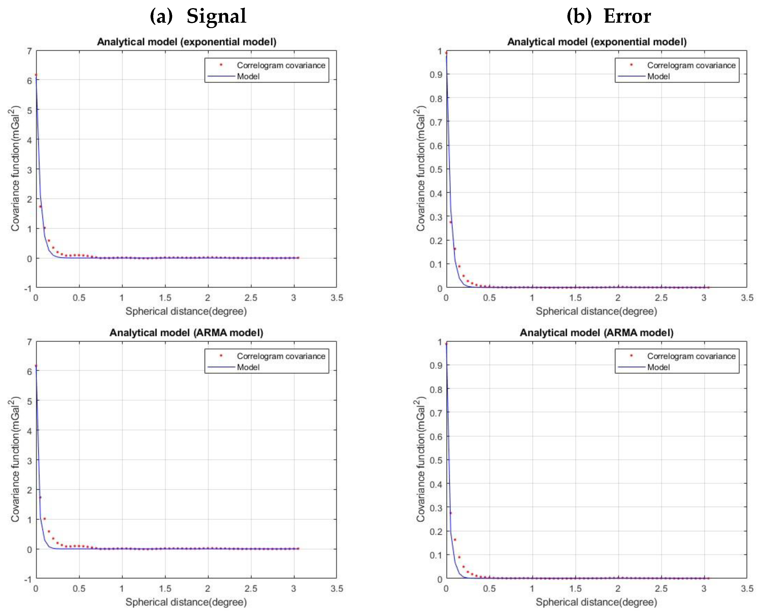
Figure 10.
The estimated signal and noise yearly altimetry covariances for 2017 in AREA A.
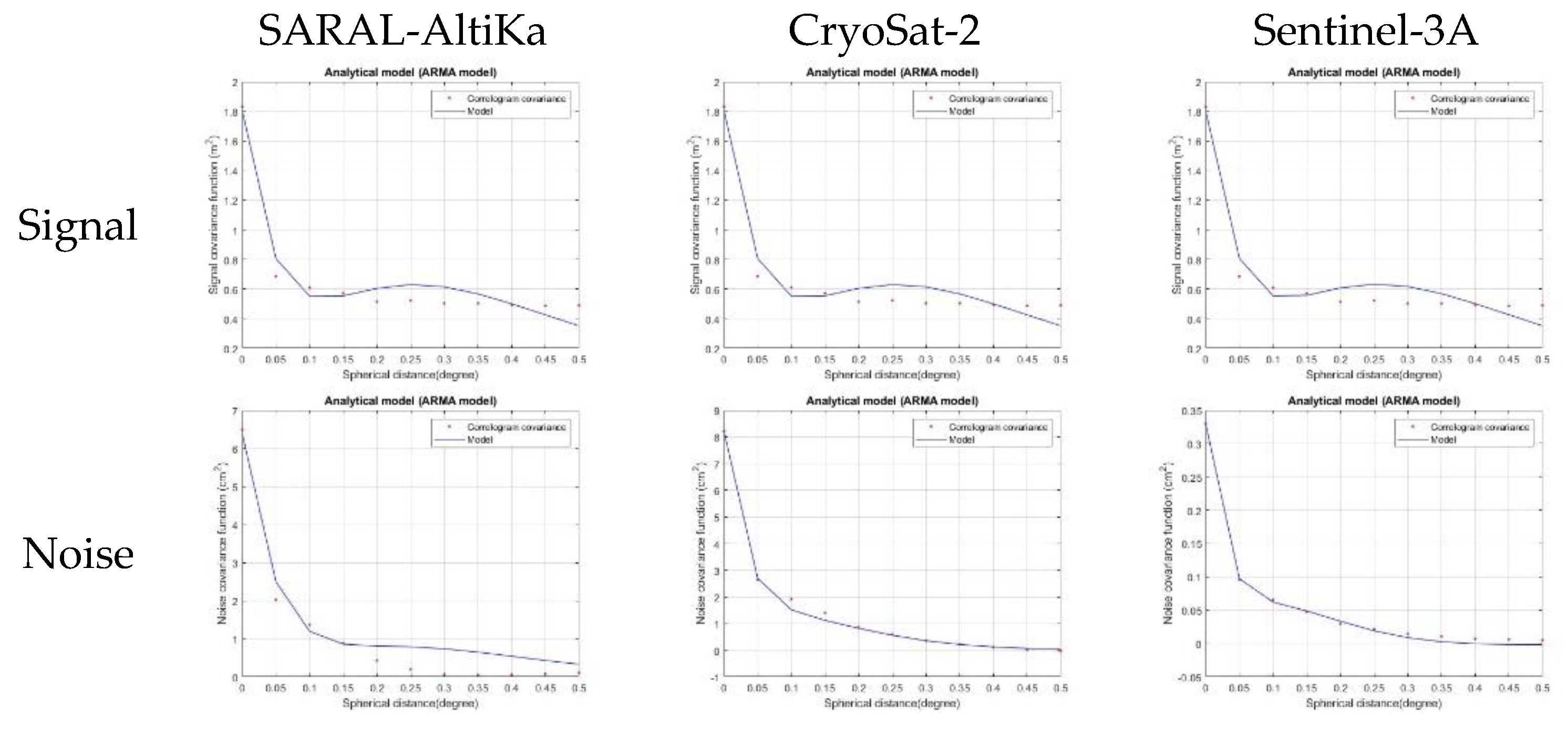
Figure 11.
The estimated signal and noise yearly altimetry covariances for the first semester of 2024 in AREA A.
Figure 11.
The estimated signal and noise yearly altimetry covariances for the first semester of 2024 in AREA A.
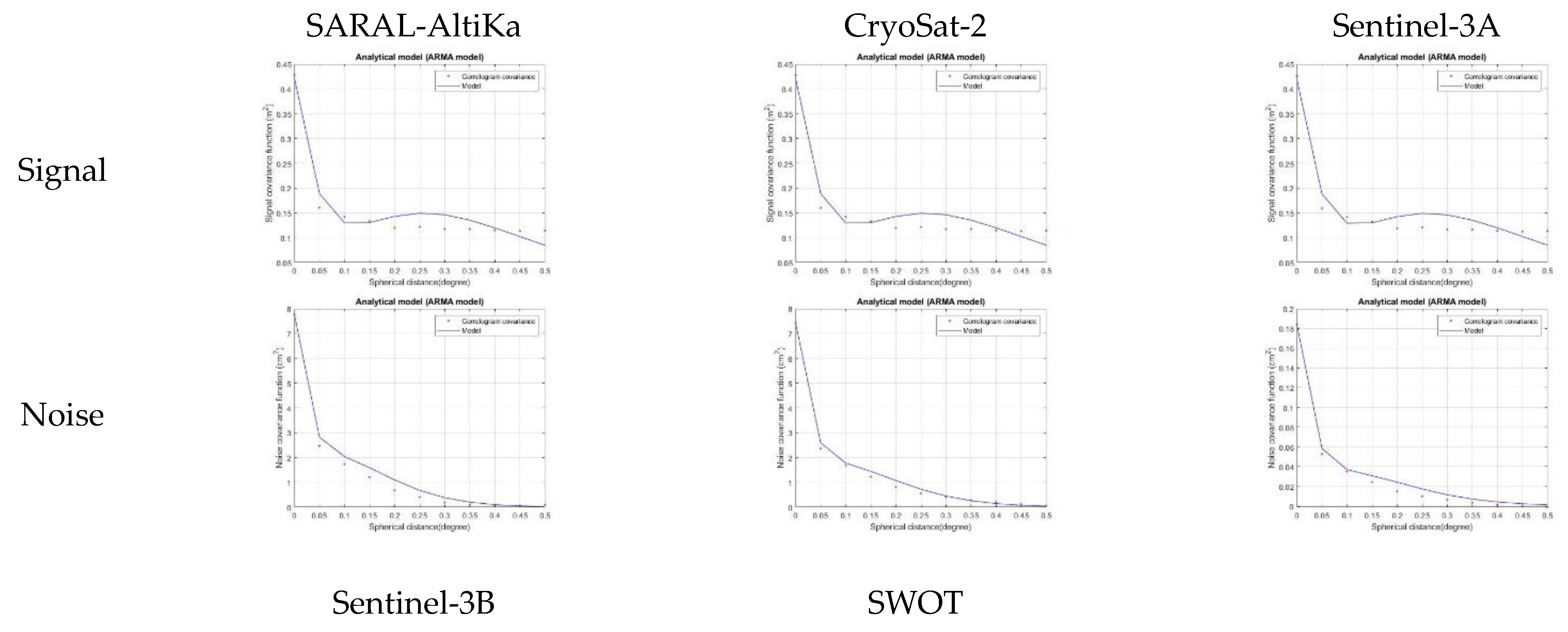
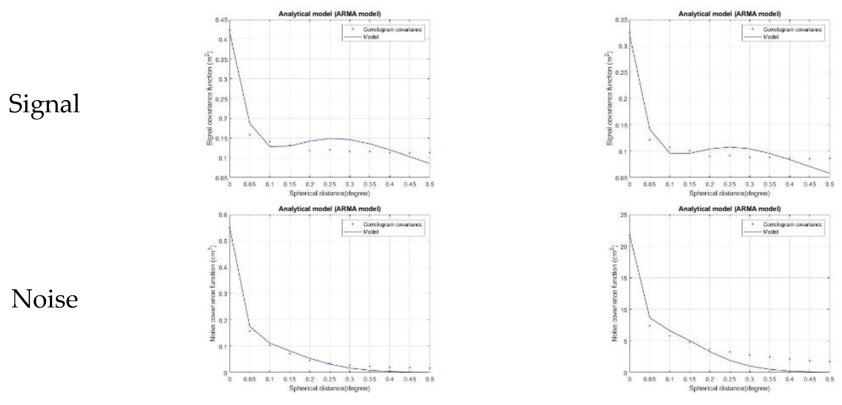
Figure 12.
The estimated signal and noise covariance for the first year of SWOT data (July 2023 – June 2024) in (a) AREA A and (b) AREA B.
Figure 12.
The estimated signal and noise covariance for the first year of SWOT data (July 2023 – June 2024) in (a) AREA A and (b) AREA B.
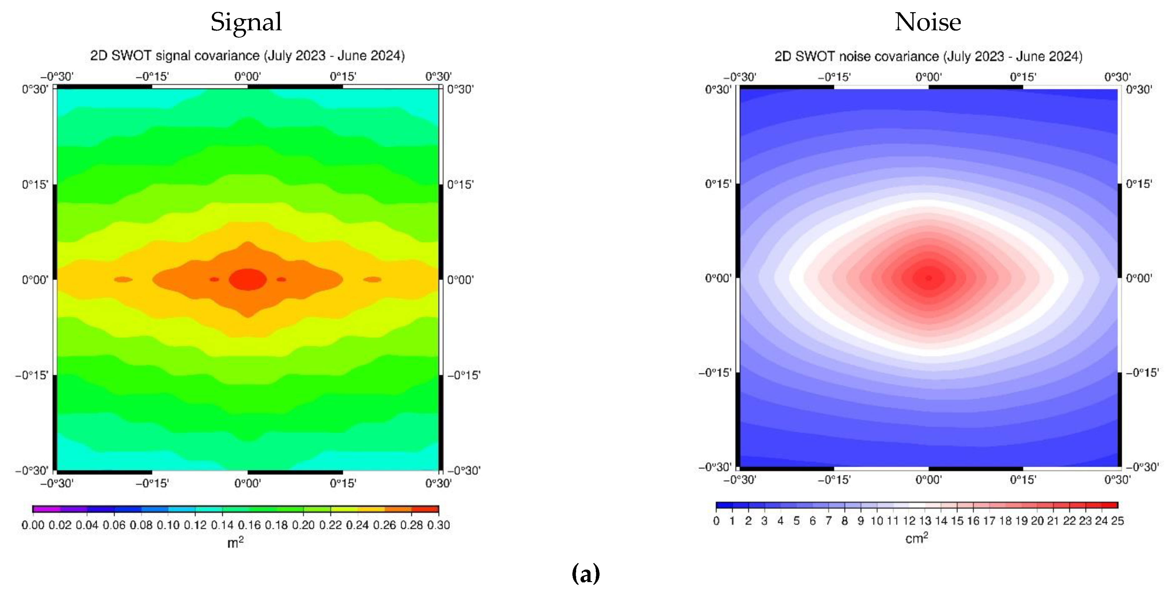
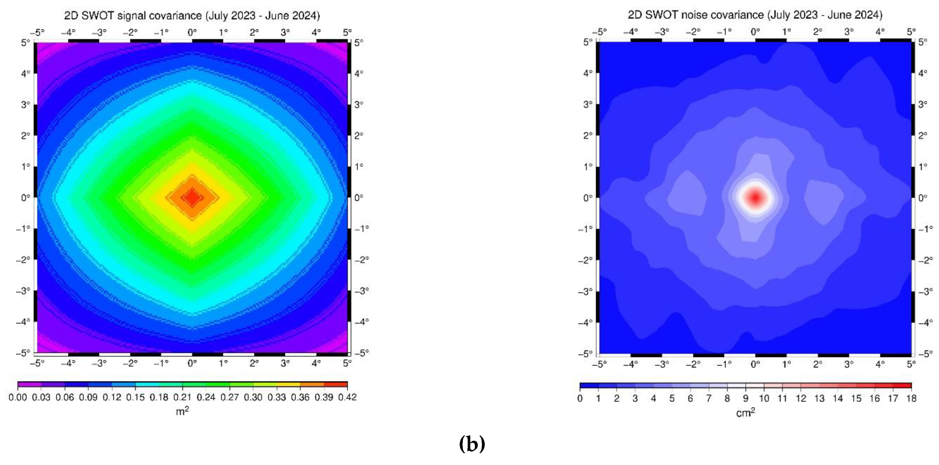
Figure 13.
MIMOS annual mean DOT estimation using real estimated gravity PSD for the year 2023 in (a) AREA A and (b) AREA B.
Figure 13.
MIMOS annual mean DOT estimation using real estimated gravity PSD for the year 2023 in (a) AREA A and (b) AREA B.
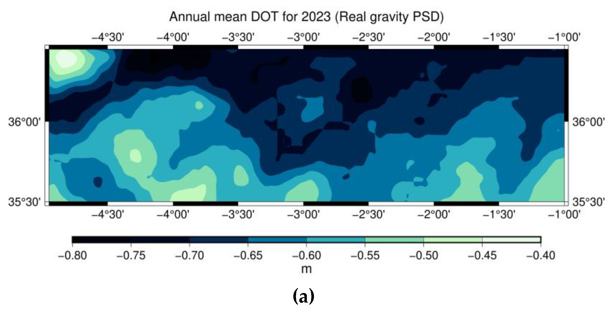
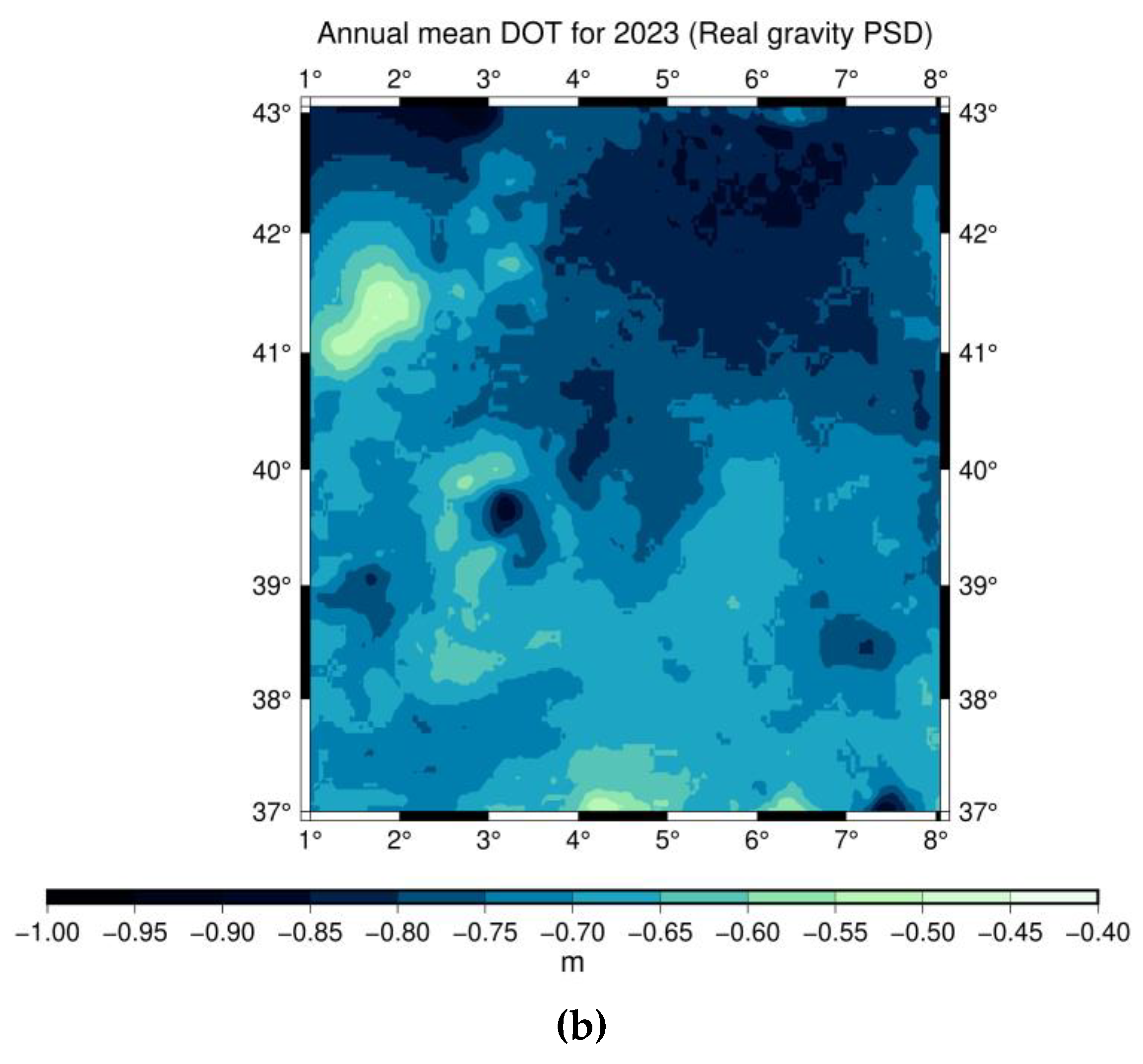
Figure 14.
Differences in the yearly mean DOT between random and estimated gravity noise solutions in AREA A for (a) year 2017 and (b) year 2024.
Figure 14.
Differences in the yearly mean DOT between random and estimated gravity noise solutions in AREA A for (a) year 2017 and (b) year 2024.
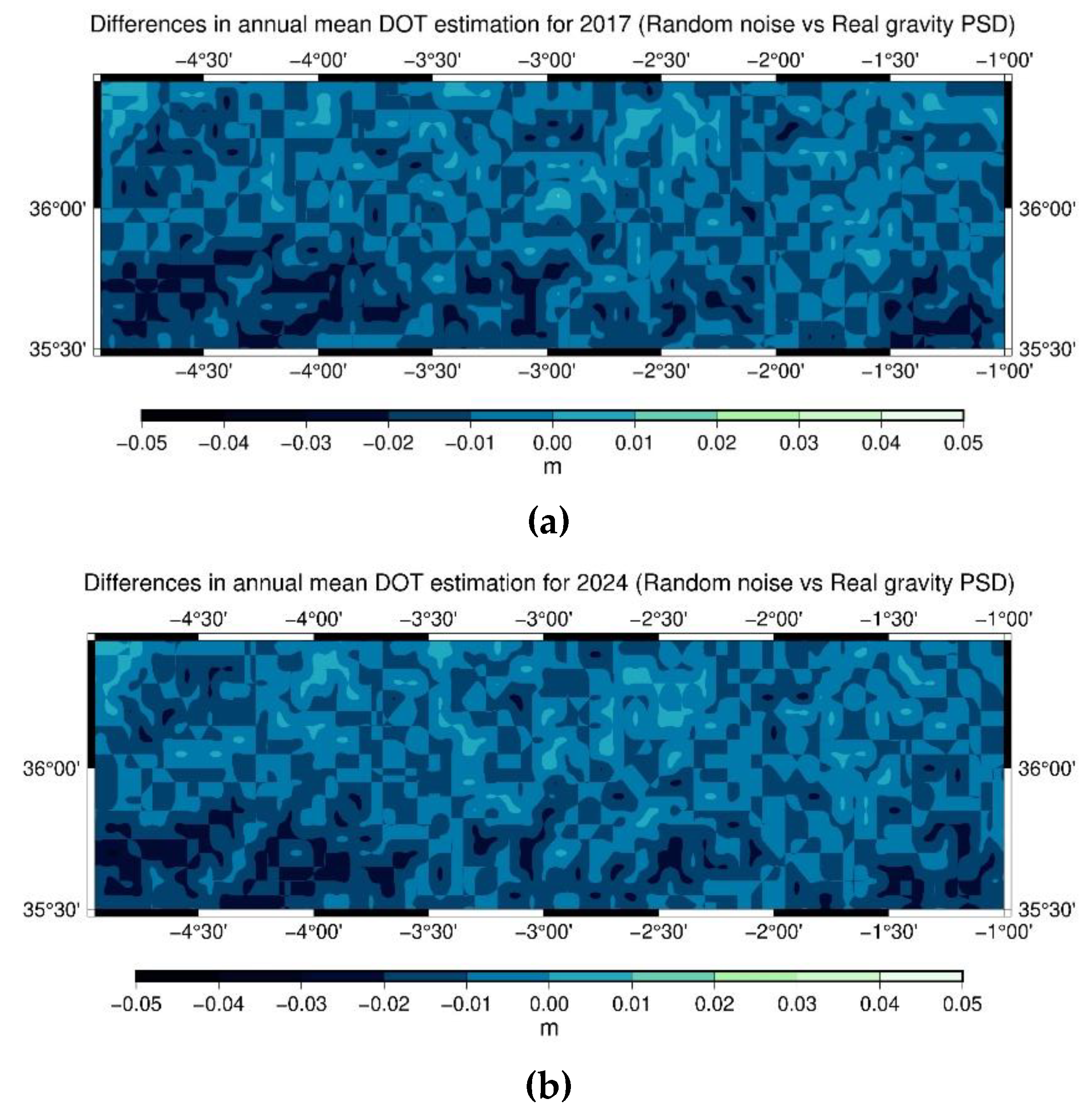
Figure 15.
Differences in the yearly mean DOT between random and estimated gravity noise solutions in AREA B for (a) year 2017 and (b) year 2024.
Figure 15.
Differences in the yearly mean DOT between random and estimated gravity noise solutions in AREA B for (a) year 2017 and (b) year 2024.
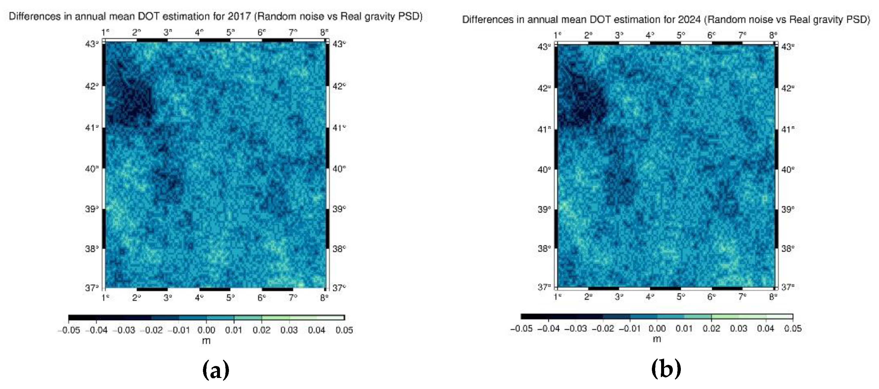
Figure 16.
Estimated 2D and averaged 1D mean DOT output error covariances for the year 2017 in AREA A (a) using simulated noise and (b) estimated PSD for the gravity data.
Figure 16.
Estimated 2D and averaged 1D mean DOT output error covariances for the year 2017 in AREA A (a) using simulated noise and (b) estimated PSD for the gravity data.
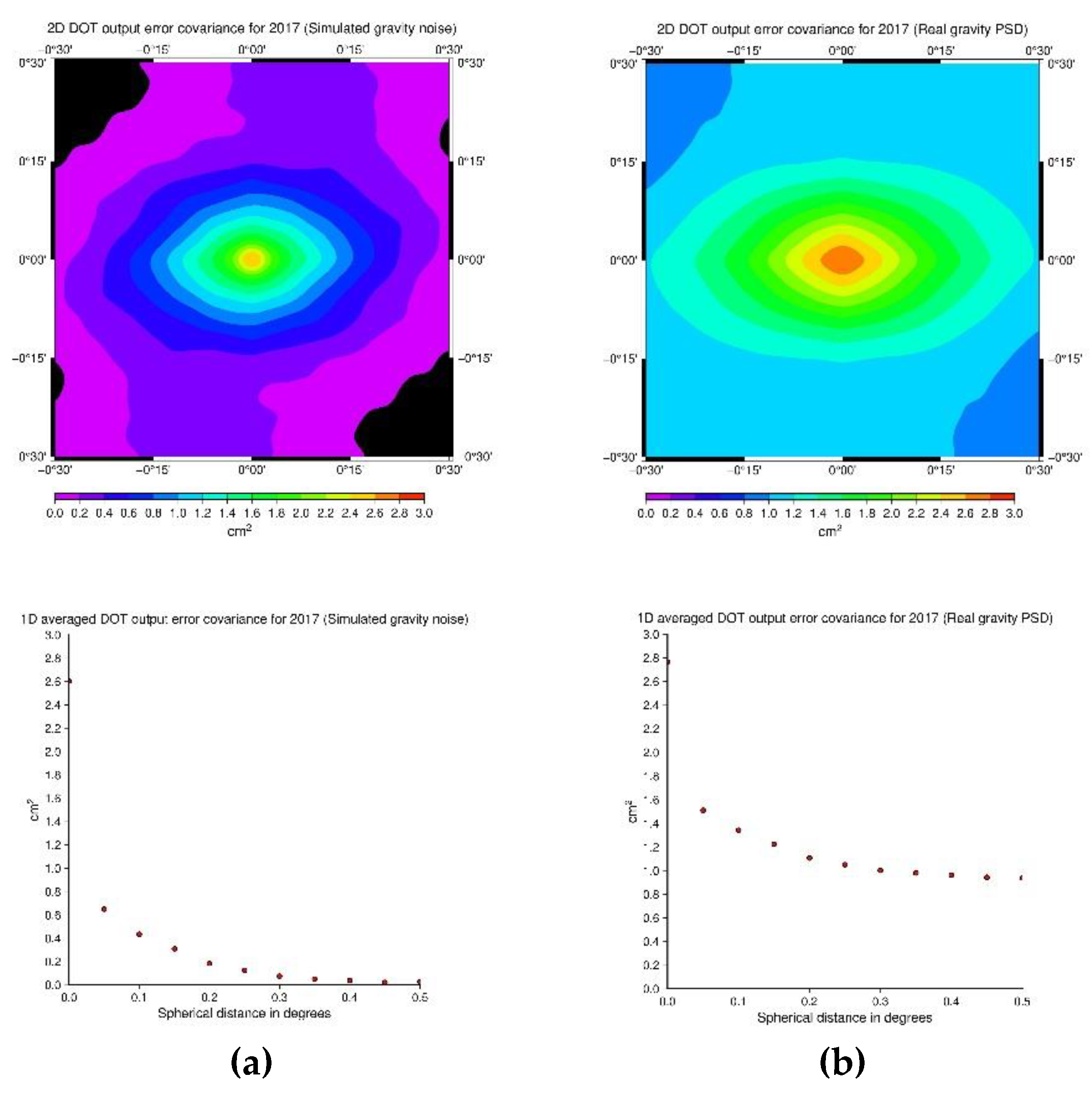
Figure 17.
Estimated 2D and averaged 1D mean DOT output error covariances for the year 2023 in AREA B (a) using simulated noise and (b) estimated PSD for the gravity data.
Figure 17.
Estimated 2D and averaged 1D mean DOT output error covariances for the year 2023 in AREA B (a) using simulated noise and (b) estimated PSD for the gravity data.
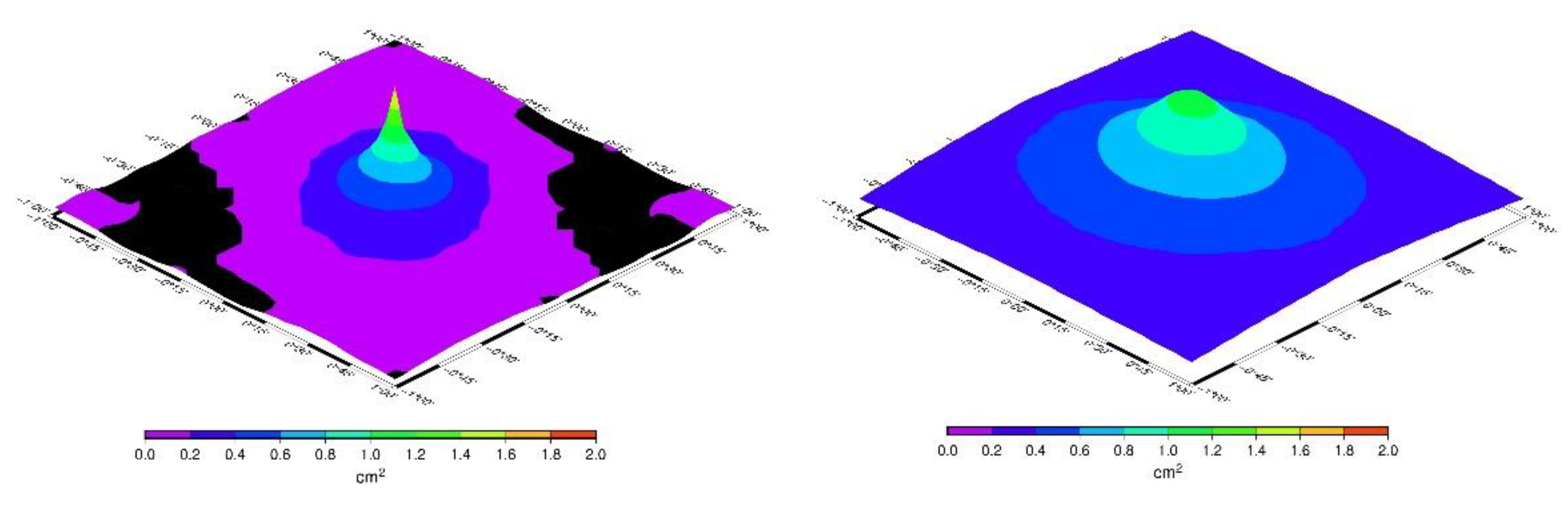
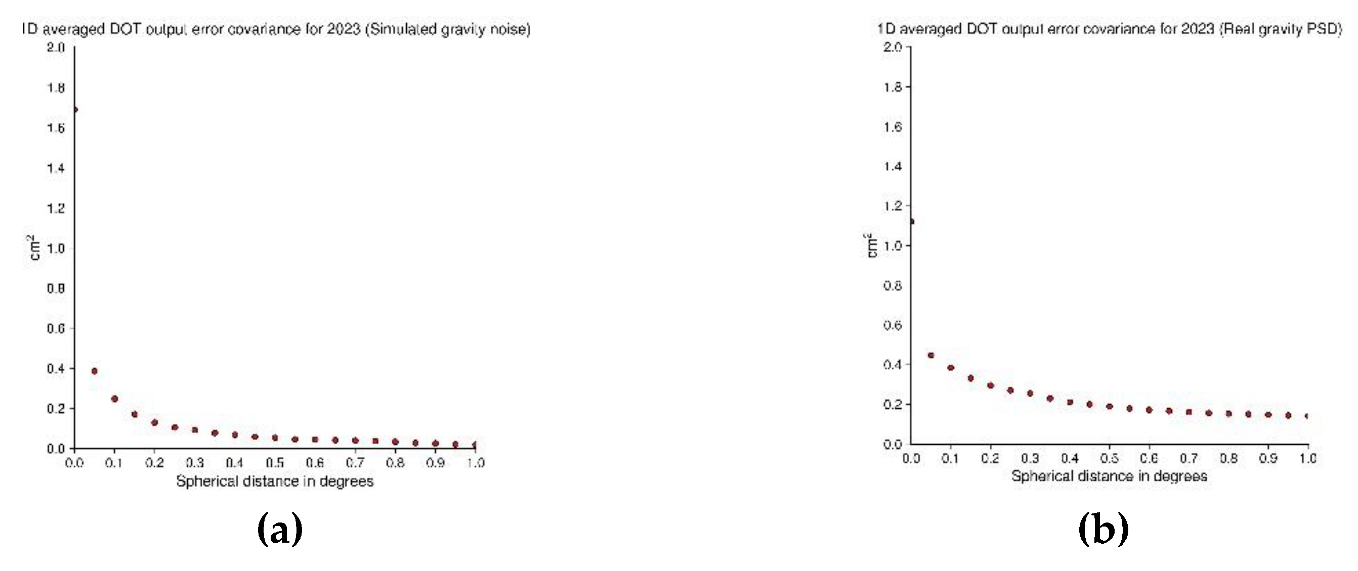

Table 1.
The statistics of the reduced gravity anomalies in AREA A (all values in mGal).
| max | min | mean | sd | rms | |
| Δg (obs) | 70.699 | -131.949 | -23.758 | 39.820 | 31.956 |
| Δg (red) | 26.888 | -46.216 | 0.278 | 5.776 | 5.769 |
Table 2.
The statistics of the reduced gravity anomalies in AREA B (all values in mGal).
| max | min | mean | sd | rms | |
| Δg (obs) | 98.243 | -80.085 | -7.168 | 25.727 | 24.708 |
| Δg (red) | 42.696 | -33.438 | -0.225 | 4.612 | 4.606 |
Table 3.
Results of the analytical model validations – AREA A.
| model | σ2 (mGal2) | misfitcoef | corrcoef |
| Simple exp. | 4.982 | 0.926 | 0.983 |
| Gaussian | 6.238 | 0.917 | 0.968 |
| ARMA | 2.620 | 0.955 | 0.991 |
| Tscherning - Rapp | - | 0.851 | 0.900 |
Table 4.
The results of the analytical model validations – AREA B.
| model | σ2 (mGal2) | misfitcoef | corrcoef |
| Simple exp. | 0.200 | 0.977 | 0.985 |
| Gaussian | 0.178 | 0.979 | 0.987 |
| ARMA | 0.192 | 0.978 | 0.987 |
| Tscherning - Rapp | - | 0.970 | 0.975 |
Table 5.
Results of the analytical model validations – AREA A.
| Signal | Error | |||
| model | σ2 (mGal2) | corrcoef | σ2 (mGal2) | corrcoef |
| Simple exp. | 2.156 | 0.994 | 0.001 | 0.999 |
| ARMA | 0.120 | 0.999 | 0.000 | 0.999 |
Table 6.
Results of the analytical model validations – AREA B.
| Signal | Error | |||
| model | σ2 (mGal2) | corrcoef | σ2 (mGal2) | corrcoef |
| Simple exp. | 0.083 | 0.994 | 0.000 | 0.995 |
| ARMA | 0.000 | 0.984 | 0.000 | 0.990 |
Disclaimer/Publisher’s Note: The statements, opinions and data contained in all publications are solely those of the individual author(s) and contributor(s) and not of MDPI and/or the editor(s). MDPI and/or the editor(s) disclaim responsibility for any injury to people or property resulting from any ideas, methods, instructions or products referred to in the content. |
© 2025 by the authors. Licensee MDPI, Basel, Switzerland. This article is an open access article distributed under the terms and conditions of the Creative Commons Attribution (CC BY) license (http://creativecommons.org/licenses/by/4.0/).
Copyright: This open access article is published under a Creative Commons CC BY 4.0 license, which permit the free download, distribution, and reuse, provided that the author and preprint are cited in any reuse.


