Submitted:
05 August 2025
Posted:
06 August 2025
You are already at the latest version
Abstract
In early 2025, the Jason-3 satellite orbit was maneuvered from the "interleaved" orbit to a tandem configuration with the Sentinel-6A satellite, concurrent with the upgrade of its Geophysical Data Records (GDR) from Version F to G. To date, six complete cycles of GDR-G products have been released, featuring notable improvements such as the official replacement of the MLE3 retracker with the Adaptive retracker for Sea Surface Height Anomaly (SSHA) calculations. This study aims to evaluate GDR-G performance by analyzing SSHA under eight error correction strategies, using the last six GDR-F cycles and first six GDR-G cycles. Key findings include: significantly reduced SSHA noise in GDR-G compared to GDR-F; relative biases of up to ~4 cm in sea surface height when using different retracking algorithms or correction strategies; and optimal accuracy achieved with the Adaptive retracker combined with 3D sea state bias (SSB) correction. Comparative analysis of Significant Wave Height (SWH), backscattering coefficient (Sigma-0), and wind speed (WS) between MLE4 and Adaptive retrackers revealed anomalies in Adaptive results: clustered SWH outliers near 0 m and 4 m, and WS outliers slightly above 28 m/s. These anomalies, linked to invalid MLE4 retracking results and non-Brownian echo shapes (coastal/inland waters, sea ice), suggest that refining the Adaptive retracker or developing new algorithms could further enhance Jason-3’s observational performance.
Keywords:
satellite altimetry
; Jason-3
; geophysical data records
; sea surface height anomaly
; retracker
; significant wave height
; wind speed
1. Introduction
Since the launch of Topex / Poseidon satellite in 1992, satellite altimetry has been one of the indispensable data sources in oceanography and marine geodesy community [1]. TOPEX/Poseidon satellite and its successors (Jason-1, Jason-2, Jason-3, Sentinel-6A satellites, all these satellites are usually called “Jason-series” missions) has routinely provided global sea surface height, significant wave height and sea surface wind speed measurements for over three decades. The data provided very clear evidences of the global sea level rise [2,3].
The Jason-series missions are defined as the “reference missions” in the altimetry community. In the early life of a new Jason-series satellite, it is crucial to make sure that the measurements are stable and consistent, so the satellite usually operated in the “tandem phase” in which the new satellite (e.g., Sentinel-6A) and its precursor (e.g., Jason-3) share the same ground track within a very short time lag. Relative calibration based on the tandem configuration has significant advantage over crossover calibration: more valid measurement-pairs can be compared, and most errors in the SSHA (Sea Surface Height Anomaly; some researchers may be more familiar with its alias: SLA (Sea Level Anomaly)) computation can be canceled out.
In the past, there was only one tandem phase between successive missions. But the Jason-3 / Sentinel-6A tandem mission has brought many benefits, and a second tandem mission was strongly recommended [4]. The Jason-3 orbit was maneuvered in January 2025, returning to its initial orbit (same track with the Sentinel-6A). Meanwhile, its data (Geophysical Data Records, GDR) was upgraded to the new version labelled “G” [5]. Therefore, it is necessary to conduct an assessment of the performance of GDR-G data as soon as possible.
2. The evolution of Jason-3 GDR Standards
For the modern altimetry missions, the data processing methodology and the auxiliary data source keep evolving, and the GDR data standards upgrade accordingly. In the early mission of Jason-3 (since September 2016, the end of its Cal/Val phase), the GDR obeyed the “GDR-D” standard, and GDR-F was introduced in September 2020 [6]. GDR-F was a significant improvement over GDR-D: the parameters were arranged as groups; the reference ellipsoid was changed to WGS84 instead of Topex / Poseidon [7] (there were biases of ~70 centimeters between the two ellipsoids!), a number of auxiliary models to calculate the error items were upgraded, and more important, an innovative retracker called “Adaptive Retracker” was introduced [8,9,10].
For more than one decade, the official GDR products of Jason missions had two operational retrackers: MLE3 and MLE4 [11]. In these two retrackers, the waveforms were fitted to the Brown [12] or Hayne [13] model, the radar altimeter Point Target Response (PTR) in the retracker was approximated to Gaussian shape to improve the computation efficiency, and the MLE was realized by (weighted) least square criteria. The only difference between MLE3 and MLE4 was the estimation of the satellite off-nadir angle: in MLE3, the satellite off-nadir angle was estimated from the trailing-edge slope of the logarithmic power spectrum; while in MLE4, the satellite off-nadir angle was a parameter in the least square procedure. The Adaptive retracker is a three-discipline improvement over MLE3 and MLE4:
- A new waveform model (the Adaptive model) replaces the Brown or Hayne model, adding a parameter correlated to the mean square slope (describing the sea surface roughness) of the reflective surface, significantly improving the retracking success rate for peaky waveforms.
- Real radar PTR is numerically convolved with the two other terms (the flat sea surface response and the sea surface elevation pdf) in the analytical model of waveform.
- A true MLE approach (using the exact likelihood function) is used that accounts for the statistics of the speckle noise presented in the echo waveforms.
The GDR-G standard roughly aligns with the GDR-F standard. Maybe the most important improvement is replacing MLE3 retracker parameters by adaptive retracker parameters (particularly “ssha_adaptive”). The parameters based on MLE4 retracker is still the default parameter. MLE3 range measurements are still provided, but the SSHA cannot be calculated because of the lack of proper correction terms dedicated to MLE3 retracker. Another improvement worthy to mention is the ionospheric correction, the Dettmering [14] algorithm was adopted. As for the wet tropospheric correction, the Jason-3 AMR (Advanced Microwave Radiometer) drift was also detected and corrected. Several models were also upgraded [5], as tabulated in Table 1.
The Jason-3 satellite GDR-G data have been released only a few months, and there is little research published on the evaluation of this dataset. To fully exploit the potential of the data, it is necessary to know the main characteristics of the data, such as the potential bias and the precision when different error source was adopted. In this article, we attempted to conduct intensive analysis of the data, focusing on the SSHA under different retracker and different error correction source. Besides, SWH (Significant Wave Height), Sigma-0 (backscattering characteristics) and WS (Wind Speed) were also analyzed and several interesting features were found.
3. Data and Methods
3.1. Data
The release of Jason-3 GDR-G was coincident with the maneuver of satellite to form a tandem configuration the with Sentinel-6A satellite. In the half of Cycle #400, the satellite orbit was maneuvered to the second tandem phase the with Sentinel-6A satellite, and the cycle labels were reassigned (beginning with #500) in the new phase. Therefore, Cycle #501 is the first cycle which has complete GDR-G data product. Up to July 2025, GDR-G of only six cycles (Cycle #501~#506, spanning from 06/11/2024 to 02/01/2025) has been disseminated. These data were the primary data source of this work. As the counterpart of GDR-G, the last six cycles of GRD-F (Cycle #394~#399, spanning from 01/02/2025 to 02/04/2025) were also collected to conduct a comparative analysis. Therefore, twelve cycles of Jason GDR data were considered in this work.
3.2. Methods
3.2.1. Computation of SSHA
The primary objective of an altimetry mission is to measure the SSH (Sea Surface Height) and SSHA. SSH is the height of the sea surface above the reference ellipsoid. It can be calculated as following:
where H is the orbital height, R is the range from the satellite to the sea surface (measured from the altimeter, and the instrumental errors have been compensated), , and are the three components of the atmospheric path delay (dry tropospheric delay, wet tropospheric delay and ionospheric delay, respectively). , is the sea state bias.
SSHA is defined here as the SSH minus the mean sea surface and minus known geophysical effects [8]:
where MSS is the Mean Sea Surface, geocentric ocean tide height (including ocean load tide height), is the solid earth tide height, is the pole tide height, (based on the work of Zaron [15], and introduced in GDR-F), is the non-equilibrium long period tide height, is the dynamic atmospheric correction (the summation of inverse barometric correction and high frequency fluctuations correction).
For several correction items, Jason-3 GDR provides two solutions. The solutions used in the computation of the official “ssha” parameters are defined as the “baseline solution”, and SSHA can also be calculated if we replace any baseline solution by the corresponding secondary solution.
SSHAs of eight retracking / error correction strategies were calculated (if possible) for every 1Hz measurement point of Jason-3 altimeter:
- Baseline (MLE4): directly extracted from the data products (all the corrections was same to the “baseline solution” column of Table 2).
- 3D SSB (MLE4): same to Strategy 1, except that the 2D (two dimensions, SWH + WS) sea state bias correction was replaced by its 3D (three dimensions, SWH + WS + mean wave period) counterpart.
- Model wet tropospheric (MLE4): same to Strategy 1, except that the microwave radiometer-derived wet tropospheric delay correction was replaced by a model (ECMWF) solution.
- GIM ionospheric (MLE4): same to Strategy 1, except that the dual-frequency altimeter-derived ionospheric delay correction was replaced by a model (GIM) solution.
- GOT tide (MLE4): same to Strategy 1, except that the LEGOS FES model-derived ocean tide height was replaced by another model (NASA GOT) solution.
- DTU MSS (MLE4): same to Strategy 1, except that the CNES_CLS (for GDR-F) or Hybrid (for GDR-G) MSS was replaced by another model (DTU) solution.
- Baseline (Adaptive): For GDR-G, directly extracted from the data products (all the corrections was same to the “baseline solution” column of Table 2); for GDR-F, calculated from.
- 3D SSB (Adaptive) same to Strategy 1, except that the 2D (SWH + WS) sea state bias correction was replaced by its 3D (SWH + WS + mean wave period) counterpart.
Improvement of 3dSSB (Adaptive) over Baseline (MLE4)
The radar altimeter range measurements were retrieved based on the retracking of the radar echo waveforms, so different retracker can lead to different SSHA. Two baseline SSHAs are provided both in GDR-F (MLE4 and MLE3) and GDR-G (MLE4 and Adaptive). Aside from the range, the ionospheric path delay and sea state bias corrections are also dependent on particular retracker. In GDR-G, both the ionospheric path delay and sea state bias corrections of MLE3 retracker are no longer provided, making it impossible to calculate the suitable SSHA. Fortunately, the ionospheric path delay and sea state bias corrections of Adaptive retracker were included in GDR-F, so it is possible to calculate the Adaptive SSHA for GDR-F from Eq. (1) and (2).
After computing the SSHAs, we carried out a simple editing of the data. Firstly, the robustness of the MLE retracker (only ~70% success rate) was much worse than the Adaptive retracker (~90% success rate). Therefore, only those measurements which had both MLE4 and Adaptive SSHAs were considered in the comparative analysis to eliminate the representative errors. Secondly, the SSHA measurements with an absolute value of 1 meter are also rejected as outliers. In fact, aside from the severe situation such as storm surge or heavy rain events, the actual SSHA was usually within ±0.2 meters. For all the cycles, more than 500,000 valid measurements were included in the analysis, guaranteeing the statistical significance.
3.2.2. Evaluation of the SSHA noise level
After acquiring several SSHA from the same dataset, one natural question is to compare them and, hopefully, get figures that can quantitively evaluate the contribution (or).
There are several methods to evaluate the SSHA noise level. One is based on the power level of white-noise region of the power spectrum of SSHA time series. The spectrum is acquired using the FFT (Fast Fourier Transform) technique, so it is necessary to find enough long continuous SSHA time series (if there were gap points, interpolation may bring errors). In only two months the number of suitable time series is limited, and the intersection of linear-decreasing region and white-noise region may be ambiguous. Another popular approach is the self-cross calibration between ascend and descend passes, there are time lag between the ascend and descend passes at crossover points, leading to mismatch errors.
In this article, we propose a “detrend method”. The idea is to filter out the trend of the SSHA. Unlike the geoid, the SSHA would unlike to change significantly in spatial dimension. We conducted a moving average of the along-track SSHA series, and removed the smooth SSHA to get the SSHA residual series:
The core consideration in this method is to set the length of moving window. The detrend procedure can be regarded as a high-pass filtering. The shorter the window, the higher cutoff of the high-pass filter, and it can be expected that some small scale or mesoscale components of the correction terms were also filtered out. Although the standard deviation of the SSHA residual series would be lower, the standard deviation of different strategies would be very similar (e. g., if we use a 21-point moving average, we can hardly discern the difference of the SSHA series between Strategy 1 and Strategy 3). As a good compromise, we choose 61-point (equivalent to the scale of ~350 km, given a ~ 5.8 km/s satellite ground speed) boxcar moving average in all the processing. Some actual SSHA signal (such as mesoscale eddies) would be aliased in the residual series (which should be pure errors in ideal case), but most error signals (atmospheric path delay, SSB, tides, etc.) would retain, facilizing further analysis.
3.2.2. The SWH, Sigma-0 and WS Analyzing Method
SWH, Sigma-0 and WS, sometimes called “wind-and-wave” products, are very important parameters in dynamic oceanography. More importantly, SSB, whose accuracy is dependent on the SWH and WS, has become the leading error source in SSHA, highlighting the necessity of the evaluation of “wind-and-wave” products.
In the SWH, Sigma-0 and WS analysis, the histogram of each cycle was drawn, both before and after editing the outliers. The average values based on MLE4 and Adaptive retrackers were calculated cycle by cycle, to figure out the relative biases between the two retrackers.
4. Results
4.1. SSHA Results
4.1.1. Average Value
SSHA average values of six cycles (GDR-F SSHAs were averaging from cycles #394-399, and GDR-G SSHAs were averaging from cycles #501-506) and relative biases to the baseline (MLE) product were calculated under the eight strategies, and the results were tabulated in Table 3. The following features can be observed:
- GDR-G has a slightly lower (by ~4 mm) SSHA global SSHA than GDR-F. Provided that the data has a time lag of ~3 months, we cannot exclude the possible seasonal change of the SSHA signal. A longer period of data should be included to accurately determine the possible jumps due to the switch of GDR standard.
- There would be discrepancies of more than 4 centimeters between the highest (Strategy 2) and the lowest (Strategy 7) value. Therefore, it is crucial to clarify the pertinent retracker and correction sources (i. e., replacing the wet tropospheric and ionospheric path delay correction with model-derived solutions at coast may cause a jump). Moreover, in the calibration / validation activities, it is insufficient if one solely calibrates the MLE4 baseline SSHA.
- Adaptive retrackers can lead to a lower (by ~2.5 cm) SSHA than MLE4. In the SSHA computation, the range, SSB and ionospheric path delay are all dependent on retracker. Further analysis showed that, the SSB difference can explain ~50%, the range difference can explain ~40%, and the ionospheric path delay difference can explain ~10% of the overall discrepancy.
- Of all the correction items in the SSHA computation, there were two leading ones: SSB and ionospheric path delay. If one chooses 3D SSB instead of 2D SSB, or GIM ionospheric path delay instead of dual frequency ionospheric path delay, a higher (by ~1.5 cm) SSHA would be expected.
4.1.2. Noise Level
SSHA standard deviations under the eight strategies were calculated cycle by cycle for GDR-F (shown in Table 4) and GDR-G (shown in Table 5), and the SSHA improvement or deterioration over the MEL4 baseline SSHA were tabulated in Table 6.
In Table 6, the improvement or deterioration was represented by the decrease or increase of the standard deviation in the RSS (Root Square Summation) manner. For example, MLE4 SSHA based on the 3D SSB had a lower standard deviation than the MLE4 baseline SSHA, so it achieved an improvement of: ; on the other hand, MLE4 SSHA based on the model wet tropospheric and ionospheric path delay correction had a higher standard deviation than the MLE4 baseline SSHA, so it leaded to a deterioration of: .
From Tables 4~6, the following features can be observed:
- As expected, the standard deviations of GDR-G were lower than those of GDR-F for all the strategies. This result proved the contribution of GDR-G in exploiting the potentials of the satellite altimetry.
- The Adaptive retracker outperformed the MLE4 retracker significantly: replacing MLE4 by Adaptive can achieve an improvement of 1.36 cm (for GDR-F) or 1.46 cm (for GDR-G); further replacing the 2D SSB by 3D SSB can achieve an improvement of 1.72 cm (for GDR-F) or 1.79 cm (for GDR-G) over MLE4 baseline.
- Aside from the 3D SSB, all the secondary solutions in Table 2 would lead to deteriorations. The most significant term is the MSS model. The CNES_CLS / Hybrid MSS models outperformed DTU models by ~0.7 cm. The LEGOS FES ocean tide models outperformed its NASA GOT counterpart by ~0.6 cm (this can be expected, for FES has more tidal constitute and higher resolution). The AMR-derived wet tropospheric path delay outperformed the model solution by ~0.5 cm, and the dual-frequency altimeter-derived ionospheric path delay outperformed the model solution by ~0.2 cm: both proving the contribution of the onboard measurements.
4.2. SWH, Sigma-0 and WS Results
4.2.1. Histograms
The histograms of SWH and WS Measurements of GDR-F (Cycle #399) and GDR-G (Cycle #501) were shown in Figure 1 and Figure 2, respectively. As mentioned above, the Adaptive retracker was much more robust than the MLE4 retracker. To conduct the comparison, we also edited the data (only retaining the measurement points that have valid parameters for both retrackers). The histograms of Sigma-0 were not shown in this article, because little outliers can be observed.
In the raw histograms, outliers can be observed. For the SWH, both retrackers presented extremely low outliers, and somewhat surprisingly, the Adaptive retracker also present outliers (slightly larger than 4m). For the WS, both retrackers presented extremely high outliers (slightly larger than 28 m/s). After editing, the situation was improved significantly.
4.2.2. Relative Biases Between MLE4 and Adaptive Retrackers
The relative bias of the SWH, Sigma-0 and WS of the MLE4 and Adaptive retrackers were tabulated cycle by cycle in Table 7, Table 8, and Table 9 respectively. Meanwhile, the percentage of extremely low SWH and high WS were also tabulated in Table 7 and Table 9 respectively. In the analysis, we conducted data editing by the following criteria:
- Only the measurement points that have valid parameters for both retracker were retained.
- All the measurements with extremely low SWH (<0.25 m) or extremely high WS (>28 m/s) for either retracker were discarded.
- Cycle #395 had different SWH, Sigma-0 and WS relative biases from all other cycles, probably due to the remaining outliers after editing. So this cycle would not be considered in further analysis.
- For SWH, the problem in SWH seemed to be slightly alleviated in GDR-G, compared with GDR-F. The cyclic average of Adaptive SWH were always lower than that of MLE4 SWH, and the relative bias between the two SWHs were also slightly changed in GDR-G.
- For Sigma-0, cyclic average of Adaptive Sigma-0 were always lower than that of MLE4 Sigma-0, and the relative bias between the two Sigma-0s were also relatively stable.
- For WS, cyclic average of Adaptive WS were always slightly higher (within 0.1 m/s) than that of MLE4 WS (except the problematic Cycle #395), and the relative bias between the two WSs were also relatively stable.
5. Conclusions
In this article, SSHAs under eight strategies were calculated using the last cycles #394-399 of GDR-F data and cycles #501-506 of GDR-G data from the Jason-3 satellite altimeter. The relative bias and noise level of SSHA were evaluated, focusing on quantitatively investigating the contribution of selecting different error correction strategies. It was found that the noise level of GDR-G SSHA has been significantly improved compared with GDR-F. There was a relative bias of up to ~4 centimeters in SSHA when different waveform retrackers or error correction strategies are selected. Among all error correction strategies, Adaptive retracking + 3D SSB achieves the best accuracy. Therefore, we recommend that Strategy 8 be adopted as the baseline SSHA in the future, and maybe an offset should be added to keep alliance with the global MSS at a reference epoch (e.g., the classic year 1993~2012 time span), considered that the global MSS is increasing with respect to time.
This article also compared the SWH, Sigma-0, and WS retrieved from the MLE4 and Adaptive retrackers. It was shown that the SWH histograms of the Adaptive retracker had a large number of outliers around 0 meters and 4 meters, while its WS histograms had a large number of outliers slightly higher than 28 m/s. The corresponding measurement of MLE4 retracker at these points were usually invalid. Moreover, these outliers almost all corresponded to non-Brownian waveform shapes (distributed in coastal waters, inland waters, sea ice, and other areas). Therefore, improving the Adaptive retracker or designing a new waveform retracker can further improve the observation performance of Jason-3 satellite. The relative bias between the two retrackers were tabulated in Table 7, Table 8 and Table 9, showing that the Adaptive retracker usually led to lower SWH, lower Sigma-0 and higher WS. Therefore, if we want to assimilate the wind-and-wave parameters from the Adaptive retracker into operational models, additional calibration activities should be conducted.
To date, there are only six complete cycles (covering ~2 months) of Jason-3 GDR-G been disseminated, and we cannot find a cycle which has both the GDR-F and GDR-G products. As mentioned in [5], AVISO+ plans to produce GDR-G for earlier cycles in year 2026. After collecting enough GDR-F and GDR-G products simultaneously produced the same measurement points, the representative error would be eliminated and the relative biases between GDR-F and GDR-G, and among different SSHA calculated strategies would be determined more accurately.
Author Contributions
Conceptualization, X.X.; methodology, X.X.; software, X.X.; validation, T.S.; formal analysis, X.X.; investigation, X.X.; resources, X.X.; data curation, M.L.; writing—original draft preparation, X.X.; writing—review and editing, Q.L.; visualization, X.X.; supervision, Z.H.; project administration, X.X.; funding acquisition, Y.Y. All authors have read and agreed to the published version of the manuscript. All authors have read and agreed to the published version of the manuscript.
Funding
This research was funded by the National Natural Science Foundation of China (Grant No. 41876209).
Data Availability Statement
The official satellite Jason-3 GDR-F and GDR-G data used in this article are available at ftp-access.aviso.altimetry.fr.
Acknowledgments
The authors would like to thank AVISO+ for archiving and distributing the Jason-3 satellite altimeter data.
Conflicts of Interest
The authors declare no conflicts of interest.
Abbreviations
The following abbreviations are used in this manuscript:
| AMR | Advanced Microwave Radiometer |
| AVISO | Archiving, Validation and Interpretation of Satellite Oceanographic data |
| CLS | Collecte Localisation Satellites |
| CNES | CNES Centre National d’Etudes Spatiales |
| DTU | Danmarks Tekniske Universitet |
| ECMWF | European Center for Medium range Weather Forecasting |
| FES | Finite Element Solution |
| FFT | Fast Fourier Transform |
| GDR | Geophysical Data Records |
| GIM | Global Ionosphere Maps |
| GOT | Global Ocean Tide |
| LEGOS | Laboratoire d’Etudes en Geophysique et Oceanographie Spatiale |
| MLE3 | Maximum Likelihood Estimator (3 parameters) |
| MLE4 | Maximum Likelihood Estimator (4 parameters) |
| MSS | Mean Sea Surface |
| MQE | Mean Quadratic Error |
| NASA | National Aeronautics and Space Administration |
| PTR | Point Target Response |
| RMSE | Root-Mean-Square Error |
| RSS | Root Square Summation |
| SGDR | Sensor Geophysical Data Records |
| SIO | Scripps Institute of Oceanography |
| SLA | Sea Level Anomaly |
| SSB | Sea State Bias |
| SSH | Sea Surface Height |
| SSHA | Sea Surface Height Anomaly |
| SWH | Significant Wave Height |
| WS | Wind Speed |
References
- Stammer, D., Cazenave A., editors. Satellite Altimetry over Oceans and Land Surfaces. CRC Press, 2017; ISBN 978-1-4987-4345.
- Ablain M.; Cazenave A.; Larnicol G.; et al. Improved sea level record over the satellite altimetry era (1993–2010) from the Climate Change Initiative project. Ocean Science, 11, 2015, 67–82.
- Ablain M.; Cazenave A.; G. Valladeau; S. Guinehut. A new assessment of the error budget of global mean sea level rate estimated by satellite altimetry over 1993-2008. Ocean Science, 5, 2021, 193-201.
- Ablain M.; Lalau N.; Meyssignac B.; et al. Benefits of a second tandem flight phase between two successive satellite altimetry missions for assessing the instrumental stability. EGU Sphere, 2024.
- Martin-Puig C.; Bignalet Cazalet F.; Lucas B.; et al. Definition of the new GDR-G standards in a multi-mission context. OSTST 2023, San Juan, Puerto Rico, 11/11/2023.
- Bignalet-Cazalet F.; Roinard H.; et al. Jason-3 GDR-F standard: ready for operational switch. OSTST 2020. Venice: Italy, 2020.
- AVISO+. Jason-3 Products Handbook Standard F (v2.1). 2017, 2021.
- Poisson J. C.; Quartly G.D.; Kurekin A. A.; et al. Development of an ENVISAT altimetry processor providing sea level continuity between open ocean and arctic leads. IEEE Trans. on Geoscience and Remote Sensing, 56 (9), 2018, 5299–5319.
- Tourain C.; Piras F.; Ollivier A.; D et al. Benefits of the Adaptive algorithm for retracking altimeter nadir echoes: results from simulations and CFOSAT/SWIM observations. Trans. on Geoscience and Remote Sensing, 59 (12), 2021, 9927–9940.
- Thibaut P.; Piras F.; Roinard H.; et al., Benefits of the Adaptive Retracking Solution for the JASON-3 GDR-F Reprocessing Campaign. IGARSS Proceedings, 2021, 7422-7425.
- Amarouche L.; Thibaut P.; Zanife O. Z.; et al. Improving the Jason-1 ground retracking to better account for attitude effects. Marine Geodesy, 27(1–2), 2004, 171–197.
- Brown, G. The average impulse response of a rough surface and its applications. IEEE Transactions on Antennas and Propagation, 1977, 25: 67–74.
- Hayne, G. S. Radar altimeter mean return waveforms from near-normal–incidence ocean surface scattering. IEEE Trans. Antennas Propag., 1980, 28 (5): 687–692.
- Zaron, E. D. Baroclinic tidal sea level from exact-repeat mission altimetry. Journal of Physical Oceanography, 49(1), 2019, 193-210.
- Dettmering, D. and Schwatke C. Ionospheric corrections for satellite altimetry - impact on global mean sea level trends, Earth and Space Science, 9(4), 2022. [CrossRef]
Figure 1.
Histograms of SWH measurements.
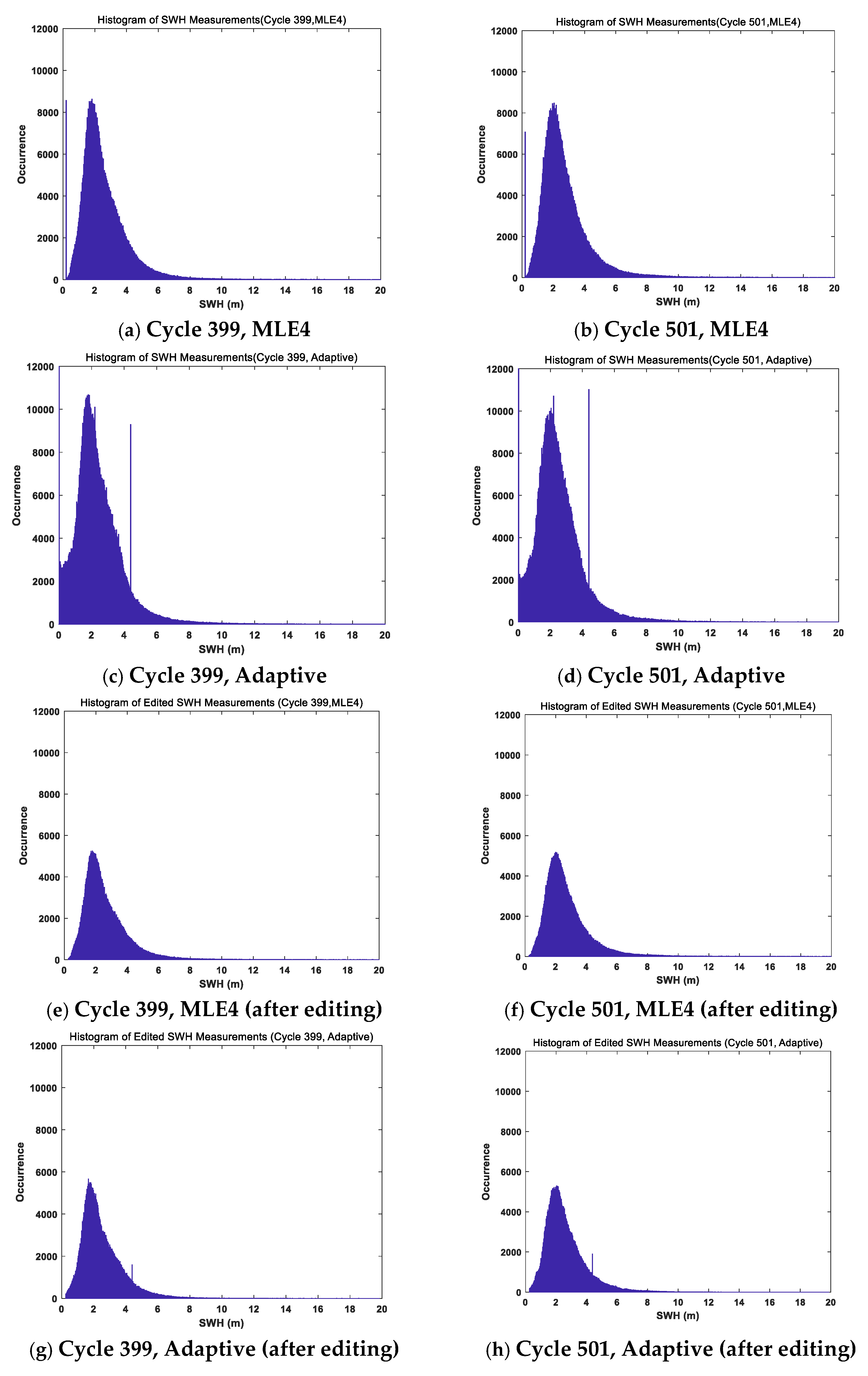
Figure 2.
Histograms of WS measurements.
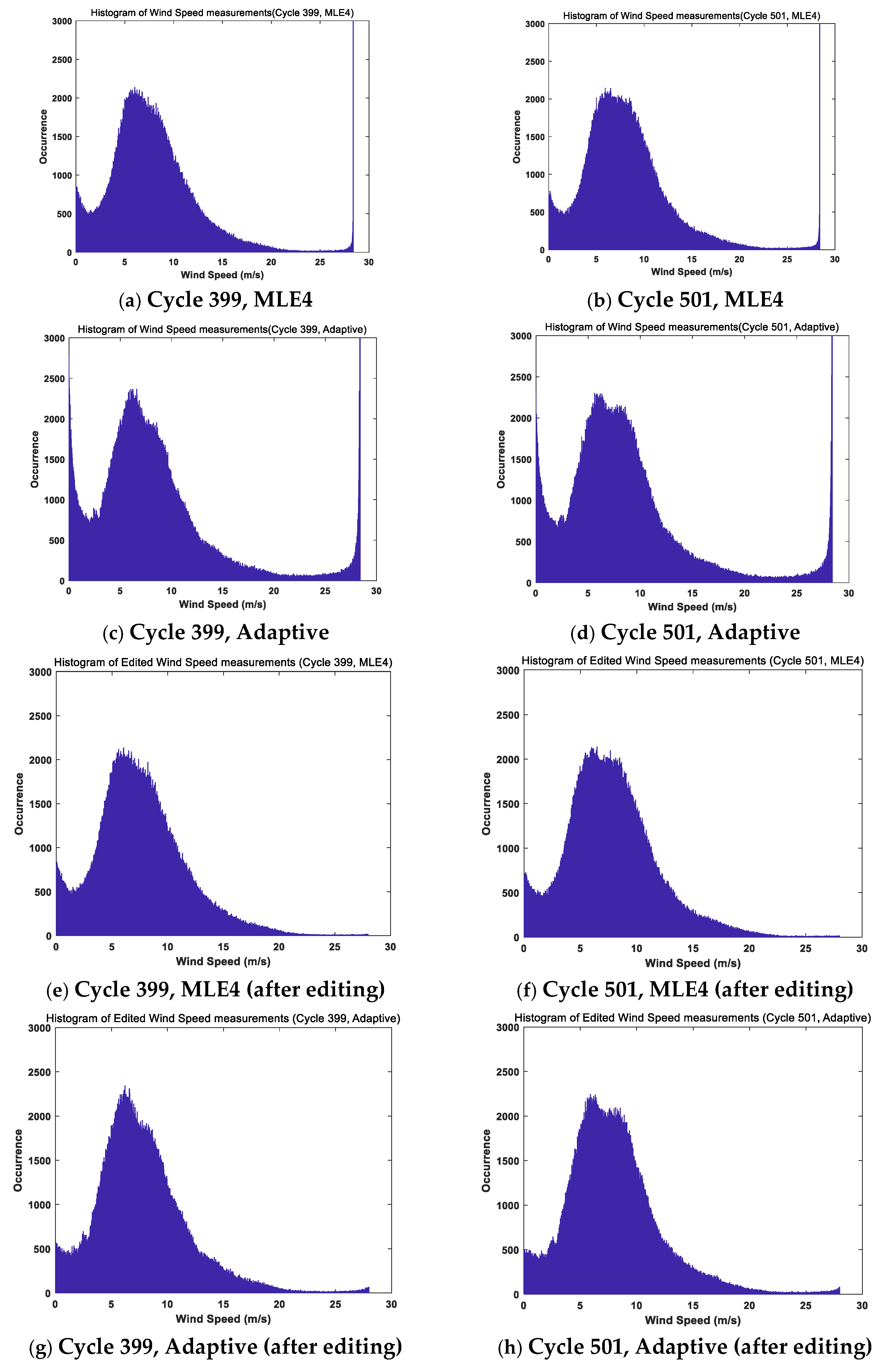

Table 1.
Evolution of the Models from Jason-3 GDR-F to Jason-3 GDR-G.
| Model | GDR-F | GDR-G |
| Orbit model | MOE/POE-F | MOE/POE-G |
| FES Ocean and load tide model | FES2014B | FES2022B |
| MSS models1 | CNES_CLS-2015 + DTU18 | Hybrid 2023 + DTU21 |
| MDT model1 | CNES_CLS_MDT-2022 | CNES_CLS_MDT-2022 |
1 GDR-G also provide accuracy parameters of the MSS and MDT models.
Table 2.
Evolution of the Models from Jason-3 GDR-F to Jason-3 GDR-G.
| Correction item | Baseline solution | Secondary solution |
| Wet tropospheric delay | Microwave radiometer | ECMWF model |
| Ionospheric delay | Dual-frequency altimetry | GIM model |
| Sea state bias | 2D model | 3D model |
| Ocean tide1 | FES model | GOT model |
| MSS | CNES_CLS (F) / Hybrid (G) | DTU model |
1 Historically, the ocean tide parameter based on the FES model has a suffix of “sol2”, but it is the data source of “ssha” computation in the data product.
Table 3.
SSHA mean values and relative biases to the baseline product under the eight strategies (Unit: centimeters; GDR-F SSHAs were averaging from cycles #394-399, and GDR-G SSHAs were averaging from cycles #501-506).
Table 3.
SSHA mean values and relative biases to the baseline product under the eight strategies (Unit: centimeters; GDR-F SSHAs were averaging from cycles #394-399, and GDR-G SSHAs were averaging from cycles #501-506).
| Strategy | GDR-F SSHA Average | ΔSSHA | GDR-G SSHA Average | ΔSSHA |
| Baseline (MLE4) | 5.40 | 0 | 5.03 | 0 |
| 3D SSB (MLE4) | 7.05 | 1.65 | 6.60 | 1.57 |
| Model wet path (MLE4) | 5.64 | 0.24 | 5.15 | 0.12 |
| GIM ionospheric (MLE4) | 6.89 | 1.48 | 6.65 | 1.62 |
| GOT tide (MLE4) | 5.43 | 0.03 | 5.06 | 0.03 |
| DTU MSS (MLE4) | 5.98 | 0.58 | 5.12 | 0.08 |
| Baseline (Adaptive) | 2.94 | -2.46 | 2.56 | -2.48 |
| 3D SSB (Adaptive) | 4.46 | -0.94 | 4.02 | -1.01 |
Table 4.
SSHA standard deviations under different strategy (Unit: centimeters, GDR-F, cycle 394-399).
Table 4.
SSHA standard deviations under different strategy (Unit: centimeters, GDR-F, cycle 394-399).
| Strategy | Cycle #394 | Cycle #395 | Cycle #396 | Cycle #397 | Cycle #398 | Cycle #399 | Average |
| Baseline (MLE4) | 5.18 | 5.17 | 5.05 | 5.05 | 5.00 | 4.94 | 5.07 |
| 3D SSB (MLE4) | 5.04 | 5.04 | 4.91 | 4.90 | 4.85 | 4.85 | 4.93 |
| Model wet tropospheric (MLE4) | 5.21 | 5.20 | 5.07 | 5.08 | 5.03 | 4.97 | 5.09 |
| GIM ionospheric (MLE4) | 5.18 | 5.18 | 5.05 | 5.05 | 5.00 | 4.95 | 5.07 |
| GOT tide (MLE4) | 5.21 | 5.21 | 5.08 | 5.09 | 5.03 | 4.98 | 5.10 |
| DTU MSS (MLE4) | 5.24 | 5.25 | 5.12 | 5.08 | 5.04 | 4.98 | 5.12 |
| Baseline (Adaptive) | 4.91 | 5.02 | 4.77 | 4.82 | 4.80 | 4.78 | 4.85 |
| 3D SSB (Adaptive) | 4.80 | 4.93 | 4.67 | 4.69 | 4.68 | 4.67 | 4.74 |
Table 5.
SSHA standard deviations under different strategy (Unit: centimeters, GDR-G, cycle 501-506).
Table 5.
SSHA standard deviations under different strategy (Unit: centimeters, GDR-G, cycle 501-506).
| Strategy | Cycle #501 | Cycle #502 | Cycle #503 | Cycle #504 | Cycle #505 | Cycle #506 | Average |
| Baseline (MLE4) | 4.92 | 5.01 | 4.99 | 5.05 | 5.00 | 4.94 | 4.99 |
| 3D SSB (MLE4) | 4.80 | 4.89 | 4.86 | 4.90 | 4.85 | 4.85 | 4.86 |
| Model wet path (MLE4) | 4.94 | 5.04 | 5.01 | 5.08 | 5.03 | 4.97 | 5.01 |
| GIM ionospheric (MLE4) | 4.93 | 5.01 | 4.99 | 5.05 | 5.00 | 4.95 | 4.99 |
| GOT tide (MLE4) | 4.96 | 5.05 | 5.03 | 5.09 | 5.03 | 4.98 | 5.02 |
| DTU MSS (MLE4) | 4.94 | 5.05 | 5.01 | 5.08 | 5.04 | 4.98 | 5.02 |
| Baseline (Adaptive) | 4.74 | 4.85 | 4.78 | 4.82 | 4.80 | 4.78 | 4.80 |
| 3D SSB (Adaptive) | 4.63 | 4.73 | 4.67 | 4.69 | 4.68 | 4.67 | 4.68 |
Table 6.
SSHA improvement or deterioration over the MEL4 baseline SSHA (Unit: centimeters, Detrend method, cycle 501-503).
Table 6.
SSHA improvement or deterioration over the MEL4 baseline SSHA (Unit: centimeters, Detrend method, cycle 501-503).
| Strategy | GDR-F | GDR-G | Improvement of GDR-G over GDR-F | ||
| Mean Detrend SSHA noise level | Improvement or deterioration over Baseline (MLE4)1 | Mean Detrend SSHA noise level | Improvement or deterioration over Baseline (MLE4)1 | ||
| Baseline (MLE4) | 5.07 | 0 | 4.99 | 0 | 0.90 |
| 3D SSB (MLE4) | 4.93 | + 1.11 | 4.86 | + 1.15 | 0.85 |
| Model wet path (MLE4) | 5.09 | - 0.52 | 5.01 | - 0.54 | 0.91 |
| GIM ionospheric (MLE4) | 5.07 | - 0.18 | 4.99 | - 0.18 | 0.90 |
| GOT tide (MLE4) | 5.10 | - 0.62 | 5.02 | - 0.60 | 0.88 |
| DTU MSS (MLE4) | 5.12 | - 0.71 | 5.02 | - 0.74 | 1.02 |
| Baseline (Adaptive) | 4.85 | + 1.36 | 4.80 | + 1.46 | 0.73 |
| 3D SSB (Adaptive) | 4.74 | + 1.72 | 4.68 | + 1.79 | 0.76 |
1 “+” in this column denotes improvement or, “-“ denotes deterioration.
Table 7.
Comparison of MLE4 SWH and Adaptive SWH.
| Cycle No. | Percentage of extremely low SWH (MLE4) | Percentage of extremely low SWH (Adaptive) | Average SWH after editing (MLE4) | Average SWH after editing (Adaptive) | SWH Difference between Adaptive and MLE4 |
| 394 | 1.17% | 9.84% | 2.76m | 2.60m | -0.16m |
| 395 | 1.02% | 9.66% | 2.78m | 2.53m | -0.25m |
| 396 | 1.03% | 8.59% | 2.74m | 2.57m | -0.17m |
| 397 | 0.95% | 7.69% | 2.75m | 2.58m | -0.17m |
| 398 | 0.90% | 6.91% | 2.87m | 2.70m | -0.17m |
| 399 | 1.03% | 6.71% | 2.69m | 2.51m | -0.18m |
| 501 | 0.84% | 5.21% | 2.81m | 2.62m | -0.19m |
| 502 | 0.91% | 5.08% | 3.03m | 2.83m | -0.20m |
| 503 | 0.96% | 5.31% | 2.81m | 2.61m | -0.20m |
| 504 | 1.07% | 5.59% | 2.90m | 2.70m | -0.20m |
| 505 | 0.89% | 5.63% | 3.02m | 2.82m | -0.20m |
| 506 | 0.99% | 6.13% | 2.84m | 2.65m | -0.19m |
Table 8.
Comparison of MLE4 Sigma-0 and Adaptive Sigma-0.
| Cycle No. | Average Sigma-0 after editing (MLE4) | Average Sigma-0 after editing (Adaptive) | Sigma-0 Difference between Adaptive and MLE4 |
| 394 | 13.90 dB | 13.71 dB | -0.19 dB |
| 395 | 13.83 dB | 13.82 dB | -0.01 dB |
| 396 | 13.86 dB | 13.66 dB | -0.20 dB |
| 397 | 13.82 dB | 13.63 dB | -0.19 dB |
| 398 | 13.75 dB | 13.56 dB | -0.19 dB |
| 399 | 13.98 dB | 13.79 dB | -0.19 dB |
| 501 | 13.79 dB | 13.59 dB | -0.20 dB |
| 502 | 13.72 dB | 13.53 dB | -0.19 dB |
| 503 | 13.85 dB | 13.64 dB | -0.21 dB |
| 504 | 13.79 dB | 13.59 dB | -0.20 dB |
| 505 | 13.72 dB | 13.53 dB | -0.19 dB |
| 506 | 13.79 dB | 13.61 dB | -0.18 dB |
Table 9.
Comparison of MLE4 WS and Adaptive WS.
| Cycle No. | Percentage of extremely high WS (MLE4) | Percentage of extremely high WS (Adaptive) | Average WS after editing (MLE4) | Average WS after editing (Adaptive) | WS Difference between Adaptive and MLE4 |
| 394 | 0.58% | 8.35% | 8.06 m/s | 8.12 m/s | + 0.06 m/s |
| 395 | 0.57% | 8.70% | 8.15 m/s | 7.86 m/s | -0.29 m/s |
| 396 | 0.57% | 8.45% | 7.99 m/s | 8.08 m/s | + 0.09 m/s |
| 397 | 0.60% | 8.71% | 8.08 m/s | 8.15 m/s | + 0.07 m/s |
| 398 | 0.62% | 8.83% | 8.22 m/s | 8.29 m/s | + 0.07 m/s |
| 399 | 0.58% | 8.74% | 7.71 m/s | 7.78 m/s | + 0.07 m/s |
| 501 | 0.69% | 9.42% | 7.88 m/s | 7.98 m/s | + 0.10 m/s |
| 502 | 0.68% | 9.44% | 8.10 m/s | 8.18 m/s | + 0.08 m/s |
| 503 | 0.69% | 9.52% | 7.79 m/s | 7.88 m/s | + 0.09 m/s |
| 504 | 0.68% | 9.48% | 8.00 m/s | 8.09 m/s | + 0.09 m/s |
| 505 | 0.65% | 9.30% | 8.06 m/s | 8.16 m/s | + 0.10 m/s |
| 506 | 0.64% | 9.36% | 7.95 m/s | 8.03 m/s | + 0.08 m/s |
Disclaimer/Publisher’s Note: The statements, opinions and data contained in all publications are solely those of the individual author(s) and contributor(s) and not of MDPI and/or the editor(s). MDPI and/or the editor(s) disclaim responsibility for any injury to people or property resulting from any ideas, methods, instructions or products referred to in the content. |
© 2025 by the authors. Licensee MDPI, Basel, Switzerland. This article is an open access article distributed under the terms and conditions of the Creative Commons Attribution (CC BY) license (http://creativecommons.org/licenses/by/4.0/).
Copyright: This open access article is published under a Creative Commons CC BY 4.0 license, which permit the free download, distribution, and reuse, provided that the author and preprint are cited in any reuse.


