
Submitted:
25 April 2025
Posted:
25 April 2025
You are already at the latest version
Abstract
Sea level rise constitutes a globally pervasive phenomenon, regional manifestations often exhibit substantial heterogeneity due to local environmental and climatic factors. In semi-enclosed basins like the Black Sea, sea level changes are marked by distinctive spatial and temporal patterns. Understanding the spatiotemporal evolution of sea level in such regions is essential for elucidating localized responses to broader climatic drivers. This study utilizes sea surface height (SSH) data derived from satellite altimetry (SA) to investigate sea level variability in the Black Sea over eight distinct time periods: 1993–2000, 1993–2003, 1993–2005, 1993–2008, 1993–2011, 1993–2013, 1993–2017, and 1993–2021 corresponding to time series durations of 7, 10, 12, 15, 18, 20, 24, and 28 years. Four noise models were applied to estimate sea level trends, uncertainties, and annual amplitudes, the optimal model was identified to characterize sea level change, revealing long-term trend, spatial variation, and seasonal variability across the basin. The results indicate that: (1) Sea level change in the Black Sea is not linear over time and exhibits spatial heterogeneity. The estimated sea level trends over eight distinct periods are 21.68 ± 4.05 mm/a, 10.61 ± 1.61 mm/a, 8.84 ± 1.62 mm/a, 3.68 ± 0.89 mm/a, 6.74 ± 0.83 mm/a, 4.14 ± 0.69 mm/a, 3.07 ± 0.61 mm/a, and 2.34 ± 0.59 mm/a, respectively; (2) These results demonstrate that sea level trends estimates are strongly dependent on the length of the observational record. Shorter time series are associated with greater variability and higher uncertainty in trend estimates, whereas longer records provide more stable and statistically robust results. Accordingly, a minimum observation period of 24 years is recommended to ensure reliable and accurate estimation of sea level trend in the region. (3) An analysis of the SSH and phase over the period 1993–2021 at virtual altimetry stations reveals that the Black Sea experiences peak annual amplitudes during the winter and early spring months, particularly in November, December, January, and February. In contrast, an examination of data from six selected tide gauge (TG) stations indicates that the maximum annual amplitude generally occurs in April-June (June, May, June, May, April, May). The discrepancy in seasonal peak timing between SA and TG derived estimates can be attributed to differences in the spatial and temporal characteristics of sea level signals. Tide gauges, situated along coastlines, are more influenced by local factors such as tidal patterns and vertical land motion, whereas satellite altimetry primarily captures basin-wide sea level variability. (4) To mitigate the uncertainty in sea level estimates induced by noise in the SSH time series, principal component analysis (PCA) was applied to denoise the SSH records for the period 1993–2021. The resulting mean sea level trend was estimated at 1.76 ± 0.56 mm/a, which is in agreement with the Copernicus Marine Service estimate of 1.4 ± 0.83 mm/a for the period 1993–2022. After PCA-based noise reduction, 96.8% of the altimetry stations exhibited a reduction in trend uncertainty, with an average decrease of 1.92 mm/a, the root means square error of SSH time series decreased by 5.06 mm, and the annual amplitude diminished by 23.35%. These results demonstrate the efficacy of PCA in suppressing noise while retaining the long-term trend and spatial characteristics of sea level change.
Keywords:
Black Sea
; sea level trend
; sea level uncertainty
; satellite altimetry
; tide gauges
1. Introduction
Sea level exhibits temporal variability attributable to both natural and anthropo-genic influences. The predominant drivers of contemporary sea-level change comprise glacier mass, tectonic activity, geoid deformation, and greenhouse gas emissions [1,2,3,4]. Against the backdrop of ongoing global warming, sea level rise has emerged as an increasingly critical global issue [5,6,7]. Since the 1990 s, the global mean sea level has been rising at an average rate of approximately 3.1 mm/a [8,9,10]. The rise in sea levels has submerged low-lying coastal zones, amplified storm surge intensity, accelerated coastal erosion and flood frequency, and imposed constraints on the socioeconomic development of littoral regions, critically jeopardizing the long-term sustainability of coastal nations and communities [11,12].
The Black Sea (Figure 1), located in the southwestern sector of Eurasia, represents the world's largest inland marine basin by surface area. This semi-enclosed sea is bounded by six littoral states—Bulgaria, Romania, Ukraine, Russia, Georgia, and Turkey—functioning as a strategic maritime nexus [13]. The Black Sea receives inflow from several major fluvial systems in Eastern Europe, the Danube, Dnieper, and Dniester rivers. Unlike open ocean basins, it is hydrologically connected to the Sea of Azov via the Kerch Strait to the north and exchanges water with the global ocean through the narrow Turkish Straits in the southwest [14,15]. The total coastline of the Black Sea measures approximately 4,090 km in length. Coastal erosion and saltwater intrusion constitute significant environmental threats to adjacent regions. Long-term sea level changes in the Black Sea have resulted in pronounced coastal transgression and regression. As marine forces increasingly impact low-lying coastal zones, the progressing erosional processes lead to the loss of beach areas, a landward displacement of the coastline, and the degradation of coastal ecosystems [16,17].
As the deepest enclosed inland sea in the world, the Black Sea has garnered considerable scientific interest due to its distinctive geographical characteristics. Investigating sea level variability in this region is crucial for comprehending its response to climate change. Early investigations employing climate models elucidated the seasonal evolution of circulation patterns and mesoscale eddies in the Black Sea [18]. The subsequent integration of multi-source observational techniques substantially enhanced measurement precision: Synergistic analyses of SA and TG records provided baseline estimates of sea level trend [19,20,21,22]. Numerous studies have further examined the physical mechanisms underlying sea level variability, including the combined influence of river discharge and atmospheric forcing [23], non-seasonal mass redistribution processes [24], the role of basin-scale dynamics in shaping spatial heterogeneity [25], and the spatiotemporal variability of wave climate [26]. Collectively, these studies offer critical theoretical and observational foundations for advancing the understanding of the driving mechanisms behind sea level change in the Black Sea. Nevertheless, further investigations are required to more effectively capture variability across multiple temporal scales and to elucidate spatial heterogeneity.
This study utilizes satellite altimetry-derived SSH data in conjunction with four distinct noise models to characterize sea level variability in the Black Sea across multiple temporal scales. The optimal noise model was selected to estimate the sea level trend, its associated uncertainty, and the annual amplitude. Furthermore, the analysis encompasses assessments of long-term trend, spatiotemporal dynamics, and seasonal variations in sea level. To reduce the impact of noise inherent in the SSH time series, PCA was employed to reduce noise and enhance the accuracy of sea level change estimation.
2. Materials and Methods
2.1. Satellite Altimetry Products
The Copernicus Marine Environment Monitoring Service (CMEMS) provides high-precision, multi-satellite merged altimetry products that encompass both global and regional oceanic domains [27,28]. These datasets have been extensively utilized in scientific research and operational ocean forecasting. By integrating observations from multiple satellite missions and implementing rigorous quality control and data assimilation procedures, CMEMS altimetry products ensure both temporal consistency and spatial reliability. In this study, we employed the GLOB-AL_MULTIYEAR_PHY_001_030 product (https://doi.org/10.48670/moi-00021),which span the period from January 1993 to December 2020. This dataset offers a daily temporal resolution and a horizontal spatial resolution of 0.083° × 0.083°. Its high spatiotemporal fidelity renders it particularly suitable for studies of ocean circulation, assessments of climate variability, and analyses of long-term sea level trend. The dataset provides a reliable foundation for investigating a range of physical oceanographic processes.
2.2. Noise Model Theory
SA time series are characterized by the presence of long-term trend, seasonal components, and stochastic variability. Precise identification of the underlying noise structure is essential for producing robust trend estimates and for quantifying parameter uncertainties with statistical confidence. To enhance the accuracy of trend estimation, we introduce appropriate noise models. In this study, four distinct noise models are evaluated, and data modeled under the optimal noise structure are employed for subsequent analyses.
2.2.1. AutoRegressive Fractionally Integrated Moving Average
ARFIMA noise model, an extension of the classical ARIMA framework. The key feature of ARFIMA lies in its generalization of the differencing order to non-integer values, enabling a more accurate representation of long-range dependence in time series data [29,30]. The definition of the ARFIMA noise model is [31]:
is the backshift operator (), is the residual at time (observation minus modelled signal) and is a white noise signal.
2.2.2. AutoRegressive Moving Average
ARMA noise model is widely used for modeling stationary time series, incorporating both autoregressive and moving average components. By combining the autoregressive (AR) and moving average (MA) processes, the ARMA model effectively captures the autocorrelation structure inherent in time series data [32].
where and are model order parameters, are auto-regressive parameters, are moving average parameters, and satisfies the white noise assumption.
2.2.3. Generalized Gauss Markov
Sea level time series errors often exhibit temporal correlation [33,34]. The GGM framework accommodates temporal correlations by permitting the error terms to exhibit a structured, typically non-diagonal, covariance matrix. Within this context, the generalized least squares method can be employed to derive statistically efficient and unbiased parameter estimates [35]. The analytical expression for the autocovariance vector (with = 1) for this noise model is [36]:
is the fractional differencing order, represents the autoregressive coefficient, is the Gauss hypergeometric function.
2.2.4. White Noise
WN is a sequence of uncorrelated and identically distributed random variables, used to represent random perturbations with zero mean, constant variance, and no correlation across time. It can be expressed as , where is the noise at time . In the case of white noise with unit variance ( = 1), the covariance matrix reduces to the identity matrix [37].
2.3. Principal Component Analysis Denoising Method
PCA is a linear transformation-based technique widely used for data dimensionality reduction and noise mitigation [38]. Its core principle involves projecting high-dimensional data onto a new orthogonal coordinate system via eigen decomposition, such that the variance along each principal component is maximized [39]. In ocean remote sensing applications, this characteristic is particularly effective for noise suppression: principal components associated with larger eigenvalues typically capture large-scale signal variations, whereas those corresponding to smaller eigenvalues predominantly contain noise-related features [40,41]. The mathematical implementation involves three key steps:
- The raw SSH data are subjected to standard preprocessing, including mean centering and variance normalization.is the original sequence matrix, is the average sea level at each time point.
- constructing the covariance matrix and performing eigenvalue de-composition.
- Eigenvalue decomposition is performed to decompose the covariance matrix of the standardized SSH data into its eigenvalues and corresponding eigenvectors [42,43].The eigenvalue represents the contribution of the corresponding principal component, while the eigenvector defines its orientation in the original variable space.
- The standardized data are projected onto the principal component space by multiplying the original anomaly matrix with a subset of leading eigenvectors [44]. This step retains only the principal components associated with the largest eigenvalues, which capture the dominant modes of variability, while effectively filtering out high-frequency noise and less significant variations.
- Reconstruct the data by selecting the principal components corresponding to the first largest eigenvalues.containing the directions of the first principal components, is the SSH time series matrix reconstructed after retaining the principal components.
PCA can effectively project the SSH time series into a low-dimensional signal subspace, thereby filtering out small-scale noise components and significantly improving the signal-to-noise ratio of the observed data.
3. Results
3.1. Impact of Time Series Length on Balck Sea Level Change Estimation
Since 1993, SA has been extensively utilized for monitoring global sea level changes [45,46,47]. To investigate the effects of coastal proximity and spatial heterogeneity on regional sea level estimation, this study employs a virtual altimetry station methodology [48]; a ring of stations positioned along the outer margin of the Black Sea coastline, then incrementally extended inward toward the basin's interior until the entire sea area was adequately covered. Ultimately, a total of 406 virtual altimetry stations were identified for analysis (Figure 2).
Previous studies have demonstrated that SA observations are affected by various types of noise, which can degrade the precision of sea level trend estimations and increase the uncertainty in estimates of sea level change [49,50]. To mitigate the impact of such noise and more accurately extract long-term trend, this study employed four noise models—ARFIMA(1, d, 1), ARMA(1,1), GGM, and WN. The optimal model for each time interval was identified using the BIC_tp [51]. Previous studies have also demonstrated that the duration of the observational time series exerts a substantial influence on the accuracy of sea level trend estimations [52]. To investigate the temporal evolution of sea level in the Black Sea and evaluate the effect of time period on trend estimation, sea level change and their associated uncertainties were estimated for eight different time periods. To assess the robustness of the results, the derived sea level trends were compared with those reported in previous literature over comparable periods, and both consistencies and discrepancies were examined (Table 1).
The results of this study indicate that the Black Sea experienced a significant upward trend in sea level during 1993-2000, with an estimated trend of 21.68 ± 4.05 mm/a.This result is in good agreement with the conclusion of a study based on the Centre National d’Etudes Spatiales /AVISO satellite altimetry data (27.30 ± 2.50 mm/a during 1993–1998) [53]. Cazenave et al. [53] pointed out that the abnormal sea level rise during this period may be driven by multiple factors, including the expansion of the surface water body due to heating and the reduction of the runoff of major rivers into the sea, which led to a positive water balance and weakened the seasonal sea level fluctuations.
This study determined that the sea level trend in the Black Sea during 1993–2005 was 8.84 ± 1.62 mm/a, which falls within the uncertainty range of the estimate reported by a previous study (7.60 ± 0.30 mm/a) [20], based on TG records and SA data provided by the Division for Space Oceanography of Collecte Localisation Satellites. Kubryakov and Stanichnyi [20] attributed this relatively elevated trend to decadal-scale sea level variability and highlighted the pronounced spatial heterogeneity of sea level change across the Black Sea basin.
During the period 1993–2013, the sea level trend in the Black Sea was estimated in this study to be 4.14 ± 0.69 mm/a. This estimate is in reasonable agreement with the result reported by a previous study [25], who derived a rate of 3.15 ± 0.13 mm/a for the period 1993–2014 using daily sea level anomaly data from AVISO altimetry. Kubryakov et al. [25] indicated that variations in the mean sea level of the Black Sea are primarily governed by its water balance. Moreover, the observed spatial heterogeneity in sea level is closely linked to the basin’s internal dynamical processes.
This study estimated a sea level rise rate of 3.07 ± 0.61 mm/a in the Black Sea during the period 1993–2017. Avsar and Kutoğlu [54] based on daily SSH data provided by CMEMS, estimated the mean sea level rise in the Black Sea to be 2.50 ± 0.50 mm/a after removing seasonal cycles from the SSH time series. The study also highlighted the significant interannual variability in the non-seasonal sea level changes in the Black Sea.
The estimated sea level trend in this study is 2.34±0.59 mm/a for 1993-2021, and the CMEMS estimated the Black Sea sea level trend to be 1.40±0.83 mm/a for 1993-2022 based on the OMI_CLIMATE_SL_BLKSEA_area_averaged_anomalies product (https://doi.org/10.48670/moi-00215). The CMEMS estimate was corrected for TOPEX-A instrumental drift and basin-averaged glacial isostatic adjustment (GIA), and further processed by removing seasonal, annual, and semi-annual signals, followed by low-pass filtering to isolate long-term trend.
A comparative analysis reveals that the characteristics of sea level change exhibit temporal variability across different periods. Within the same time period, our estimates generally align with those reported in existing studies, although some discrepancies are evident. These differences may be attributed to variations in the SA data products and the methods used for station selection. For instance, Kubryakov and Stanichnyi [20] utilized a dataset specifically tailored for the Black Sea, characterized by a temporal resolution of 10 days and a spatial resolution of 7 km, to estimate sea level trend over 1993-2005, based on station data located along satellite altimetry tracks. Kubryakov et al. [25] used regional grid data of sea level anomalies to estimate sea level change over the period 1993–2014. The sea level trend data for the Black Sea provided by CMEMS during 1993–2022 are based on a dedicated satellite altimetry dataset for the Black Sea and account for the effects of GIA. In general, sea level change in the Black Sea do not follow a strictly linear pattern. While the long-term trend indicates an upward trajectory, the rate of change exhibits variability across different time periods. During the period 1993–2000, the sea level trend was as high as 21.68 mm/a, but this trend slowed afterward, with the rate of change fluctuating between 2 and 8 mm/a after 2005.
3.2. Analysis of Sea Level Trend Uncertainty in the Black Sea
To evaluate the impact of time series length on the accuracy of sea level trend estimation, this study investigates the uncertainties in sea level trend across eight distinct time periods (Table 2).
The uncertainty of the trend is influenced by both the duration of the observational time series and the presence of noise, with its magnitude serving as an indicator of the stability and reliability of the estimated trend. Figure 3 shows the spatial variability in trend of uncertainty over different periods.
The uncertainty of sea level trend estimation decreases progressively with the extension of the time span, leading to more accurate and stable estimates (Figure 4). In contrast, short-term time series exhibit greater variability in trend estimation. This is primarily because sea level trends are sensitive to interannual and decadal variability, making it difficult for short records to distinguish long-term signals from short-term fluctuations, thereby increasing the uncertainty of trend estimates [49]. In the semi-enclosed Black Sea, sea level variability is also influenced by regional climate conditions and oceanic circulation. Short observational time series may fail to capture the full extent of these changes, and relying on a limited number of SA observations can result in substantial uncertainties in trend estimation [20]. In contrast, long-term time series effectively suppress the influence of interannual and decadal variations, resulting in more reliable trend estimates [56]. In light of our findings, we recommend utilizing time series exceeding 24 years in length to enhance the robustness and accuracy of sea level trend estimations.
3.3. Spatial Variation of Sea Level Trend in the Black Sea
To further investigate the spatial distribution characteristics of sea level change in the Black Sea, this study utilizes SA data spanning the period 1993–2021, using sea level trends estimated from 406 virtual satellite stations under their respective optimal noise models, a spatial distribution map of sea level trend in the Black Sea region was generated through geospatial interpolation techniques (Figure 5).
Figure 5 illustrates spatial variability in sea level trend across the Black Sea, with trend ranging from 0.41 mm/a to 4.22 mm/a throughout the basin. Long-term change in the Black Sea’s dynamic regime influence the spatial distribution of sea level trend within the region [25].Previous studies have identified water balance as the dominant driver of long-term sea level change in the Black Sea [57]. Along the western coast, inflows from major rivers such as the Danube and Dnieper affect local sea levels, primarily through variations in river discharge. The maximum sea level trend 4.22 mm/a is observed in the southwestern sector of the basin, adjacent to the Turkish Straits. This region is subject to dynamic influences from water exchange through the straits and is modulated by the topographic constraints of the continental shelf; strong wind events can alter the net flow through the straits, subsequently impacting sea level [58]. Furthermore, studies have shown that the highest average significant wave heights also occur in this southwestern zone near the Turkish coast [59], indicating that the sea level change in this area are more significant due to the influence of dynamic factors. In contrast, the southeastern Black Sea displays lower sea level trend compared to other regions, which may be associated with the presence of anticyclonic gyres. Cyclonic and anticyclonic gyres can induce regional water accumulation or depletion, thereby modulating sea level variability in the area [60].
3.4. Seasonal Change in the Black Sea
Due to localized oceanographic processes, sea level changes across different regions of the Black Sea basin exhibit marked spatial heterogeneity. In semi-enclosed basins such as the Black Sea, sea level variability is neither temporally linear nor spatially uniform [61]. Sea level changes are influenced not only by long-term trend but also by short-term variability, including seasonal climatic fluctuations, ocean circulation patterns, wind stress, and thermohaline structure [62]. This study investigates the characteristics of seasonal variability in the Black Sea by analyzing annual amplitude across eight different time periods. According to the statistical results (Table 3), the annual amplitudes remain relatively stable over time, with only minor fluctuations between intervals. A slight decreasing trend in amplitude is observed with increasing temporal coverage, which may be associated with evolving climate patterns, adjustments in ocean circulation, or interannual variability.
To further explore the spatial characteristics of seasonal oscillations, a spatial distribution map of annual amplitudes for the period 1993–2021 was generated (Figure 6), highlighting regional disparities in seasonal sea level variability across the basin.
The annual amplitude of sea level variation of the Black Sea is not uniformly distributed. Higher amplitudes are observed along the northeastern and southern coasts compared to the central basin. This spatial pattern may be attributed to the cyclonic boundary currents and basin-scale dynamics, which tend to elevate coastal sea levels [63,64]. Seasonal amplitude is further enhanced by local storm surges and Ekman transport, both of which are influenced by prevailing wind patterns [25]. In contrast, the interior basin, constrained by the semi-enclosed nature of the Black Sea, exhibits relatively lower amplitudes. Seasonal sea level variations are modulated by multiple factors, including atmospheric pressure fluctuations, wind stress, river discharge, water balance, and oceanic dynamics. To further investigate the characteristics of seasonal variability and the timing of sea level maxima, this study analyzed SA-derived SSH time series at 406 virtual altimetry stations over the 28-year period from 1993 to 2021, identifying the months in which peak sea levels occur (Table 4).
Statistical analysis reveals that peak sea levels at most stations occur predominantly in December and January, comprising 27.63% and 28.06% of occurrences, respectively (Figure 7). This seasonal pattern aligns with the dynamics of freshwater inflow, as the Black Sea basin typically experiences the highest precipitation during the winter months, coupled with peak river discharge in the spring. The combined effects of increased winter precipitation and intensified river inflow during spring likely contribute to elevated sea levels observed in December and January. Aydın and Beşiktepe [65] reported that the highest sea levels generally occur between spring and summer, while the lowest levels are observed during autumn when river discharge is minimal. Sea level variability in the Black Sea has also been shown to be influenced by the North Atlantic Oscillation (NAO), which regulates terrestrial water storage and indirectly contributes to sea level fluctuations [23,66]. Sea level fluctuations in the Black Sea exhibit a negative correlation with the NAO index, with elevated sea levels typically occurring during negative NAO phases [67], during this phases, increased precipitation and river runoff enhance freshwater input into the basin, while intensified wind forcing can reduce outflow through the Bosphorus Strait, further amplifying sea level rise.
To investigate the spatiotemporal characteristics, dynamic evolution, and seasonal patterns of the annual amplitude of sea level variability in the Black Sea, this study analyzes the phase values derived from 406 virtual altimetry stations for the period 1993–2021. Statistical analysis identifies the calendar month corresponding to the maximum annual amplitude at each station (Table 5), revealing the temporal distribution pattern of peak annual sea level variability across the Black Sea.
The results (Figure 8) indicate that the maximum annual amplitude at the majority of virtual altimetry stations occurs in January, February, November, and December, collectively accounting for 77.59% of all stations. This pattern aligns with the months during which peak sea levels are observed. In addition, six TG stations were selected from the Permanent Service for Mean Sea Level (PSMSL) to analyze their phase values. The study period is consistent with that reported in the literature [54], and the geographical location of TG is shown in the Figure 9.
According to the results (Table 6), the months of maximum annual amplitude at the six TG stations are June, May, June, May, April, and May, respectively, which are consistent with the findings [68]. In contrast, most altimetry stations exhibit their peak annual amplitudes in January, February, November, and December. Discrepancies between virtual altimetry and TG station observations are likely driven by interannual and short-term variability in coastal sea levels. Differences in spatial and temporal sampling between TG and SA observations can introduce inconsistencies in the derived sea level time series [69]. Additionally, TG stations are located along the coastline and are influenced by local tidal regimes and vertical land motion [22], while SA data represent broader, basin-wide sea level variability.
4. Discussion
SA provides a reliable means to detect sea level change since 1993. However, short observational records are insufficient to capture interannual and decadal variability, which limits the accuracy of long-term sea level trend estimations. To assess the influence of time series length on sea level change, we analyzed the spatial characteristics of sea level trend in the Black Sea over eight different periods. The results reveal notable differences in the trend patterns across these periods, underscoring the non-stationary and regionally heterogeneous nature of sea level change within the basin (Figure 10).
During the period 1993–2000, the Black Sea exhibited relatively large fluctuations in sea level trend. After 2005, the sea level trend exhibited a decline. Previous studies have indicated that sea level variations in this region are closely linked to the discharge of the Danube River during the same period [15]. In contrast, the trend observed over the longer intervals of 1993–2013, 1993–2017, and 1993–2021 display a more stable pattern, further reinforcing the conclusion that longer time series provide more reliable and consistent estimates of sea level trend. Since sea level estimation is often influenced by noise interference, regional variability, and measurement uncertainties, the SSH time series derived from SA data typically contain colored noise, which compromises the accuracy of the estimates [70]. Seasonal changes in sea level will also affect the accurate estimation of sea level trend, especially short time series estimation is more affected. To improve the accuracy of sea level change estimation in the Black Sea, this study applies PCA to denoise the SSH time series over the period 1993–2021. PCA can extract and remove the main seasonal patterns to reduce the interference of seasonal changes on sea level estimation. Figure 11 illustrates a comparison of the SSH time series at SA Station 1 before and after the denoising process.
As illustrated in the time series plots, the SSH data subjected to PCA-based denoising exhibit a smoother temporal evolution with diminished short-term variability, thereby facilitating a more robust identification of long-term sea level trend. The denoised time series were subsequently utilized to estimate sea level trend over the Black Sea. To evaluate the impact of PCA-based denoising on trend estimation, we constructed spatial distribution maps of sea level trend for the period 1993–2021 (Figure 12), along with a station comparison of trend estimates before and after denoising (Figure 13).
Accurate estimation of sea level trends depends critically on the stability of long-term signals. To further assess the effectiveness of PCA-based denoising, we investigated its influence on the uncertainty associated with sea level trend estimates(Figure 14).
PCA was applied to denoise the SSH time series at 406 virtual altimetry stations across the Black Sea for the period 1993–2021. The resulting mean sea level trend after PCA processing was 1.76 ± 0.56 mm/a, which is consistent with the CMEMS’s estimate of 1.40 ± 0.83 mm/a for the period 1993–2022. On average, trend changed by 0.57 mm/a following denoising, while the original spatial and temporal characteristics of the trend were effectively preserved. Notably, 96.8% of the altimetry stations exhibited a reduction in trend uncertainty, with an average decrease of 1.92 mm/a (Figure 15). Furthermore, the root mean square error of SSH, decreased by an average of 5.06 mm after PCA denoising. Additionally, the mean annual amplitude was reduced from 19.23 ± 5.99 mm to 14.74 ± 6.97 mm, reflecting a 23.35% reduction. These confirm that PCA effectively mitigates noise while preserving the underlying trend, thus enhancing the reliability of sea level estimates in the Black Sea.
5. Conclusions
This study investigates the temporal and spatial variability of sea level change in the Black Sea based on SA data. By analyzing sea level trend, trend of uncertainty, and annual amplitude under an optimized noise model across multiple time periods, the research highlights both the spatial heterogeneity and seasonal patterns of sea level variability. To address the challenge of high uncertainty in sea level trend estimates, PCA was applied to denoise the SSH time series. This approach enabled a more accurate and robust estimation of long-term sea level trend in the Black Sea.
(1) The study quantified sea level trend in the Black Sea over eight progressively longer time periods under an optimal noise model: 1993–2000, 1993–2003, 1993–2005, 1993–2008, 1993–2011, 1993–2013, 1993–2017, and 1993–2021, with corresponding rates of 21.68 ± 4.05 mm/a, 10.61 ± 1.61 mm/a, 8.84 ± 1.62 mm/a, 3.68 ± 0.89 mm/a, 6.74 ± 0.83 mm/a, 4.14 ± 0.69 mm/a, 3.07 ± 0.61 mm/a, and 2.34 ± 0.59 mm/a, respectively. The results indicate a consistent decrease in trend uncertainty as the time series length increases. In contrast, shorter time series are more vulnerable to interannual and decadal oceanic variability, which can introduce significant biases into trend estimation. Consequently, it is recommended that time series of at least 24 years be utilized for sea level trend estimation in the Black Sea to improve the accuracy and reliability of the results. Shorter time series are more susceptible to interannual and decadal variability, which can bias trend assessments. Spatial analyses further reveal a heterogeneous sea level response across the basin, likely influenced by the Black Sea’s semi-enclosed nature, the presence of cyclonic boundary currents, and regional climate forcing such as the NAO, which collectively affect the basin’s water balance and drive spatially variable sea level changes.
(2) An analysis of the phase values from 406 virtual altimetry stations over the period 1993–2021 revealed that the months of peak annual amplitude predominantly occur in winter and early spring (November, December, January, and February). This is consistent with the finding that the maximum sea level at the SA stations predominantly occurs in December and January. In contrast, the peak phases derived from six TG stations obtained from the PSMSL were found to occurs in April-June (June, May, June, May, April, May). The discrepancy between SA and TG observations is likely attributable to differences in observational methodologies and the influence of interannual variability inherent to the Black Sea system. Notably, TG stations are located along the coast and are subject to localized influences, including tidal patterns and land motion, whereas SA measurements reflect broader, basin-wide sea level dynamics.
(3) To accurately estimate sea level change in the Black Sea, PCA was applied to the 1993–2021 SSH time series from 406 virtual altimetry stations for noise reduction. This approach successfully preserved the original sea level trend and spatial distribution characteristics. After noise reduction, the sea level trend in the Black Sea for the period 1993–2021 was estimated at 1.76 ± 0.56 mm/a, consistent with the results reported by the CMEMS. The application of PCA reduced the trend uncertainty by an average of 1.92 mm/a, while the root means square error decreased by an average of 5.06 mm. Additionally, the annual amplitude decreased by 23.35%.
Author Contributions
Original draft and data processing, Y.F. and X.S.; methodology, X.H.; reviewed the manuscript, S.H.; created some plots, J.Z., J.W. and Y.L. All authors have read and agreed to the published version of the manuscript.
Funding
This work is funding by 2024 National College Students' Innovation and Entrepreneurship Training Program Project (202410407026), National Natural Science Foundation China (42364002), Major Discipline Academic and Technical Leaders Training Program of Jiangxi Province (20225BCJ23014), Key Research and Development Program Project of Jiangxi Province (20243BBI91033), Post-doctoral Later-stage Foundation Project of Shenzhen Polytechnic University (P-20211230–00004) and Shenzhen Polytechnic Research Fund (6023310006K).
Data Availability Statement
The ocean reanalysis data used in this study are available from the Copernicus Marine Service. Specifically, the Global Ocean Physics Reanalysis product (product ID:GLOBAL_MULTIYEAR_PHY_001_030) provides global temperature, salinity, sea surface heigh, and covers the time period from January 1993 to December 2020. The data can be accessed freely via the Copernicus Marine Environment Monitoring Ser-vice(https://data.marine.copernicus.eu/product/GLOBAL_MULTIYEAR_PHY_001_030/description). The tide gauge data used in this study are available from the Permanent Service for Mean Sea Level (https://www.psmsl.org/data/).
Conflicts of Interest
The authors declare no conflicts of interest.
Abbreviations
| SA | Satellite altimetry |
| TG | Tide gauge |
| SSH | Sea surface heigh |
| PCA | Principal component analysis |
| CMEMS | Copernicus Marine Service |
| ARFIMA | AutoRegressive Fractionally Integrated Moving Average |
| ARMA | AutoRegressive Moving Average |
| GGM | Generalized Gauss Markov |
| WN | White Noise |
| NAO | North Atlantic Oscillation |
| PSMSL | Permanent Service for Mean Sea Level |
| GIA | Glacial isostatic adjustment |
References
- Church, J.A., Gregory, J.M., Huybrechts, P., Kuhn, M., Lambeck, K., Nhuan, M.T., Qin, D. and Woodworth, P.L., 2001. Changes in sea level. In , in: JT Houghton, Y. Ding, DJ Griggs, M. Noguer, PJ Van der Linden, X. Dai, K. Maskell, and CA Johnson (eds.): Climate Change 2001: The Scientific Basis: Contribution of Working Group I to the Third Assessment Report of the Intergovernmental Panel (pp. 639-694).
- Stammer, D., Cazenave, A., Ponte, R.M. and Tamisiea, M.E., 2013. Causes for contemporary regional sea level changes. Annual review of marine science, 5(1), pp.21-46.
- Carson, M., Köhl, A., Stammer, D., A. Slangen, A.B., Katsman, C.A., W. van de Wal, R.S., Church, J. and White, N., 2016. Coastal sea level changes, observed and projected during the 20th and 21st century. Climatic Change, 134, pp.269-281.
- Huang, J., Feng, W., Yang, Y., Xiong, Y., Yang, M. and Zhong, M., 2025. Significant impact of non-tidal oceanic and atmospheric mass variations on regional ocean mass budgets: A comparative analysis across 19 representative regions. Journal of Geophysical Research: Oceans, 130(4), p.e2024JC021477.
- Dasgupta, S., Laplante, B., Meisner, C., Wheeler, D. and Yan, J., 2009. The impact of sea level rise on developing countries: a comparative analysis. Climatic change, 93(3), pp.379-388.
- Nerem, R.S., Chambers, D.P., Choe, C. and Mitchum, G.T., 2010. Estimating mean sea level change from the TOPEX and Jason altimeter missions. Marine Geodesy, 33(S1), pp.435-446.
- Roy, P., Pal, S.C., Chakrabortty, R., Chowdhuri, I., Saha, A. and Shit, M., 2023. Effects of climate change and sea-level rise on coastal habitat: Vulnerability assessment, adaptation strategies and policy recommendations. Journal of Environmental Management, 330, p.117187.
- Church, J.A. and White, N.J., 2011. Sea-level rise from the late 19th to the early 21st century. Surveys in geophysics, 32, pp.585-602.
- Ablain, M., Legeais, J.F., Prandi, P., Marcos, M., Fenoglio-Marc, L., Dieng, H.B., Benveniste, J. and Cazenave, A., 2017. Satellite altimetry-based sea level at global and regional scales. In Integrative study of the mean sea level and its components (pp. 9-33). Cham: Springer International Publishing.
- Cazenave, A. and Moreira, L., 2022. Contemporary sea-level changes from global to local scales: a review. Proceedings of the Royal Society A, 478(2261), p.20220049.
- Nicholls, R.J., Lincke, D., Hinkel, J., Brown, S., Vafeidis, A.T., Meyssignac, B., Hanson, S.E., Merkens, J.L. and Fang, J., 2021. A global analysis of subsidence, relative sea-level change and coastal flood exposure. Nature Climate Change, 11(4), pp.338-342.
- Khojasteh, D., Glamore, W., Heimhuber, V. and Felder, S., 2021. Sea level rise impacts on estuarine dynamics: A review. Science of The Total Environment, 780, p.146470.
- Poulos, S.E., 2020. The Mediterranean and Black Sea Marine System: An overview of its physico-geographic and oceanographic characteristics. Earth-Science Reviews, 200, p.103004.
- Bakan, G. and Büyükgüngör, H., 2000. The black sea. Marine pollution bulletin, 41(1-6), pp.24-43.
- Kostianoy, A.G. and Kosarev, A.N. eds., 2008. The Black Sea Environment. Springer-Verlag Berlin Heidelberg.
- Demirkesen, A.C., Evrendilek, F. and Berberoglu, S., 2008. Quantifying coastal inundation vulnerability of Turkey to sea-level rise. Environmental Monitoring and Assessment, 138, pp.101-106.
- Görmüş, T., Ayat, B., Aydoğan, B. and Tătui, F., 2021. Basin scale spatiotemporal analysis of shoreline change in the Black Sea. Estuarine, Coastal and Shelf Science, 252, p.107247.
- Stanev, E.V. and Peneva, E.L., 2001. Regional sea level response to global climatic change: Black Sea examples. Global and Planetary Change, 32(1), pp.33-47.
- Korotaev, G.K., Saenko, O.A. and Koblinsky, C.J., 2001. Satellite altimetry observations of the Black Sea level. Journal of Geophysical Research: Oceans, 106(C1), pp.917-933.
- Kubryakov, A.A. and Stanichnyi, S.V., 2013. The Black Sea level trends from tide gages and satellite altimetry. Russian Meteorology and Hydrology, 38, pp.329-333.
- Avsar, N.B., Kutoglu, S.H., Jin, S. and Erol, B., 2015. Investigaton of sea level change along the Black Sea coast from tide gauge and satellite altimetry. The International Archives of the Photogrammetry, Remote Sensing and Spatial Information Sciences, 40, pp.67-71.
- Avsar, N.B., Jin, S., Kutoglu, H. and Gurbuz, G., 2016. Sea level change along the Black Sea coast from satellite altimetry, tide gauge and GPS observations. Geodesy and Geodynamics, 7(1), pp.50-55.
- Volkov, D.L. and Landerer, F.W., 2015. Internal and external forcing of sea level variability in the Black Sea. Climate dynamics, 45, pp.2633-2646.
- Volkov, D.L., Johns, W.E. and Belonenko, T.V., 2016. Dynamic response of the Black Sea elevation to intraseasonal fluctuations of the Mediterranean sea level. Geophysical Research Letters, 43(1), pp.283-290.
- Kubryakov, A.A., Stanichny, S.V. and Volkov, D.L., 2017. Quantifying the impact of basin dynamics on the regional sea level rise in the Black Sea. Ocean Science, 13(3), pp.443-452.
- Causio, S., Federico, I., Jansen, E., Mentaschi, L., Ciliberti, S.A., Coppini, G. and Lionello, P., 2024. The Black Sea near-past wave climate and its variability: a hindcast study. Frontiers in Marine Science, 11, p.1406855.
- Law-Chune, S., Aouf, L., Dalphinet, A., Levier, B., Drillet, Y. and Drevillon, M., 2021. WAVERYS: a CMEMS global wave reanalysis during the altimetry period. Ocean Dy-namics, 71, pp.357-378.
- Sun, X., Lu, T. and Wang, Z., 2024. COMPARATIVE ANALY-SIS OF DIFFERENT DEEP LEARNING ALGORITHMS FOR THE PREDICTION OF MARINE ENVIRONMENTAL PARAMETERS BASED ON CMEMS PRODUCTS. Acta Geodynamica et Geomaterialia, 21(4), pp.343-363.
- Granger, C.W. and Joyeux, R., 1980. An introduction to long-memory time series models and fractional differencing. Journal of time series analysis, 1(1), pp.15-29.
- Beran, J., 1995. Maximum likelihood estimation of the differencing parameter for in-vertible short and long memory autoregressive integrated moving average mod-els. Journal of the Royal Statistical Society: Series B (Methodological), 57(4), pp.659-672.
- Sowell, F., 1992. Maximum likelihood estimation of stationary univariate fractionally integrated time series models. Journal of econometrics, 53(1-3), pp.165-188.
- Shumway, R.H., Stoffer, D.S. and Stoffer, D.S., 2000. Time series analysis and its applica-tions (Vol. 3, p. 4). New York: springer.
- Feng, X. and Schulteis, J., 1993, March. Iden-tification of high noise time series signals using hybrid ARMA modeling and neural network approach. In IEEE International Conference on Neural Networks (pp. 1780-1785). IEEE.
- Harville, D., 1976. Extension of the Gauss-Markov theorem to include the estimation of random effects. The Annals of Statistics, 4(2), pp.384-395.
- Williams, S.D.P., 2003. The effect of coloured noise on the uncertainties of rates estimated from geodetic time series. Journal of Geodesy, 76, pp.483-494.
- Langbein, J., 2004. Noise in two-color electronic distance meter measurements revisit-ed. Journal of Geophysical Research: Solid Earth, 109(B4).
- Moffat, I.U. and Akpan, E.A., 2019. White noise analysis: A measure of time series model adequacy. Applied Mathematics, 10(11), pp.989-1003.
- Roweis, S., 1997. EM algorithms for PCA and SPCA. Advances in neural information processing systems, 10.
- Ringnér, M., 2008. What is principal component analysis?. Nature biotechnology, 26(3), pp.303-304.
- He, X., Hua, X., Yu, K., Xuan, W., Lu, T., Zhang, W. and Chen, X., 2015. Accuracy enhancement of GPS time series using principal component analysis and block spatial filtering. Advances in Space Research, 55(5), pp.1316-1327.
- Abdi, H. and Williams, L.J., 2010. Principal component analysis. Wiley interdisciplinary reviews: computational statistics, 2(4), pp.433-459.
- Dong, D., Fang, P., Bock, Y., Webb, F., Prawirodirdjo, L., Kedar, S. and Jamason, P., 2006. Spatiotemporal filtering using principal component analysis and Karhunen-Loeve expansion approaches for regional GPS network analysis. Journal of geophysical research: solid earth, 111(B3).
- Greenacre, M., Groenen, P.J., Hastie, T., d’Enza, A.I., Markos, A. and Tuzhilina, E., 2022. Principal component analysis. Nature Reviews Methods Primers, 2(1), p.100.
- Maćkiewicz, A. and Ratajczak, W., 1993. Principal components analysis (PCA). Computers & Geosciences, 19(3), pp.303-342.
- Cazenave, A. and Moreira, L., 2022. Contemporary sea-level changes from global to local scales: A review, P. Roy. Soc. A-Math. Phy., 478, 20220049 [online.
- Guérou, A., Meyssignac, B., Prandi, P., Ablain, M., Ribes, A. and Bignalet-Cazalet, F., 2023. Current observed global mean sea level rise and acceleration estimated from satellite altimetry and the associated measurement uncertainty. Ocean Science, 19(2), pp.431-451.
- Adebisi, N., Balogun, A.L., Min, T.H. and Tella, A., 2021. Advances in estimating Sea Level Rise: A review of tide gauge, satellite altimetry and spatial data science approaches. Ocean & Coastal Management, 208, p.105632.
- Cazenave, A., Gouzenes, Y., Birol, F., Leger, F., Passaro, M., Calafat, F.M., Shaw, A., Nino, F., Legeais, J.F., Oelsmann, J. and Restano, M., 2022. Sea level along the world’s coastlines can be measured by a network of virtual altimetry stations. Communications earth & environment, 3(1), p.117.
- Bos, M.S., Williams, S.D.P., Araújo, I.B. and Bastos, L., 2014. The effect of temporal correlated noise on the sea level rate and acceleration uncertainty. Geophysical Journal International, 196(3), pp.1423-1430.
- Royston, S., Watson, C.S., Legrésy, B., King, M.A., Church, J.A. and Bos, M.S., 2018. Sea-level trend uncertainty with Pacific climatic variability and temporally-correlated noise. Journal of Geophysical Research: Oceans, 123(3), pp.1978-1993.
- He, X., Bos, M.S., Montillet, J.P. and Fernandes, R.M.S., 2019. Investigation of the noise properties at low frequencies in long GNSS time series. Journal of Geode-sy, 93(9), pp.1271-1282.
- Sun, X., Lu, T., Hu, S., Huang, J., He, X., Montillet, J.P., Ma, X. and Huang, Z., 2023. The relationship of time span and missing data on the noise model estimation of GNSS time series. Remote Sensing, 15(14), p.3572.
- Cazenave, A., Bonnefond, P., Mercier, F., Dominh, K. and Toumazou, V., 2002. Sea level variations in the Mediterranean Sea and Black Sea from satellite altimetry and tide gauges. Global and Planetary Change, 34(1-2), pp.59-86.
- Avsar, N.B. and Kutoğlu, Ş.H., 2020. Recent sea level change in the Black Sea from satellite altimetry and tide gauge observations. ISPRS International Journal of Geo-Information, 9(3), p.185.
- Feng, G., Jin, S. and Zhang, T., 2013. Coastal sea level changes in Europe from GPS, tide gauge, satellite altimetry and GRACE, 1993–2011. Advances in Space Research, 51(6), pp.1019-1028.
- Zhang, X. and Church, J.A., 2012. Sea level trends, interannual and decadal variability in the Pacific Ocean. Geophysical research letters, 39(21).
- Medvedev, I.P., 2022. Numerical Modeling of Meteorological Sea Level Oscillations in the Black Sea. Oceanology, 62(4), pp.471-481.
- Jarosz, E., Teague, W.J., Book, J.W. and Beşiktepe, Ş.T., 2012. Observations on the characteristics of the exchange flow in the Dardanelles Strait. Journal of Geophysical Research: Oceans, 117(C11).
- Rusu, L., 2019. The wave and wind power potential in the western Black Sea. Renewable energy, 139, pp.1146-1158.
- Kubryakov, A.A. and Stanichny, S.V., 2011. Mean Dynamic Topography of the Black Sea, computed from altimetry, drifter measurements and hydrology data. Ocean Science, 7(6), pp.745-753.
- Meli, M., Camargo, C.M., Olivieri, M., Slangen, A.B. and Romagnoli, C., 2023. Sea-level trend variability in the Mediterranean during the 1993–2019 period. Frontiers in Marine Science, 10, p.1150488.
- Chen, J.L., Wilson, C.R., Tapley, B.D., Famiglietti, J.S. and Rodell, M., 2005. Seasonal global mean sea level change from satellite altimeter, GRACE, and geophysical models. Journal of Geodesy, 79, pp.532-539.
- Blatov, A.S., Bulgakov, N.P., Ivanov, V.A., Kosarev, A.N. and Tujilkin, V.S., 1984. Vari-ability of hydrophysical fields in the Black Sea.
- Stanev, E.V., 1990. On the mecha-nisms of the Black Sea circulation. Earth-Science Reviews, 28(4), pp.285-319.
- Aydın, M. and Beşiktepe, Ş.T., 2022. Mechanism of generation and propagation characteristics of coastal trapped waves in the Black Sea. Ocean Science Discussions, 2022, pp.1-21.
- Wegwerth, A., Plessen, B., Kleinhanns, I.C. and Arz, H.W., 2021. Black Sea hydroclimate and coupled hydrology was strongly controlled by high-latitude glacial climate dynamics. Communications Earth & Environment, 2(1), p.63.
- Ozgenc Aksoy, A., 2017. Investigation of sea level trends and the effect of the north atlantic oscillation (NAO) on the black sea and the eastern mediterranean sea. Theoretical and Applied Climatology, 129, pp.129-137.
- Avsar, N.B., Kutoglu, S.H., Jin, S. and Erol, B., 2015. Investigaton of sea level change along the Black Sea coast from tide gauge and satellite altimetry. The International Archives of the Photogrammetry, Remote Sensing and Spatial Information Sciences, 40, pp.67-71.
- White, N.J., Church, J.A. and Gregory, J.M., 2005. Coastal and global averaged sea level rise for 1950 to 2000. Geophysical Research Letters, 32(1).
- Ablain, M., Meyssignac, B., Zawadzki, L., Jugier, R., Ribes, A., Spada, G., Benveniste, J., Cazenave, A. and Picot, N., 2019. Uncertainty in satellite estimates of global mean sea-level changes, trend and acceleration. Earth System Science Data, 11(3), pp.1189-1202.
Figure 1.
Geographical location of the Black Sea.
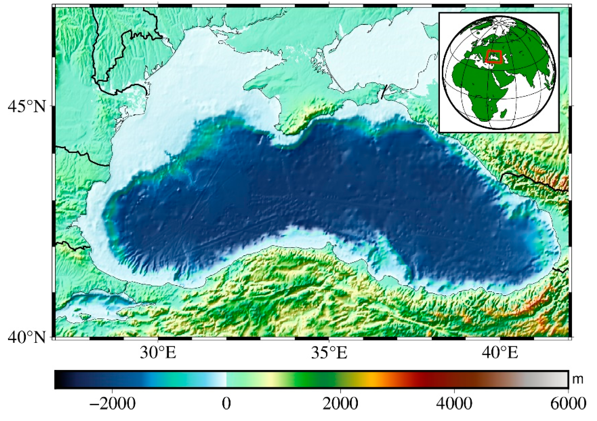
Figure 2.
Spatial distribution of virtual altimetry stations across the Black Sea. Each marker represents the geographic location of a virtual station utilized in this study for the assessment of regional sea level variability.
Figure 2.
Spatial distribution of virtual altimetry stations across the Black Sea. Each marker represents the geographic location of a virtual station utilized in this study for the assessment of regional sea level variability.
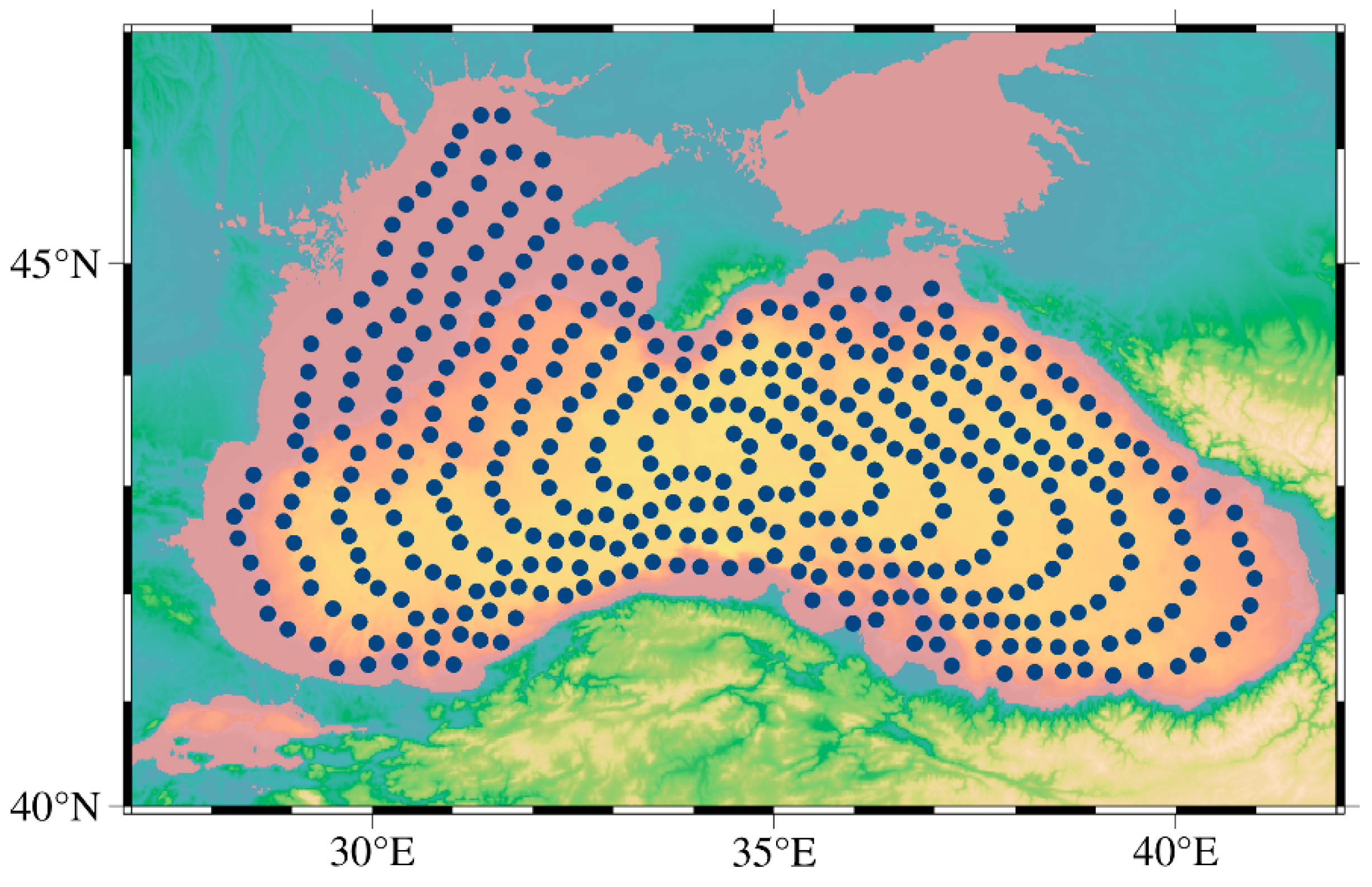
Figure 3.
Uncertainty of sea level trend (Where A, B, C, D, E, F, G and H are the uncertainties of the Black Sea level trend in 1993-2000, 1993-2003, 1993-2005, 1993-2008, 1993-2011, 1993-2013, 1993-2017, and 1993-2021).
Figure 3.
Uncertainty of sea level trend (Where A, B, C, D, E, F, G and H are the uncertainties of the Black Sea level trend in 1993-2000, 1993-2003, 1993-2005, 1993-2008, 1993-2011, 1993-2013, 1993-2017, and 1993-2021).
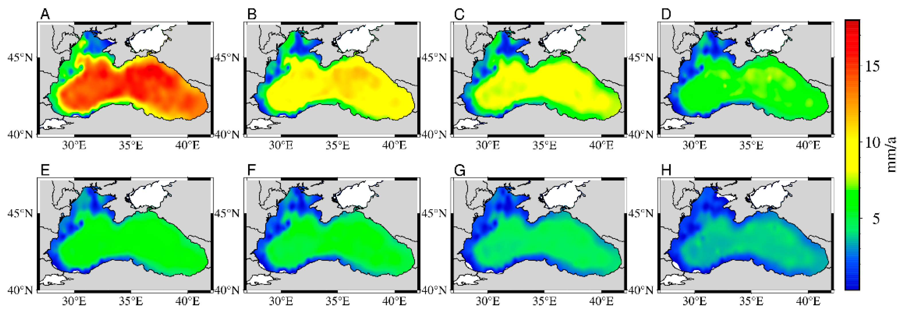
Figure 4.
Temporal evolution of sea level trend uncertainty.
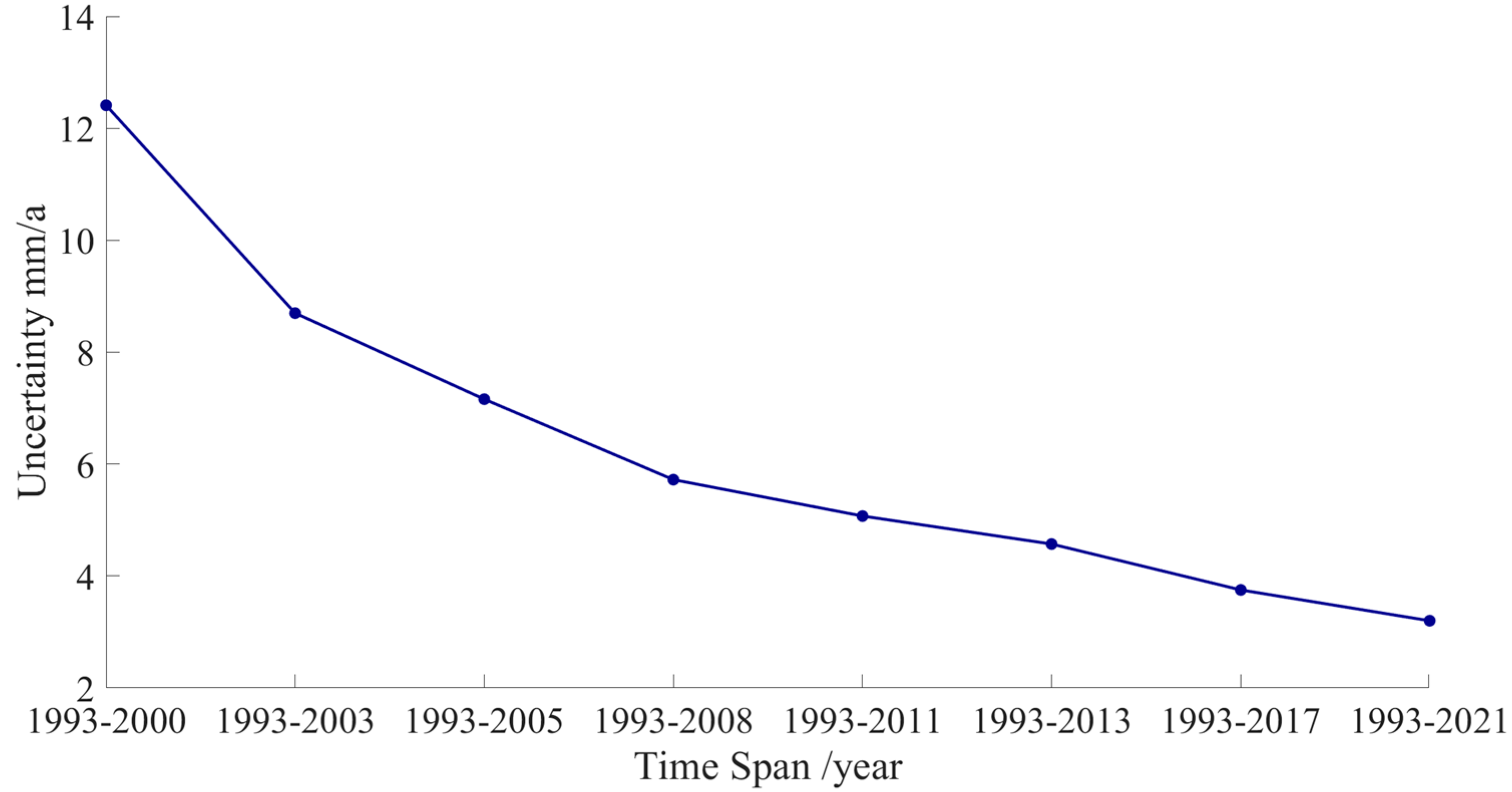
Figure 5.
Spatial variation of sea level trend in the Black Sea over the period 1993–2021.
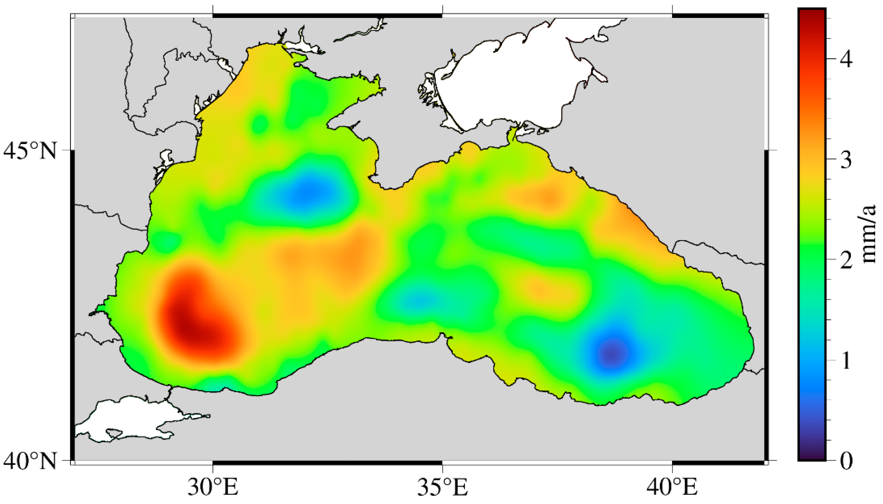
Figure 6.
Spatial distribution of annual amplitude in the Black Sea over the period 1993–2021.
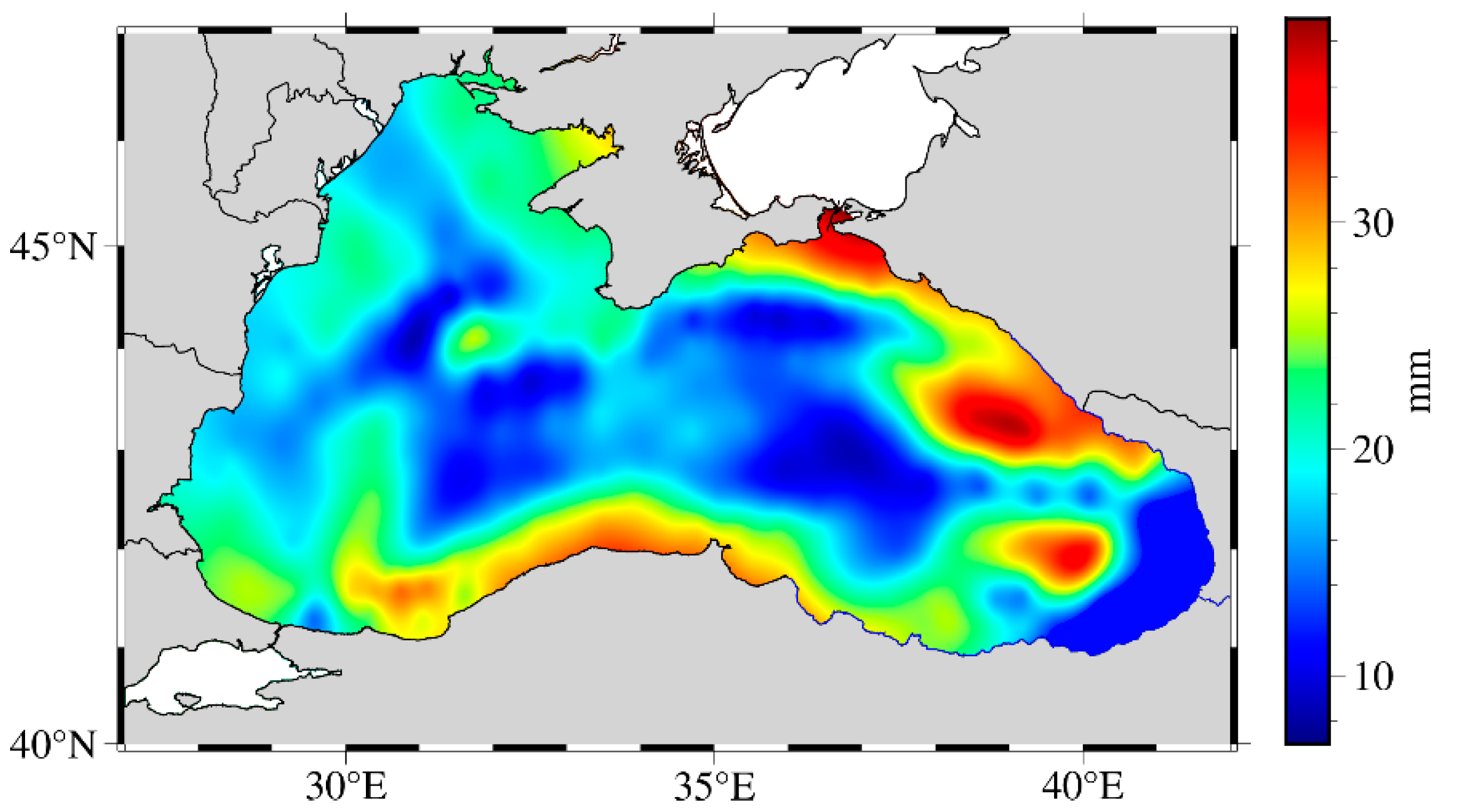
Figure 7.
Peak monthly percentages of virtual altimetry stations in the Black Sea.
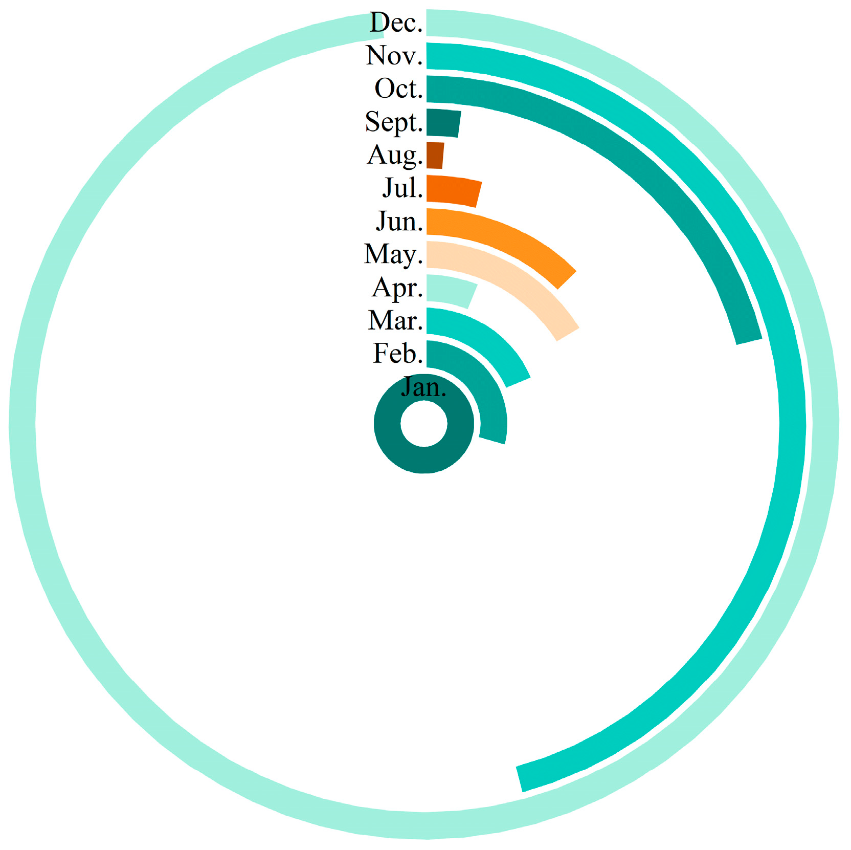
Figure 8.
Phase distribution of 406 virtual altimetry stations in the Black Sea.
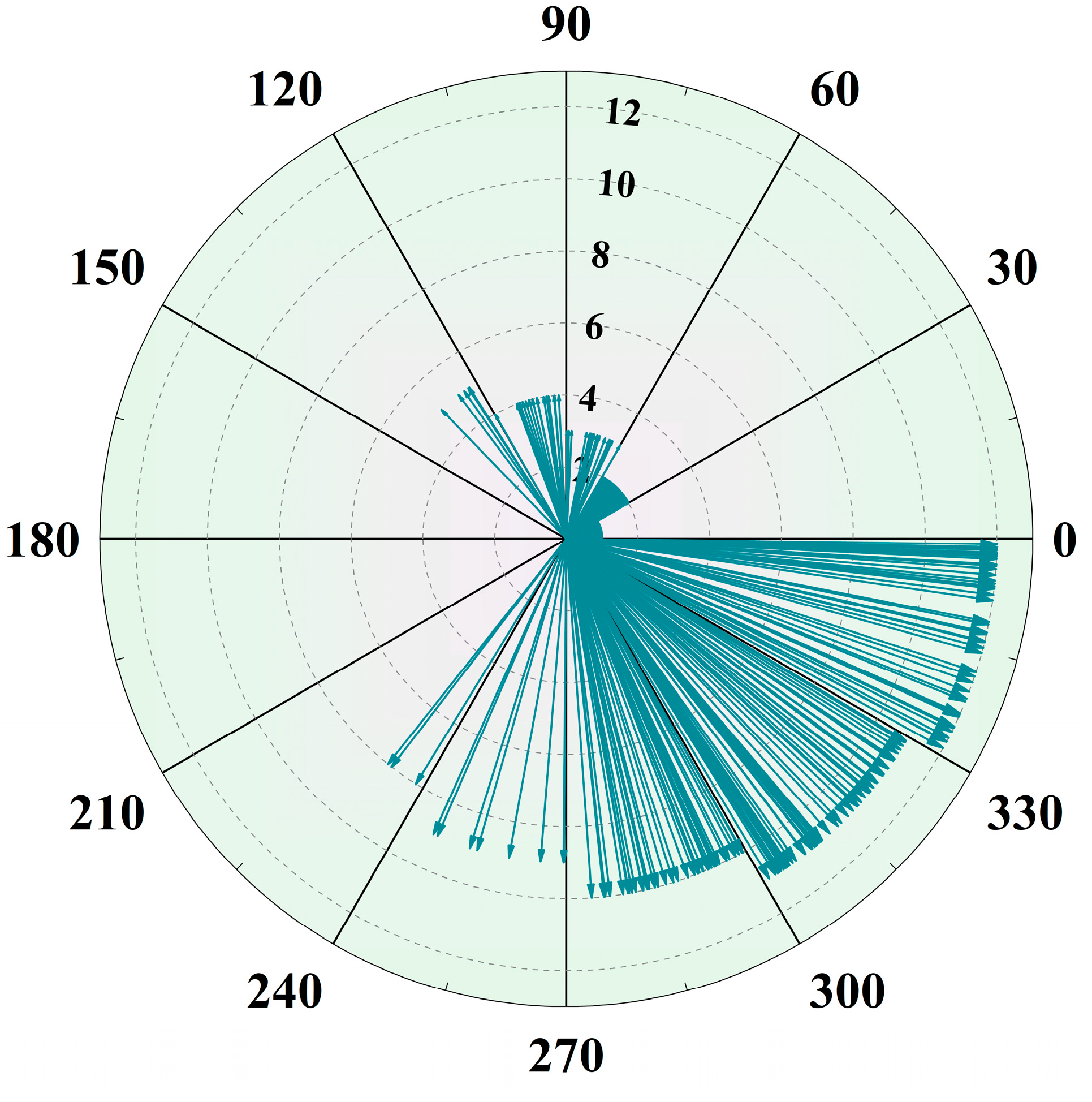
Figure 9.
The geographical location of the six TG stations selected for the study.
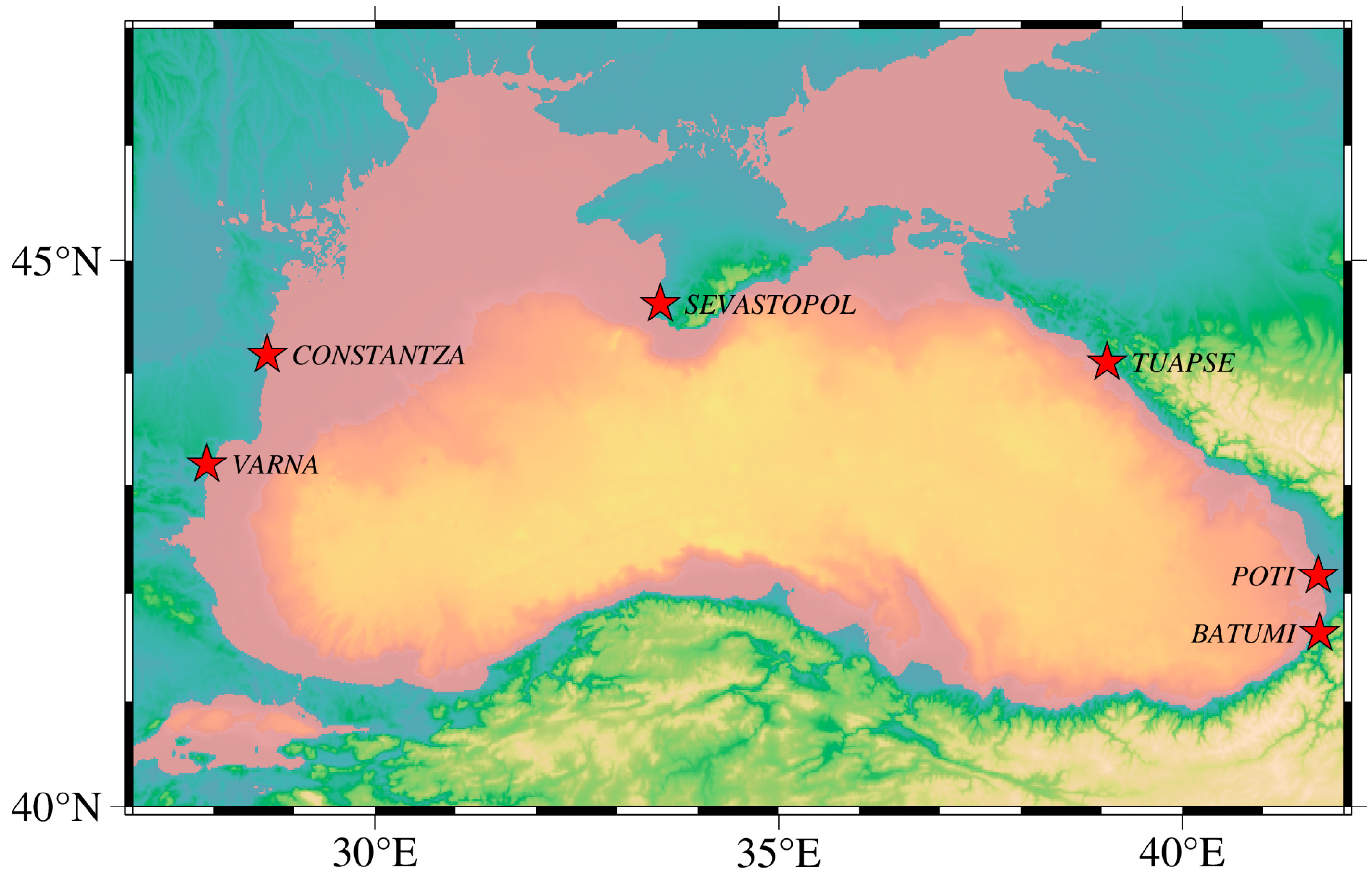
Figure 10.
Spatial distribution of sea level trend in the Black Sea over different time periods (Where A, B, C, D, E, F, G and H represent the sea level trend in 1993-2000, 1993-2003, 1993-2005, 1993-2008, 1993-2011, 1993-2013, 1993-2017, 1993-2021).
Figure 10.
Spatial distribution of sea level trend in the Black Sea over different time periods (Where A, B, C, D, E, F, G and H represent the sea level trend in 1993-2000, 1993-2003, 1993-2005, 1993-2008, 1993-2011, 1993-2013, 1993-2017, 1993-2021).
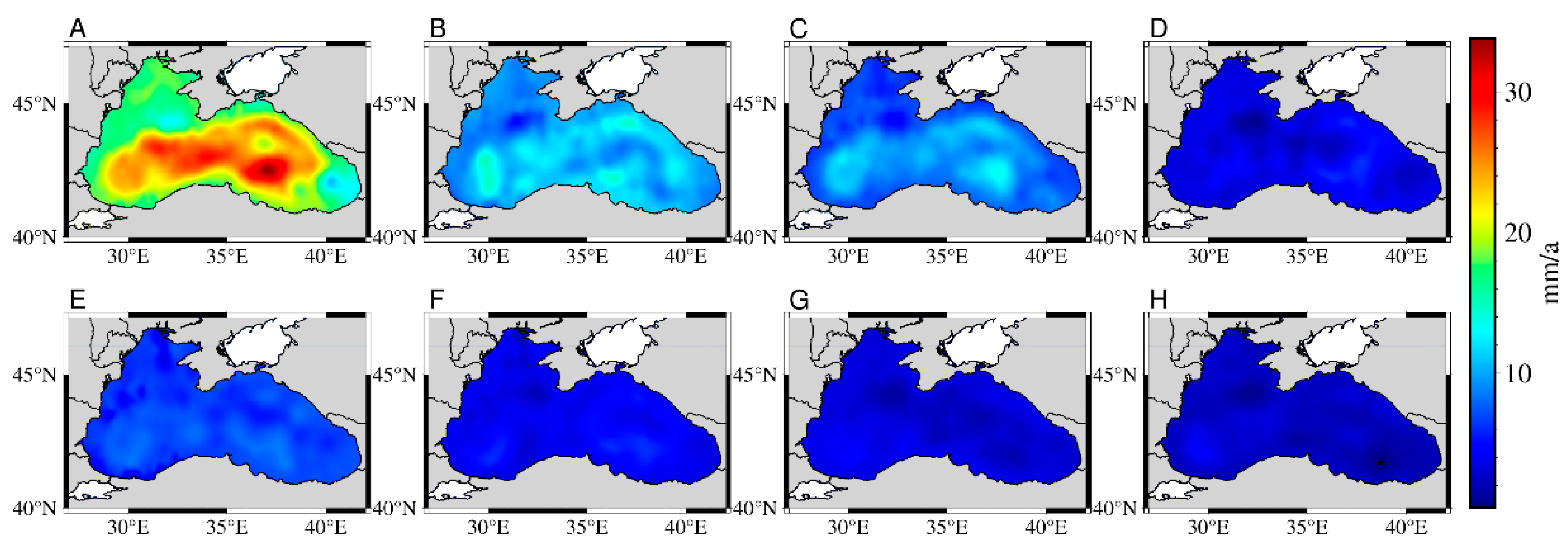
Figure 11.
Comparison of SSH time series before and after noise reduction at station 1.
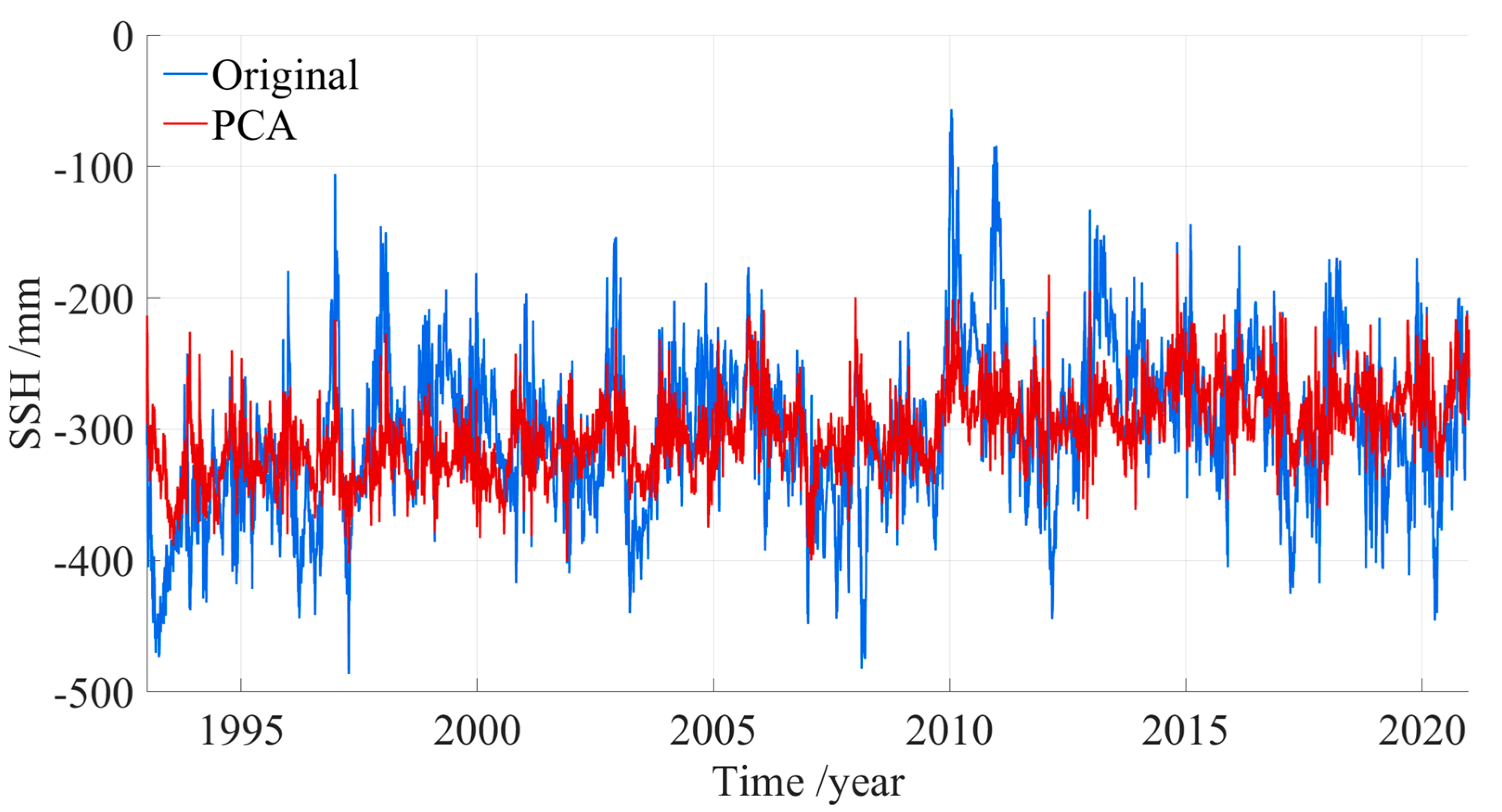
Figure 12.
Spatial distribution of sea level trend in the Black Sea over the period 1993–2021, before and after PCA processing (Where panel A is the sea level trend before PCA denoising, panel B is after PCA denoising).
Figure 12.
Spatial distribution of sea level trend in the Black Sea over the period 1993–2021, before and after PCA processing (Where panel A is the sea level trend before PCA denoising, panel B is after PCA denoising).
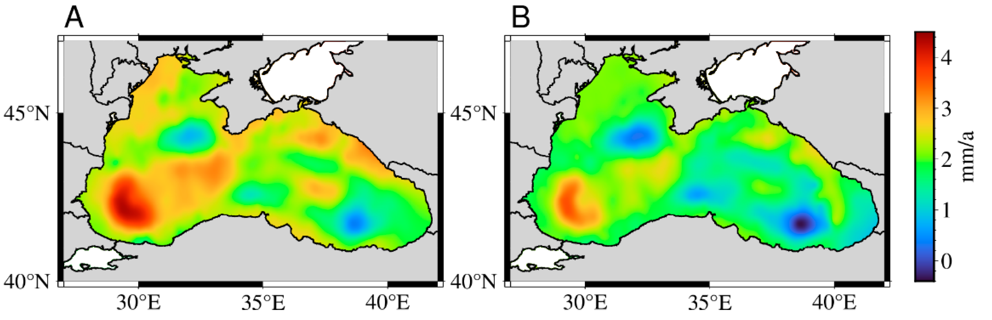
Figure 13.
Comparison of sea level trend before and after noise reduction.
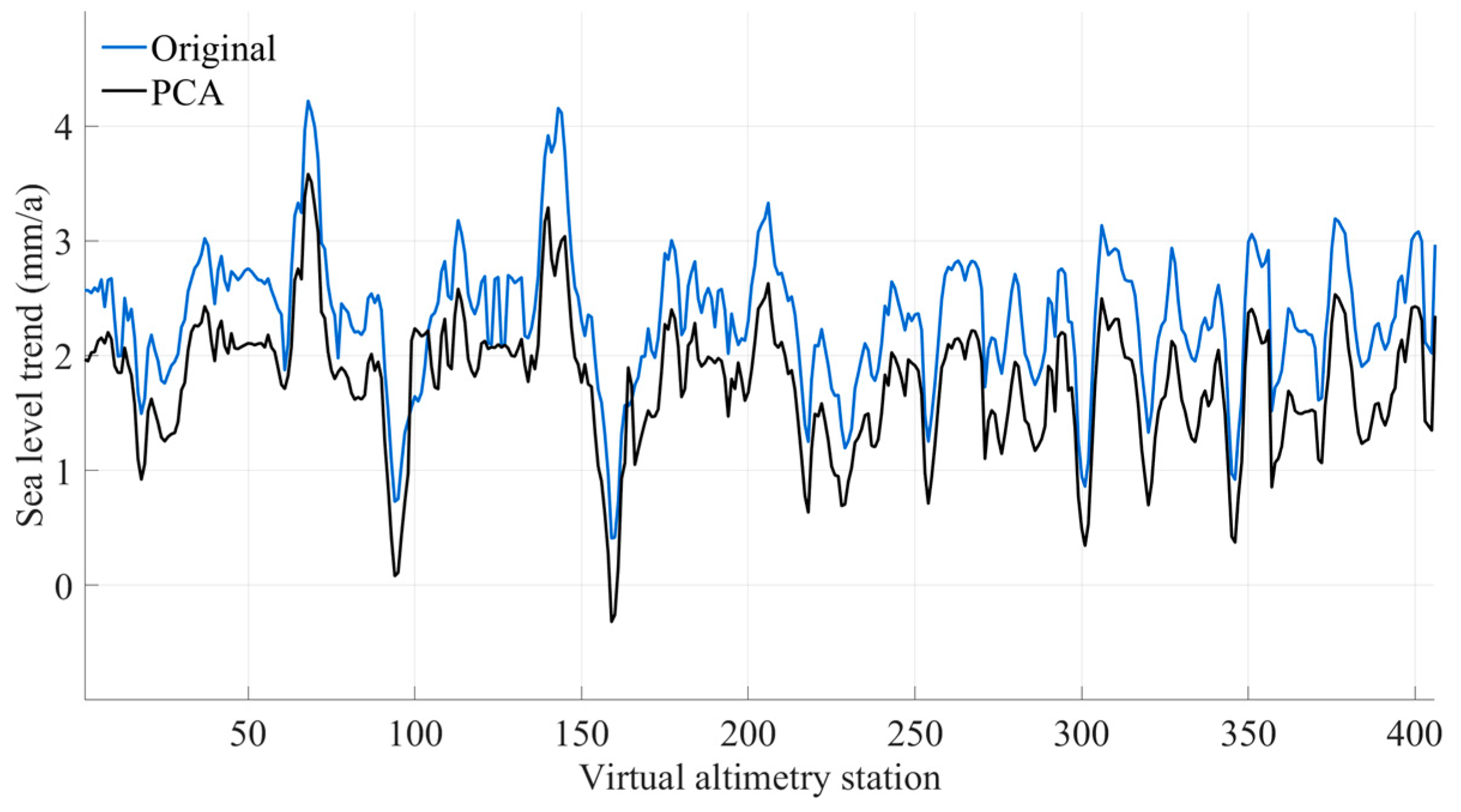
Figure 14.
Spatial distribution of sea level trend uncertainties in the Black Sea over the period 1993–2021, before and after PCA processing (Where panel A shows the uncertainties before PCA denoising, and panel B represents the uncertainties after denoising).
Figure 14.
Spatial distribution of sea level trend uncertainties in the Black Sea over the period 1993–2021, before and after PCA processing (Where panel A shows the uncertainties before PCA denoising, and panel B represents the uncertainties after denoising).
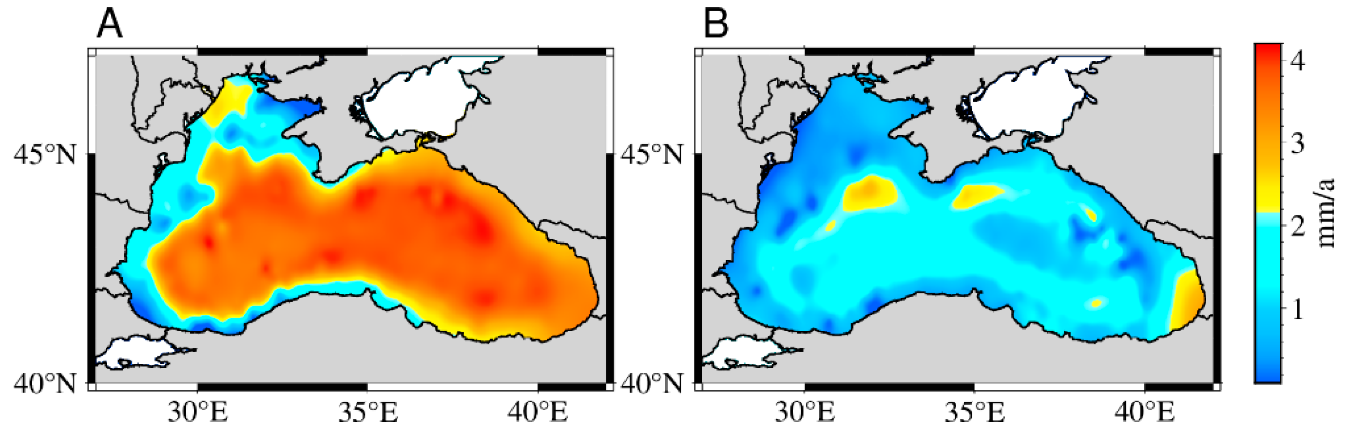
Figure 15.
Comparison of sea level trend uncertainties before and after noise reduction.
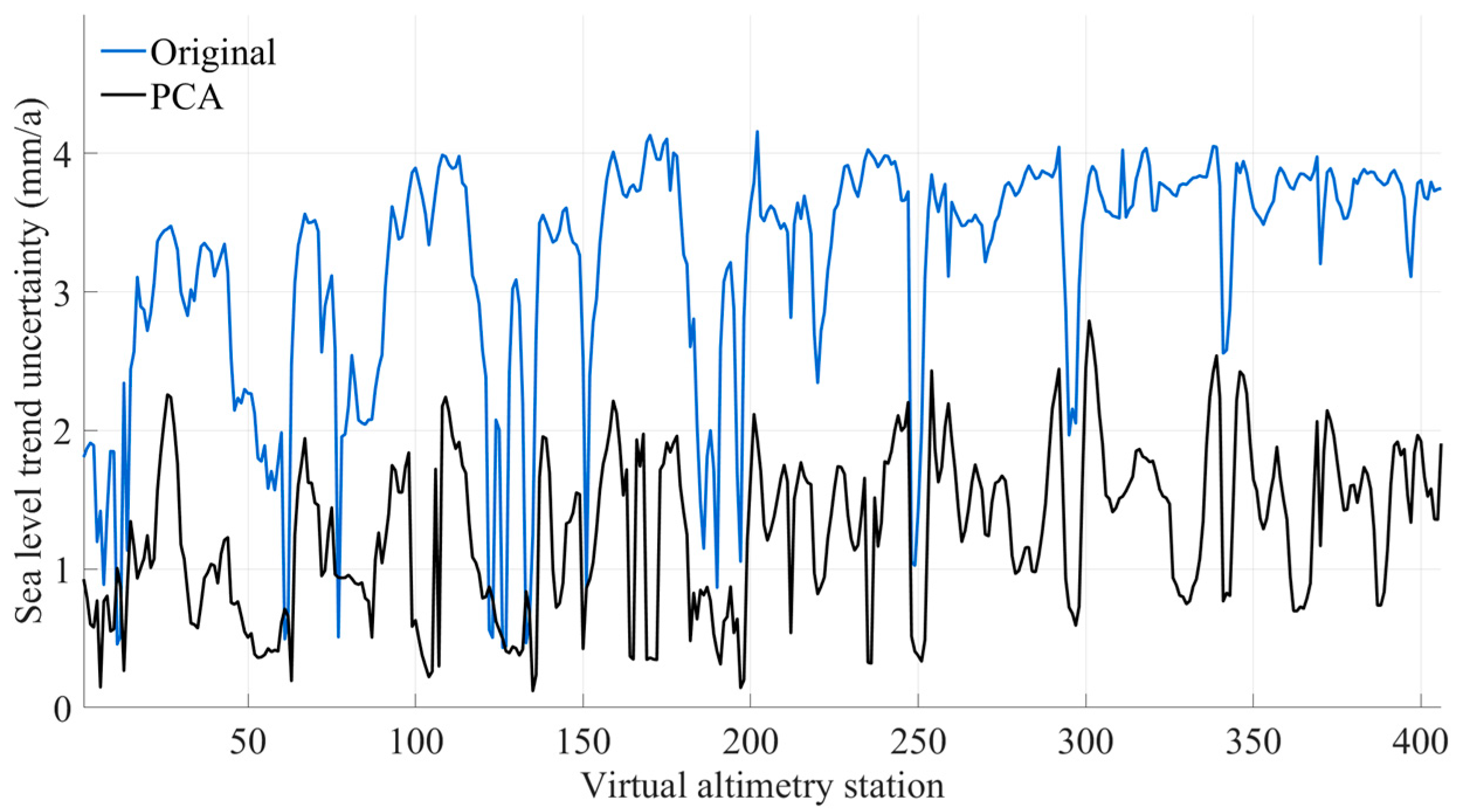

Table 1.
Sea level trends in the Black Sea across different time periods, as estimated under the optimal noise model (The number after the ± sign represents the standard deviation in this work).
Table 1.
Sea level trends in the Black Sea across different time periods, as estimated under the optimal noise model (The number after the ± sign represents the standard deviation in this work).
| This work | Existed research | |||
| Time Span(year) | Trend (mm/a) | Authors | Results (mm/a) | Time Span (year) |
| 1993-2000 | 21.68±4.05 | Cazenave et al. | 27.3±2.50 | 1993-1998 |
| 1993-2003 | 10.61±1.61 | - | - | - |
| 1993-2005 | 8.84±1.62 | Kubryakov et al. | 7.60±0.30 | 1993-2005 |
| 1993-2008 | 3.68±0.89 | - | - | - |
| 1993-2011 | 6.74±0.83 | - | - | - |
| 1993-2013 | 4.14±0.69 | Kubryakov et al. | 3.15±0.13 | 1993-2014 |
| 1993-2017 | 3.07±0.61 | Avşar et al. | 2.50±0.50 | 1993-2017 |
| 1993-2021 | 2.34±0.59 | CMEMS | 1.40±0.83 | 1993-2022 |
Table 2.
Black Sea level uncertainties in sea level trend under the optimal model (The number after the ± sign represents the standard deviation).
Table 2.
Black Sea level uncertainties in sea level trend under the optimal model (The number after the ± sign represents the standard deviation).
| Time Span (year) | Uncertainty (mm/a) |
| 1993-2000 | 12.41±3.51 |
| 1993-2003 | 8.70±2.55 |
| 1993-2005 | 7.16±2.01 |
| 1993-2008 | 5.72±1.64 |
| 1993-2011 | 5.07±1.34 |
| 1993-2013 | 4.57±1.27 |
| 1993-2017 | 3.75±1.03 |
| 1993-2021 | 3.20±0.85 |
Table 3.
Annual amplitude of sea level in the Black Sea in different time periods (The number after the ± sign represents the standard deviation).
Table 3.
Annual amplitude of sea level in the Black Sea in different time periods (The number after the ± sign represents the standard deviation).
| Time Span (year) | Annual amplitude (mm) | Uncertainty (mm) |
| 1993-2000 | 26.45±4.68 | 10.57±1.85 |
| 1993-2003 | 22.95±4.85 | 8.83±1.48 |
| 1993-2005 | 24.22±5.03 | 8.30±1.43 |
| 1993-2008 | 21.08±5.09 | 7.32±1.30 |
| 1993-2011 | 21.45±5.49 | 7.13±1.16 |
| 1993-2013 | 21.74±5.40 | 6.90±1.18 |
| 1993-2017 | 20.06±5.84 | 6.18±1.05 |
| 1993-2021 | 19.23±5.99 | 5.69±0.96 |
Table 4.
Month of maximum sea level at 406 virtual altimetry stations over the period 1993–2021.
| Month | Stations count | Percentage (%) |
| January | 3190 | 28.06 |
| February | 942 | 8.28 |
| March | 600 | 5.28 |
| April | 195 | 1.72 |
| May | 524 | 4.61 |
| June | 404 | 3.55 |
| July | 125 | 1.10 |
| August | 41 | 0.36 |
| September | 64 | 0.56 |
| October | 676 | 5.95 |
| November | 1466 | 12.90 |
| December | 3141 | 27.63 |
Table 5.
Maximum annual amplitude occurrence month for 406 virtual altimetry stations in the Black Sea over the period 1993–2021.
Table 5.
Maximum annual amplitude occurrence month for 406 virtual altimetry stations in the Black Sea over the period 1993–2021.
| Month | Stations count | Percentage (%) |
| January | 117 | 28.82 |
| February | 89 | 21.92 |
| March | 18 | 4.43 |
| April | 17 | 4.19 |
| May | 5 | 1.23 |
| June | 0 | 0.00 |
| July | 0 | 0.00 |
| August | 3 | 0.74 |
| September | 8 | 1.97 |
| October | 40 | 9.85 |
| November | 62 | 15.27 |
| December | 47 | 11.58 |
Table 6.
Comparison of estimated TG trend and annual amplitude with Literature (The number after the ± sign represents the uncertainty in this work).
Table 6.
Comparison of estimated TG trend and annual amplitude with Literature (The number after the ± sign represents the uncertainty in this work).
| Tide Gauge Station | Time Span(year) | Trend (mm/a) | Annual Amplitude (mm) | ||
| This work | References | This work | References | ||
| Poti | 1992-2001 | 7.16±0.47 | 7.01±0.12 | 156.83±3.60 | 157.76±0.05 |
| Sevastopol | 1944-1994 | 1.55±0.49 | 1.56±0.22 | 139.94±4.08 | 139.65±0.06 |
| Batumi | 1925-1996 | 3.86±0.58 | 3.52±0.15 | 157.98±3.44 | 158.48±0.06 |
| Tuapse | 1943-2011 | 2.85±0.32 | 2.92±0.14 | 136.03±4.97 | 142.41±0.06 |
| Varna | 1926-1961 | 1.35±1.46 | 1.53±0.48 | 104.23±11.78 | 152.73±0.09 |
| Constantza | 1945-1979 | 2.96±0.82 | 3.02±0.46 | 127.39±5.69 | 127.94±0.08 |
Disclaimer/Publisher’s Note: The statements, opinions and data contained in all publications are solely those of the individual author(s) and contributor(s) and not of MDPI and/or the editor(s). MDPI and/or the editor(s) disclaim responsibility for any injury to people or property resulting from any ideas, methods, instructions or products referred to in the content. |
© 2025 by the authors. Licensee MDPI, Basel, Switzerland. This article is an open access article distributed under the terms and conditions of the Creative Commons Attribution (CC BY) license (http://creativecommons.org/licenses/by/4.0/).
Copyright: This open access article is published under a Creative Commons CC BY 4.0 license, which permit the free download, distribution, and reuse, provided that the author and preprint are cited in any reuse.


