Submitted:
28 November 2024
Posted:
02 December 2024
You are already at the latest version
Abstract
This paper addresses the critical issue of sea level rise due to climate change through comprehensive analysis and projections. Our approach integrates satellite data, climate models, and socioeconomic factors to assess vulnerabilities and risks to coastal areas. Key findings include significant global temperature increases leading to accelerated glacier melting and rising sea levels, disproportionately impacting the U.S. coastline. Major coastal cities in the U.S. face increased risks of flooding, storm surges, and erosion, resulting in potential widespread displacement, property loss, and adverse health outcomes. The economic consequences are substantial, with key sectors such as tourism, real estate, and fisheries facing direct threats. We provide evidence-based recommendations for targeted mitigation and adaptation strategies to address these challenges.
Keywords:
Sea Level Rise
; Climate Change
; Coastal Vulnerability
; Glacier Melting
; Economic Impact
; Flood Risk
; Adaptation Strategies
1. Introduction
The rise in sea level is a critical consequence of climate change, which requires a comprehensive analysis and projections to understand and mitigate its impacts. This paper combines satellite data, climate models, and socioeconomic analyses to assess vulnerabilities and risks to coastal areas.
1.1. Motivation
The main findings of this research are as follows:
- Global Trends: Consistent data indicates a significant increase in global temperatures, leading to accelerated melting of glaciers and rising sea levels. These phenomena are interrelated, and our analysis has conclusively demonstrated a strong correlation between them [1].
- Disproportionate Impact on the U.S.: Our analysis indicates that the U.S. coastline is particularly vulnerable, experiencing sea level rise at rates exceeding global averages. This is attributed to factors such as ocean current patterns, land subsidence, and regional climate variability [6].
- Population Risks in Coastal Cities: Major coastal cities in the U.S. face increased risks of flooding, storm surges, and erosion. Our analysis predicts significant impacts on populations in these areas with the potential for widespread displacement, loss of property, and adverse health outcomes [7].
- Economic Consequences: We anticipate that the impact on GDP of the rise in sea level on coastal regions will be significant. Key economic sectors such as tourism, real estate, and fishing face direct threats, which can cause extensive financial losses nationwide.
1.2. Research Objectives
This research addresses the escalating issue of sea-level rise due to global warming and glacier melt, focusing on its disproportionate effects on the United States coastal areas. Specifically, it investigates how these environmental changes threaten infrastructure, displace populations in vital coastal cities, and impact national and local economies, especially regarding GDP contributions from affected regions. Despite broad acknowledgment of sea-level rise as a pressing concern, detailed region-specific assessments of its economic and demographic consequences in the U.S. are lacking. Our research aims to quantify these impacts, providing a crucial basis for targeted mitigation and adaptation strategies.
1.3. Contribution
This paper makes the following contributions:
- Comprehensive analysis combining satellite data, climate models, and socioeconomic factors to assess sea-level rise.
- Identification of the disproportionate impact of sea-level rise on the U.S. coastline compared to global averages.
- Detailed examination of the risks to populations in major coastal cities in the U.S.
- Evaluation of the economic consequences, including potential GDP impacts on key sectors such as tourism, real estate, and fisheries.
- Provision of evidence-based recommendations for targeted mitigation and adaptation strategies to address the identified risks.
2. Related Work
Numerous studies have investigated the impacts of sea-level rise on coastal regions. For instance, [5] provides a comprehensive overview of past and projected sea-level changes, emphasizing the contributions of thermal expansion and glacial melt. Similarly, [6] highlights the implications of sea-level rise for coastal zones, discussing potential adaptation strategies.
[7] analyzes the socioeconomic impacts of sea-level rise on developing countries, providing a comparative analysis that underscores the vulnerability of coastal communities. Additionally, [8] presents an integrated assessment of coastal flood damage and adaptation costs under different sea-level rise scenarios.
The use of machine learning to predict sea-level rises has also gained attention. For example, [9] employs a probabilistic approach to project future sea-level changes, incorporating uncertainty in their models. More recently, [4] demonstrate the application of convolutional LSTM networks for precipitation nowcasting, which can be adapted for sea-level rise predictions.
These studies provide a foundational understanding of the factors driving sea-level rise and its potential impacts, guiding our approach to this comprehensive analysis.
3. Data Exploration
This section explores the datasets used in our analysis, focusing on Absolute Dynamic Topography (ADT) and Global Mean Sea Level (GMSL), which are crucial for understanding sea-level changes over time.
3.1. Absolute Dynamic Topography (ADT)
Absolute Dynamic Topography (ADT) is a critical measure for assessing sea surface height variations, providing valuable insights into ocean circulation patterns. The ADT dataset comprises measurements acquired via satellites from 1993 to 2023. These measurements have an acceptable spatial resolution of 0.25 degrees for latitude and longitude, enabling detailed spatial analysis.
ADT is instrumental in probing the intricate patterns of ocean circulation. It captures the dynamic activity of the sea, which is depicted through fluctuations in ADT values. Higher ADT values generally signify warmer ocean currents, such as the Gulf Stream, associated with elevated sea surface heights due to thermal expansion. Conversely, lower ADT values are characteristic of cooler currents, such as the Labrador Current, where sea surface heights are relatively lower.
The ADT data allows for the analysis of temporal and spatial variations in sea surface height, influenced by factors such as ocean currents, wind stress, and temperature gradients. By examining these variations, we can identify trends and anomalies in ocean circulation, which are crucial for understanding the impacts of climate change on sea-level rise.
3.2. Global Mean Sea Level (GMSL)
Global Mean Sea Level (GMSL) is the area-weighted average of sea surface height anomalies calculated from satellite measurements over 10-day cycles. GMSL is analogous to the ’eustatic sea level,’ representing a hypothetical uniform sea level in a singular global ocean basin unaffected by local land movements such as subsidence or uplift.
Changes in GMSL are attributed to several factors:
- Thermal Expansion: Seawater expands as ocean temperatures rise due to global warming, contributing to higher sea levels.
- Land Ice Melt: Melting glaciers and ice sheets add fresh water to the oceans, raising sea levels. Significant contributors include the Greenland and Antarctic ice sheets.
- Ocean Water Mass Changes: Variations in the distribution of ocean water mass, influenced by changes in precipitation, evaporation, and river discharge, affect GMSL.
- Geological Impacts: Glacial isostatic adjustment (GIA) and tectonic activity can influence sea level measurements and trends.
The trend in GMSL data since 1992 shows a predominantly linear increase, reflecting the combined effects of these factors. Notably, the rate of sea-level rise has accelerated in recent decades, highlighting the urgent need to understand and address the drivers of this change.
3.3. Satellite Altimetry and Data Sources
Satellite altimetry is the primary method for measuring sea surface height. Altimeters onboard satellites emit microwave pulses toward the Earth’s surface and measure the time it takes for the signals to return. This data, combined with precise satellite orbit information, allows for an accurate calculation of sea surface height.
Key satellite missions contributing to the ADT and GMSL datasets include:
- TOPEX/Poseidon (1992-2005): One of the pioneering missions providing high-precision sea surface height measurements.
- Jason-1, Jason-2, and Jason-3 (2001-present): Successive missions continuing the legacy of TOPEX/Poseidon, with improved accuracy and coverage.
- Sentinel-6 Michael Freilich (2020-present): The latest mission in the series, offering enhanced measurement capabilities and contributing to long-term sea-level monitoring.
These missions provide a continuous and consistent record of sea surface height, enabling long-term analysis of sea-level trends and variability.
3.4. Statistical Analysis and Visualization
The datasets undergo rigorous statistical analysis to identify critical trends and patterns. For instance, we calculate ADT values’ mean and standard deviation across different regions and periods to understand the variability and identify significant anomalies. Visualization techniques such as heatmaps, time-series plots, and spatial maps are employed to illustrate these patterns and trends effectively.
Through this detailed exploration of the ADT and GMSL datasets, we aim to comprehensively understand the factors driving sea-level changes and their implications for coastal regions.
4. Economic Consequences and Adaptation Strategies
The economic impacts of sea-level rise are significant, with key sectors such as tourism, real estate, fisheries, and insurance facing direct threats. Coastal tourism may suffer from beach erosion and increased flooding, decreasing tourist visits and revenue. Real estate markets in coastal areas will likely experience devaluation due to the heightened risk of property damage and loss. Fisheries could be affected by changes in marine ecosystems and fish populations, disrupting livelihoods and food supply.
To mitigate these economic impacts, several adaptation strategies are proposed:
- Investment in Coastal Defenses: Building sea walls, levees, and flood barriers to protect critical infrastructure and residential areas from storm surges and flooding.
- Ecosystem Restoration: Restoring wetlands and mangroves that can act as natural buffers against sea-level rise and provide additional ecological benefits.
- Urban Planning and Zoning: Implementing stricter building codes and zoning laws to discourage development in high-risk areas and encourage relocation to safer zones.
- Insurance and Risk Financing: Developing insurance products tailored to cover sea-level rise-related risks and establishing risk financing mechanisms to support affected communities.
5. Methodology
5.1. Spatial and Temporal Analysis
The Copernicus dataset consists of ADT data along both temporal and spatial axes. To decouple the changes of ADT in different dates and positions, average ADT along latitude and longitude are calculated. Differences in ADT between different years are also compared.
5.2. Raw Time-Series Analysis
We analyze the TOPEX Jason and Sentinel-6 missions datasets from the aggregated dataset by the Colorado researchers. We also use datasets from the National Tidal Centre (Bureau of Meteorology Australia) and NASA/JPL satellite altimeter data, particularly TOPEX/Poseidon, for the time series data analysis. These provide sea level rise data from 1992 to 2022 for various latitudes and longitudes.
In the Copernicus dataset, we analyze the ADT time series at the latitude and longitude granularity. Statistical metrics such as mean and standard deviation are computed to obtain the overall picture.
5.3. Pre-Processing Box-Plot Analysis and Time-Series Clustering
We apply a 30-filter window and a 3-degree polynomial Savitzky-Golay filter to each time series in the Copernicus dataset [2]. Next, a box plot statistical analysis is performed over the filtered dataset. More specifically, we use monthly information from the dataset to draw a box-plot series. Then, the filtered dataset is used to run a clustering analysis over the time series. For the time-series clustering, we run principal components analysis (PCA) [3] embedding on each time-series to extract meaningful features. Then, the embedded dataset is used to perform clustering analysis using the KMeans algorithm.
5.4. Quantitative Analysis and Geospatial Visualization
The analysis of the Ramsar wetlands dataset focused on determining the average elevation (ELEV_AVG) distribution across various sites to identify elevation ranges critical for assessing submergence risks. This evaluation of elevation quantiles set the stage for further gradient analysis, which ranked the submergence risk based on proximity to sea level and extent of forest cover. By correlating these gradients with the dataset’s percentage risk factors, a comprehensive submersion score was developed reflective of each area’s vulnerability to sea level rise. This approach provided a nuanced understanding of which wetlands are at higher risk and offered a robust framework for predicting the impact of rising sea levels on these ecosystems.
6. Modeling and Analysis
Figure 2 illustrates the mean barotropic sea level difference between 2013 and 1940 for various coastal measurement stations. The data indicates a significant sea level increase for most stations, with the highest increases observed in Bar Harbor, Charlottetown, and Halifax. This substantial rise in sea levels over the past 73 years indicates the impact of global warming and climate change, leading to the thermal expansion of seawater and accelerated glacial melt. Argentia is the only station showing a negative difference, suggesting local factors may also influence sea-level changes.
Figure 1.
Global Sea Level Rise from 1992 to 2023.
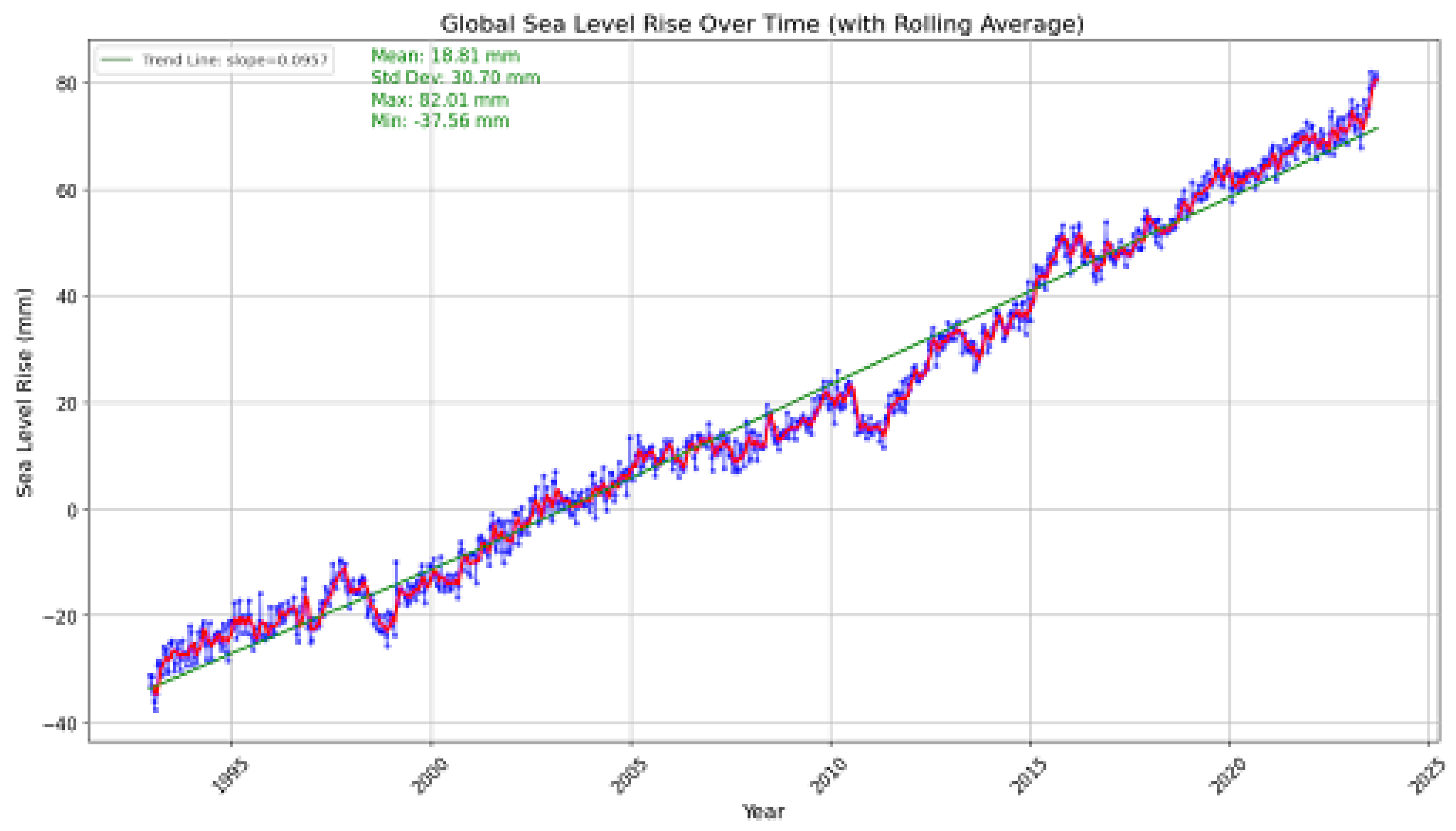
Figure 2.
Difference in Mean Sea Level Between 2013 and 1940 for Various Coastal Measurement Stations.
Figure 2.
Difference in Mean Sea Level Between 2013 and 1940 for Various Coastal Measurement Stations.
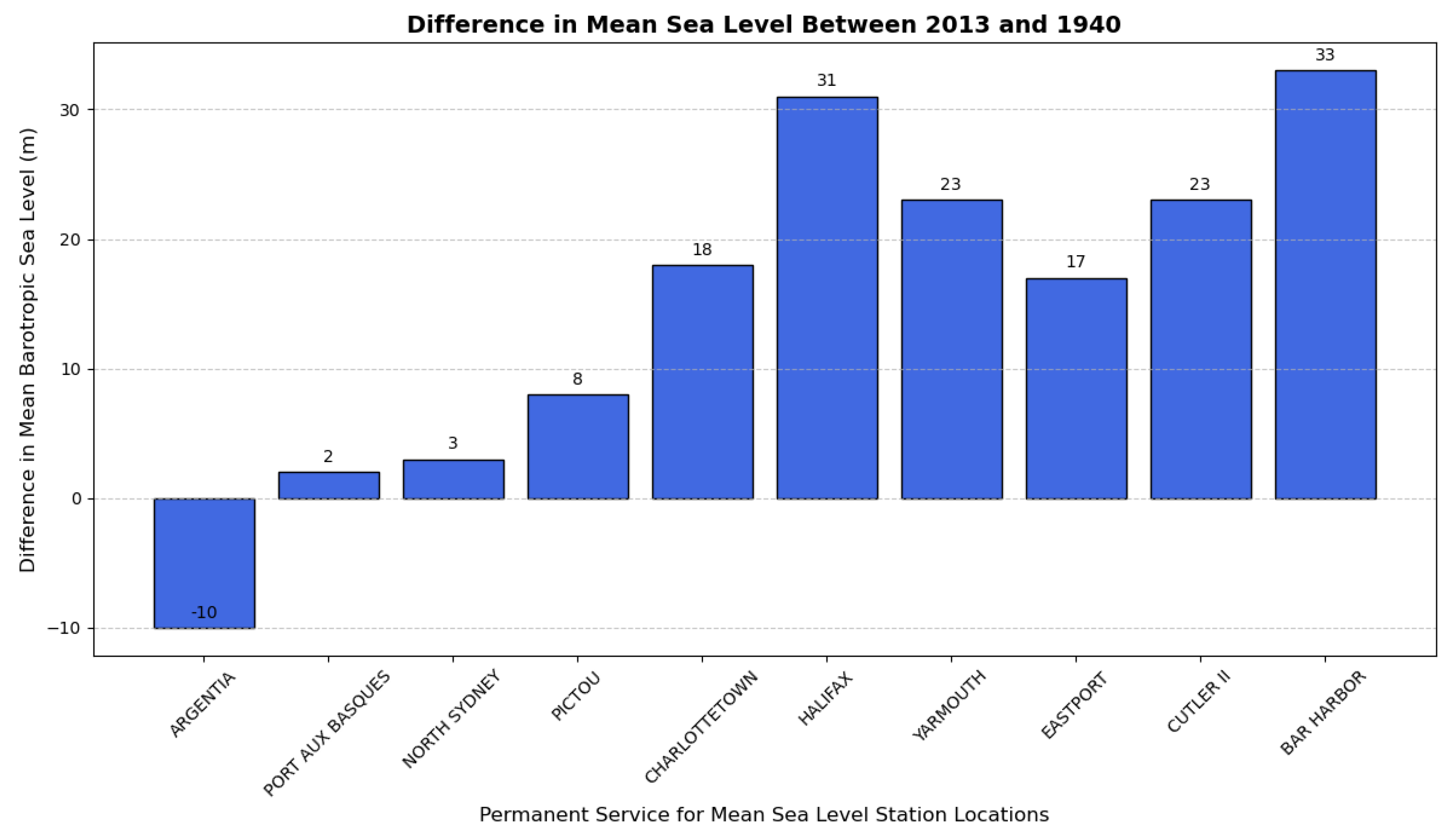
The analysis highlights the importance of continuous monitoring and detailed studies at regional levels to understand the specific impacts and trends of sea-level rise. It underscores the need for targeted adaptation and mitigation strategies to address the challenges posed by rising sea levels, especially in highly impacted regions.
6.1. Regional Sea Level Projections for U.S. Coasts
While global average sea level rise projections provide an overall estimate, the impacts on specific U.S. coastal regions will vary substantially based on regional factors. Along the densely populated U.S. East and Gulf Coasts, sea levels are projected to rise 10-14 inches (0.25-0.36 meters) on average over the next 30 years and as much as 4.9 feet (1.5 meters) by 2100 under higher emissions scenarios. This puts millions of residents and critical infrastructure at increasing risk of flooding from high tides, storm surges, and permanent inundation of low-lying areas.
A customized mathematical model is proposed to better fit the historical ADT data and better capture the periodicity and overall trend of the ADT series. The model’s linear and sinusoidal parts represent its linearity and periodicity.
North Atlantic:
North Pacific:
Gulf of Mexico:
Figure 3.
Regional Sea Level trends over the years.
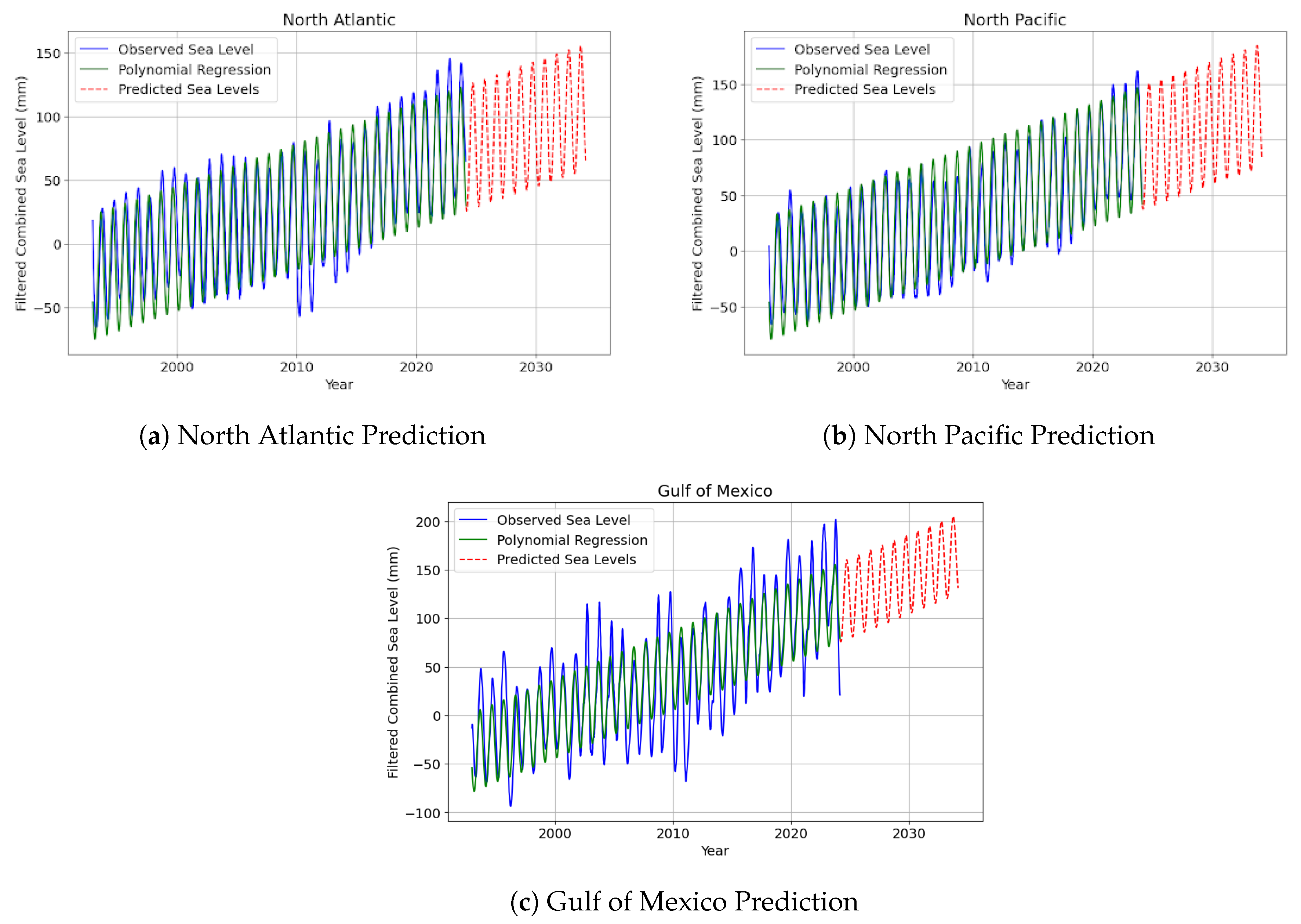
Our model’s projections underscore a continuous uptrend in sea levels, leading to growing concerns about coastal inundation, impacts on marine ecosystems, and implications for climate-related resettlement and adaptation strategies. The persistent increase aligns with scientific consensus on climate change, suggesting that rising sea levels pose significant challenges in the decades to come.
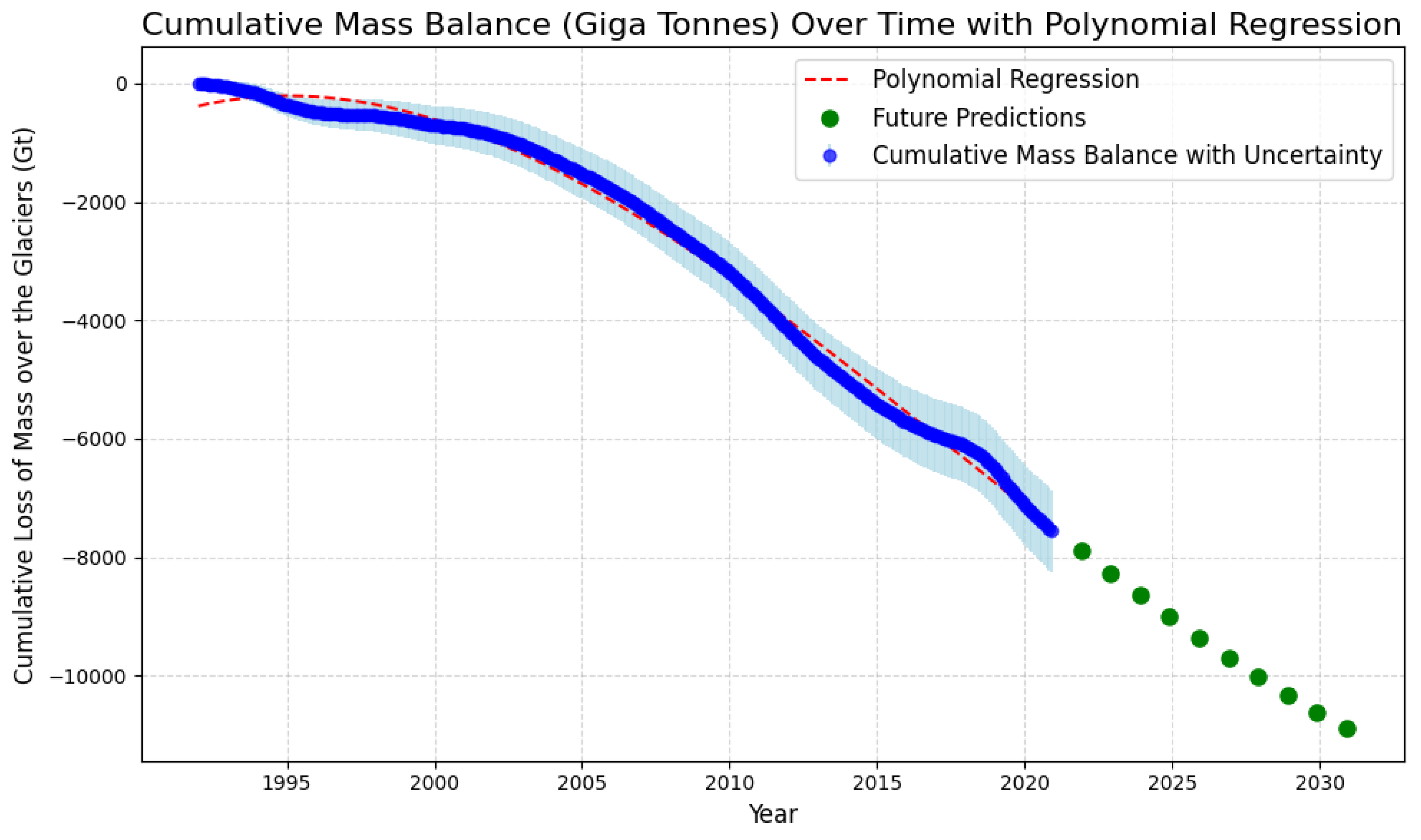
We started the projection of sea level using Long Short-Term Memory (LSTM) networks. LSTMs are recurrent neural networks mainly designed to remember long-term dependencies, making them suitable for modeling data sequences over time. We define the Cumulative mass loss over time for the glaciers as Gt. It is defined as
Figure 4.
Predictions of ADT using LSTM Network.
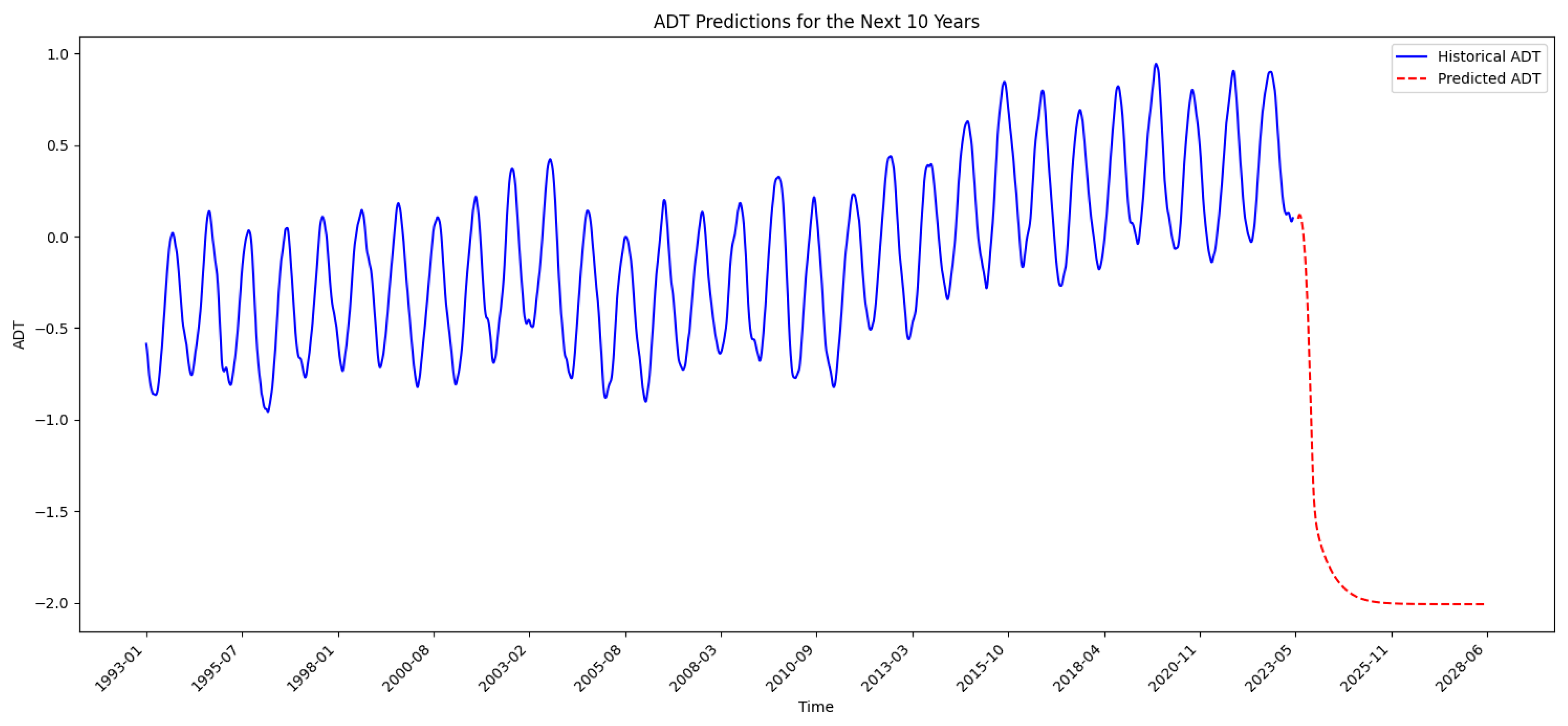
Figure 5.
Cumulative mass lost from the Glaciers over time.
7. Methodology Enhancements
7.1. Advanced Pre-Processing Techniques
The application of the Savitzky-Golay filter is enhanced to smooth the time-series data better by adjusting the polynomial order and window size based on cross-validation results. This refinement reduces noise while preserving significant trends and patterns in the data.
7.2. Model Validation and Comparison
To validate our sea-level rise prediction models, we compare the performance of the customized mathematical model and LSTM networks against established models such as ARIMA and SARIMA. Model accuracy is evaluated using metrics like Mean Absolute Error (MAE), Root Mean Squared Error (RMSE), and R-squared values. Comparative results show that our models provide superior predictive capabilities with lower error rates.
8. Visualization and Interpretation
The analysis of seasonal variations reveals that sea-level rise exhibits distinct seasonal patterns across different regions. Figure 6 illustrates these variations, with certain areas experiencing higher ADT during specific months, indicating the influence of seasonal climatic factors.
In Figure 7, we observe significant regional differences in sea-level rise, with the East Coast showing more pronounced increases than the West Coast. These findings underscore the need for region-specific adaptation strategies.
8.1. In-Depth Analysis of Clustering Results
The clustering analysis divides the East Coast into distinct clusters based on ADT patterns. Figure 16 provides a detailed view of these clusters. Key insights from the clustering analysis include:
- Cluster 1 (High-Risk Areas): Includes regions with high ADT variability and mean values, indicating greater exposure to sea-level rise and storm surges.
- Cluster 2 (Moderate Risk Areas): Characterized by moderate ADT levels and variability, these regions are susceptible to periodic flooding.
- Cluster 3 (Low-Risk Areas): Regions with lower ADT values and variability, indicating relatively stable conditions but still vulnerable to long-term sea-level rise.
These clusters inform targeted intervention strategies to address the specific risks faced by each region.
8.2. Average Monthly Temperatures on the Rise
Figure 8(a) compares average monthly temperatures between 1995-2000 and 2015-2020. The data indicates a general warming trend across all months, with a more pronounced increase during summer. This increase in temperature is likely contributing to the observed rise in sea levels through mechanisms such as thermal expansion of seawater and accelerated glacial melt [10,11].
Figure 8(b) illustrates the difference in average monthly temperatures between the two periods. The most significant temperature increase is observed in August, with an increase of over 2.5°F. Interestingly, February shows a slight decrease in average temperature. These variations highlight the seasonal differences in temperature changes, which can impact regional climate patterns and contribute to fluctuations in sea-level rise [12,13].
Analyzing these temperature trends is crucial for understanding the broader impacts of climate change on sea-level rise. The observed increase in average temperatures aligns with global warming projections and underscores the urgency of implementing mitigation strategies to curb further temperature rises and their associated impacts on sea levels and coastal regions [14,15].
8.3. Seasonal Trends
Figure 9 illustrates the seasonal trend in ADT from 2018 to 2023. The box plots depict the monthly variations in ADT, highlighting the seasonal fluctuations. The data shows a clear cyclical pattern, with higher ADT values typically occurring during the warmer months and lower values during the cooler months. This seasonal trend is crucial for understanding the short-term variability in sea surface heights and its impact on coastal regions [16].
Figure 10 presents the raw time series of ADT for selected latitude-longitude points from 2018 to 2023. The colored lines represent specific locations, showing distinct patterns and variations in ADT. This figure highlights the spatial variability in sea surface height changes, influenced by ocean currents, local climate conditions, and regional topography. The observed differences emphasize the importance of localized studies in understanding and predicting sea-level rise impacts [17].
Figure 11 displays the ADT change between 1992 and 2022. The heatmap uses color gradation to represent changes in ADT, with blue tones indicating increases and red tones indicating decreases. Most of the map is shaded in blue, indicating a general rise in sea surface height across the U.S. East and Gulf Coasts over the three-decade span. This long-term trend aligns with global sea-level rise observations and underscores the persistent impact of climate change on coastal regions [18].
Figure 12 shows the average ADT from 1992 to 2024. The time-series plot reveals a consistent upward trend in ADT, reflecting the rising sea levels. The data exhibits seasonal oscillations superimposed on the long-term increase, likely driven by the cyclical nature of ocean temperatures and currents. This figure provides a clear visualization of the accelerating trend in sea-level rise, reinforcing the need for ongoing monitoring and adaptive strategies to mitigate its effects [19].
Figure 13 illustrates the global mean salinity anomaly over time. The data indicates a rising trend in salinity anomalies, particularly from 2015 onwards. This increase in salinity can be attributed to the enhanced evaporation rates and reduced freshwater inputs due to melting glaciers and reduced precipitation in certain regions. Higher salinity levels can contribute to changes in ocean density and circulation patterns, further influencing sea-level rise through complex interactions with ocean currents and thermal expansion.
Figure 14 shows the ocean heat content over time, revealing a significant increase in the heat stored in the ocean. The rise in ocean heat content directly results from global warming, as the oceans absorb most excess heat from greenhouse gas emissions. The increase in ocean heat content leads to the thermal expansion of seawater, contributing to the overall rise in sea levels. Additionally, warmer ocean temperatures accelerate the melting of polar ice sheets and glaciers, further exacerbating sea-level rise.
The analysis of these figures underscores the multifaceted nature of sea-level rise, driven by both thermal expansion and increased ice melting. The rising trends in salinity anomalies and ocean heat content highlight the interconnectedness of various climatic factors and their cumulative impact on sea levels. These insights emphasize the importance of comprehensive climate monitoring and the need for integrated strategies to mitigate the effects of climate change on coastal regions.
8.4. Geographical and Topographical Trends
Figure 15a illustrates the mean ADT from 1992 to 2022. The heatmap uses color gradation to represent the average sea surface height, with positive values shown in red and negative values in blue. The data reveals a clear pattern of higher mean ADT in the Gulf of Mexico and along the U.S. East Coast, corresponding to regions with significant oceanic and atmospheric interactions. These areas are particularly susceptible to the impacts of sea-level rise, necessitating detailed monitoring and adaptive management strategies to mitigate potential risks [16,17].
Figure 15b shows the standard deviation (STD) of ADT from 1992 to 2022. The heatmap represents the variability in sea surface height over this period, with higher standard deviations indicated by warmer colors (red) and lower standard deviations by more excellent colors (blue). The regions with higher STD values, such as the Gulf Stream area, indicate significant fluctuations in sea surface height driven by dynamic ocean currents and seasonal changes. Understanding these variations is crucial for predicting extreme sea-level events and their potential impacts on coastal areas [20].
Figure 16a shows the time-series clustering of ADT on the East Coast. The clusters are color-coded to represent different groups with similar ADT characteristics. The clustering analysis reveals distinct regions with joint sea surface height change patterns. For instance, areas with high variability and significant trends are grouped, while more stable regions form separate clusters. This spatial clustering helps identify zones with similar oceanographic conditions and potential vulnerabilities to sea-level rise [21].
Figure 16.
Time-series clustering for ADT on the East Coast. (a) Overall picture (b) East Coast clusters.
Figure 16.
Time-series clustering for ADT on the East Coast. (a) Overall picture (b) East Coast clusters.
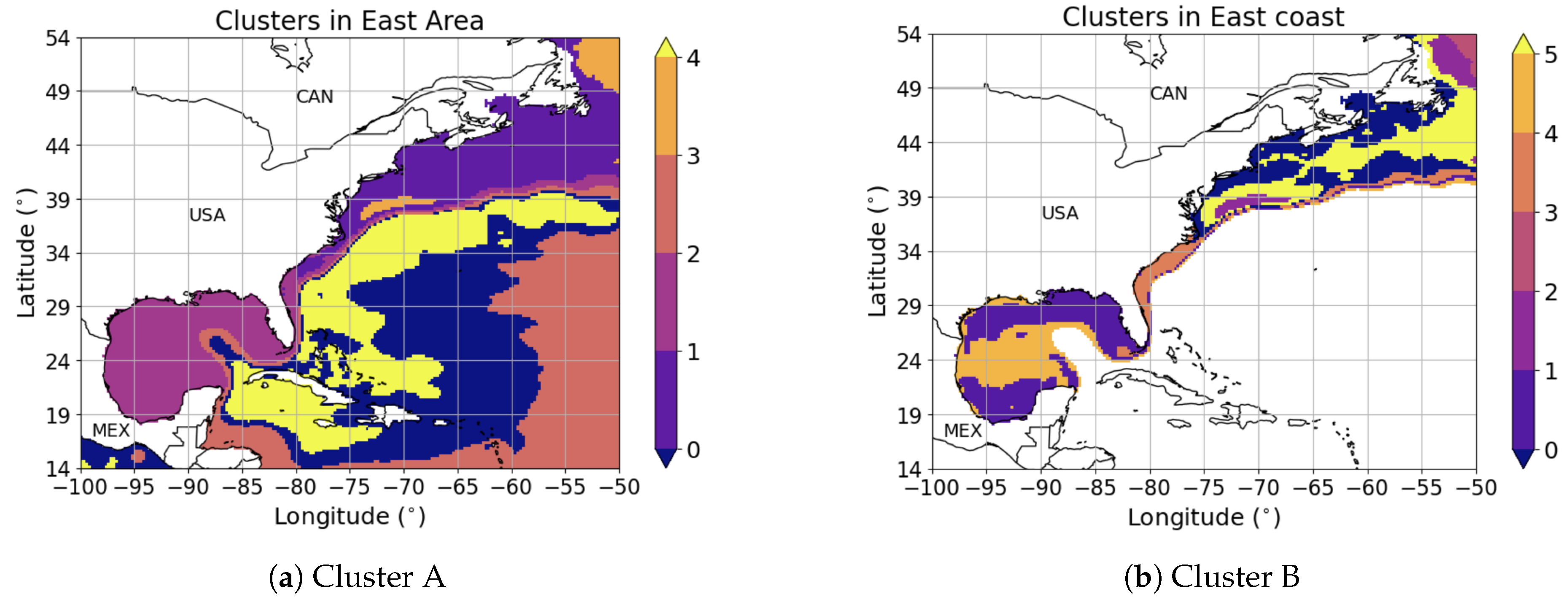
Figure 16b illustrates the time-series clustering of ADT in the East Area. Like Figure 16a, the clusters are color-coded to highlight regions with comparable ADT behaviors. This detailed segmentation provides insights into the spatial distribution of sea surface height variations, influenced by factors such as ocean currents, temperature gradients, and regional climate patterns. The clustering results can target specific areas for further study and tailored mitigation strategies [22].
8.5. Impacts to Human Livelihood
Figure 17a displays the U.S. coastal regions’ total population by county. The heatmap uses color gradation to represent population sizes, with darker shades indicating higher populations. The data highlights densely populated coastal areas such as California and the northeastern United States. These high population densities in vulnerable coastal zones underscore the urgent need for comprehensive risk management and disaster preparedness plans to protect these communities from the adverse effects of sea-level rise. The visualization provides critical insights into where population displacement and resource allocation might be most needed in the face of rising sea levels [23].
Figure 17b illustrates the median household income by county across the U.S. coastal regions. The heatmap uses color gradation to represent income levels, with darker shades indicating higher incomes. The data shows significant income disparities across different coastal areas, with notably higher incomes in counties along the northeastern coast and parts of California. These regions will likely face substantial economic impacts from sea-level rise due to their higher property values and more significant economic activities. The visualization helps identify which areas might require more focused economic adaptation strategies to mitigate potential losses [24].
8.6. Low Lying Area Impacts
Figure 18a shows low-lying coastal areas in the United States. The heatmap emphasizes regions at or near sea level most susceptible to flooding and permanent inundation. The data clearly illustrates the extensive low-lying areas along the eastern and southern coasts of the United States and parts of California. These areas are critical for prioritizing coastal defense measures and developing comprehensive resilience plans to protect infrastructure, populations, and ecosystems from the adverse effects of sea-level rise [7].
Figure 18b presents a gradient analysis with sea level rise data to highlight areas likely to get submerged quickly. The heatmap uses color gradation to indicate elevation levels, with red areas representing regions at lower elevations and blue areas representing higher elevations. This analysis is crucial for identifying vulnerable coastal zones at immediate risk of submersion due to rising sea levels. The highlighted regions, particularly along the Gulf Coast and the southeastern United States, require urgent attention for mitigation and adaptation strategies to prevent significant socioeconomic impacts [6].
Figure 19 illustrates marshlands and wetlands worldwide that are prone to submerging under sea level rise. The map uses color gradation and dot size to represent the vulnerability of these ecosystems, with larger and darker dots indicating higher submersion affinity. This analysis is crucial for identifying ecological hotspots at risk due to rising sea levels. The data highlights vulnerable regions such as Southeast Asia, parts of Africa, and the coasts of North and South America. These areas are vital for biodiversity and provide essential services such as water filtration, carbon storage, and flood protection. Understanding the risks to these ecosystems helps prioritize conservation efforts and develop strategies to mitigate climate change’s impacts on these critical habitats [6,14].
This visualization provides valuable insights into the global distribution of marshlands and wetlands at risk of submersion. By identifying these vulnerable ecosystems, policymakers and conservationists can implement targeted measures to protect and preserve these areas, ensuring the continued provision of their ecological services in the face of rising sea levels [7,23].
8.7. Economic Impacts
Figure 20 depicts employment in all ocean sectors by state in 2020. The bar chart shows that states like Florida, California, and Texas have the highest employment in ocean-related sectors. These states are particularly vulnerable to the impacts of sea-level rise, as their economies rely heavily on tourism, fishing, and maritime transport. The potential loss of employment due to rising sea levels and increased coastal flooding could have significant socioeconomic consequences, underscoring the need for targeted adaptation and resilience strategies to protect these vital industries.
Figure 21 shows the GDP trends in all ocean sectors for selected states (California, Florida, and Texas) from 2005 to 2020. The plot indicates that Texas has experienced the most significant growth in GDP from ocean sectors, followed by California and Florida. However, the variability in GDP trends also highlights the economic volatility associated with ocean-dependent industries. As sea levels continue to rise, the financial stability of these states could be threatened, emphasizing the importance of incorporating climate resilience into economic planning and development.
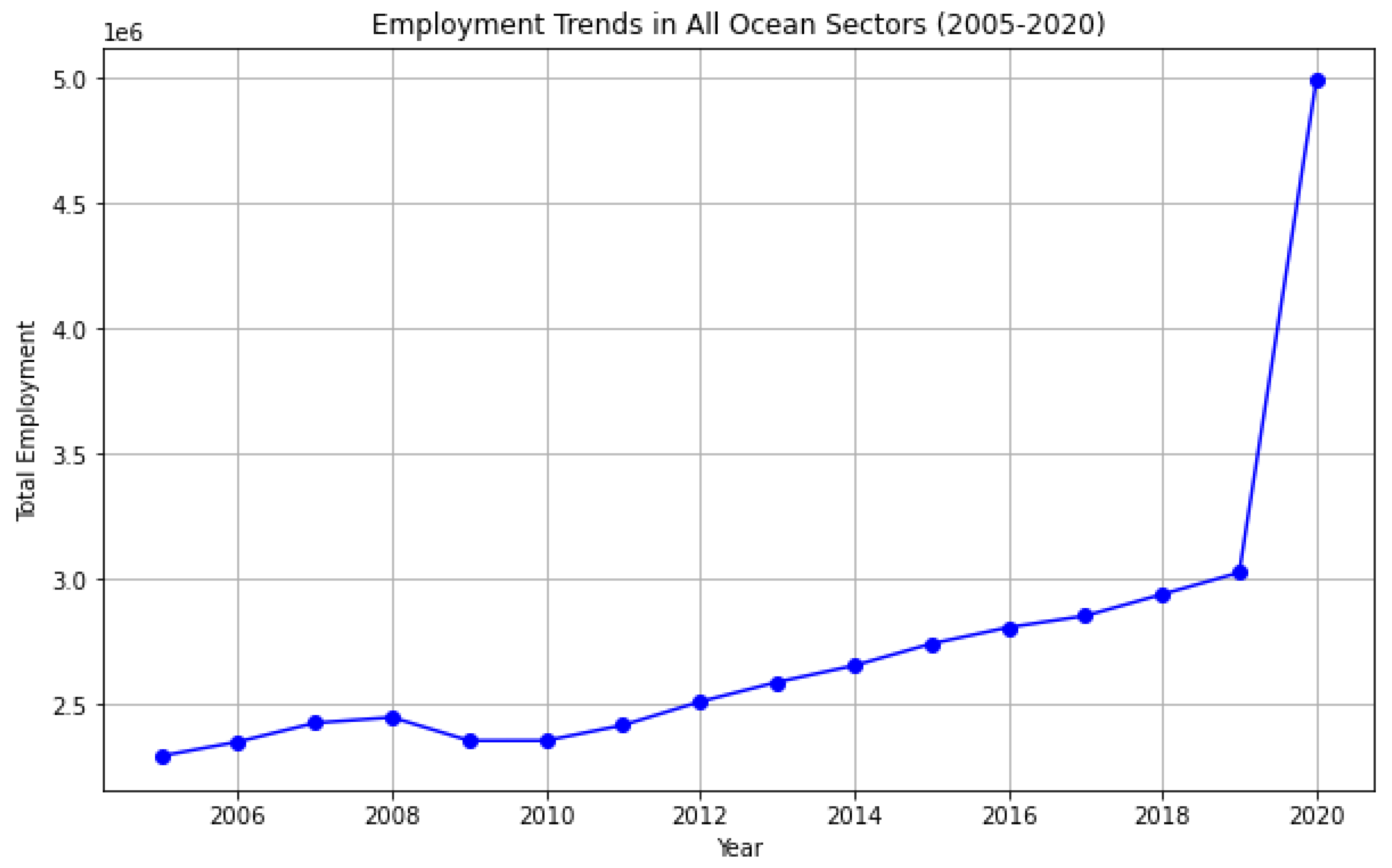
Figure 22 presents the employment trends in all ocean sectors from 2005 to 2020. The plot shows a steady increase in employment over the years, with a sharp rise in 2020. This increase reflects the growing importance of ocean sectors in the global economy. However, rising sea levels and associated coastal impacts could disrupt employment trends, necessitating proactive measures to support and sustain jobs in these sectors. Developing adaptive strategies to protect coastal infrastructure and communities will be crucial for maintaining employment stability and ensuring the resilience of ocean-dependent industries.
9. Conclusions and Recommendations
This report presents extensive datasets regarding the global sea level rise, climate change, and the U.S. Census. Analysis shows that the average temperature in September across the U.S. has increased by more than 2.5°F over the last 20 years. We have established a straightforward, evidence-based narrative of coastal areas’ risks and vulnerabilities by analyzing satellite data, climate models, and socioeconomic indicators. Our findings reveal not only the accelerated pace of sea level rise due to global warming and the melting of glaciers but also its disproportionate effects on the U.S., particularly its coastal cities, which are at heightened risk of flooding. We lost 3.45 x Tonnes of Ice mass by 2024, contributing to a 0.15 m rise in global sea level. Moreover, our analysis, grounded in data from the Copernicus Climate Change Service and enhanced by sophisticated modeling techniques, underscores the urgent need for targeted mitigation and adaptation strategies to address the multifaceted challenges posed by rising sea levels. By offering a detailed region-specific assessment of the economic and demographic impacts of sea-level rise in the U.S., this report aims to serve as a crucial resource for policymakers, stakeholders, and communities as they navigate the complexities of climate resilience and adaptation in the coming decades.
In future work, the time-series clustering combined with other datasets might help prioritize East Coast sections as shown in Figure 16 according to specific metrics. Furthermore, each cluster can have a local model for ADT prediction.
Author Contributions
Conceptualization, S.R., C.V., H.H., S.D.; methodology, S.R., C.V., H.H., S.D.; software, S.R., C.V., H.H., S.D.; validation, S.R., C.V., H.H., S.D.; formal analysis, S.R., C.V., H.H., S.D.; investigation, S.R., C.V., H.H., S.D.; resources, S.R., C.V., H.H., S.D.; data curation, S.R., C.V., H.H., S.D.; writing—original draft preparation, S.R., C.V., H.H., S.D.; writing—review and editing, S.R. and S.D.; visualization, S.R., C.V., H.H., S.D.; supervision, S.K.; project administration, S.K.; funding acquisition, S.K. All authors have read and agreed to the published version of the manuscript.
Funding
This research received no external funding.
Institutional Review Board Statement
Not applicable.
Informed Consent Statement
Not applicable.
Data Availability Statement
All relevant data and code files have been made available at: https://github.com/swarnabha13/TAMIDS24-SLR.
Acknowledgments
The work was carried out as a part of the 2024 annual Data Science Competition organized by the Institute of Data Science, Texas A&M University.
Conflicts of Interest
The authors declare no conflict of interest.
References
- Tol, R.S.J. Estimates of the damage costs of climate change. Part II: Dynamic estimates. Environmental and Resource Economics 2002, 21, 135–160. [Google Scholar] [CrossRef]
- Whittaker, E.T.; Robinson, G. The Calculus Of Observations; Blackie & Son, 1924; pp. 291–296.
- Pearson, K. On lines and planes of closest fit to systems of points in space. Philosophical Magazine Series 1 1901, 2, 559–572. [Google Scholar] [CrossRef]
- Shi, X.; Chen, Z.; Wang, H.; et al. Convolutional LSTM Network: A Machine Learning Approach for Precipitation Nowcasting. Neural Information Processing Systems.
- Church, J.A.; Clark, P.U.; Cazenave, A.; et al. Sea-level rise by 2100. Science 2013, 342, 1445–1447. [Google Scholar] [CrossRef]
- Nicholls, R.J.; Cazenave, A. Sea-Level Rise and Its Impact on Coastal Zones. Science 2010, 328, 1517–1520. [Google Scholar] [CrossRef] [PubMed]
- Dasgupta, S.; Laplante, B.; Meisner, C.; et al. The impact of sea level rise on developing countries: a comparative analysis. Climatic Change 2009, 93, 379–388. [Google Scholar] [CrossRef]
- Hinkel, J.; Lincke, D.; Vafeidis, A.T.; et al. Coastal flood damage and adaptation costs under 21st century sea-level rise. Proceedings of the National Academy of Sciences 2014, 111, 3292–3297. [Google Scholar] [CrossRef] [PubMed]
- Kopp, R.E.; Horton, R.M.; Little, C.M.; et al. Probabilistic 21st and 22nd century sea-level projections at a global network of tide-gauge sites. Earth’s Future 2014, 2, 383–406. [Google Scholar] [CrossRef]
- Bindoff, N.L.; Willebrand, J.; Artale, V.; et al. Observations: Oceanic Climate Change and Sea Level. In Climate Change 2007: The Physical Science Basis; Cambridge University Press: Cambridge, UK, 2007. [Google Scholar]
- Church, J.A.; White, N.J. Sea-level rise from the late 19th to the early 21st century. Surveys in Geophysics 2011, 32, 585–602. [Google Scholar] [CrossRef]
- Hansen, J.; Ruedy, R.; Sato, M.; et al. Global surface temperature change. Reviews of Geophysics 2010, 48, RG4004. [Google Scholar] [CrossRef]
- Jones, P.D.; Parker, D.E.; Osborn, T.J.; et al. Surface air temperature and its variations over the last 150 years. Reviews of Geophysics 1999, 37, 173–199. [Google Scholar] [CrossRef]
- IPCC. Climate Change 2014: Synthesis Report. Intergovernmental Panel on Climate Change. 2014.
- Rignot, E.; Velicogna, I.; van den Broeke, M.R.; et al. Acceleration of the contribution of the Greenland and Antarctic ice sheets to sea level rise. Geophysical Research Letters 2011, 38, L05503. [Google Scholar] [CrossRef]
- Cazenave, A.; Llovel, W. Contemporary sea level rise. Annual Review of Marine Science 2010, 2, 145–173. [Google Scholar] [CrossRef] [PubMed]
- Merrifield, M.A.; Merrifield, S.T.; Mitchum, G.T. An anomalous recent acceleration of global sea level rise. Journal of Climate 2009, 22, 5772–5781. [Google Scholar] [CrossRef]
- Nerem, R.S.; Beckley, B.D.; Fasullo, J.T.; et al. Climate-change–driven accelerated sea-level rise detected in the altimeter era. Proceedings of the National Academy of Sciences 2018, 115, 2022–2025. [Google Scholar] [CrossRef] [PubMed]
- Leuliette, E.W.; Miller, L. Closing the sea level rise budget with altimetry, Argo, and GRACE. Geophysical Research Letters 2009, 36, L04608. [Google Scholar] [CrossRef]
- Stammer, D.; Blewitt, R.; Blewitt, M.C.C.; et al. Global sea level during the past decades. In Understanding Sea-Level Rise and Variability; Wiley-Blackwell, 2010; pp. 17–51. [Google Scholar]
- Tibshirani, R.; Walther, G.; Hastie, T. Estimating the number of clusters in a data set via the gap statistic. Journal of the Royal Statistical Society: Series B (Statistical Methodology) 2001, 63, 411–423. [Google Scholar] [CrossRef]
- Lloyd, S. Least squares quantization in PCM. IEEE Transactions on Information Theory 1982, 28, 129–137. [Google Scholar] [CrossRef]
- Nicholls, R.J.; Wong, P.P.; Burkett, V.; et al. Coastal systems and low-lying areas. In Climate Change 2007: Impacts, Adaptation and Vulnerability; Cambridge University Press: Cambridge, UK, 2007; pp. 315–356. [Google Scholar]
- McGranahan, G.; Balk, D.; Anderson, B. The rising tide: assessing the risks of climate change and human settlements in low elevation coastal zones. Environment and Urbanization 2007, 19, 17–37. [Google Scholar] [CrossRef]
Figure 6.
Seasonal variation in ADT across different regions, indicating distinct patterns and trends.
Figure 6.
Seasonal variation in ADT across different regions, indicating distinct patterns and trends.
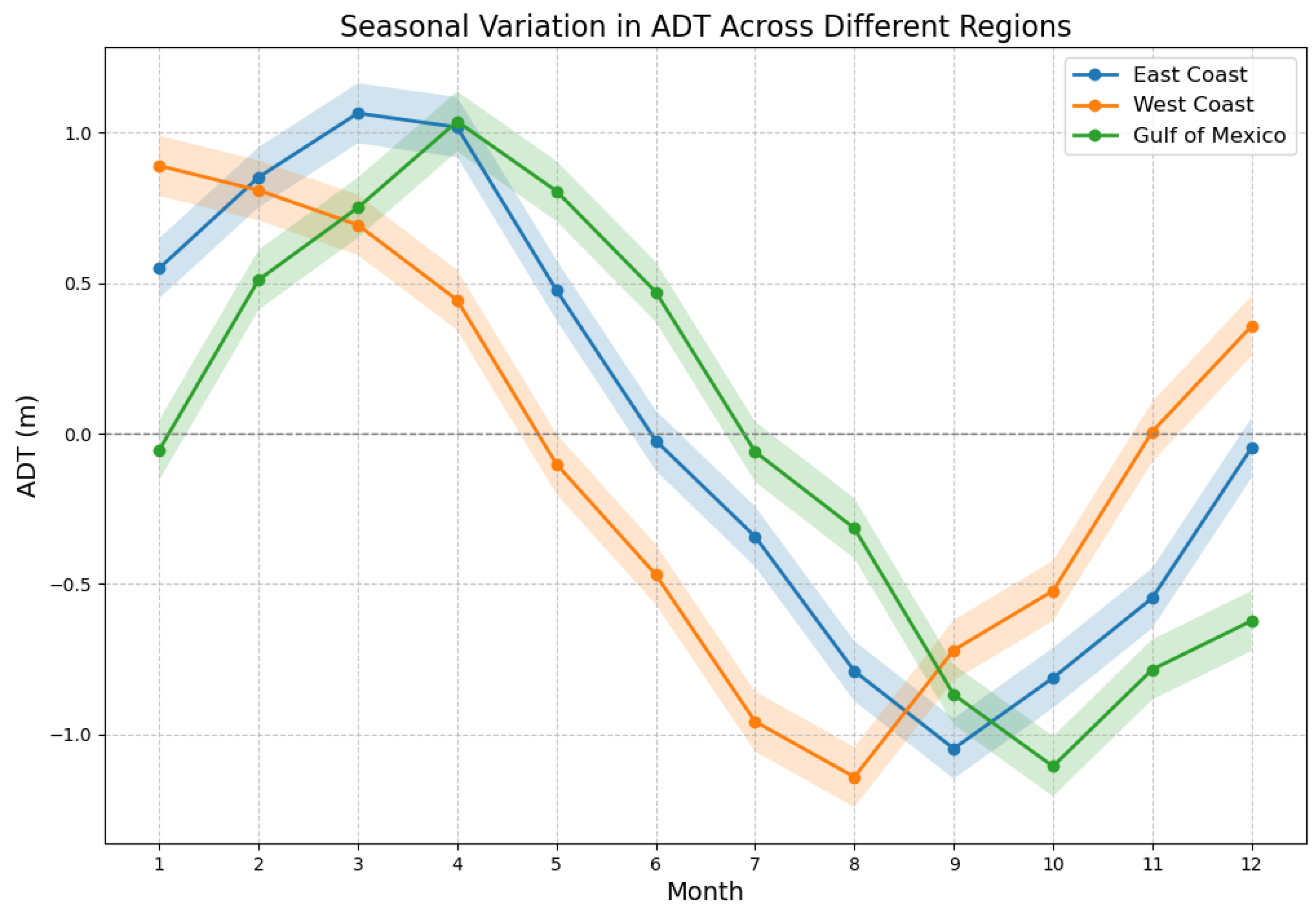
Figure 7.
Regional differences in sea-level rise, highlighting areas with the most significant changes.
Figure 7.
Regional differences in sea-level rise, highlighting areas with the most significant changes.
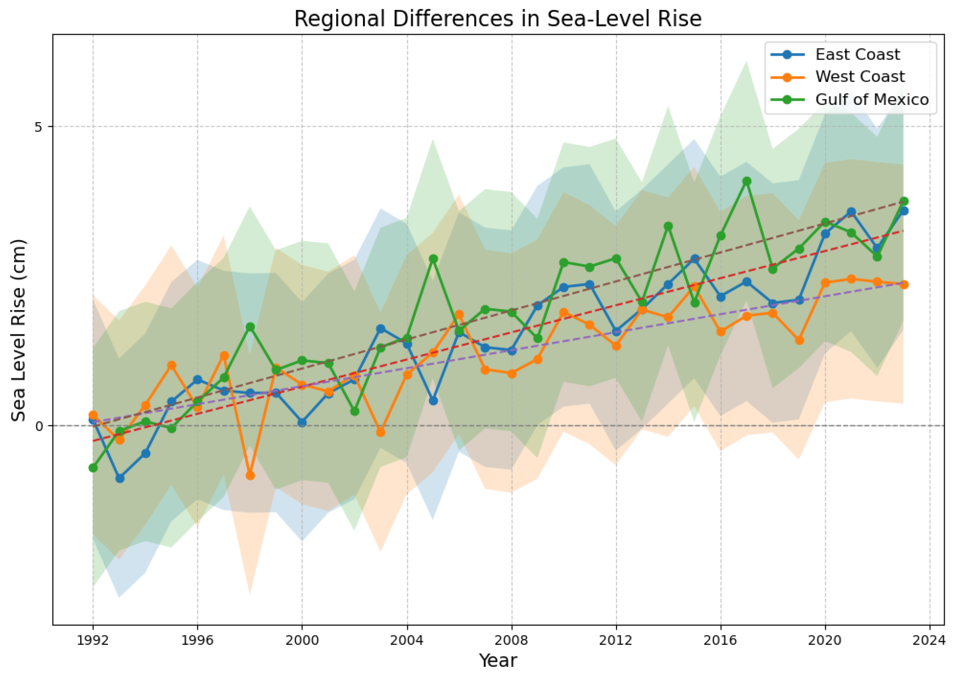
Figure 8.
(a) Comparison of average monthly temperatures between 1995-2000 and 2015-2020. (b) The difference in average monthly temperatures between the two periods.
Figure 8.
(a) Comparison of average monthly temperatures between 1995-2000 and 2015-2020. (b) The difference in average monthly temperatures between the two periods.
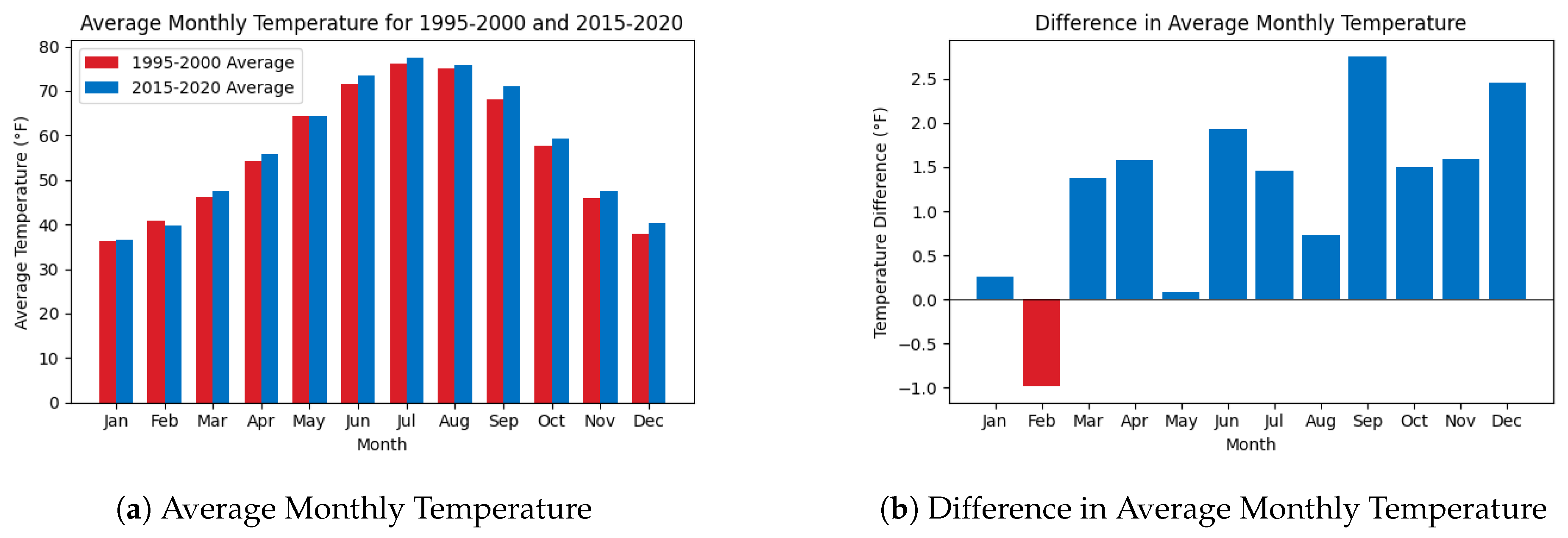
Figure 9.
Seasonal trend in ADT from 2018 to 2023.
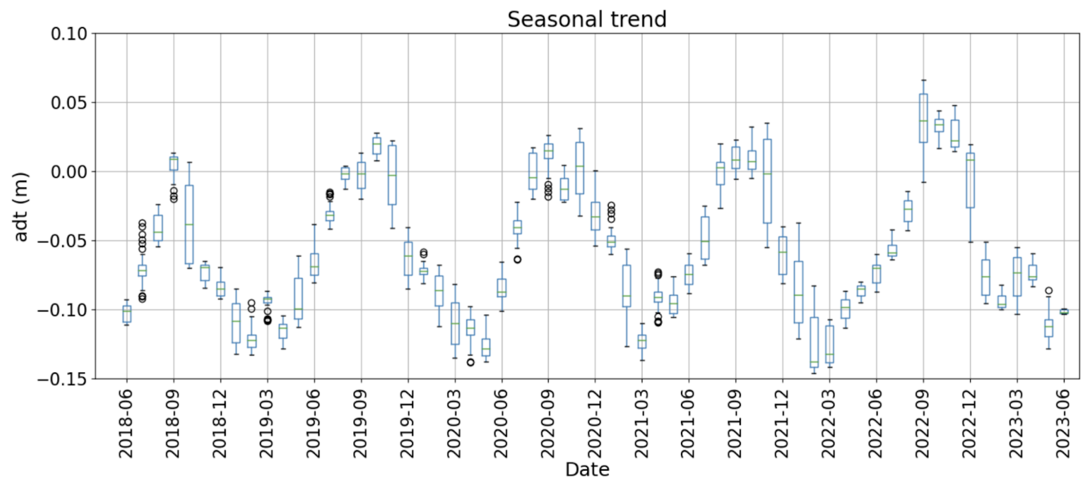
Figure 10.
Raw time-series of ADT for selected latitude-longitude points.
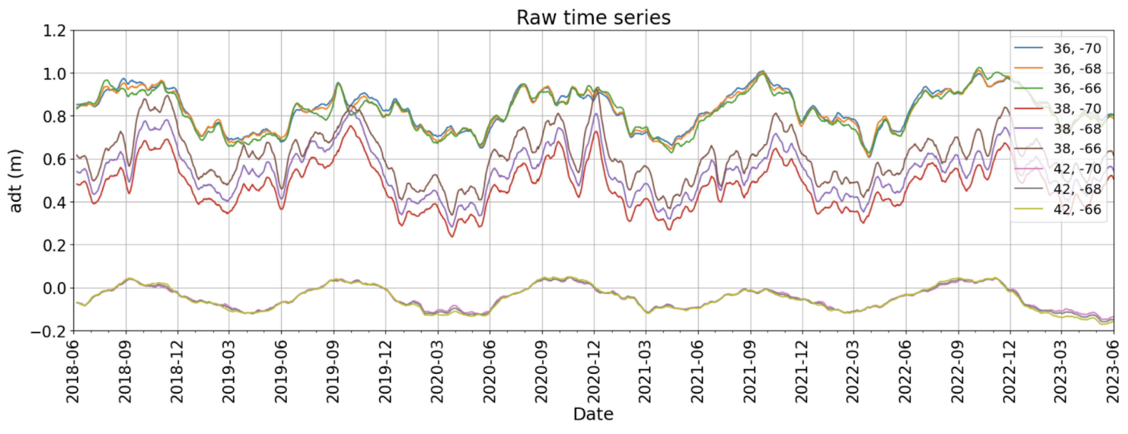
Figure 11.
ADT change between the years 1992 and 2022.
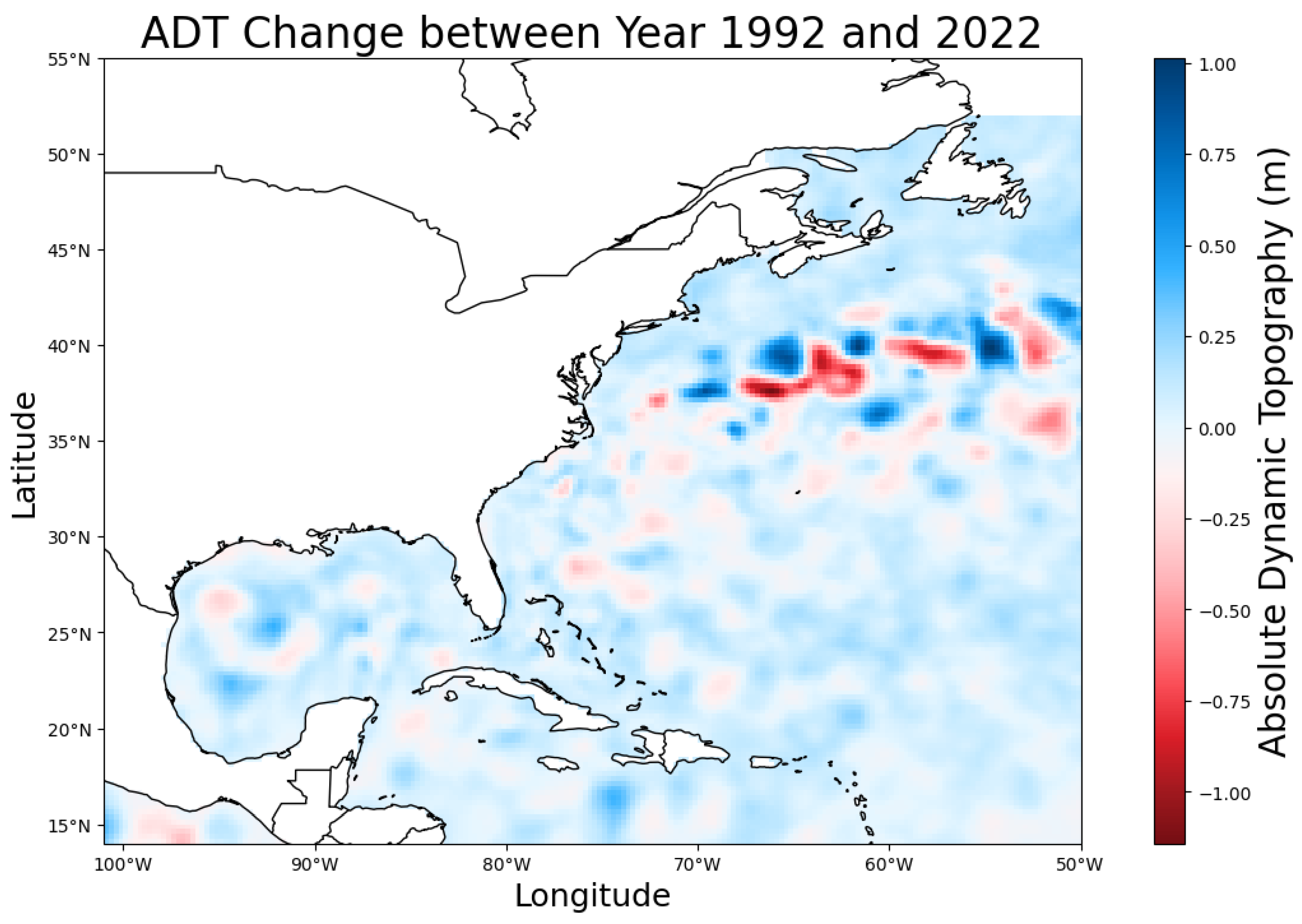
Figure 12.
Average ADT over time from 1992 to 2024.
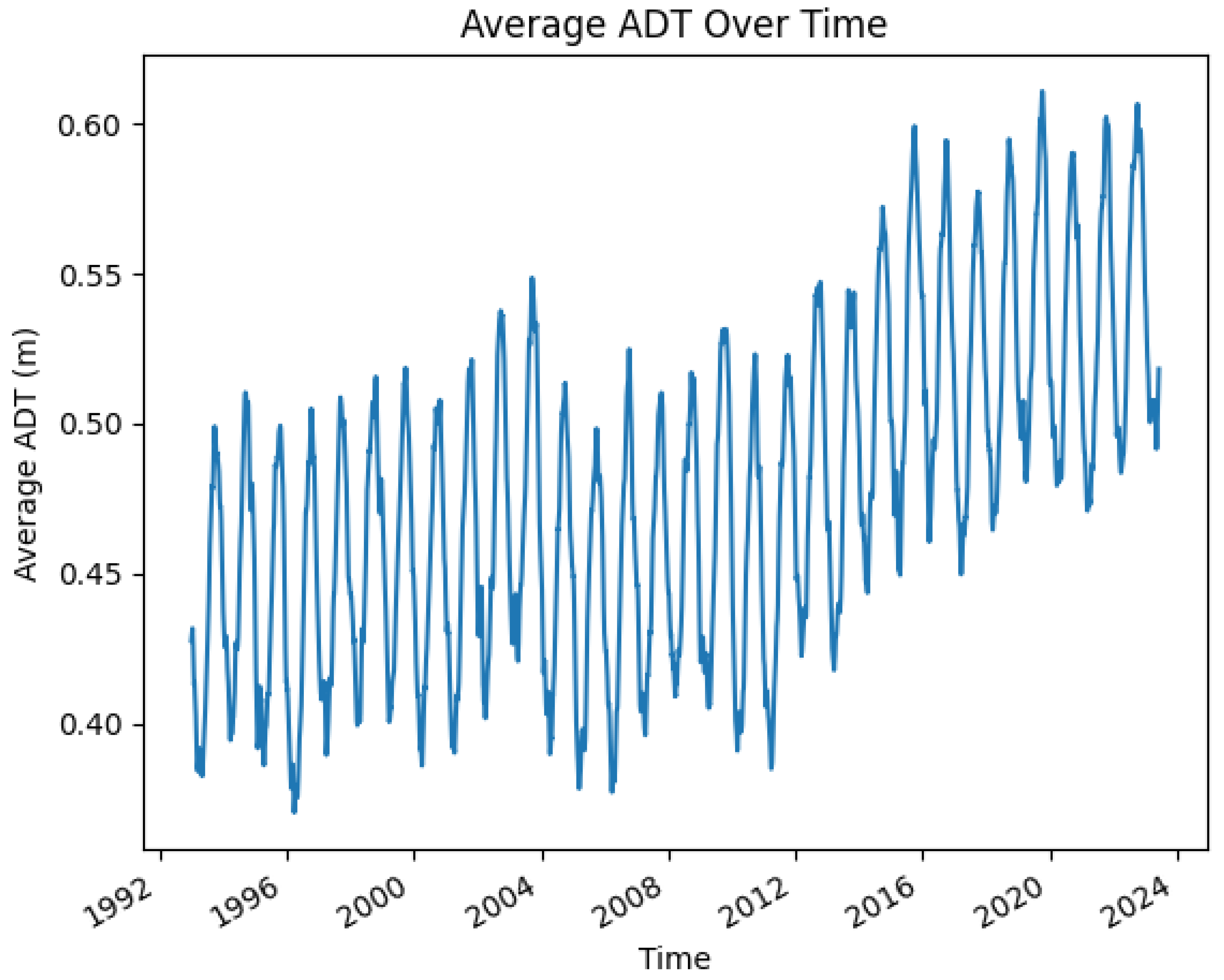
Figure 13.
Global Mean Salinity Anomaly Over Time.
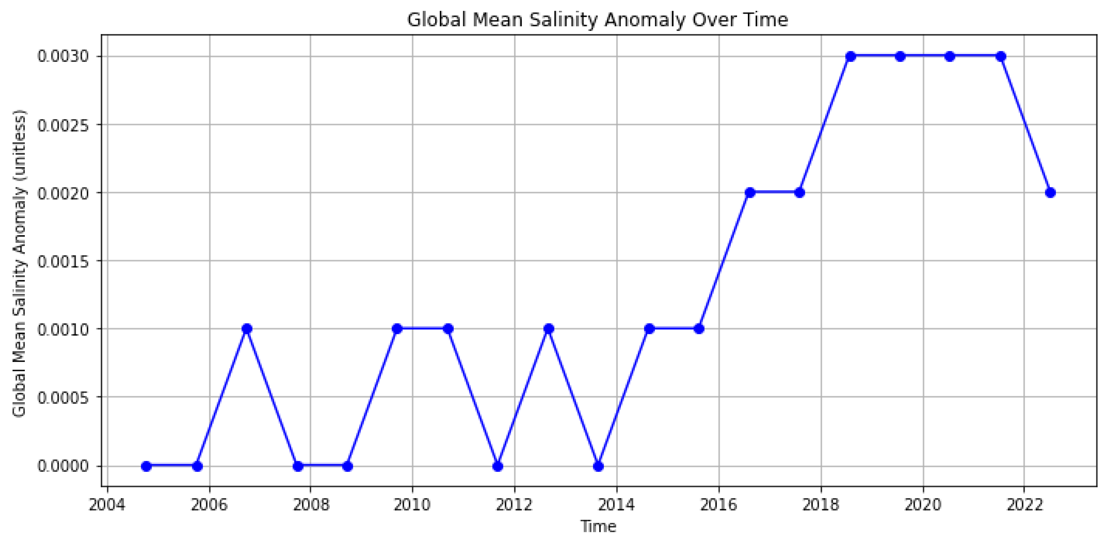
Figure 14.
Ocean Heat Content Over Time.
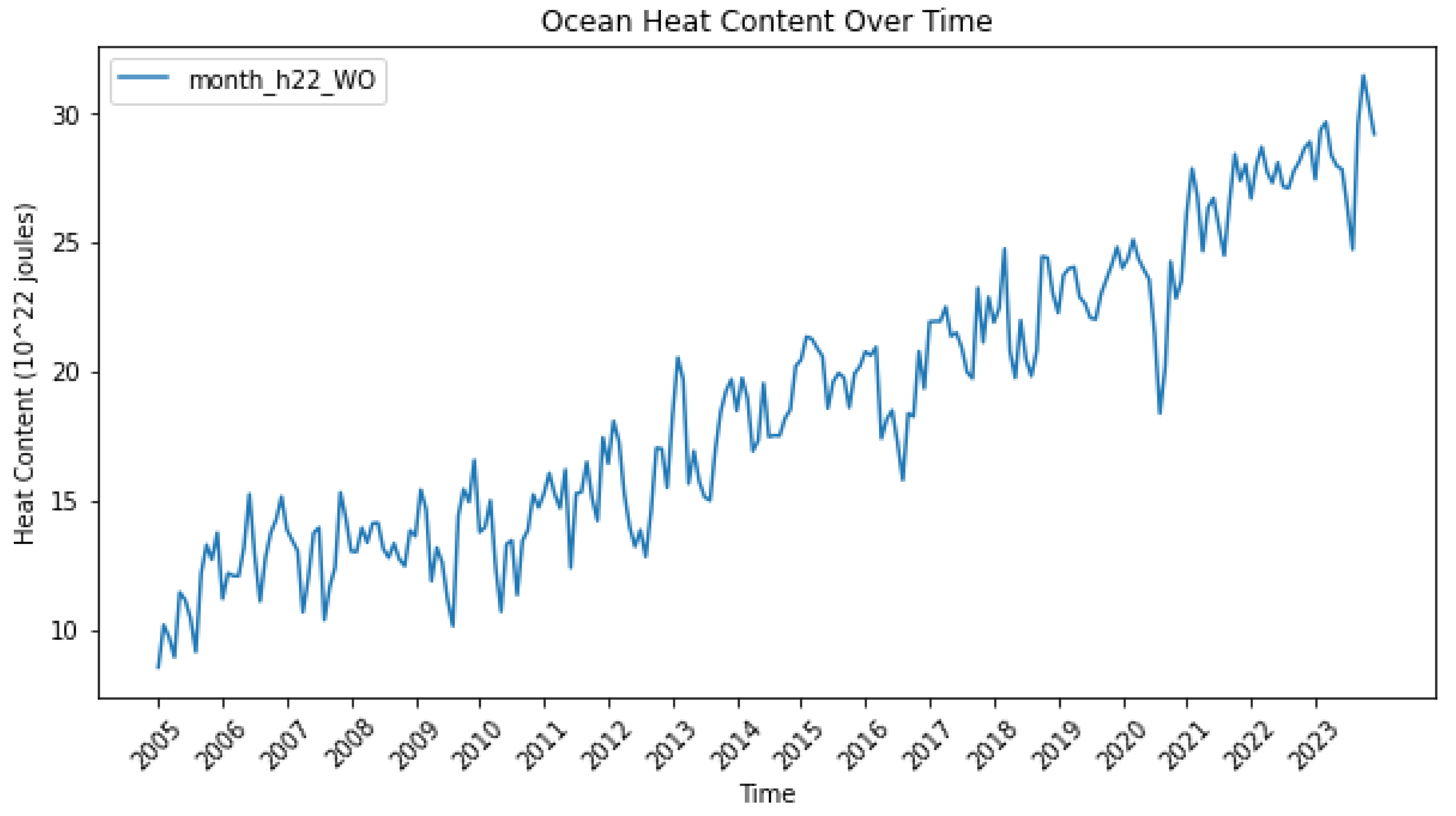
Figure 15.
Statistics metrics of time series for latitude and longitude coordinates. (a) Mean (b) Standard deviation.
Figure 15.
Statistics metrics of time series for latitude and longitude coordinates. (a) Mean (b) Standard deviation.
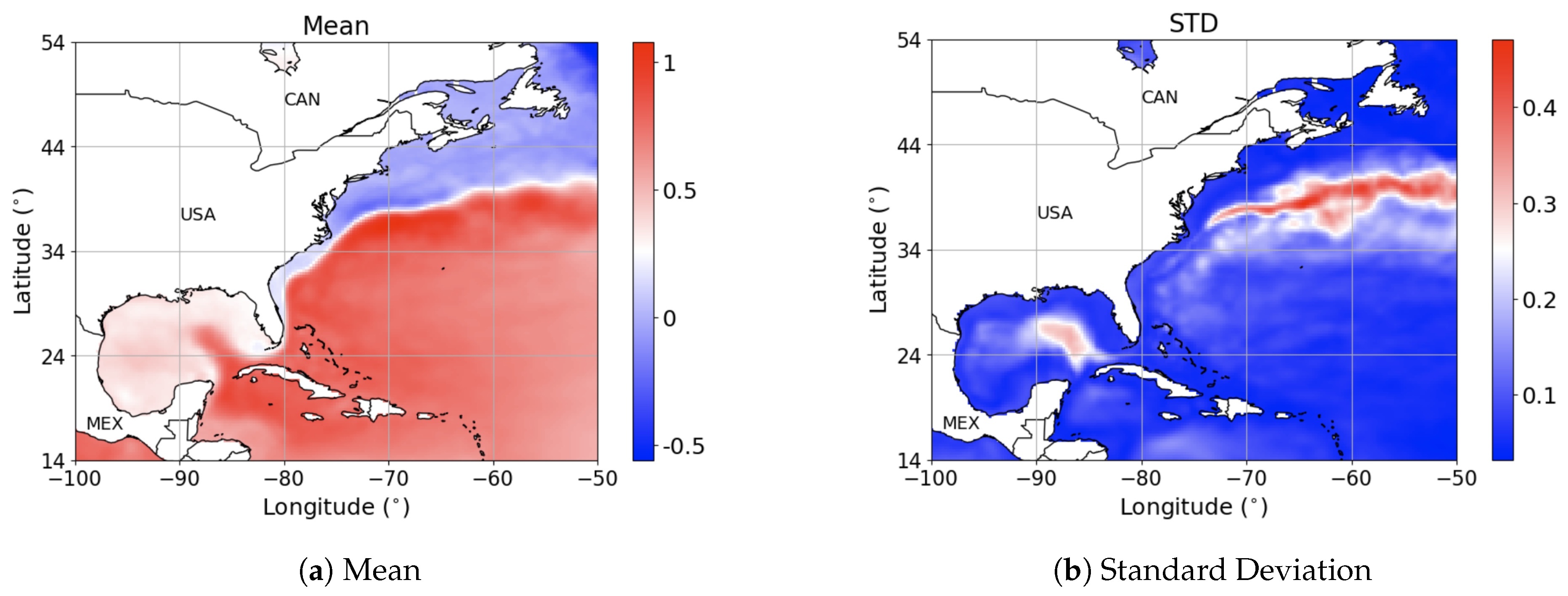
Figure 17.
Distribution of Population and Median Household Income for Coastal Counties.
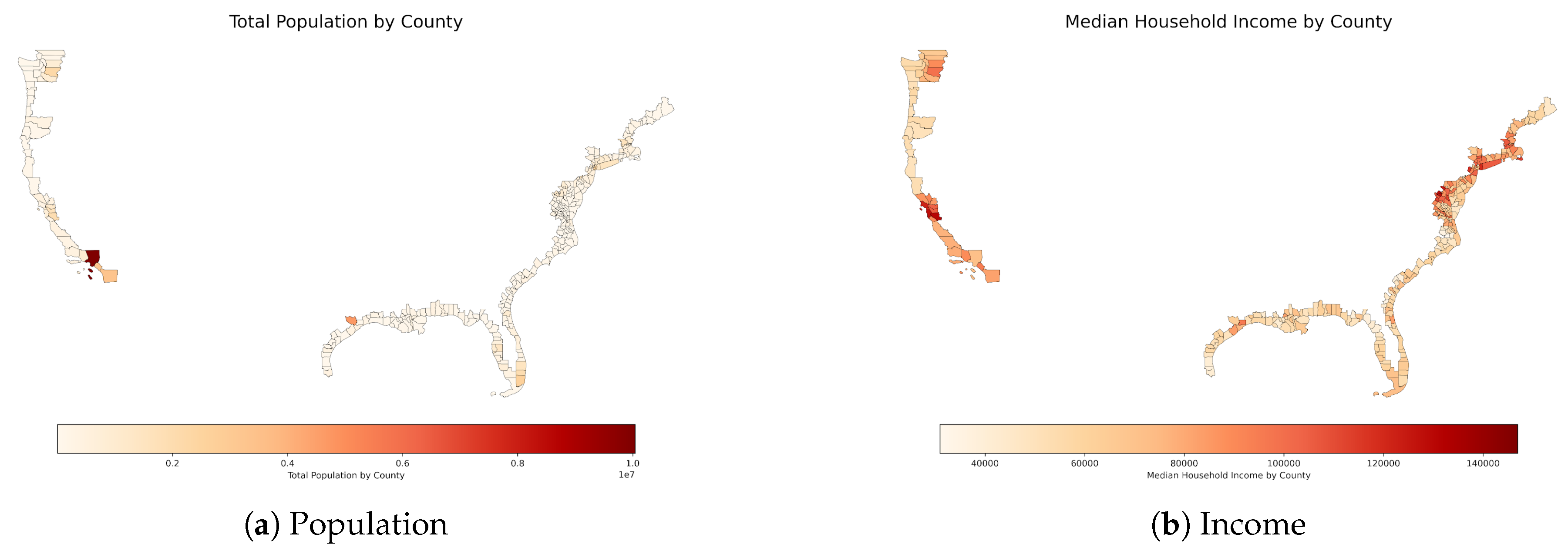
Figure 18.
Low Lying Areas in Coastal U.S. prone to submerging and its outliers. (a) Low-lying areas (b) Outliers.
Figure 18.
Low Lying Areas in Coastal U.S. prone to submerging and its outliers. (a) Low-lying areas (b) Outliers.
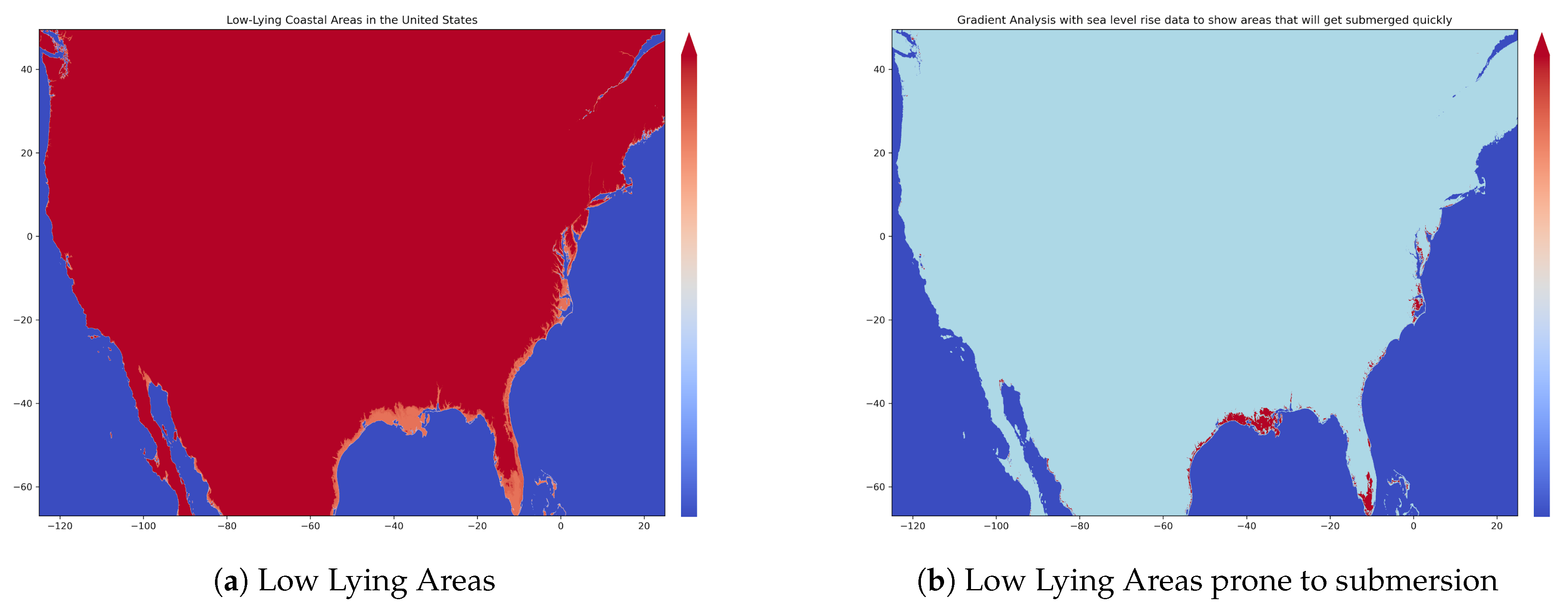
Figure 19.
Marshlands/Wetlands prone to submerging under sea level rise.
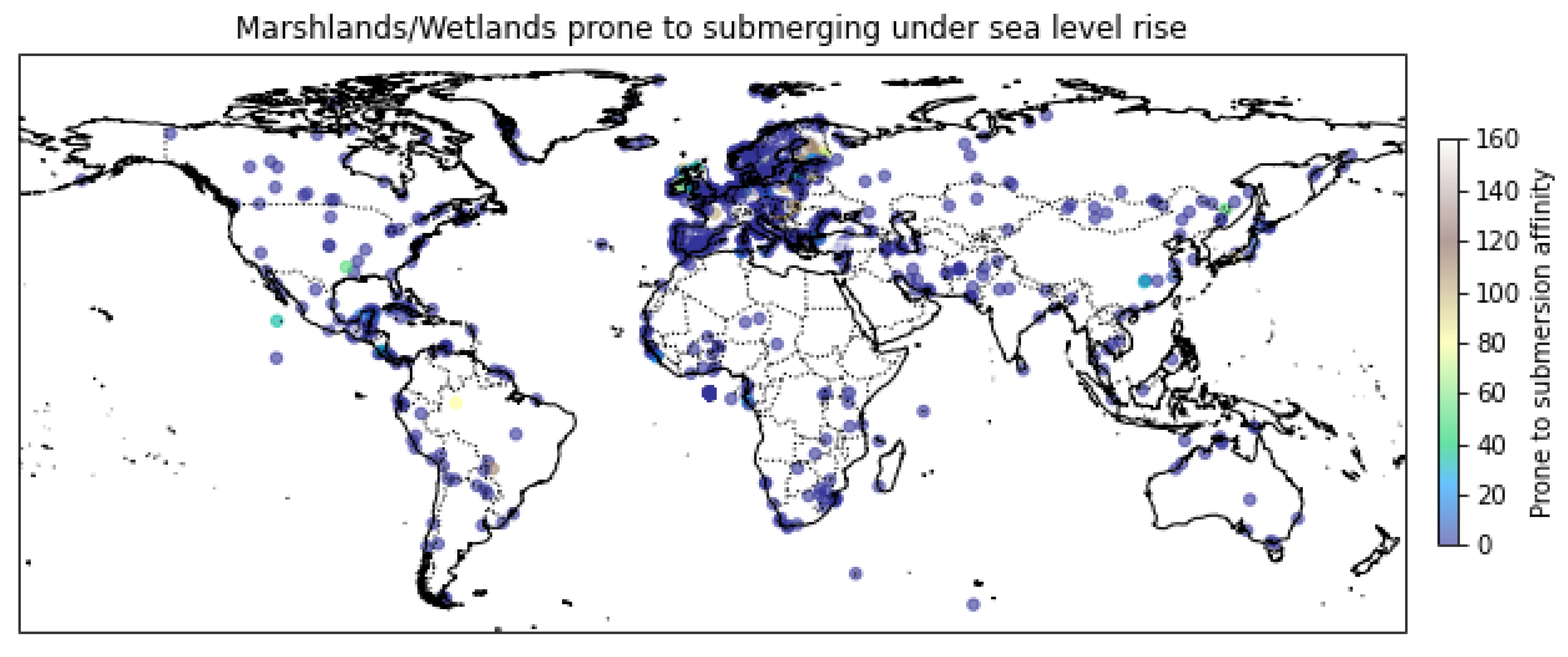
Figure 20.
Employment in All Ocean Sectors by State in 2020.
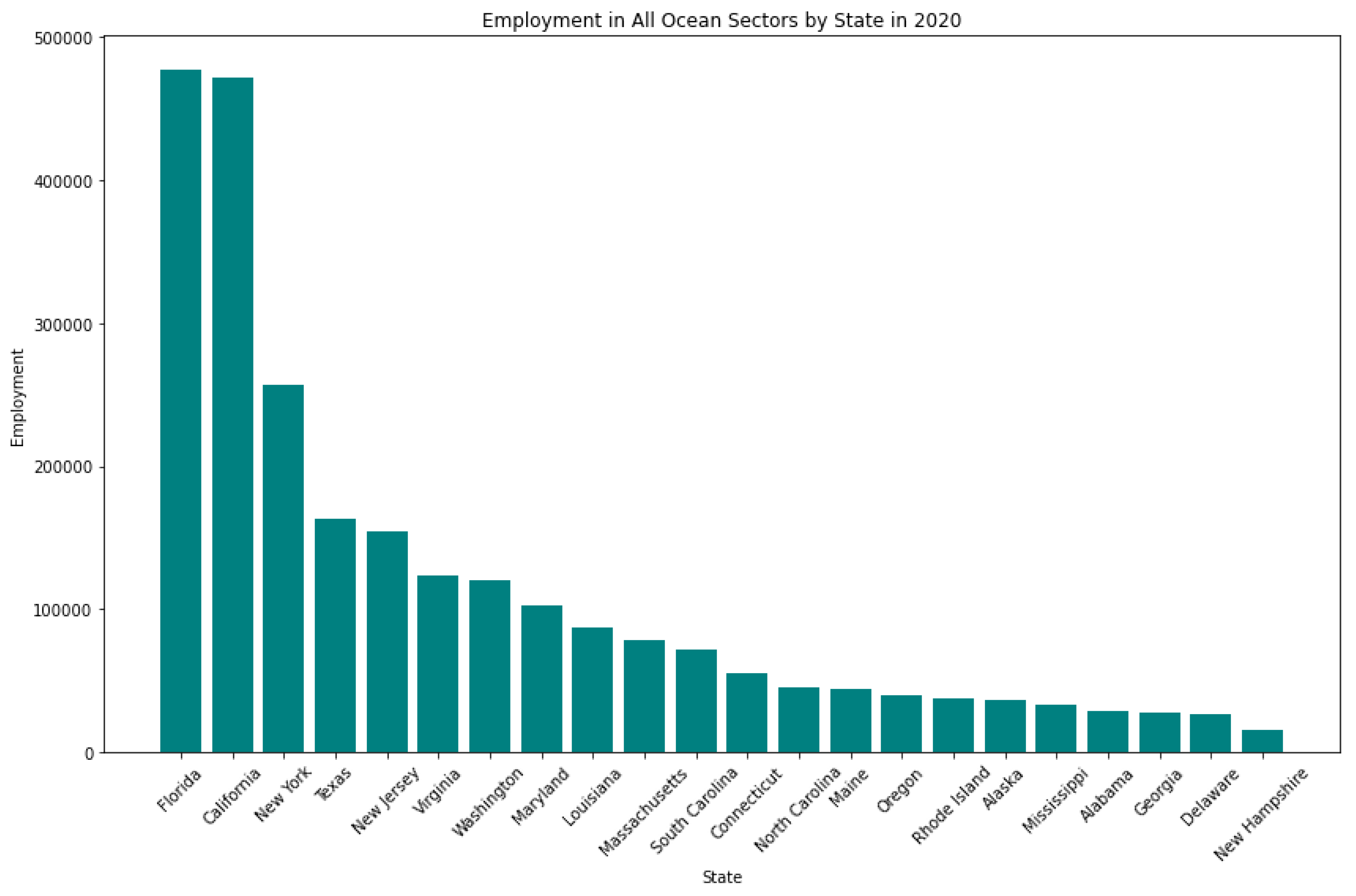
Figure 21.
GDP Trends in All Ocean Sectors for Selected States (2005-2020).
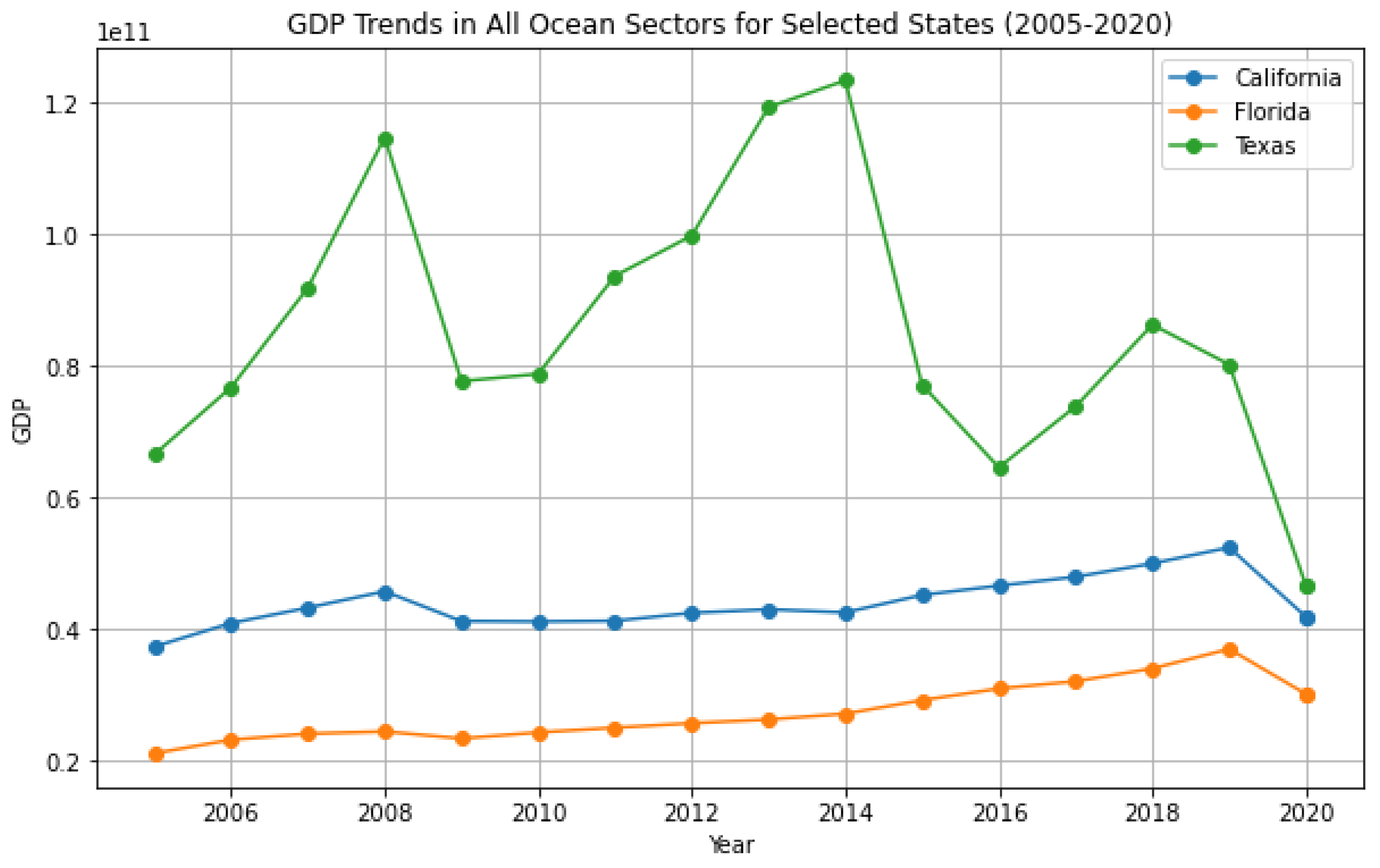
Figure 22.
Employment Trends in All Ocean Sectors (2005-2020).
Disclaimer/Publisher’s Note: The statements, opinions and data contained in all publications are solely those of the individual author(s) and contributor(s) and not of MDPI and/or the editor(s). MDPI and/or the editor(s) disclaim responsibility for any injury to people or property resulting from any ideas, methods, instructions or products referred to in the content. |
© 2024 by the authors. Licensee MDPI, Basel, Switzerland. This article is an open access article distributed under the terms and conditions of the Creative Commons Attribution (CC BY) license (http://creativecommons.org/licenses/by/4.0/).
Copyright: This open access article is published under a Creative Commons CC BY 4.0 license, which permit the free download, distribution, and reuse, provided that the author and preprint are cited in any reuse.


