Submitted:
25 January 2023
Posted:
28 January 2023
You are already at the latest version
Abstract
Observations of ocean surface winds from Indian scatterometer SCATSAT-1 have been combined with background wind field from a numerical weather prediction (NWP) model available at National Centre for Medium Range Weather Prediction (NCMRWF) to generate a 6-hourly gridded hybrid wind product. A distinctive feature of the study is to produce a global gridded wind field from SCATSAT-1 scatterometer passes with spatio-temporal data gaps at regular synoptic hours relevant for forcing models and other NWP studies. This is done by making use of concepts from the modern particle filter technique, which does not represent the model probability density function (PDF) following the Gaussian technique. The 6 hourly hybrid wind is generated for the entire year of 2018 and is validated using the wind speed from daily gridded level-4 SCATSAT-1 winds (L4AW), Cross Calibrated Multi-Platform dataset (CCMP) and global buoy data from National Data Buoy Centre (NDBC). The results indicate potential of the technique to produce scatterometer winds at the desired temporal frequency with significantly less noise and along swath biases. The study shows the generated hybrid winds have very high quality with respect to the already existing daily product available from ISRO.
Keywords:
Winds
; SCATSAT-1
; NCMRWF (National Center for Medium Range Weather Forecasting)
; CCMP (Cross Calibrated Mul-ti-Platform) and Particle filter
1. Introduction
Scatterometers are active microwave radars operating in Ku-Band or C- band, dedicated to the measurement of ocean winds. These space-borne instruments have a long legacy due to continued efforts from various international space agencies. Its journey began in 1978 with short-lived success of Seasat scatterometer by the National Aeronautics and Space Administration (NASA). Further, in 1996 Ku-band scatterometer- the NASA Scatterometer (NSCAT) onboard Advanced Earth Observing Satellite (ADEOS-1) was launched. Following the success of NSCAT, NASA also launched the SeaWinds scatterometer onboard Quick Scatterometer (QuikSCAT) in 1999. At the end of the mission in 2009, NASA launched Rapid Scatterometer (RapidSCAT) on the International Space Station (ISS) in 2014. China also initiated scatterometer missions in 2011 with four scatterometers by the China National Space Administration (CNSA): HaiYang (HY)-2A, HY-2B, HY-2C, and HY-2D. Further, in 2018 China-France cooperation led to the successful launch of a rotating fan beam scatterometer onboard Chinese–French Oceanography Satellite (CFOSAT). European Space Agency (ESA) had a prolonged and continued effort toward C-Band scatterometer. European Remote Sensing Satellites, ERS-1 and ERS-2, officially known as Advanced Microwave Instrument (AMI) scatterometers were launched in 1991 and 1995, respectively. ESA further launched three Advanced Scatterometer (ASCAT) instruments onboard Meteorological Operational-A (METOP-A), METOP-B, and METOP-C in 2006, 2012 and 2018, respectively. A detailed description of the international cooperation in the field of scatterometry can be learned from [1] and [2]. India began its scatterometer program on September 8, 2009 with launch of the first scatterometer called Ocean SCATterometer (OSCAT) onboard Oceansat-2. SCATteromete SATellite-1 (SCATSAT-1) is the second scatterometer mission by the Indian Space Research Organization (ISRO). This study deals with the generation of 6 hourly global gridded wind data from SCATSAT-1.
SCATSAT-1 carries a dual-polarized pencil beam scatterometer dedicated to measuring wind over the ocean. ISRO launched this satellite using Polar Satellite Launch Vehicle (PSLV) C-35 on 26th September 2016 from Sriharikota. It is an active microwave scatterometer operating at a frequency of 13.5 GHz (Ku band) dedicated to measuring the backscatter (σ0) from the ocean surface. This σ0 is eventually used to compute wind vectors over the global oceans. SCATSAT-1 has been instrumental in catering to weather forecasting, cyclone prediction, ocean state prediction, climate change, naval operations, ship routing, etc. The SCATSAT-1 monitors 90% of the global ocean with a repeat orbit of 2 days. It has two beams with horizontal and vertical polarizations with a scan speed of 20.5 rotations per minute. The inner and outer beam makes an incidence angle of 48.9 º and 57.6 º on the ground respectively with a ground resolution of 25 x 25 km. [3]
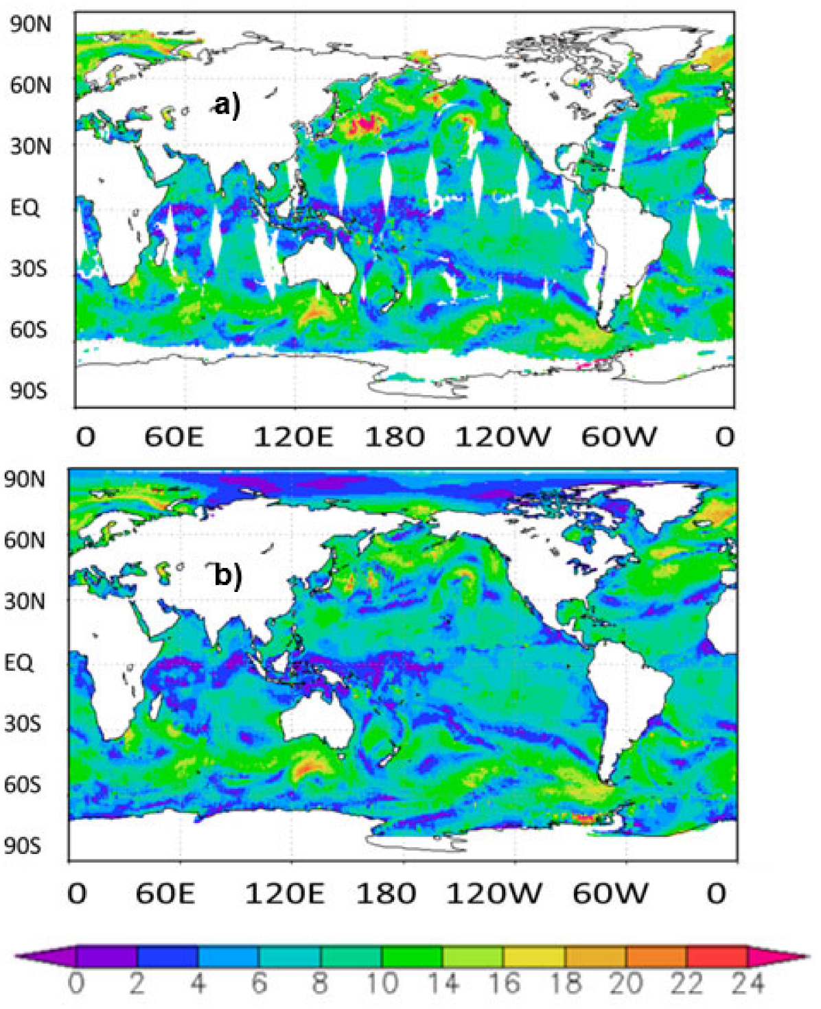
Data processing of the scatterometer involving of converting σ0 into meaningful wind information is extremely complicated with various stages, details of which are available in [4]. While Level-1B (L1B) has actual scan data, Level-2A (L2A) maps σ0 over a geographical area at a fixed grid interval (25 km or 50 km). Level-2B (L2B) combines σ0 and wind information from Numerical Weather Prediction (NWP) models using a geophysical Model Function (GMF) to generate wind vector information corresponding to each cell of the swath. Wind vectors are marked for sea ice and rain flags at this level. Thus, the L2B product provides the wind speed over the global ocean along the passes of the scatterometer as shown in Figure 1. However, user requirement for wind data is stringent. For example, most of the users use wind fields to force their numerical models and thus the wind field has to be gridded preferably at standard synoptic hours of 00, 06, 12, 18 hours. To partially address this requirement the daily analysed wind product from SCATSAT-1 is also made available by ISRO via the official website, www.mosdac.gov.in. This is a value-added product depicting the gridded daily scatterometer analysed wind and is referred to as Level-4 Aanalyzed Wind or L4AW [5]. This is currently the only standard data product form ISRO addressing the requirement of the modelers. In this study, we propose to utilize the particle filter technique for statistically combining SCATSAT-1 and background wind from National Centre for Medium Range Weather Forecasting (NCMRWF) to generate a hybrid wind product every 6 hours (00, 06,12 and 18 UTC). The choice of the particle filter technique is not arbitrary. This widely used option to statistically combine different fields uses optimum interpolation technique. Alternately other ensemble based techniques include the ensemble Kalman filter (EnKF) method of assimilation [6] and particle filter [7]. But unlike other approaches, the particle filter does not consider the apriori assumption of the Gaussianity of the probability distribution function (PDF) of the system. This technique is more suitable where the system is highly non-linear. Recently, particle filter techniques have been successfully utilized in the assimilation of highly non-linear coastal waves in wave models [8]. In similar lines, chlorophyll data have been assimilated in highly nonlinear coupled bio-physical models [9].
2. Data and Methods
In this study, we combine the NCMRWF wind fields with those from L2B product of SCATSAT-1 for 2018. The NCMRWF winds are available from www.ncmrwf.gov.in, which are at a spatial resolution of 25 Km x 25 km and are available at 6 hourly intervals at standard synoptic hours of 00, 06, 12 and 18 UTC. We also utilized the SCATSAT-1 L2B winds and L4AW winds in this study. The L2B wind is used in combination with NCMRWF fields to generate the particle filter-based analyzed wind (PF wind). L4AW is used for validating the PF wind speed. Both these wind products are available at www.mosdac.gov.in, which is the official data dissemination center of ISRO. The L2B data used here are the wind fields along the satellite track and for each day there are approximately 60 track data containing the ascending (south to north) and descending (north to south) passes. These fields are at 25 km spatial resolution. A typical single-day L2B passes of SCATSAT-1 are shown in Figure 1. In this study, we collected the wind fields from Jan 01-00UTC to Dec 3100UTC for the entire 2018. These passes are categorized in synoptic time frames of 00, 06, 12 and 18 UTC by drawing passes within ± 3hours for particular hours. Thus, at end of this exercise observed SCATSAT-1 winds are also available at fixed synoptic hours similar to the NCMRWF background winds.
We compared the resultant hybrid product or PF wind with the existing ISRO-L4AW. This is a gridded daily wind field available at the same spatial resolution [5]. Cross Calibrated Multi-Platform (CCMP) gridded surface vector winds that are generated using satellite, moored buoy, and model wind data are used for validation of the newly generated wind product. These data are available from Remote Sensing Systems (RSS) website, www.remss.com. It combines QuikSCAT and ASCAT scatterometer wind vectors, moored buoy wind data, and ERA-Interim model wind fields using a Variational Analysis Method (VAM) to produce four maps per day as 0.25 x 0.25-degree gridded vector winds. This is an excellent resource for ocean studies and is known for its high accuracy [10,11]. In this study, the Version-2 of CCMP wind is used for 2018. The biases between the CCMP and ISRO daily analysed L4AW wind and particle filter-based winds are calculated for various months to validate the quality of the newly derived wind product for 2018. Apart from this, the NDBC buoy data for 2018 have also been used for validation.
Figure-1.
(a) L2B and (b) L4AW winds from SCATSAT-1 on Dec 1, 2018.
- Particle filter and its implementation procedure
As mentioned, the combination of the SCATSAT –L2B and NCMRWF wind fields is based on the concept of particle filter which is an ensemble-based technique [7]. The novelty of the scheme is that, unlike other ensemble techniques, the particle filter does not impose any restriction on the form of the PDF of the background field. Especially, it does not assume the PDF to be Gaussian, which is the standard assumption of EnKF, and which often gets violated in practice [7,12]. The realistic implementation of the particle filter is clearly explained in [8,9,13].
Particle filter, like any other ensemble based data assimilation scheme, assumes the NCMRWF model wind field background to be stochastic where the state ψ is described by a multivariate PDF, pm(ψ). The observation vector d (which is SCATSAT-1 wind field here) has associated PDF, pd(d). The cornerstone of particle filter is Bayes’s theorem which reads as
The subscripts in the PDFs are dropped assuming that the arguments will clarify which particular PDF is being used. The PDF in the denominator can be easily calculated from the numerator by integration,
Calculation of posterior PDF needs only the knowledge of PDF of observations given the apriori PDF from the background wind fields. The difficulty lies in the calculation of the apriori PDF since the dimension of the state space is prohibitively large. Ensemble-based technique is the solution to this issue. In particle filtering, the background wind PDF is represented by several random draws from the state space, called ensemble members or particles. If there are N such particles, namely with the index i spanning the range 1 to N, the PDF, becomes
Substituting PDF from (3) into the basic equation (1) we obtain
with the weights being given by
Here, the numerator is the PDF of observations given the model state and is known as likelihood. Computation of the likelihood is a must for weight generation. Weights are already normalized so that their sum is unity. Often this likelihood is considered Gaussian, however, there is no compelling reason to do so. Another important aspect is that the likelihoods or the weights, which are just normalized likelihoods are inversely proportional to the distance between a given observation and its model background. Thus, more weight should be given to a particle nearer to a particular observation than to a particle that is farther apart.
We summarised the practical implementation of the method in the flow diagram of Figure 2. The particle generation in this study as shown in the green box of the flow chart is done by adding biases to the background field. It is like perturbing the background field by introducing some random noise. In the initial phase of the study, we added fixed biases with no spatial variation to the entire field to produce a large number of particles (128). RMSE is then obtained by comparing every particle with the SCATSAT-1 observations. There are two major outcomes of this sensitivity experiment. First, applying a particle filter on these particles yielded wind fields that were more skewed to the background field. Second, variation of the RMSE with the introduced bias being governed by the bounds between which we introduced the biases. Thus, the distribution of the bias between its minimum and maximum range is more important than considering a large number of particles. Hence, we varied these additive biases spatially and based them on the monthly biases between the background and the observation fields. As the background field absorbs these biases we generated particles similar to SCATSAT-1 wind field by using the mean difference between observation and background as a perturbation.
Further, these global difference between observation and background are taken on a monthly scale because on a daily scale, global coverage of SCATSAT -1 is not available due to its 2 day repetivity. Bias at a scale of a few days can be influenced by high wind over several locations across the globe facing tropical/subtropical storms. Also, as the winds have great seasonal variability taking bias at more than a month scale would not be suitable for the study. Thus, monthly bias between observation and background was preferred over other alternatives. In addition, following the second conclusion of the sensitivity experiment, when this monthly bias was used as perturbation to the background field, we restricted the total number of the particles to 20 such that with an iterative increment of 5% of the bias field,100% of the bias could be accommodated.
Thus, we selected 20 particles by adding biases to the background field. For each particle between N=1 and N=20 the bias added to background field is NX5 % of the total monthly bias at that grid point. Using initial particles, N=20, and the original observation from SCATSAT-1 L2B, we calculated the weights from (5) to their corresponding particles. The scheme described is popularly referred to as importance sampling, which results in filter degeneracy [7,8], where one particle practically has all the weights.
A remedy to this situation is the idea of resampling. The basic idea behind this resampling is to discard particles with low weights and to retain multiple copies of particles with relatively higher weights so that the total number of particles remains the same. Thus, it is required to calculate the weights and resample the particles and again assign them equal weights (1/N). This weight calculation and resampling is the process by which observations get assimilated into the model. This resampling process is called sequential importance resampling (SIR) [8]. [7] outlined the decision of exactly how many copies of a particle with a relatively high weight has to be retained. In this process, we put N weights after each other on a line [0,1]. A random number is drawn from a uniform density on [0,1/N ]. N-1 line pieces starting from this number with interval length 1/N are laid on the line [0,1]. A particle is chosen when one of the endpoints of these line pieces falls in the weight bin of that particle. The individual particles or ensemble members are not modified during the process to maintain the dynamical balance of the field.
In this case, observations are winds from SCATSAT-1 at each synoptic hour and we generated the particles (N=20) from NCMRWF wind fields by adding spatially varying biases to them. We then collocated these points at the nearest grid point every six hours. Thus, after every six hour interval, distances di between observation and ith particle is computed which are converted to weights following [8]. The raw weights are inverse of these distances (1/di). The constant of proportionality has no role to play as the weights are normalized following equation 5. The particle filter discussed above is then applied and the population of 20 ensembles is resampled keeping the number of ensembles intact. At each synoptic hour, the mean of this resampled population is eventually the newly derived PF wind field. The methodology is summarised in the flow diagram in Figure 2. Figure 3 shows the scatter of the distance of each particle with the biases added for its generation and Figure 4 shows the corresponding weights assigned to it. It can be seen in Figure 3 that as random errors between ±1m/s are introduced in the background wind field, the error between the background and SCATSAT-1 observations starts reducing until 0.4 m/s. After that, the errors again rise. Thus, between 0 and 0.4m/s random error introduced in the background, we get a maxima in the weights (Figure 4). Here, the total number of particles used is 128 and the distribution of the RMSE with introduced bias is typically between the minima and the maxima of the introduced bias. Based on these weights and after the implementation of the sequential importance resampling, some particles with certain introduced random biases are completely removed from the resampled population. These removed particles are those with very low weights. Similarly, some particles with higher weights are repeated with total population remaining the same. Figure 5a shows the variability of biases in the initial and final populations. Thus, for the initial population of the generated particles, the mean perturbation of all 20 particles would be by default 52.5% of monthly bias. However, after the application of the filter procedure the set of particles changes but the total number of particles are same as 20. So, the mean perturbation of the final set of the population would vary largely. For example on 31 May 2018, it was 76.25% of monthly bias. Figure 5b represent the spatial structure of the mean of the bias present in the initial population and resampled population on 31st May 2018.
3. Results and Discussions
We generated the newly derived hybrid wind, which is called PF wind hereafter in the manuscript, for the entire 2018. We did this by combining the L2B wind field from SCATSAT-1 and the background field of NCMRWF and by perturbing to produce 20 particles using spatially varying additive biases. This wind is now at every 6-hour interval like any standard model output. Figure 6 represents the mean wind fields from SCATSAT-1 L2B, the NCMRWF original field and the PF wind speed. Large-scale features in SCATSAT-1 L2B winds are reproduced in the PF wind. Visually the mean field of PF winds is closer to the SCATSAT-1 winds as compared to the winds from the NCMRWF. Lower and higher wind regions are nicely reproduced in the PF winds and are qualitatively closer to the SCATSAT-1
Figure 7 represents the biases between a) NCMRWF wind speed and SCATSAT-1 wind speed b) PF wind speed and SCATSAT-1 wind speed for a 6-monthly duration during Jan-Jun, 2018 and Jul-Dec 2018, respectively. The difference between NCMRWF and SCATSAT-1 wind (7a) has a strong signature of precipitation and cross-scan biases in the satellite data. L2B winds of SCTSAT-1 contain flags for rain, winds and good quality data. We flagged the data for good quality wind data but not for rain. The intention of not using the rain-flag data is to preserve the original observations of SCATSAT-1 and establish the success of the technique in reproducing the scatterometer-like wind field. More difference between the background and observation helps in better testing of the technique. However, the cross-scan bias is a feature that remains an unsolved issue in the L2B data. The biases between SCATSAT-1 and PF wind speed (7b) are much less as compared those between NCMRWF and SCATSAT-1 winds. Globally, the biases near the equator are a little more (negative) as compared to the poles (positive). This is because the biases in the SCATSAT-1 winds near the equator are generally higher due to rain contaminations as compared to those in the NCMRWF wind fields [14]. These biases have significantly reduced by applying the particle filter technique (Figure 7b). This indicates that the particle filter technique is successful in incorporating the SCATSAT-1 wind features and reduces the bias between the original NCMRWF fields and the SCATSAT-1 observations at 6 hourly temporal scales.
To assess the quality of the particle-filter-based product, we compared CCMP wind field, considered as a reference field with the wind speeds from daily L2B-, L4AW-SCATSAT-1 and PF-based reanalysed products. Biases thus computed and shown in Figure 8 and Figure 9 for January and July, 2018, respectively are relatively large and positive in the tropical equatorial regions, gradually decreasing to negative over the mid-latitudes. Out of the three, PF based reanalysis has the least bias between -0.6m/s to 0.9m/s in all regions signifying the effectiveness of the PF method (Figure 8 and Figure 9). Figure 10 shows the global RMSE and standard deviations of the SCATSAT-1 L4AW daily analysed winds and PF winds with respect to the CCMP winds for the entire year. In doing this analysis the daily CCMP winds are averaged to compare with the daily SCATSAT-1 L4AW product. However, we computed RMSE of PF based winds with 6 hourly CCMP winds. PF winds are of better quality to the CCMP winds which is considered reference wind. All global regions like North Atlantic and Pacific and the Southern Ocean show a significant reduction in RMSE from around 3.2 m/s to 2m/s. Another important aspect of the PF wind is a significant reduction in errors along the swath edges appearing due to cross-scan bias. The errors are less even in the equatorial areas. Figure 10 also shows the standard deviations between the CCMP wind and the PF and L4AW winds for the entire 2018. Less RMSE and standard deviation in the newly generated PFwind confirms the better quality of this product.
To further strengthen the validation component, we used the NDBC global buoy data in 2018. We first pre-processed the data to get 10m wind speed and finally collocated with PF wind and L4AW wind to carry out a detailed comparison.
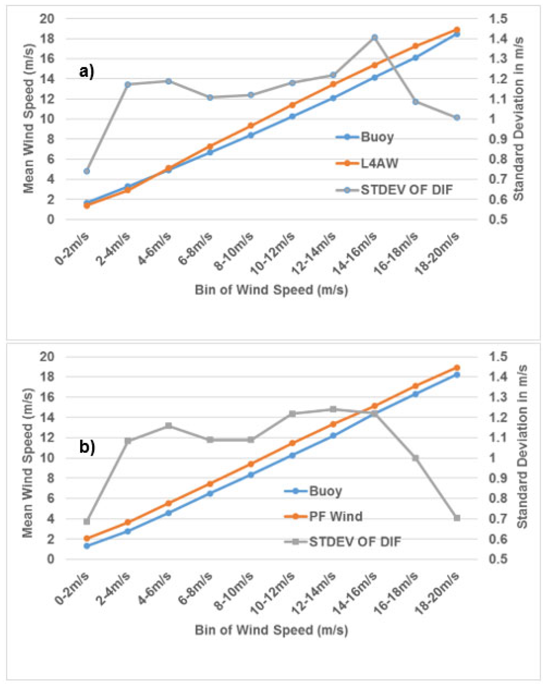
Figure 11 represents the variation of normalized counts at wind speed bins from the buoy, SCATSAT-1 L2B, analyzed daily L4AW and PF winds. The PF wind matches the L2B wind speed more closely compared to L4AW. Figure 12 is the mean wind and standard deviation of the difference between buoy winds and a) analyzed L4AW wind and (b) PF-wind. This binning is calculated on basis of the average of the two wind speeds to avoid statistical effects at the low and high wind. The blue and orange lines represent the mean wind plotted against the primary y-axis (left) while the standard deviation of difference is in the grey line plotted against the secondary y-axis (right). Clearly, the bias between the 6-hourly PF wind and buoy observation is almost constant over every wind speed bin. On the other hand, the bias between L4AW wind and the buoy wind on daily basis varies significantly. The standard deviation of the difference is also low in PF wind for low and high winds. The RMSE and standard deviations for PF wind are 1.82 and 1.12m/s respectively while that of the L4AW are 1.96 and 1.15m/s respectively. The correlation is around 0.81 for PF wind and 0.78 for the L4AW. These results indicate the superiority of the newly suggested approach.
Hence, we generated globally gridded wind product at 6 hourly time interval using PF wind, which is the newly generated hybrid wind produced by combining the NWP model outputs with SCATSAT-1 pass winds This global product generated using particle-filter technique suffices the requirement of modelers/researchers who wish to force their NWP models using these winds. This technique does not assume gaussianity about the system in general. This wind produced for 2018 has been validated using the CCMP winds and NDBC buoy observations. In both validation exercises, the PF wind emerges as a high-quality wind with less noise and reduced bias even along the swath edges compared with the well-established daily SCATSAT-1 wind products known as the analyzed L4AW wind available from ISRO on an operational basis.
4. Summary and Conclusions
The space-based satellite observations of winds are crucial for a variety of oceanographic applications. The main objective of ocean wind measurements using scatterometers is the utilization of winds for ocean state modeling that requires a 6-hourly gridded wind field. Currently, ISRO produces daily gridded scatterometer winds to partially address this issue. In this study, particle filter technique is utilized to generate the gridded 6-hourly wind field at 25 km spatial resolution. This is done by statistically combining the SCATSAT-1 winds and NCMRWF model analysis winds that are also available at 6 hourly intervals at the same resolution. The ways of combining the two different fields are many. The choice of particle filter is an appealing alternative, as it is not bound by restrictions of Gaussian distribution and is most suitable for non-linear systems. In this paper, we have used concepts from this technique for combining the SCATSAT -1 L2B wind fields and NCMRWF wind speed. This wind is generated for 2018 and is validated using the CCMP wind fields and NDBC buoy observations. The bias and RMSE between the CCMP and PF-based wind speed are less. Even the comparison with NDBC buoys, the PF winds are found to be of substantially better quality than L4AW winds. The results unequivocally demonstrate the efficiency and power of this simplified technique based on the particle filter for regeneration of the global gridded scatterometer winds at specific time intervals.
Acknowledgments
This paper contains works done under Technology Demonstration Program (TDP) at Space Applications Centre, ISRO. SAB, MG, AC, NA and RS acknowledge the support given by the Director and Scientist of Management and Information System Area, Space Applications Centre during the TDP. They are also grateful to Dr Nitant Dube, Dr Atul Varma and Dr B. Kartikeyan for their important and critical suggestions during various phases of the project. MMA is thankful to COSPS/FSU, APSDMA and KL University for the support and encouragement.
Conflicts of Interest
The authors have no potential conflict of interest.
References
- Liu, L.W Progress in Scatterometer Application. Journal of Oceanography, 2002, 58, 121-136. [CrossRef]
- Singh, S.; Tiwari, R.K., Sood, S., Kaur, R.; Prashar, S. The Legacy of Scatterometer. IEEE Geoscience And Remote Sensing Magazine, June 2022, 39-65. [CrossRef]
- Bhowmick, S.A.; Cotton, J.; Fore, A.; Kumar, R.; Payan, C; Rodriguez, E.; Sharma, A.; Stiles, B.; Stoffelen A.; Verhoef A. An assessment of the performance of ISRO’s Scatsat-1 Scatterometer. Current Science. 2019,117, 6, 25, 959-972.
- Mankad, D.; Sikhakolli, R.; Kakkar, R.; Saquib, Q. SCATSAT-1 Scatterometer Data Processing Current Science. 2019, Vol. 117, 6, 25,950-958.
- Chakraborty, A.; Varma, AK.; Kumar. R. On the Generation of Daily Gridded Ocean Surface Vector Wind Products from Scatsat-1. IEEE Geoscience and Remote Sensing Letters. 2020. [CrossRef]
- Evensen, G. Data assimilation: the ensemble Kalman filter. Berlin: Springer. 2009.
- Van Leeuwen, P. J. Particle filtering in geophysical systems. Monthly Weather Review. 2009,137, 4089–4114. [CrossRef]
- Bhowmick S A; Ratheesh, S.; Sharma, R.; Basu, S; Kumar, R. A Simplified Assimilation Scheme for a Coastal Wave Model Using Concepts of Particle Filter. Pure and Applied Geophysics. 2020, 177,1167-1181. [CrossRef]
- Ratheesh, S.; Chakraborty, A.; Sharma, R.; Basu, S. Assimilation of satellite chlorophyll measurements into a coupled biophysical model of the Indian Ocean with a guided particle filter. Remote Sensing Letters. 2016, 7(5), 446–455. [CrossRef]
- Atlas, R.; Hoffman, R.N., Ardizzone, J., Leidner, S.; Jusem, J.C.; Smith, D.K.; Gombos, D. A cross-calibrated, multiplatform ocean surface wind velocity product for meteorological and oceanographic applications. Bull. Amer. Meteor. 2019, 92, 157-174. [CrossRef]
- Mears, C. A.; Scott, J.; Wentz, F. J.; Ricciardulli, L.; Leidner, S. M.; Hoffman, R.; Atlas, R. A Near Real Time Version of the Cross Calibrated Multiplatform (CCMP) Ocean Surface Wind Velocity Data Set. Journal of Geophysical Research: Oceans. 2019, 124, 6997– 7010. [CrossRef]
- Van Leeuwen, P. J. Nonlinear data assimilation in geosciences: an extremely efficient particle filter. Quarterly Journal of the Royal Meteorological Society. 2010, 136, 1991–1999. [CrossRef]
- Mattern, J. P.; Dowd, M.; Fennel, K. Particle filter-based data assimilation for a three-dimensional biological ocean model and satellite observations. Journal of Geophysical Research. 2013,118, 2746–2760. [CrossRef]
- Kumar R.; Bhowmick S.A.; Chakraborty A.; Sharma A.; Sharma, S.; Seemanth M.; Gupta M.; Chakraborty P.; Modi J.; Misra T. Post-launch calibration–validation and data quality evaluation of SCATSAT-1. Current Science. 2019, 117, 6, 25,973-982. [CrossRef]
Figure 2.
Particle filter implementation steps.
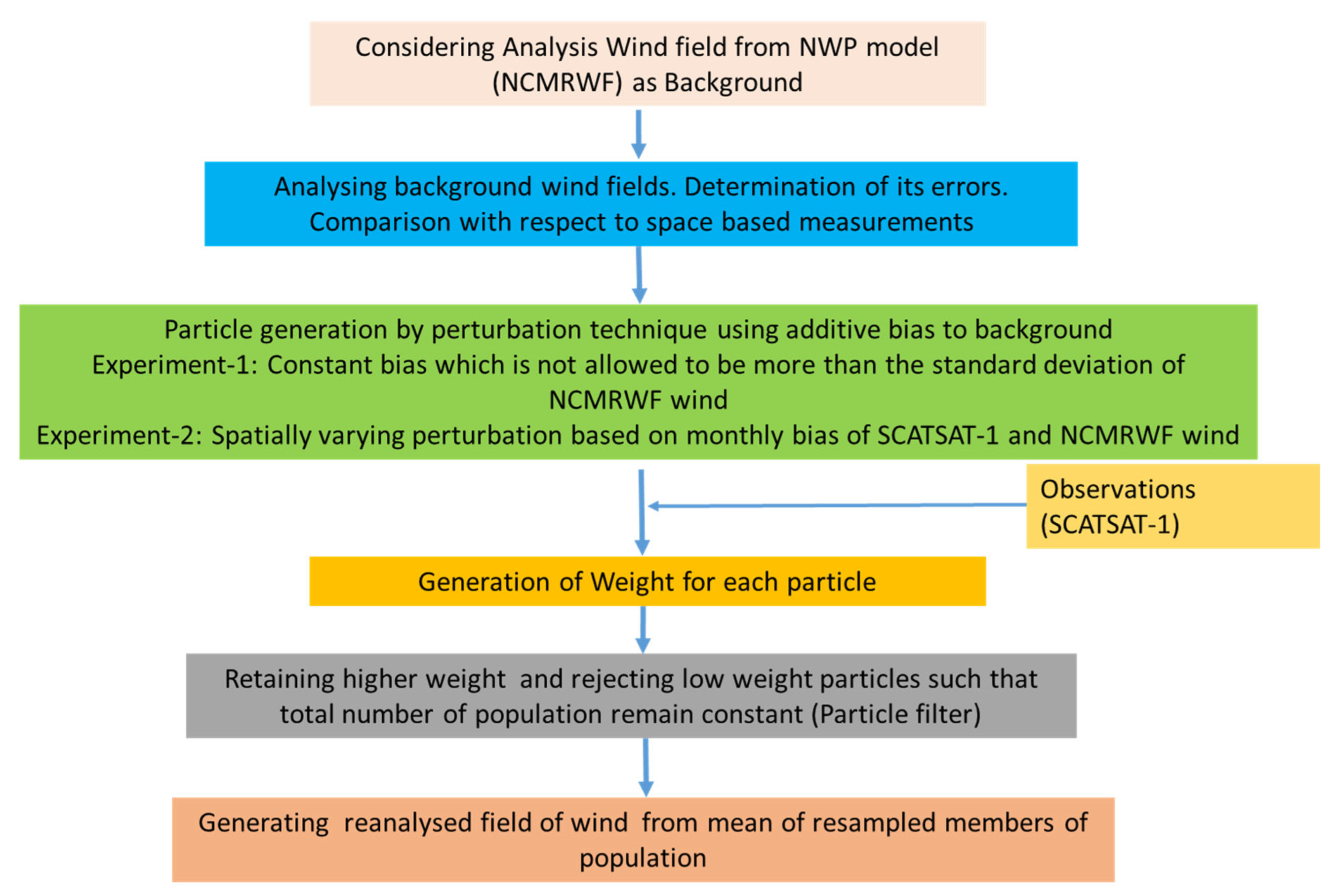
Figure 3.
Variation of RMSE of each ensemble w.r.t introduced biases in wind fields.
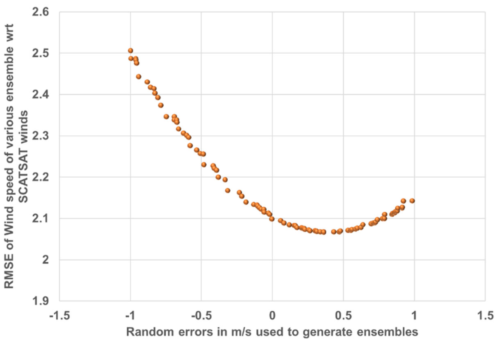
Figure 4.
Variation of weights in each ensemble w.r.t introduced biases in wind fields.
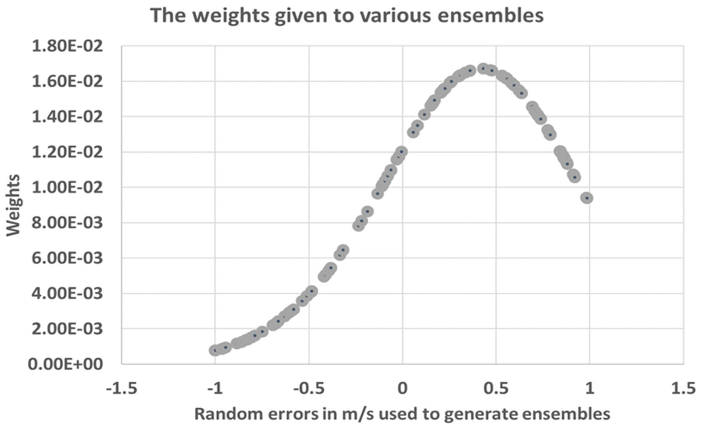
Figure 5.
(a) Histogram of the bias in initial and final population. (b) mean perturbation in initial population (top) and same in resampled population (bottom) on 31 May 2018.
Figure 5.
(a) Histogram of the bias in initial and final population. (b) mean perturbation in initial population (top) and same in resampled population (bottom) on 31 May 2018.
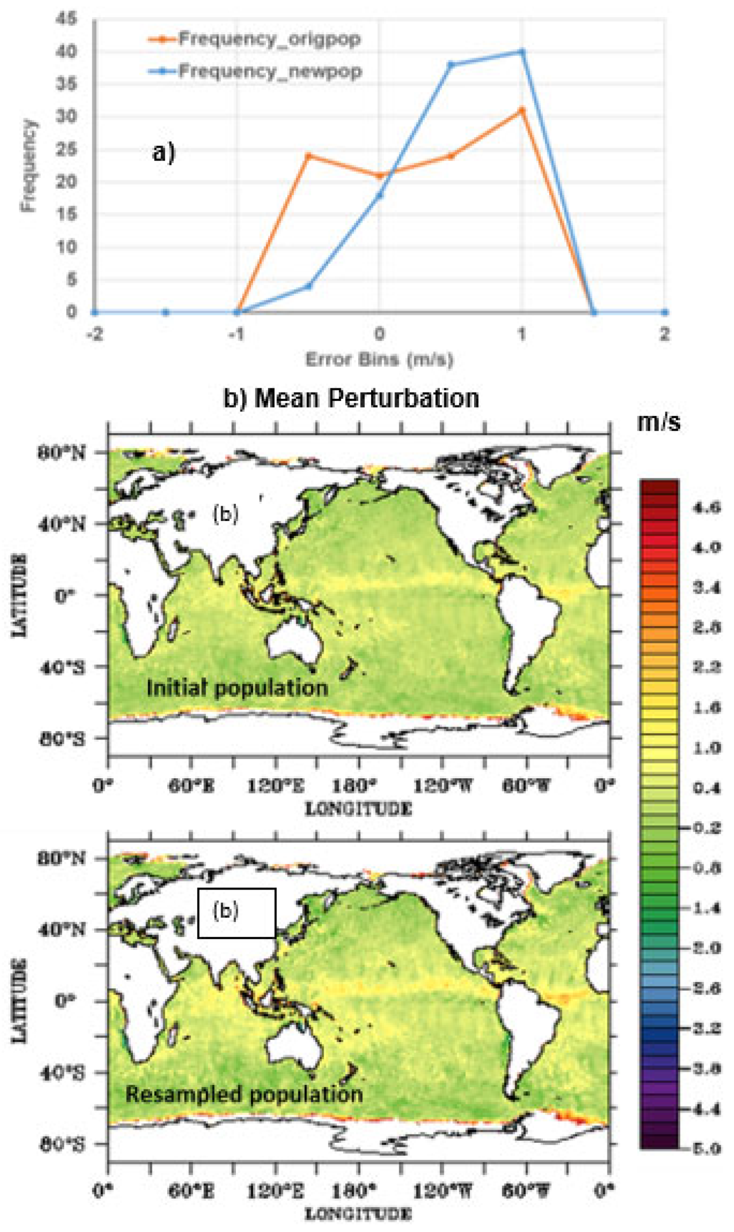
Figure 6.
Mean wind field Jan-Dec 2018 from (a) SCATSAT-1 (b) NCMRWF and (c) Particle filter-based Reanalysis.
Figure 6.
Mean wind field Jan-Dec 2018 from (a) SCATSAT-1 (b) NCMRWF and (c) Particle filter-based Reanalysis.
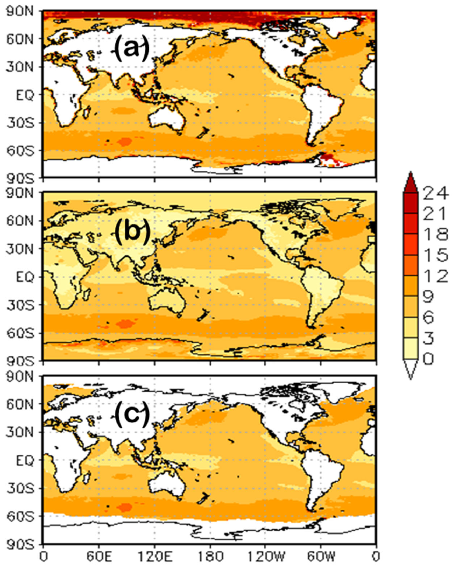
Figure 7.
Bias between (a) NCMRWF wind speed and SCATSAT-1 wind speed (b) Particle filter-based reanalyzed wind speed and SCATSAT-1 wind speed between Jan-Jun 2018 and Jul-Dec 2018 winds as compared to the NCMRWF winds. This indicates the successful statistical inclusion of the SCATSAT-1 measurements in a background field using the particle filter technique.
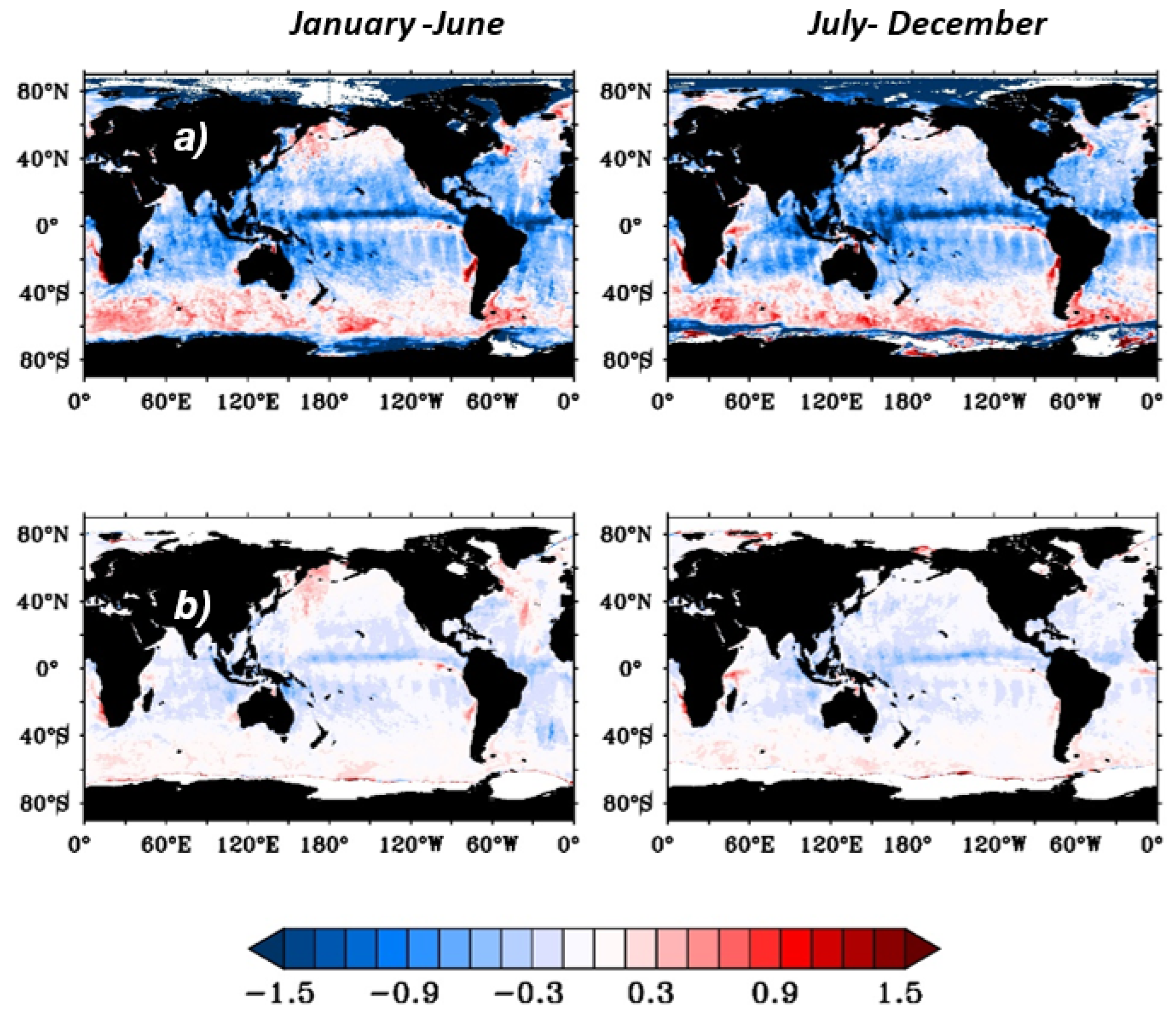
Figure 8.
The spatial distribution of bias in wind speed (m/s) between CCMP wind speed and (i) SCATSAT-1 L2B wind speed (top panel), (ii) Particle filter based reanalysed wind speed (middle panel) (iii) SCATSAT-1 L4AW wind speed (bottom panel) during January 2018.
Figure 8.
The spatial distribution of bias in wind speed (m/s) between CCMP wind speed and (i) SCATSAT-1 L2B wind speed (top panel), (ii) Particle filter based reanalysed wind speed (middle panel) (iii) SCATSAT-1 L4AW wind speed (bottom panel) during January 2018.
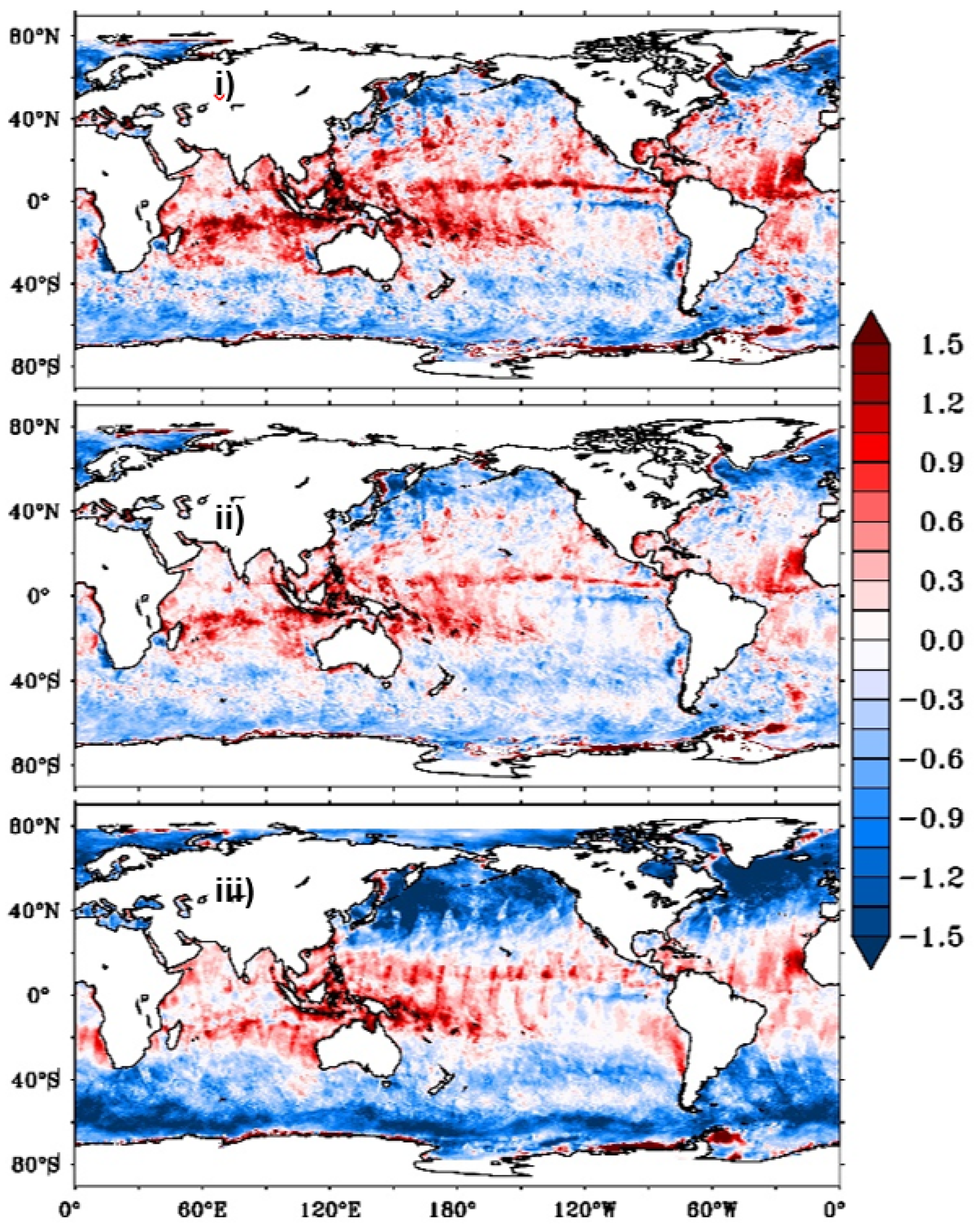
Figure 9.
The spatial distribution of bias in wind speed (m/s) between CCMP wind speeds and (i) SCATSAT-1 L2B wind speed (top panel), (ii) Particle filter based reanalysed wind speed (middle panel) (iii) SCATSAT-1 L4AW wind speed (bottom panel) during July 2018.
Figure 9.
The spatial distribution of bias in wind speed (m/s) between CCMP wind speeds and (i) SCATSAT-1 L2B wind speed (top panel), (ii) Particle filter based reanalysed wind speed (middle panel) (iii) SCATSAT-1 L4AW wind speed (bottom panel) during July 2018.
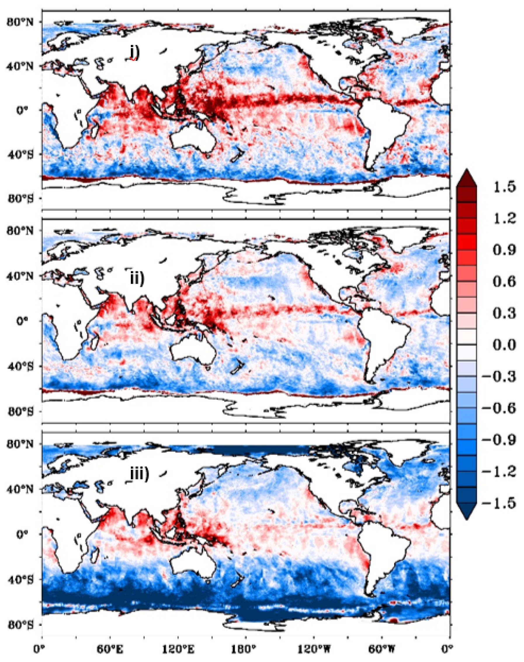
Figure 10.
The spatial distribution of RMSE (top panel) and standard deviation (bottom panel) in wind speed (m/s) between daily CCMP winds and (a) Particle filter based reanalysed wind speed and (b) SCATSAT-1 L4AW wind speed during 2018.
Figure 10.
The spatial distribution of RMSE (top panel) and standard deviation (bottom panel) in wind speed (m/s) between daily CCMP winds and (a) Particle filter based reanalysed wind speed and (b) SCATSAT-1 L4AW wind speed during 2018.
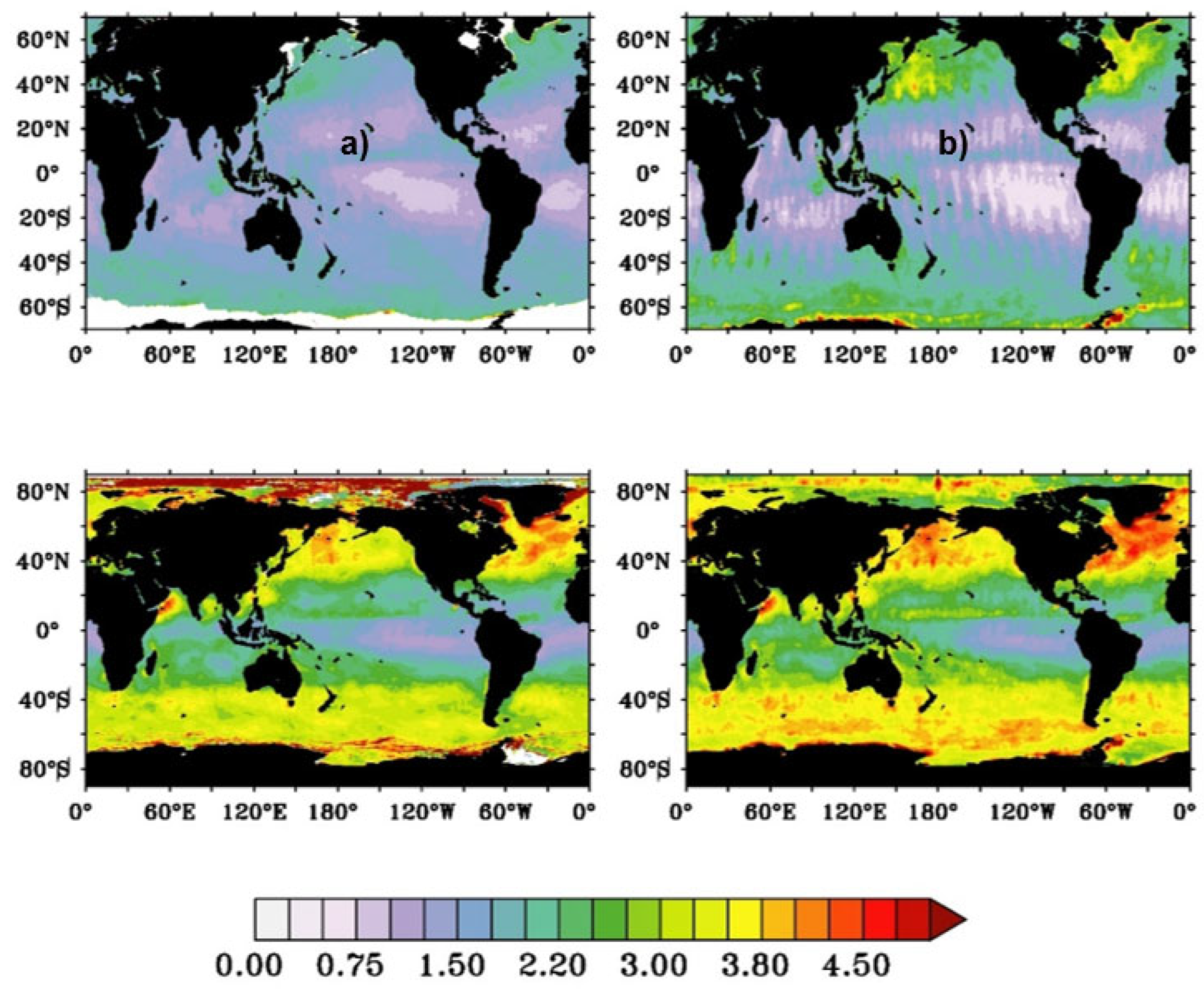
Figure 11.
The normalized histogram of SCATSAT-1 L2B, daily L4AW wind speed, particle filter-based reanalyzed wind speed and wind speed observations from NDBC global buoys.
Figure 11.
The normalized histogram of SCATSAT-1 L2B, daily L4AW wind speed, particle filter-based reanalyzed wind speed and wind speed observations from NDBC global buoys.
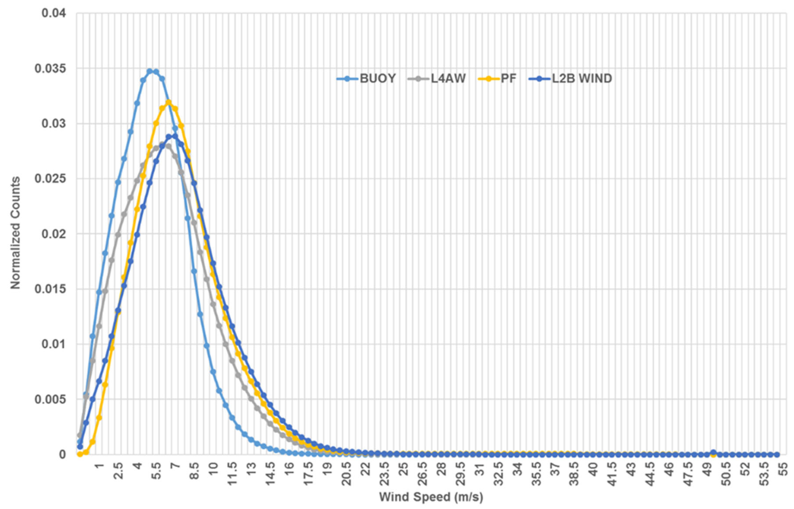
Figure 12.
Mean wind and standard deviation of the difference between NDBC global buoy winds and (a) analyzed L4AW wind and (b) PF-wind for the year 2018.
Figure 12.
Mean wind and standard deviation of the difference between NDBC global buoy winds and (a) analyzed L4AW wind and (b) PF-wind for the year 2018.
© 2023 by the authors. Licensee MDPI, Basel, Switzerland. This article is an open access article distributed under the terms and conditions of the Creative Commons Attribution (CC BY) license (http://creativecommons.org/licenses/by/4.0/).
Copyright: This open access article is published under a Creative Commons CC BY 4.0 license, which permit the free download, distribution, and reuse, provided that the author and preprint are cited in any reuse.


