
Submitted:
25 October 2025
Posted:
27 October 2025
You are already at the latest version
Abstract
This study investigates the impact of high-resolution Sea Surface Temperature (SST) boundary conditions on atmospheric simulations over the southwestern Atlantic Ocean (12–27°S, 32–48°W). Numerical experiments were conducted using the WRF (Weather Research and Forecasting) model with two distinct SST configurations: standard resolution GFS SST data ( 0.5°) and high-resolution RTG-SST-HR satellite-derived data ( 0.083°). Simulations covered contrasting seasonal periods (January and July 2016) to capture varying upwelling intensities and atmospheric circulation patterns. Model performance was evaluated against observational data from the Brazilian National Buoy Program (PNBOIA) using statistical metrics including Root Mean Square Error (RMSE) and Pearson correlation coefficients for wind components, air temperature, and sea-level pressure. The high-resolution SST experiment demonstrated significant improvements in wind field representation, with RMSE reductions of up to 0.5 m/s for zonal wind components and correlation improvements of approximately 0.1 across multiple validation sites. Most notably, the enhanced SST resolution enabled better representation of mesoscale atmospheric systems, including improved organization and intensification of cyclonic systems in the region’s primary cyclogenesis corridor. The RTG-SST data captured sharp thermal gradients and coastal upwelling signatures that were spatially smoothed in the GFS fields, leading to more realistic surface heat flux patterns and atmospheric boundary layer dynamics. These improvements were particularly pronounced during summer months when thermal gradients were strongest, highlighting the critical importance of accurate SST representation for capturing high-intensity atmospheric phenomena in regions of strong air-sea interaction.
Keywords:
Sea Surface Temperature
; surface winds
; ocean-atmosphere interaction
; WRF model
1. Introduction
Sea Surface Temperature SST is a physical variable that plays a key role in the transfer of longwave radiation from the oceans to the atmosphere, as well as in the exchange of latent and sensible heat with the lower layers of the ocean column [1]. SST is widely used in scientific studies due to its potential to describe ocean dynamics and circulation, as well as its importance in ocean-atmosphere interaction. It also serves as an essential indicator for tracking phenomena related to interannual variability, such as the El Niño-Southern Oscillation (ENSO), and seasonal variations.
Infrared sensors onboard satellites measure radiation from a thin skin layer at the ocean surface [2], a phenomenon confirmed by several authors [3,4]. This skin layer may differ by a few tenths of a degree from temperatures measured just centimeters below the surface. While the thickness of this layer is typically less than one millimeter [4], its actual depth depends on local energy flux across the ocean surface and molecular transport under calm sea conditions.
The skin layer can be disrupted by intense meteorological conditions, such as increased wind speeds that generate surface waves. When waves break, the skin layer may mix with subsurface layers just a few centimeters below. However, studies have shown that this layer can reestablish itself within 10 to 12 seconds after the disruptive influence ceases [3].
The lowest layer of the atmosphere, known as the troposphere, is subdivided into the free atmosphere and the Planetary Boundary Layer (PBL). The PBL is directly influenced by the Earth’s surface [5]. Within the PBL, processes such as transport and diffusion occur, and the presence of the sea surface and SST can influence additional factors such as frictional drag, evaporation and transpiration, heat transfer, pollutant emissions, and terrain-induced flow modifications. The thickness of the PBL varies in time and space, ranging from hundreds of meters to a few kilometers [5].
According to Pezzi et al. [6], SST can modulate the Marine Atmospheric Boundary Layer (MABL), which lies just above the sea surface. SST can also influence meteorological conditions in coastal regions. Wallace et al. [7] hypothesized that vertical mixing in the MABL adjusts near oceanic fronts. Positive SST anomalies could alter MABL stability, and these oceanic fronts—characterized by strong SST gradients—can induce baroclinicity within the MABL. Studies by Businger and Shaw [8], Song et al. [9] have shown that changes and gradients in SST significantly affect wind speed, temperature, and turbulent fluxes within the MABL, with wind speed increasing (decreasing) when moving from cold (warm) to warm (cold) waters in areas with thermal gradients. In addition to land-ocean pressure differences, variations in oceanic pressure are also linked to SST, with high pressures associated with low SST and vice versa. Lindzen and Nigam [10] identified wind modulations based on sea-level pressure (SLP) variations, where surface winds tend to move toward regions of lower pressure—typically areas of higher SST.
While many studies have explored coupled ocean-atmosphere variability in the North Atlantic [11,12,13] and Pacific Oceans [7,14,15,16], the South Atlantic has received comparatively less attention. Nonetheless, ocean-atmosphere interactions can impact distant regions due to the interconnected nature of large-scale systems. Robertson et al. [17] found a link between SST variability in the tropical South Atlantic and pressure patterns over the North Atlantic Ocean.
Recent work has reinforced how sensitive the atmosphere can be to the way SST is specified. Over the Yellow Sea and East China Sea, Cui and Xu [18] showed that mesoscale SST patterns alter surface winds, strengthen upwelling and inject energy into eddies, a clear sign of active feedback rather than passive forcing. In a very different context, Mughal et al. [19] found that SST errors near Singapore were large enough to change the diagnosed intensity of the urban heat island and to interfere with sea-breeze circulation. Busquets et al. [20], looking at a Mediterranean heatwave, showed that simply updating SST reduced a warm bias and changed surface fluxes and PBL height near the coast. More recently, Wu et al. [21] demonstrated that dynamically updating SST together with roughness length in WRF improves coastal wind simulations and avoids spurious anomalies that arise when SST is updated alone. And in a synoptic setting, Srinivas et al. [22] showed that SST perturbations are enough to deflect cyclone tracks over the Bay of Bengal.
Venegas et al. [23] analyzed coupled ocean-atmosphere variability in the South Atlantic and found strong correlations during the austral summer. Their study identified a strengthening and weakening of the South Atlantic Subtropical High (SASH) associated with SST and atmospheric pressure variability, which appeared to induce dipole-like north-south SST fluctuations driven by wind-related processes. Other studies, such as Ruiz-Barradas et al. [24], reported changes in the intensity and position of the trade wind system due to SST variations in the eastern tropical Atlantic. Zheng et al. [25] found that regions with strong SST gradients experienced significant changes in near-surface wind speed and direction.
These changes in surface wind magnitude and direction caused by SST gradients are mainly attributed to a thermal wind adjustment to the classical Ekman spiral [25]. Surface wind divergence increases as the SST gradient intensifies [26].
In the field of numerical modeling, several studies have investigated the sensitivity of atmospheric models to SST boundary conditions and spatial resolution. Song et al. [27] examined the impact of different SST inputs on WRF model simulations, demonstrating that high-resolution SST fields significantly improved the representation of mesoscale atmospheric features and wind-SST coupling coefficients. Perlin et al. [28] extended this work using both WRF and COAMPS models, showing that the simulated wind speed response to mesoscale SST variability strongly correlates with mean-height turbulent viscosity, with better agreement achieved when using finer SST resolution. These sensitivity studies established that SST resolution is a critical factor controlling model skill, particularly in regions with strong thermal gradients.
The superior performance of atmospheric models using high-resolution SST datasets has been consistently documented across multiple ocean basins and modeling systems. Doyle and Warner [29] provided early evidence that SST resolution impacts mesoscale coastal atmospheric processes, finding improved representation of boundary layer structures with finer thermal gradients. Operational implementations of high-resolution SST products, such as the OSTIA system [30] and the RTG-SST-HR analysis [31], have enabled systematic improvements in numerical weather prediction capabilities. Studies examining wind stress responses to SST features have shown that high-resolution thermal boundaries allow models to better capture momentum transfer and turbulent flux patterns [25,26,27]. Regional applications in the South Atlantic [32] and other western boundary current systems [33,34] have confirmed enhanced skill in simulating near-surface winds, with improvements extending through the marine atmospheric boundary layer. These collective findings establish that SST resolution is not merely a technical detail but a fundamental determinant of model capability in regions of strong ocean-atmosphere interaction.
Specifically addressing the South Atlantic region relevant to this study, Dragaud et al. [32], using the WRF model, investigated surface wind flow and its relationship with different SST datasets. The study found stronger wind speeds in coastal areas with higher SST, while the opposite occurred in cooler regions. SST was also shown to influence wind profiles up to 900 meters, due to momentum transfer within the boundary layer.
Building upon this extensive evidence demonstrating the value of high-resolution SST inputs, a deeper physical understanding of natural processes within physical-mathematical models remains essential for achieving reliable results. Consequently, adaptations, implementations, and methodological improvements continue to be applied and refined [27,28,32,35]. Improved wind characterization contributes not only to maritime safety but also supports economic activities such as port operations and offshore oil exploration. Furthermore, better wind representation enhances our understanding of atmospheric pollutant dispersion and coastal meteorological phenomena.
Based on the points discussed above, this study implemented high-resolution SST data from an alternative source into the WRF atmospheric model as a lower boundary condition to assess the influence of SST on surface wind fields. A specific study domain and time period were selected to match the availability of observational data from a meteorological-oceanographic buoy within the domain. The model outputs were compared against buoy observations using statistical metrics. With the implementation of higher-resolution SST data, it is expected that the modeled results will better reflect observational conditions.
2. Study Area
The study area is located along the eastern coast of Brazil, with the final nested domain centered at the state of Espírito Santo. It covers nearly the entire southeastern coastline of the country, from approximately S to S in latitude and from W to W in longitude, including the entire coastal regions of the states of São Paulo, Rio de Janeiro and Espírito Santo, as shown in Figure 1.
The oceanic portion of the study area includes the flow of the Brazil Current (CB), which is part of the South Atlantic Subtropical Gyre and originates from the bifurcation of the South Equatorial Current (CSEs) around S to S [36,37]. The CB is characterized by a temperature and salinity of approximately C and 36 PSU, respectively. These elevated temperatures are due to the current’s equatorial origin, a region of high solar radiation and the formation zone of the warm, saline Tropical Atlantic Water.
As the CB flows southward, it incorporates water masses from the South Atlantic Central Water (SACW) and the Intermediate Antarctic Water (AAIW), leading to the deepening of the CB. The SACW joins the CB around S, where the Vitória-Trindade seamount chain is located. These underwater features are responsible for the bifurcation of the SACW in the pycnocline layer [38].
The cooler waters of the SACW can upwell along the southeastern Brazilian coast due to the influence of prevailing NE winds—especially in summer and spring—and oceanographic mesoscale features such as meanders and vortices. These processes contribute to increased primary productivity in the region [36,39], leading to lower SST values near the coast. The South Atlantic Subtropical High (SASH) exerts a long-term influence over the region, inducing a prevailing wind pattern from the north, northeast, and east [40,41]. The anticyclonic atmospheric circulation associated with the SASH dominates winds from the northern and eastern quadrants over Brazil’s coastal region and the southwestern Atlantic below S [42].
The atmospheric circulation over the study region is strongly influenced by the SASH, which exerts long-term control over regional wind patterns [40,41]. The anticyclonic circulation associated with the SASH induces prevailing winds from the northern, northeastern, and eastern quadrants over Brazil’s coastal region and the southwestern Atlantic below S latitude [42]. This persistent wind pattern creates favorable conditions for Ekman transport and coastal upwelling, particularly during summer months when the SASH intensifies and shifts southward.
The seasonal migration and intensity variations of the SASH create distinct atmospheric and oceanic conditions that affect air-sea interactions throughout the year. During austral summer (December-February), the SASH intensifies and shifts southward, leading to stronger and more persistent northeasterly winds along the coast. This configuration enhances coastal upwelling and creates stronger SST gradients between upwelled waters and the warm BC. During austral winter (June-August), the SASH weakens and shifts northward, allowing for more frequent intrusions of polar air masses and associated frontal systems, which can disrupt the typical upwelling pattern and create more variable SST conditions.
The complex interaction between these oceanic and atmospheric systems creates a highly dynamic environment characterized by strong SST gradients, variable wind patterns, and frequent development of mesoscale atmospheric disturbances. This region has been identified as one of the primary cyclogenesis areas in the South Atlantic [43,44], where the combination of strong SST gradients, land-sea thermal contrasts, and baroclinic zones provides favorable conditions for extratropical cyclone development.
The South–Southeast Brazilian margin concentrates a dense network of commercial ports (e.g., Rio Grande, Itajaí, Santos, Rio de Janeiro, Vitória) and offshore logistics corridors linked to the Santos, Campos, and Espírito Santo sedimentary basins, with active exploration/production blocks and intense shipping. In this context, tighter coastal-wind error bounds have immediate operational value for port logistics, offshore planning, and coastal risk management.
Independent evidence highlights the hazard pathway: synoptic classifications show that high-intensity systems frequently force extreme wave events at Rio Grande, Santos, and Espírito Santo, sites that span our domain, underscoring regional exposure to cyclones and frontal systems [45]. Complementary analyses relate the configuration and speed of extratropical cyclones to fetch positioning and significant wave heights in the Southwestern South Atlantic [46].
For sea-level impacts, storm surge events in Guanabara Bay (Rio de Janeiro) have been shown to depend on persistent along-coast winds and pressure anomalies, reinforcing the need for more reliable 10-m wind guidance in operational chains [47]. These risks are consistent with the documented climatology and life-cycle statistics of South Atlantic cyclones, which frequently traverse the shelf break and precondition wind–wave–surge couplings [48].
The study area’s position within this oceanographically and meteorologically complex region makes it an ideal location for investigating SST-wind interactions and evaluating the impact of high-resolution SST data on atmospheric model performance. The presence of multiple physical processes operating at different spatial and temporal scales—from local coastal upwelling to large-scale current systems and atmospheric circulation patterns—provides a comprehensive testbed for assessing the sensitivity of atmospheric simulations to SST boundary conditions.
3. Materials and Methods
3.1. Model Configuration and Domain Setup
We employed the Advanced Research Weather Research and Forecasting model (WRF, version 4.7.1; https://www2.mmm.ucar.edu/wrf/users/) to simulate atmospheric conditions over the upwelling region of the southwestern Atlantic Ocean. The model configuration utilized a three-level nested domain system in a Lambert conformal conic projection, designed to capture both synoptic-scale and mesoscale atmospheric processes with progressively increasing resolution toward the study region.
The study area is located along the eastern coast of Brazil, with the final nested domain centered at the state of Espírito Santo. It covers nearly the entire southeastern coastline of the country, from approximately S to S in latitude and from W to W in longitude, including the entire coastal regions of the states of Rio de Janeiro and Espírito Santo, as shown in Figure 2.
The domain hierarchy consisted of: (1) the outermost domain D01 with 27 km horizontal resolution (130 × 120 grid points), covering the broader South Atlantic region; (2) the intermediate domain D02 with 9 km resolution (148 × 154 grid points), focusing on the southeastern Brazilian coast; and (3) the innermost domain D03 with 3 km resolution (298 × 295 grid points), providing high-resolution coverage of the coastal upwelling region. All domains employed 31 terrain-following sigma levels in the vertical, with the model top set at 50 hPa to capture stratospheric influences on tropospheric dynamics.
The vertical level distribution was designed with enhanced resolution near the surface to better represent boundary layer processes, with eta levels specified as: 1.0000, 0.9975, 0.9953, 0.9931, 0.9888, 0.9837, 0.9779, 0.9715, 0.9643, 0.9566, 0.9482, 0.9393, 0.9298, 0.9198, 0.9093, 0.8982, 0.8746, 0.8490, 0.8215, 0.7923, 0.7613, 0.7286, 0.6942, 0.6582, 0.5815, 0.4987, 0.4101, 0.3157, 0.2158, 0.1105, and 0.0000. This configuration provides approximately 10 levels within the first kilometer above the surface, ensuring adequate resolution of marine atmospheric boundary layer processes.
The Lambert conformal conic projection was centered at 19.750° S, 39.833° W, with standard parallels at 19.75° S and a central meridian at 39.83° W. This projection choice minimizes distortion over the study region and is optimal for mid-latitude applications. The domain nesting ratios were configured with a 1:3 ratio between consecutive domains, with the inner domains positioned to maximize coverage of the coastal upwelling region while maintaining adequate buffer zones.
3.2. Temporal Configuration and Integration
The model simulations covered two distinct one-month periods: January 1-31, 2016 (austral summer) and July 1-31, 2016 (austral winter), selected to capture contrasting seasonal conditions in upwelling intensity and atmospheric circulation patterns. The integration time step was set to 60 seconds for the outermost domain, with automatic time step reduction maintaining stability in the nested domains following a 1:3:3 ratio (60s for D01, 20s for D02, and approximately 6.7s for D03).
Model output was configured with varying temporal resolution: 180-minute intervals for D01 (providing synoptic-scale analysis), and 60-minute intervals for D02 and D03 (enabling detailed mesoscale and local-scale process analysis). The higher temporal resolution in the inner domains facilitates the capture of diurnal cycles in boundary layer development and air-sea interaction processes.
The year 2016 was selected because it provided the most complete and quality-controlled coverage from the PNBOIA buoy network over our study region, allowing a robust validation of near-surface winds. January and July were chosen as representative months of contrasting warm- and cold-season atmospheric regimes in the Southwestern Atlantic, consistent with the seasonal focus of this study.
3.3. Boundary and Initial Conditions
Initial and lateral boundary conditions were obtained from the NCEP GDAS/FNL 0.25° Global Tropospheric Analyses and Forecast grids (https://rda.ucar.edu/datasets/d083003/), updated every 6 hours (00, 06, 12, 18 UTC). These analyses provide 27 pressure levels extending from 1000 hPa to 10 hPa, with 4 soil levels for land surface initialization. The boundary condition update frequency of 6 hours ensures that large-scale atmospheric evolution is properly constrained while allowing the model to develop mesoscale features internally.
A relaxation zone configuration was employed with a 5-point boundary zone width, including a 1-point specified zone and a 4-point relaxation zone, following standard WRF practices for regional modeling. This configuration provides smooth transition between the boundary forcing and the model’s internal solution while minimizing reflection of internal waves at the domain boundaries.
3.4. Sea Surface Temperature Configurations
Two distinct experimental configurations were implemented to assess the impact of SST resolution on atmospheric simulations, where the Standard Experiment represents the control experiment:
Standard Experiment (STD): SST fields were obtained from the NCEP operational SST products (https://www.nco.ncep.noaa.gov/pmb/products/sst/), which are provided at approximately 0.5° spatial resolution and are typically derived from a blend of satellite observations and numerical model outputs. These SST fields represent the standard boundary condition typically used in operational weather forecasting and are updated every 6 hours, consistent with the atmospheric boundary condition update frequency.
High-Resolution Experiment (HR): SST data were sourced from the RTG-SST-HR dataset (Real-Time Global SST High Resolution), provided in GRIB format with a spatial resolution of 0.083° (approximately 9 km). This dataset is derived from Advanced Very High Resolution Radiometer (AVHRR) thermal infrared satellite observations from NOAA-17 and NOAA-18 satellites, processed using advanced data assimilation algorithms developed in collaboration with the Joint Center for Satellite Data Assimilation (JCSDA) [49]. In addition to satellite data, the RTG-SST-HR incorporates in situ observations from ships, moored buoys, and drifting buoys, providing enhanced accuracy and spatial detail.
The RTG-SST-HR dataset was specifically chosen to match the resolution of the intermediate WRF domain (D02), ensuring optimal representation of mesoscale SST features. SST updates were enabled in the model configuration (sst_update = 1) with a 6-hour update interval matching the atmospheric forcing, allowing the model to respond to temporal SST variations throughout the simulation period. The high-resolution SST data were processed through the WRF Preprocessing System (WPS) using the ungrib and metgrid utilities, with the SST field specified as an auxiliary input (auxinput4) to maintain temporal consistency with the atmospheric boundary conditions.
3.5. Physical Parameterizations
The WRF model employs a comprehensive suite of physical parameterizations to represent sub-grid scale processes. The configuration was carefully selected based on proven performance in similar regional applications and suitability for marine boundary layer simulation. The specific parameterization schemes employed are detailed below:

Table 1.
Physical parameterization schemes used in WRF
| Category | Option | Reference |
|---|---|---|
| Planetary Boundary Layer | YSU | [50] |
| Cumulus | Betts-Miller-Janjic | [51] |
| Microphysics | WSM 3 | [52] |
| Longwave Radiation | RRTM | [53] |
| Shortwave Radiation | Dudhia | [54] |
| Surface Layer | Revised MM5 Monin-Obukhov | [55] |
| Land Surface | Noah-MP and Noah LSM | [56,57] |
Microphysics: The WSM 3-class simple ice scheme (mp_physics = 3) was selected for its computational efficiency and adequate representation of cloud and precipitation processes [52]. This scheme includes cloud water, rain water, and ice, providing sufficient complexity for the study region while maintaining computational tractability for the high-resolution simulations.
Radiation: Longwave radiation was parameterized using the RRTM scheme (ra_lw_physics = 1) [53], which provides accurate treatment of atmospheric absorption and emission across multiple spectral bands. Shortwave radiation employed the Dudhia scheme (ra_sw_physics = 1) [54], offering efficient and stable computation of solar radiation processes. Radiation calculations were performed every 30 minutes (radt = 30) to balance accuracy with computational efficiency.
Surface Layer: The Revised MM5 Monin-Obukhov scheme (sf_sfclay_physics = 1) was implemented to calculate surface fluxes and near-surface meteorological variables [55]. This scheme is particularly important for air-sea interaction studies as it determines the exchange coefficients for momentum, heat, and moisture between the ocean surface and the atmospheric boundary layer.
Land Surface: The Noah Land Surface Model (sf_surface_physics = 2) was employed to represent land-atmosphere interactions [57]. The model was configured with 4 soil layers and 24 land use categories based on USGS classification, providing detailed representation of surface energy and water budgets over land areas.
Planetary Boundary Layer: The Yonsei University (YSU) scheme (bl_pbl_physics = 1) was selected for its proven performance in marine environments and ability to represent boundary layer processes under varying stability conditions [50]. This scheme includes explicit entrainment processes and has been extensively validated for air-sea interaction applications.
Cumulus Parameterization: The Kain-Fritsch scheme [58] (cu_physics = 1) was applied in the outer domains (D01 and D02) to represent sub-grid scale convective processes. Cumulus parameterization was disabled in the innermost domain (D03) to allow explicit resolution of convective processes at the 3-km scale and also following common practice for convection-permitting simulations [59], although we acknowledge that 3-km resolution lies within the convective ’gray zone’ [60] where convection is only partially resolved. Given our focus on surface wind fields over a marine environment—where winds are primarily controlled by synoptic forcing and boundary-layer processes rather than deep convection, this limitation has minimal impact on our validation objectives. The scheme includes ensemble closure with multiple trigger functions (maxiens=1, maxens=3, maxens2=3, maxens3=16, ensdim=144) to improve representation of convective variability.
3.6. Data Processing and Quality Control
All atmospheric and SST data underwent comprehensive quality control procedures before model initialization. The WRF Preprocessing System (WPS) was used for horizontal and vertical interpolation of initial and boundary conditions, with special attention to SST field processing. The RTG-SST-HR data were interpolated from their native grid to the WRF domains using bilinear interpolation, preserving spatial gradients while ensuring numerical consistency.
Geographic data were obtained from the standard WRF geographic dataset with multiple resolution sources: 30-second terrain data from SRTM, USGS 30-second land use classification, NCEP maximum snow albedo, and NCEP albedo climatology. This multi-source approach ensures optimal representation of surface characteristics across the diverse study region.
The model configuration included advanced features for coastal applications: surface-to-surface pressure corrections to improve pressure gradient calculations in complex terrain, and enhanced land-sea interface representation through high-resolution geographic data.
3.7. Surface Flux Calculations and Wind Speed Derivation
Wind speed at the standard observational height of 10 meters is diagnosed from the lowest model level using the surface layer parameterization. The surface layer scheme calculates friction velocity and bulk transfer coefficients using Monin-Obukhov similarity theory, which are important for determining momentum, heat, and moisture fluxes between the ocean surface and the atmospheric boundary layer. Over marine areas, these calculations are particularly sensitive to SST gradients and directly influence the air-sea interaction processes.
In the Revised MM5 Monin-Obukhov scheme employed in this study, the 10-meter wind speed is computed according to Equation 1:
where is the wind speed at 10 meters above the surface, L is the Obukhov length characterizing atmospheric stability, is the surface roughness length, is the integrated similarity function for momentum, is the height of the lowest sigma half-level, and is the wind speed at this level.
Model validation was conducted using observational data from the Brazilian National Buoy Program (PNBOIA) moored buoy network (https://www.marinha.mil.br/chm/dados-do-goos-brasil/pnboia), which provides high-quality meteorological and oceanographic observations to support Brazilian forecasting operations. Four buoys located within the study domain were selected for validation: Vitória (19.936°S, 39.704°W), Niterói (22.894°S, 43.145°W), Cabo Frio 2 (23.630°S, 42.203°W), and Santos (25.273°S, 44.928°W). These buoys provide continuous measurements of wind speed and direction, air temperature, and atmospheric pressure at standard heights, making them ideal for model validation.
To provide additional context for model evaluation, wind direction comparisons were conducted using ERA5 reanalysis data. The 10-meter u- and v-wind components, as well as mean sea-level pressure (MSLP) from ERA5, were used to reproduce surface wind and pressure fields for comparison with WRF simulations. ERA5 reanalysis has been extensively validated for the South Atlantic region and serves as a reliable reference for assessing model performance.
Model performance was quantified using two standard statistical metrics: Root Mean Square Error (RMSE, Equation 2) and Pearson’s Linear Correlation Coefficient (Equation 3). These metrics were calculated for three key atmospheric variables: air temperature, wind speed, and sea-level pressure.
where and represent modeled and observed values, respectively, and are their respective means, and n is the number of observations. RMSE quantifies model error in the same units as the observed variable [61], while the Pearson correlation coefficient assesses the strength of the linear relationship between modeled and observed values [62].
To examine the spatial relationship between SST variability and wind field response, detailed visualizations were generated for all three nested domains on representative dates: January 16, 2016 (austral summer) and July 16, 2016 (austral winter), both at 00:00 UTC. These dates were selected to represent contrasting seasonal conditions, with January typically characterized by stronger coastal upwelling and more pronounced SST gradients, while July represents winter conditions with different atmospheric circulation patterns and reduced upwelling intensity.
For each domain and time period, the analysis included: (a) 10-meter wind vectors overlaid on mean sea-level pressure (MSLP) fields from the STD experiment, (b) 10-meter wind vectors and MSLP from the HR experiment, (c) SST fields from the GFS source, and (d) SST fields from the RTG-SST-HR source. This comparative approach allows for direct assessment of how differences in SST resolution and magnitude translate into atmospheric response patterns.
The figure for domain D01 follows this format, while figures for domains D02 and D03 focus on wind and MSLP fields, with a 2x2 layout for each domain: D02 Standard (a), D02 SST HR (b), D03 Standard (c), and D03 SST HR (d).
The experimental design enables systematic evaluation of SST impact on atmospheric simulations while isolating the effect of SST resolution from other model configuration factors. By maintaining identical atmospheric initial conditions, physical parameterizations, and domain configurations between experiments, any differences in model output can be directly attributed to the SST boundary condition differences.
To further assess the model performance beyond a single synoptic event, a monthly statistical comparison was conducted using the ERA5 reanalysis as a reference. For January 2016, the ERA5 dataset provided hourly mean sea-level pressure (MSLP) fields, which were spatially interpolated to match the WRF domains. These data were used to compute two complementary skill metrics at each grid point: the root-mean-square error (RMSE), representing the average magnitude of pressure deviations, and the Pearson correlation coefficient, indicating the temporal consistency between the model and the reanalysis.
4. Results and Discussion
4.1. WRF Evaluation
Comparing in situ observations with numerical simulations is intrinsically challenging. First, the model state is defined on a discrete grid, so the closest grid point does not necessarily coincide with the true representativeness of the observation site; in many cases, a nearby grid cell provides a better match. Second, the strong turbulence and intermittency of the marine atmospheric boundary layer near the ocean surface make the faithful representation of air–sea processes particularly difficult. To reduce spatial representativeness error, only buoys located within the nested WRF domains (D02 and D03) were retained for validation. Figure 3 shows the spatial distribution of the buoys relative to the model domains.
The following tables present evaluation tables for the two simulation periods (January and July), reporting the root-mean-square error (RMSE), the Pearson correlation coefficient (r), and the mean bias (BIAS). Each table refers to a single period and summarizes results by buoy, along with the corresponding aggregates.
For the January period, the high-resolution SST experiment shows substantial improvements for the u-component (zonal wind) across most locations. At Vitória, RMSE reductions of approximately 0.4–0.5 m/s are observed across all domains, accompanied by correlation improvements of 0.1 and roughly halved negative bias (from approximately -1.35 to -0.75 m/s). These improvements suggest that the enhanced representation of coastal upwelling and thermal gradients in the RTG-SST data better captures the atmospheric response to SST variability. The v-component (meridional wind) also shows modest improvements, with small RMSE reductions and slight correlation increases.
At Niterói, the u-component benefits from SST across D01–D03 with RMSE reductions of ∼0.12–0.15 m/s and correlation gains of ∼0.06–0.09, showing small and mixed changes in bias. In contrast, the v-component degrades under the SST experiment, with increased RMSE and reduced correlations, though biases move closer to zero primarily in the finer nests.
At Santos, similar improvements are observed for the u-component, with RMSE reductions of approximately 0.34 m/s and correlation increases of 0.10.The v-component maintains high correlations (∼0.8) with small RMSE changes, though some bias increases are observed. The consistent improvements across different domains indicate that the SST impact is not merely a function of model resolution but reflects genuine physical responses to improved boundary conditions.
Table 2.
January — HR−STD deltas by site, component and domain. Negative for RMSE and and positive for r indicate improvement.
Table 2.
January — HR−STD deltas by site, component and domain. Negative for RMSE and and positive for r indicate improvement.
| Location | Variable | Domain | RMSE | Improvement | ||
|---|---|---|---|---|---|---|
| Niterói | u | d01 | -0.14 | 0.09 | 0.11 | RMSE↓, r↑ |
| Niterói | u | d02 | -0.13 | 0.07 | 0.01 | RMSE↓, r↑ |
| Niterói | u | d03 | -0.15 | 0.09 | -0.02 | RMSE↓, r↑, |Bias |
| Niterói | v | d01 | 0.31 | -0.15 | -0.03 | |Bias |
| Niterói | v | d02 | 0.07 | -0.05 | 0.17 | — |
| Niterói | v | d03 | 0.06 | -0.03 | 0.12 | — |
| Santos | u | d01 | -0.34 | 0.10 | -0.05 | RMSE↓, r↑, |Bias |
| Santos | u | d02 | -0.37 | 0.10 | 0.02 | RMSE↓, r↑ |
| Santos | v | d01 | 0.05 | -0.02 | -0.62 | |Bias |
| Santos | v | d02 | -0.02 | -0.01 | -0.59 | RMSE↓, |Bias |
| Vitória | u | d01 | -0.47 | 0.10 | 0.60 | RMSE↓, r↑ |
| Vitória | u | d02 | -0.51 | 0.11 | 0.64 | RMSE↓, r↑ |
| Vitória | u | d03 | -0.51 | 0.11 | 0.67 | RMSE↓, r↑ |
| Vitória | v | d01 | -0.16 | 0.03 | 0.04 | RMSE↓, r↑ |
| Vitória | v | d02 | -0.12 | 0.03 | 0.09 | RMSE↓, r↑ |
| Vitória | v | d03 | -0.09 | 0.02 | 0.11 | RMSE↓, r↑ |
The v-component (meridional wind) shows more complex responses that vary by location. At Vitória, modest improvements are observed with small RMSE reductions and slight correlation increases. However, at Niterói, the v-component shows degradation in the high-resolution experiment, with increased RMSE and reduced correlations. Additionally, the degraded performance at Niterói may be influenced by its proximity to the model domain boundary, as regional limited-area models are known to introduce uncertainties and errors near domain edges due to boundary condition effects [63,64].
The table presents a detailed evaluation of the July results, comparing different experimental setups for the u-component (east-west wind) and v-component (north-south wind) at various locations: Vitória, Cabo Frio 2, Niterói, Porto Seguro 2, and Santos. The results are evaluated based on three metrics: Root Mean Square Error (RMSE), Pearson Correlation (which measures the linear relationship between the model output and observations), and Bias (the difference between observed and predicted values). Key observations include that the u-component (east-west wind) shows a general improvement with the high-resolution Sea Surface Temperature (SST) boundary condition compared to the standard configuration, especially at Vitória, Cabo Frio 2, and Santos, where the alongshore wind is influenced by coastal upwelling and land-sea thermal contrasts.
The differences in RMSE between the high-resolution and standard experiments are relatively small, typically ranging from 0.03 to 0.10. Pearson correlations are quite high, especially for Vitoria and Cabo Frio 2, reaching up to 0.89, indicating good model skill in representing this wind component, with small bias values (close to 0). The v-component (north-south wind) shows more variability compared to the u-component, suggesting that meridional wind variability is influenced by additional factors beyond SST gradients, such as larger-scale pressure systems and orographic effects. The v-component generally shows higher RMSE values, especially at Santos, where the values range from 3.25 to 3.33 depending on the domain and experiment setup. The Pearson correlation values are slightly lower for the v-component, with a maximum value of 0.89 at Vitoria, but remain consistent across different configurations, indicating moderate model skill. There are only minor differences in the validation metrics between domains (d01, d02, and d03), regardless of whether the experiment uses the high-resolution SST boundary condition or the standard setup.
Table 3.
July — HR−STD deltas by site, component and domain. Negative for RMSE and and positive for r indicate improvement.
Table 3.
July — HR−STD deltas by site, component and domain. Negative for RMSE and and positive for r indicate improvement.
| Location | Variable | Domain | RMSE | Improvement | ||
|---|---|---|---|---|---|---|
| cabofrio2 | u | d01 | 0.08 | 0.00 | 0.39 | — |
| cabofrio2 | u | d02 | 0.08 | 0.00 | 0.34 | — |
| cabofrio2 | u | d03 | 0.08 | 0.00 | 0.34 | — |
| cabofrio2 | v | d01 | -0.07 | 0.00 | -0.07 | RMSE↓, |Bias |
| cabofrio2 | v | d02 | 0.01 | 0.00 | -0.10 | |Bias |
| cabofrio2 | v | d03 | 0.02 | 0.00 | -0.10 | |Bias |
| niteroi | u | d01 | -0.12 | 0.00 | -0.31 | RMSE↓, |Bias |
| niteroi | u | d02 | -0.16 | -0.01 | -0.33 | RMSE↓, |Bias |
| niteroi | u | d03 | -0.07 | -0.03 | -0.15 | RMSE↓, |Bias |
| niteroi | v | d01 | -0.05 | 0.02 | -0.01 | RMSE↓, r↑, |Bias |
| niteroi | v | d02 | -0.07 | 0.03 | 0.02 | RMSE↓, r↑ |
| niteroi | v | d03 | -0.11 | 0.03 | -0.01 | RMSE↓, r↑, |Bias |
| portoseguro2 | u | d01 | -0.06 | 0.01 | -0.25 | RMSE↓, r↑, |Bias |
| portoseguro2 | u | d02 | -0.08 | 0.00 | -0.31 | RMSE↓, |Bias |
| portoseguro2 | u | d03 | -0.07 | -0.01 | -0.31 | RMSE↓, |Bias |
| portoseguro2 | v | d01 | -0.05 | 0.02 | 0.12 | RMSE↓, r↑ |
| portoseguro2 | v | d02 | -0.04 | 0.02 | 0.11 | RMSE↓, r↑ |
| portoseguro2 | v | d03 | -0.05 | 0.02 | 0.12 | RMSE↓, r↑ |
| santos | u | d01 | 0.19 | -0.03 | -0.46 | |Bias |
| santos | u | d02 | 0.25 | -0.04 | -0.46 | |Bias |
| santos | v | d01 | 0.06 | 0.00 | 0.24 | — |
| santos | v | d02 | 0.02 | 0.01 | 0.23 | r↑ |
| vitoria | u | d01 | -0.03 | 0.00 | -0.09 | RMSE↓, |Bias |
| vitoria | u | d02 | 0.00 | 0.00 | -0.10 | |Bias |
| vitoria | u | d03 | 0.02 | -0.01 | -0.10 | |Bias |
| vitoria | v | d01 | -0.06 | 0.00 | 0.40 | RMSE↓ |
| vitoria | v | d02 | -0.11 | 0.01 | 0.39 | RMSE↓, r↑ |
| vitoria | v | d03 | -0.13 | 0.02 | 0.39 | RMSE↓, r↑ |
This suggests that the quality of the SST boundary condition is more important for model performance than the horizontal resolution within the tested range (27 km to 3 km). This supports the hypothesis that accurate representation of lower boundary conditions (such as SST) plays a critical role in atmospheric model performance, especially in regions with strong air-sea interactions. In summary, the SST boundary condition significantly impacts the model’s representation of the alongshore wind component (u), while the influence on the meridional component (v) is less pronounced. The high-resolution SST boundary condition provides notable improvements in areas with strong coastal influence, but the domain resolution itself shows minimal effect on the overall performance, supporting the idea that accurate lower boundary conditions are crucial for model accuracy.
4.2. Wind and SST Fields
To examine the atmospheric response to different SST boundary conditions, comprehensive visualizations were generated for representative dates in both seasons. Figure 4 shows the January 16, 2016 conditions for the outermost domain (D01), while Figure 7 present the intermediate (D02) and innermost (D03) domain results, respectively.
The synoptic-scale analysis reveals significant differences in atmospheric response between the two SST configurations. In Figure 4a, a cyclonic system is present between 25°S–30°S and 40°W–35°W, characterized by a relatively weak and broad circulation pattern. In contrast, Figure 4b shows the same system as deeper and more spatially compact, spanning approximately 24°S–32°S and 44°W–36°W, with a well-defined pressure minimum near 24°S, 39°W.
The SST field comparison (Figure 4c,d) reveals the source of these atmospheric differences. The GFS SST field (Figure 4c) exhibits spatial smoothing that under-resolves mesoscale thermal structures, particularly the coastal upwelling signature. The RTG SST field (Figure 4d) shows sharp thermal gradients and a well-defined cold upwelling band along the coast, including a distinct cold tongue south of 30°S with temperatures below 22°C.
The enhanced cyclone organization in the high-resolution experiment can be attributed to the improved representation of SST gradients, which affect surface heat fluxes and near-surface baroclinicity. This region is recognized as a primary cyclogenesis corridor in the South Atlantic [43,65], where enhanced SST gradients and improved thermal contrast representation can significantly impact cyclone development and intensification processes.
The HR SST distribution therefore plausibly contributed to the deeper and better-organized low in panel (b). To contextualize this interpretation, ERA5 reanalysis fields at the same time were inspected and found to be consistent with the presence and placement of the low. As seen in Figure 5, the ERA5 reanalysis shows a well-defined low-pressure system centered between 40°W and 36°W, and between 24°S and 28°S, further validating the atmospheric response observed in the model with HR SST fields.
The spatial evaluation of mean sea-level pressure (MSLP) fields relative to ERA5 (Figure 6) reveals clear improvements when the model is forced with high-resolution SSTs.
Over the oceanic region, the WRF-SST-HR simulation shows a consistent reduction in RMSE, with values typically below 2 hPa, whereas the WRF-STD configuration presents errors between 3 and 5 hPa. This improvement is especially evident along the subtropical South Atlantic, where the high-resolution SST better resolves mesoscale gradients and coastal upwelling, producing a more realistic representation of surface pressure patterns.
Over land, however, the SST-HR configuration exhibits a slight increase in RMSE, reaching about 3 hPa in parts of central Brazil. This behavior likely reflects a dynamical adjustment of the lower atmosphere in response to stronger thermal contrasts near the ocean–land boundary, which can influence inland pressure variability.
The temporal correlation fields also confirm the benefits of the high-resolution SST forcing. Pearson correlation values in Figure 6b,d remain above 0.8 across most of the domain, and areas exceeding 0.9 are more extensive in the WRF-SST-HR experiment, particularly over the western South Atlantic. This indicates that the HR SST boundary condition improves the temporal consistency between simulated and observed pressure variations, enhancing the model’s ability to capture synoptic-scale fluctuations.
Overall, the WRF-SST-HR experiment reduces mean pressure errors over the ocean and increases temporal agreement with ERA5, demonstrating that a more detailed SST representation improves the model’s skill in simulating near-surface atmospheric conditions.
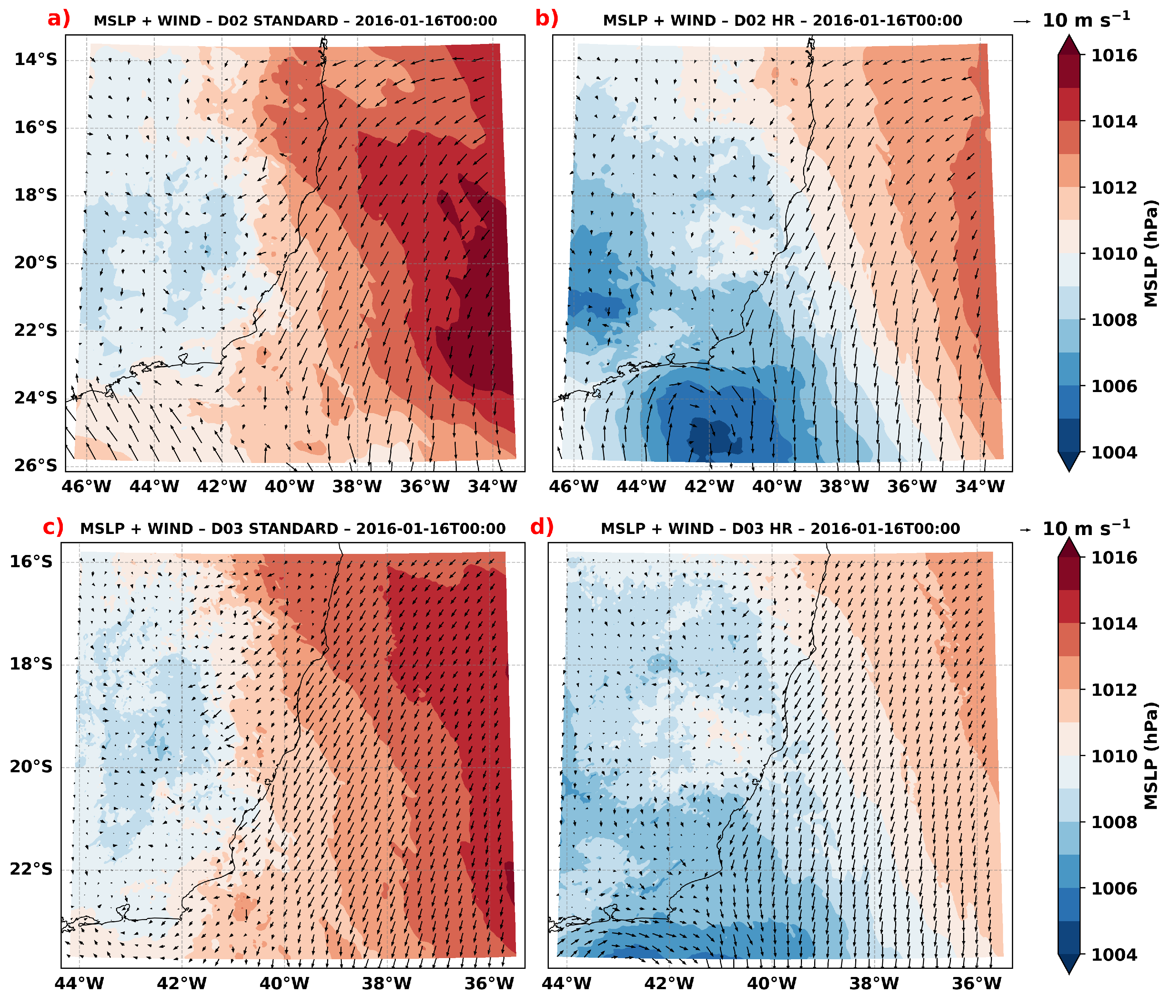
In Figure Figure 7, we observe the wind and mean sea-level pressure (MSLP) fields for domain d02, with panels (a) and (b) representing the WRF-GFS and WRF-RTG simulations, respectively. In panel (a), the wind field exhibits relatively weaker winds compared to panel (b), where the winds are stronger near the coast, particularly to the north, between 20° S and 24° S. Although no clearly defined low-pressure center is visible, the increased wind intensity along the coastal areas suggests a possible convergence of winds, which may be associated with an atmospheric convergence pattern.
At the intermediate resolution (D02), the atmospheric response to SST differences becomes more apparent in coastal regions (Figure 7). While no clearly defined low-pressure center is visible at this scale, significant differences in wind intensity are observed along the coastline. The high-resolution experiment (Figure 7b) shows enhanced wind speeds, particularly between 20°S and 24°S.
For domain d03, as shown in Figure Figure 7c-d, the wind analysis also reveals interesting dynamics. Although no clear low-pressure center is observed as in d01, areas of higher wind intensity are still present, particularly around 23° S near the coast. In panel (d), the winds are stronger compared to panel (c), suggesting that the inclusion of the higher-resolution RTG SST helps to better capture the wind intensity, especially in coastal regions.
These results demonstrate that the implementation of high-resolution SST data enables the model to capture mesoscale atmospheric features that are absent when using smoothed SST fields. The enhanced representation of thermal gradients leads to more realistic surface heat flux patterns, improved boundary layer dynamics, and consequently better representation of surface wind fields. This is particularly important in coastal upwelling regions where SST gradients can be extremely sharp and play a vital role in driving local atmospheric circulation patterns.
5. Conclusion
This study investigated the impact of SST resolution on atmospheric simulations over the southwestern Atlantic Ocean using the WRF model. Through comprehensive comparison of standard resolution GFS SST data with high-resolution RTG-SST-HR boundary conditions, we demonstrated significant improvements in model performance and physical realism when detailed SST structure is properly represented. In practical terms, resolving mesoscale SST gradients (fronts and upwelling filaments) is directly reflected in lower near-surface stability and more realistic low-level winds in coastal corridors, which is the quantity of immediate relevance to marine guidance.
The quantitative evaluation against observational buoy data revealed systematic improvements in wind field simulations when high-resolution SST was implemented. The most substantial improvements were observed for the u-component (zonal wind), with RMSE reductions of up to 0.5 m/s and correlation coefficient improvements of approximately 0.1 across multiple validation sites. These improvements were particularly pronounced at locations strongly influenced by coastal upwelling processes, such as Vitória and Santos, where enhanced representation of thermal gradients directly improved atmospheric boundary layer simulation.
The spatial analysis of wind and pressure fields demonstrated that high-resolution SST data enables the capture of mesoscale atmospheric features that are absent when using smoothed SST fields. The improved representation of coastal upwelling patterns, thermal fronts, and oceanic mesoscale structures led to more realistic surface heat flux patterns and enhanced atmospheric circulation features. In particular, the study identified enhanced cyclone organization and intensification in regions known for extratropical cyclogenesis, highlighting the importance of accurate SST representation for synoptic-scale weather prediction. Operationally, these mesoscale corrections shift the position and intensity of coastal low-level jets and convergence lines that precondition hazardous wave growth and wind surges during cyclogenesis, thereby tightening uncertainty bounds in day-ahead marine guidance.
The results have important implications for operational weather forecasting and climate modeling in the southwestern Atlantic region. The demonstrated improvements in wind field representation are particularly relevant for maritime safety, offshore operations, and coastal management applications. Furthermore, the enhanced representation of air-sea interaction processes contributes to better understanding of regional climate dynamics and ocean-atmosphere coupling mechanisms.
From a broader scientific perspective, this study reinforces the critical importance of high-quality boundary conditions in numerical weather prediction. The findings demonstrate that investment in high-resolution observational systems and data assimilation techniques can yield substantial improvements in model performance, particularly in regions characterized by strong air-sea interactions and complex coastal oceanography.
Future research directions should include investigation of optimal SST resolution requirements for different applications, assessment of computational cost-benefit ratios for high-resolution SST implementation, and development of improved parameterizations that can better represent sub-grid scale SST variability in coarser resolution models. Additionally, extension of this methodology to other coastal upwelling regions and different atmospheric models would provide broader validation of these findings.
Author Contributions
Conceptualization, M.B.L.S., M.M.R.P., J.T.A.C.; methodology, M.B.L.S., M.M.R.P., J.T.A.C.; software, M.B.L.S., M.M.R.P.; validation, M.B.L.S., L.C.J., F.T.C.B., M.M.R.P.; formal analysis, M.B.L.S.; investigation, M.B.L.S.; resources, M.M.R.P., J.T.A.C.; data curation, M.B.L.S., L.C.J., and M.M.R.P.; writing—original draft preparation, M.B.L.S.; writing—review and editing, M.B.L.S., F.T.C.B., K.C.L., and L.C.J.; visualization, M.B.L.S., F.T.C.B., K.C.L., and L.C.J.; supervision, J.T.A.C., M.M.R.P.; project administration, M.M.R.P.; funding acquisition, M.M.R.P..
Acknowledgments
We express our gratitude to the Laboratory of Free Surface Flow Simulation (LABESUL) and the Laboratory of Renewable Energies (LEAL), both from the Federal University of Espírito Santo (UFES), for their technical support and infrastructure throughout this research. Additionally, we are grateful to the National Buoy Program (PNBOIA) of the Brazilian Navy for providing the observed data.
Conflicts of Interest
The authors declare no conflict of interest.
References
- Kayano, M.T.; Andreoli, R.V.; de Souza, R.F.A. Evolving anomalous SST patterns leading to ENSO extremes: Relations between the tropical Pacific and Atlantic Oceans and the influence on the South American rainfall. International Journal of Climatology 2011, 31. [CrossRef]
- Woodcock, A.H. Surface cooling and streaming in shallow fresh and salt waters. Journal of Marine Research 1941, pp. 153–161.
- Ewing, G.; Mcalister, E.D. On the thermal boundary layer of the ocean. Science 1960, 131. [CrossRef]
- Grassl, H. The dependence of the measured cool skin of the ocean on wind stress and total heat flux. Boundary-Layer Meteorology 1976, 10. [CrossRef]
- Stull, R.B. An introduction to boundary layer meteorology. An introduction to boundary layer meteorology 1988. [CrossRef]
- Pezzi, L.P.; Souza, R.B.; Farias, P.C.; Acevedo, O.; Miller, A.J. Air-sea interaction at the Southern Brazilian Continental Shelf: In situ observations. Journal of Geophysical Research: Oceans 2016, 121. [CrossRef]
- Wallace, J.M.; Mitchell, T.P.; Deser, C. The Influence of Sea-Surface Temperature on Surface Wind in the Eastern Equatorial Pacific: Seasonal and Interannual Variability. Journal of Climate 1989, 2. [CrossRef]
- Businger, J.A.; Shaw, W.J. The response of the marine boundary layer to mesoscale variations in sea-surface temperature. Dynamics of Atmospheres and Oceans 1984, 8. [CrossRef]
- Song, Q.; Hara, T.; Cornillon, P.; Friehe, C.A. A comparison between observations and MM5 simulations of the marine atmospheric boundary layer across a temperature front. Journal of Atmospheric and Oceanic Technology 2004, 21. [CrossRef]
- Lindzen, R.S.; Nigam, S. On the Role of Sea Surface Temperature Gradients in Forcing Low-Level Winds and Convergence in the Tropics. Journal of the Atmospheric Sciences 1987, 44. [CrossRef]
- Kushnir, Y. Interdecadal variations in North Atlantic sea surface temperature and associated atmospheric conditions. Journal of Climate 1994, 7. [CrossRef]
- Deser, C.; Blackmon, M.L. Surface climate variations over the North Atlantic Ocean during winter: 1900-1989. Journal of Climate 1993, 6. [CrossRef]
- Grötzner, A.; Latif, M.; Barnett, T.P. A decadal climate cycle in the north Atlantic Ocean as simulated by the ECHO coupled GCM. Journal of Climate 1998, 11. [CrossRef]
- Sun, D.Z.; Liu, Z. Dynamic ocean-atmosphere coupling: A thermostat for the tropics. Science 1996, 272. [CrossRef]
- Seo, H.; Miller, A.J.; Roads, J.O. The Scripps Coupled Ocean-Atmosphere Regional (SCOAR) Model, with applications in the eastern Pacific sector. Journal of Climate 2007, 20. [CrossRef]
- Smirnov, D.; Newman, M.; Alexander, M.A. Investigating the role of ocean-atmosphere coupling in the North Pacific ocean. Journal of Climate 2014, 27. [CrossRef]
- Robertson, A.W.; Mechoso, C.R.; Kim, Y.J. The influence of Atlantic sea surface temperature anomalies on the North Atlantic oscillation. Journal of Climate 2000, 13. [CrossRef]
- Cui, C.; Xu, L. The Mesoscale SST–Wind Coupling Characteristics in the Yellow Sea and East China Sea Based on Satellite Data and Their Feedback Effects on the Ocean. Journal of Marine Science and Engineering 2024, 12. [CrossRef]
- Mughal, M.O.; Singh, V.K.; Martilli, A.; Acero, J.A.; Norford, L.K. Sea surface temperature impacts on tropical urban environment: A WRF modelling investigation. Urban Climate 2025, 62, 102502. [CrossRef]
- Busquets, E.; Udina, M.; Bech, J.; Mercader, J. Sea surface temperature updating impacts on WRF simulations during a heatwave period. Atmospheric Research 2025, 326, 108230. [CrossRef]
- Wu, C.; Wang, N.; Zhao, Y.; Dong, X.; Huang, W. Enhancing coastal wind simulation in the WRF model: Updates in sea surface temperature and roughness length through dynamic boundary conditions. Dynamics of Atmospheres and Oceans 2025, 110, 101542. [CrossRef]
- Srinivas, C.V.; Mohan, G.M.; Rao, D.V.B.; Baskaran, R.; Venkatraman, B., Numerical Simulations with WRF to Study the Impact of Sea Surface Temperature on the Evolution of Tropical Cyclones Over Bay of Bengal. In Tropical Cyclone Activity over the North Indian Ocean; Mohapatra, M.; Bandyopadhyay, B.; Rathore, L., Eds.; Springer International Publishing: Cham, 2017; pp. 259–271. [CrossRef]
- Venegas, S.A.; Mysak, L.A.; Straub, D.N. Atmosphere-ocean coupled variability in the South Atlantic. Journal of Climate 1997, 10. [CrossRef]
- Ruiz-Barradas, A.; Carton, J.A.; Nigam, S. Structure of Interannual-to-Decadal climate variability in the tropical Atlantic sector. Journal of Climate 2000, 13. [CrossRef]
- Zheng, Y.; Bourassa, M.A.; Hughes, P. Influences of sea surface temperature gradients and surface roughness changes on the motion of surface oil: A simple idealized study. Journal of Applied Meteorology and Climatology 2013, 52. [CrossRef]
- Chelton, D.B.; Xie, S.P. Coupled ocean-atmosphere interaction at oceanic mesoscales. Oceanography 2010, 23. [CrossRef]
- Song, Q.; Chelton, D.B.; Esbensen, S.K.; Thum, N.; O’Neill, L.W. Coupling between sea surface temperature and low-level winds in mesoscale numerical models. Journal of Climate 2009, 22. [CrossRef]
- Perlin, N.; De Szoeke, S.P.; Chelton, D.B.; Samelson, R.M.; Skyllingstad, E.D.; O’neill, L.W. Modeling the atmospheric boundary layer wind response to mesoscale sea surface temperature perturbations. Monthly Weather Review 2014, 142. [CrossRef]
- Doyle, J.D.; Warner, T.T. The impact of the sea surface temperature resolution on mesoscale coastal processes during GALE IOP 2. Monthly Weather Review 1993, 121:2. [CrossRef]
- Stark, J.D.; Donlon, C.J.; Martin, M.J.; McCulloch, M.E. OSTIA: An operational, high resolution, real time, global sea surface temperature analysis system. In Proceedings of the OCEANS 2007 - Europe, 2007. [CrossRef]
- Chin, T.M.; Vazquez, J.; Armstrong, E. Algorithm Theoretical Basis Document: A multi-scale, high-resolution analysis of global sea surface temperature. Remote Sensing of Environment 2013. Version 1.3.
- Dragaud, I.C.D.V.; Soares da Silva, M.; Assad, L.P.d.F.; Cataldi, M.; Landau, L.; Elias, R.N.; Pimentel, L.C.G. The impact of SST on the wind and air temperature simulations: a case study for the coastal region of the Rio de Janeiro state. Meteorology and Atmospheric Physics 2019, 131. [CrossRef]
- Wang, C. Three-ocean interactions and climate variability: a review and perspective. Climate Dynamics 2019, 53, 5119–5136. [CrossRef]
- Nonaka, M.; Xie, S.P. Covariations of Sea Surface Temperature and Wind over the Kuroshio and Its Extension: Evidence for Ocean-to-Atmosphere Feedback. Journal of Climate 2003, 16, 1404–1413.
- O’neill, L.W.; Esbensen, S.K.; Thum, N.; Samelson, R.M.; Chelton, D.B. Dynamical analysis of the boundary layer and surface wind responses to mesoscale SST perturbations. Journal of Climate 2010, 23. [CrossRef]
- da Silveira, I.C.A.; Schmidt, A.C.K.; Campos, E.J.D.; de Godoi, S.S.; Ikeda, Y. A corrente do Brasil ao largo da costa leste brasileira. Revista Brasileira de Oceanografia 2000, 48. [CrossRef]
- Luko, C.; Silveira, I.; Simoes-Sousa, I.T.; Araujo, J.; Tandon, A. Revisiting the Atlantic South Equatorial Current. Journal of Geophysical Research: Oceans 2021, 126. [CrossRef]
- Stramma, L.; England, M. On the water masses and mean circulation of the South Atlantic Ocean. Journal of Geophysical Research: Oceans 1999, 104. [CrossRef]
- Schmid, C.; Schafer, H.; Podesta, G.; Zenk, W. The Vitoria eddy and its relation to the Brazil Current. Journal of Physical Oceanography 1995, 25. [CrossRef]
- Nimer, E. Climatologia do Brasil; Instituto Brasileiro de Geografia e Estatística. Rio de Janeiro-RJ, 1989; p. 421.
- Cavalcanti, I.F.A.; Ferreira, N.J.; Dias, M.A.F.; Justi da Silva, M.G.A. Tempo e Clima no Brasil; Editora: Oficina de Textos. 1ª edição, 2009.
- Pezzi, L.P.; Souza, R.B. Variabilidade de meso-escala e interação Oceano Atmosfera no Atlântico Sudoeste; São Paulo: Oficina de Textos, 2009; pp. 385–405.
- Gan, M.A.; Rao, V.B. Surface Cyclogenesis over South America. Monthly Weather Review 1991, 119, 1293 – 1302. [CrossRef]
- Sinclair, M.R. An Objective Cyclone Climatology for the Southern Hemisphere. Monthly Weather Review 1994, 122, 2239 – 2256. [CrossRef]
- da Silva, M.B.L.; de Souza, D.C.; Barreto, F.T.C.; Tecchio, R.; de Freitas Pimentel dos Anjos, R.; Gramcianinov, C.B.; de Camargo, R. Classification of synoptic weather patterns associated with extreme wave events in different regions of Western South Atlantic. Natural Hazards 2025, 121, 9853–9877. [CrossRef]
- Gramcianinov, C.; Campos, R.; Guedes Soares, C.; de Camargo, R. Extreme waves generated by cyclonic winds in the western portion of the South Atlantic Ocean. Ocean Engineering 2020, 213, 107745. [CrossRef]
- Tecchio, R.; de Souza, D.C.; da Silva, M.B.L.; de Oliveria Costa, M.C.; de Camargo, R.; Harari, J. Mean sea level, tidal components and surges in Guanabara Bay (Rio de Janeiro) from 1990 to 2021. International Journal of Climatology 2024, 44, 4629–4648, [https://rmets.onlinelibrary.wiley.com/doi/pdf/10.1002/joc.8600]. [CrossRef]
- Couto de Souza, D.; da Silva Dias, P.L.; Gramcianinov, C.B.; da Silva, M.B.L.; de Camargo, R. New perspectives on South Atlantic storm track through an automatic method for detecting extratropical cyclones’ lifecycle. International Journal of Climatology 2024, 44, 3568–3588, [https://rmets.onlinelibrary.wiley.com/doi/pdf/10.1002/joc.8539]. [CrossRef]
- Matos, P.P.O.; Lorenzzetti, J.A.; Pezzi, L.P.; Pereira, G. Estudo comparativo preliminar dos campos de temperatura da superfície do mar OSTIA e RTG-SST-HR para a costa SE Brasileira. Anais XIV Simpósio Brasileiro de Sensoriamento Remoto 2009, 42, 6571–6577.
- Hong, S.Y.; Kim, J.H.; Lim, J.o.; Dudhia, J. The WRF single moment microphysics scheme (WSM). Journal of the Korean Meteorological Society 2006, 42, 129–151.
- Janjic, Z.I. The step-mountain eta coordinate model: further developments of the convection, viscous sublayer, and turbulence closure schemes. Monthly Weather Review 1994, 122. [CrossRef]
- Hong, S.Y.; Dudhia, J.; Chen, S.H. A revised approach to ice microphysical processes for the bulk parameterization of clouds and precipitation. Monthly Weather Review 2004, 132. [CrossRef]
- Mlawer, E.J.; Taubman, S.J.; Brown, P.D.; Iacono, M.J.; Clough, S.A. Radiative transfer for inhomogeneous atmospheres: RRTM, a validated correlated-k model for the longwave. Journal of Geophysical Research Atmospheres 1997, 102. [CrossRef]
- Dudhia, J. Numerical study of convection observed during the Winter Monsoon Experiment using a mesoscale two-dimensional model. Journal of the Atmospheric Sciences 1989, 46. [CrossRef]
- Jiménez, P.A.; Dudhia, J.; González-Rouco, J.F.; Navarro, J.; Montávez, J.P.; García-Bustamante, E. A revised scheme for the WRF surface layer formulation. Monthly Weather Review 2012, 140. [CrossRef]
- Niu, G.Y.; Yang, Z.L.; Mitchell, K.E.; Chen, F.; Ek, M.B.; Barlage, M.; Kumar, A.; Manning, K.; Niyogi, D.; Rosero, E.; et al. The community Noah land surface model with multiparameterization options (Noah-MP): 1. Model description and evaluation with local-scale measurements. Journal of Geophysical Research Atmospheres 2011, 116. [CrossRef]
- Tewari, M.; Chen, F.; Wang, W.; Dudhia, J.; LeMone, M.A.; Mitchell, K.; Ek, M.; Gayno, G.; Wegiel, J.; Cuenca, R.H. Implementation and verification of the unified noah land surface model in the WRF model. In Proceedings of the Bulletin of the American Meteorological Society, 2004.
- Kain, J.S. The Kain–Fritsch convective parameterization: an update. Journal of Applied Meteorology 2004, 43, 170–181.
- Skamarock, W.C. Evaluating mesoscale NWP models using kinetic energy spectra. Monthly Weather Review 2004, 132, 3019–3032.
- Weisman, M.L.; Skamarock, W.C.; Klemp, J.B. The resolution dependence of explicitly modeled convective systems. Monthly Weather Review 1997, 125, 527–548.
- Hallak, R.; Pereira Filho, A.J. Metodologia para análise de desempenho de simulações de sistemas convectivos na região metropolitana de São Paulo com o modelo ARPS: sensibilidade a variações com os esquemas de advecção e assimilação de dados. Revista Brasileira de Meteorologia 2011, 26. [CrossRef]
- Paranhos, R.; Figueiredo Filho, D.B.; da Rocha, E.C.; Silva Júnior, J.A.D.; Neves, J.A.B.; Santos, M.L.W.D. Desvendando os Mistérios do Coeficiente de Correlação de Pearson: o Retorno. Leviathan (São Paulo) 2014. [CrossRef]
- Xie, B.; Fung, J.C.H.; Chan, A.; Lau, A. Evaluation of nonlocal and local planetary boundary layer schemes in the WRF model. Journal of Geophysical Research: Atmospheres 2012, 117, [https://agupubs.onlinelibrary.wiley.com/doi/pdf/10.1029/2011JD017080]. [CrossRef]
- Nottrott, A.; Kleissl, J.; Keeling, R. Modeling passive scalar dispersion in the atmospheric boundary layer with WRF large-eddy simulation. Atmospheric Environment 2014, 82, 172–182. [CrossRef]
- Reboita, M.S.; da Rocha, R.P.; Ambrizzi, T.; Sugahara, S. South Atlantic Ocean cyclogenesis climatology simulated by regional climate model (RegCM3). Climate Dynamics 2010. [CrossRef]
Figure 1.
Study Area
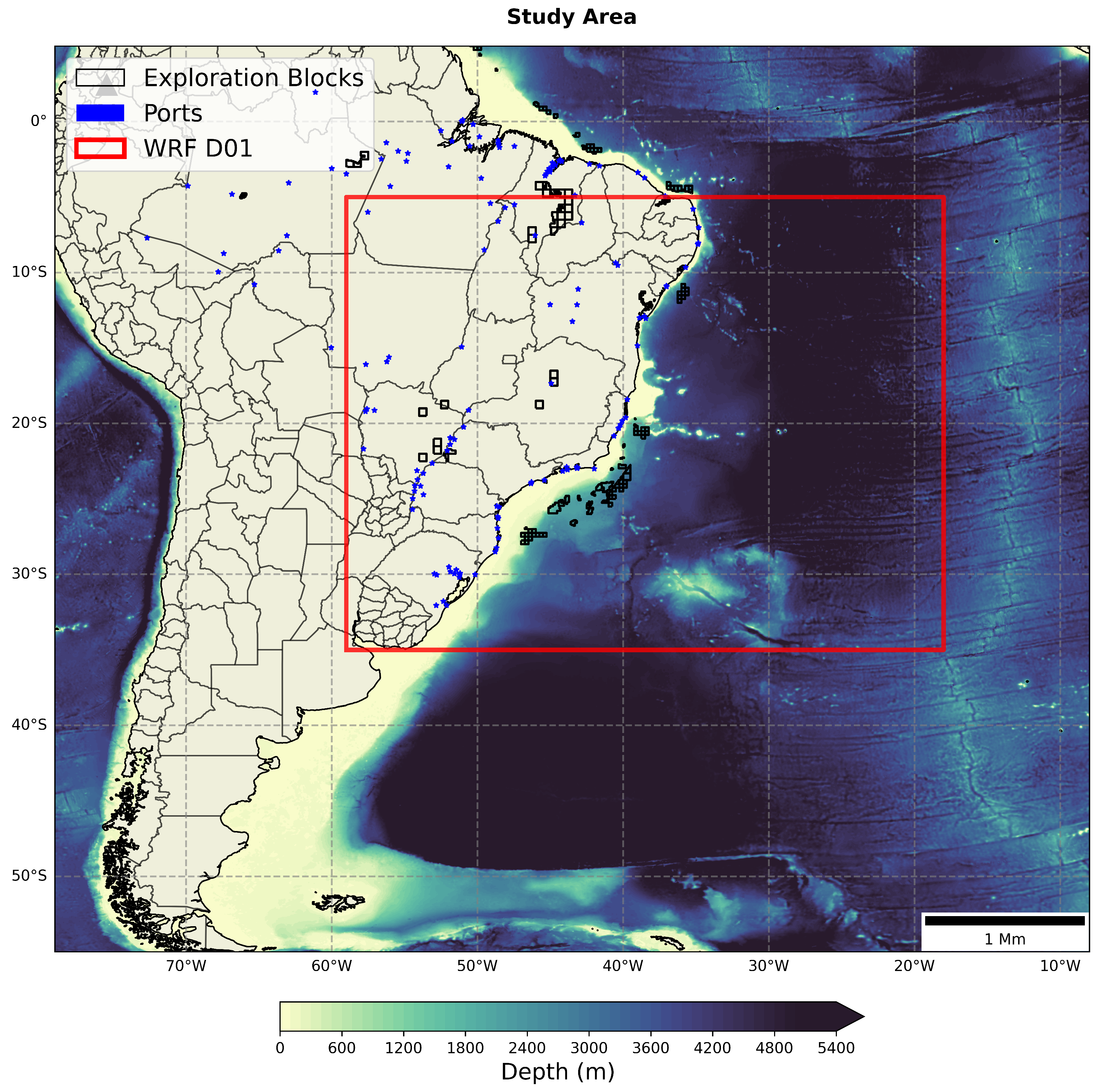
Figure 2.
Grid nesting used in WRF simulations
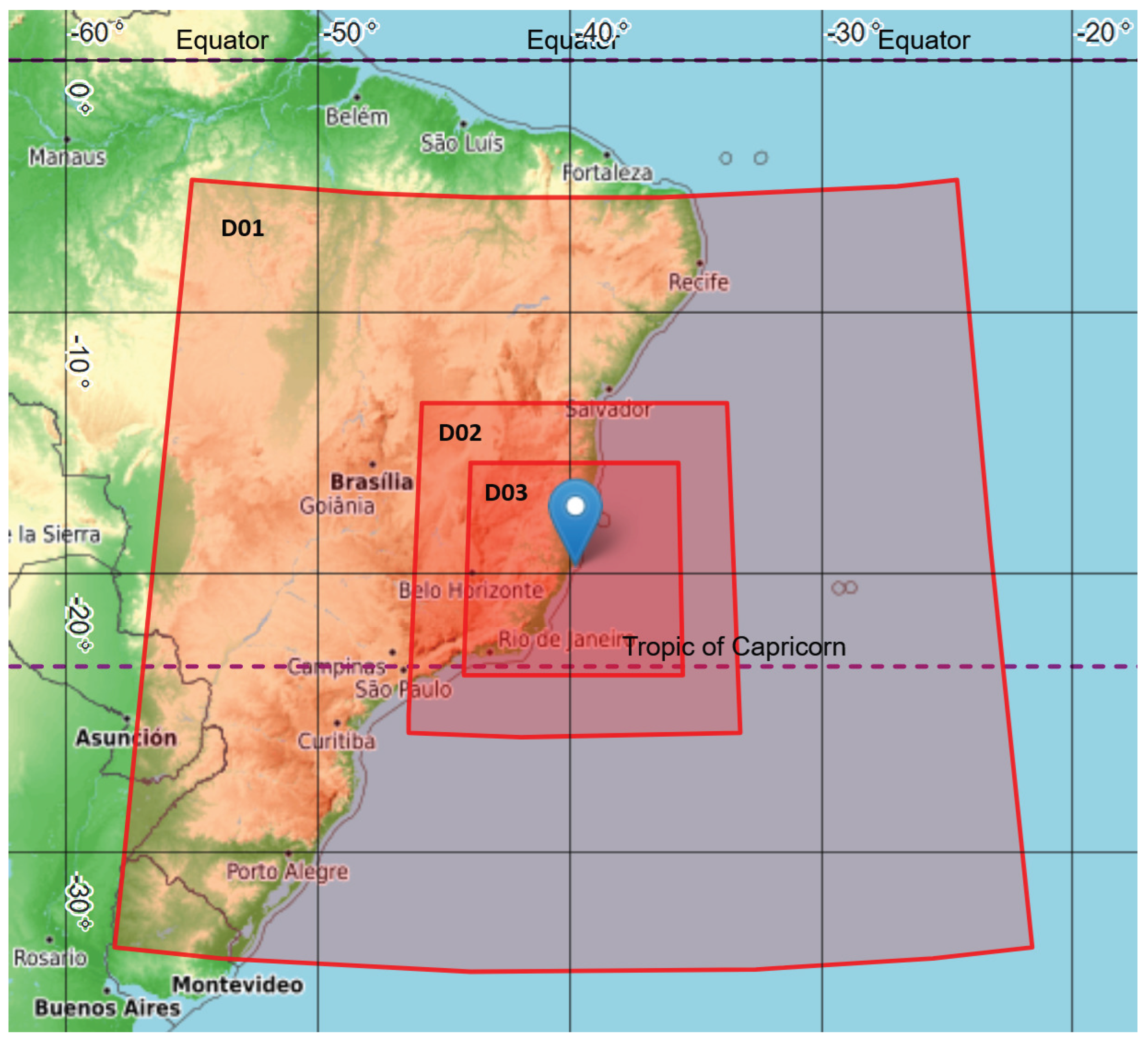
Figure 3.
Buoy locations used for validation and WRF domain hierarchy.Colored boxes delineate domains D01 (blue), D02 (red), and D03 (orange). Symbols denote individual buoys by domain, as indicated in the legend.
Figure 3.
Buoy locations used for validation and WRF domain hierarchy.Colored boxes delineate domains D01 (blue), D02 (red), and D03 (orange). Symbols denote individual buoys by domain, as indicated in the legend.
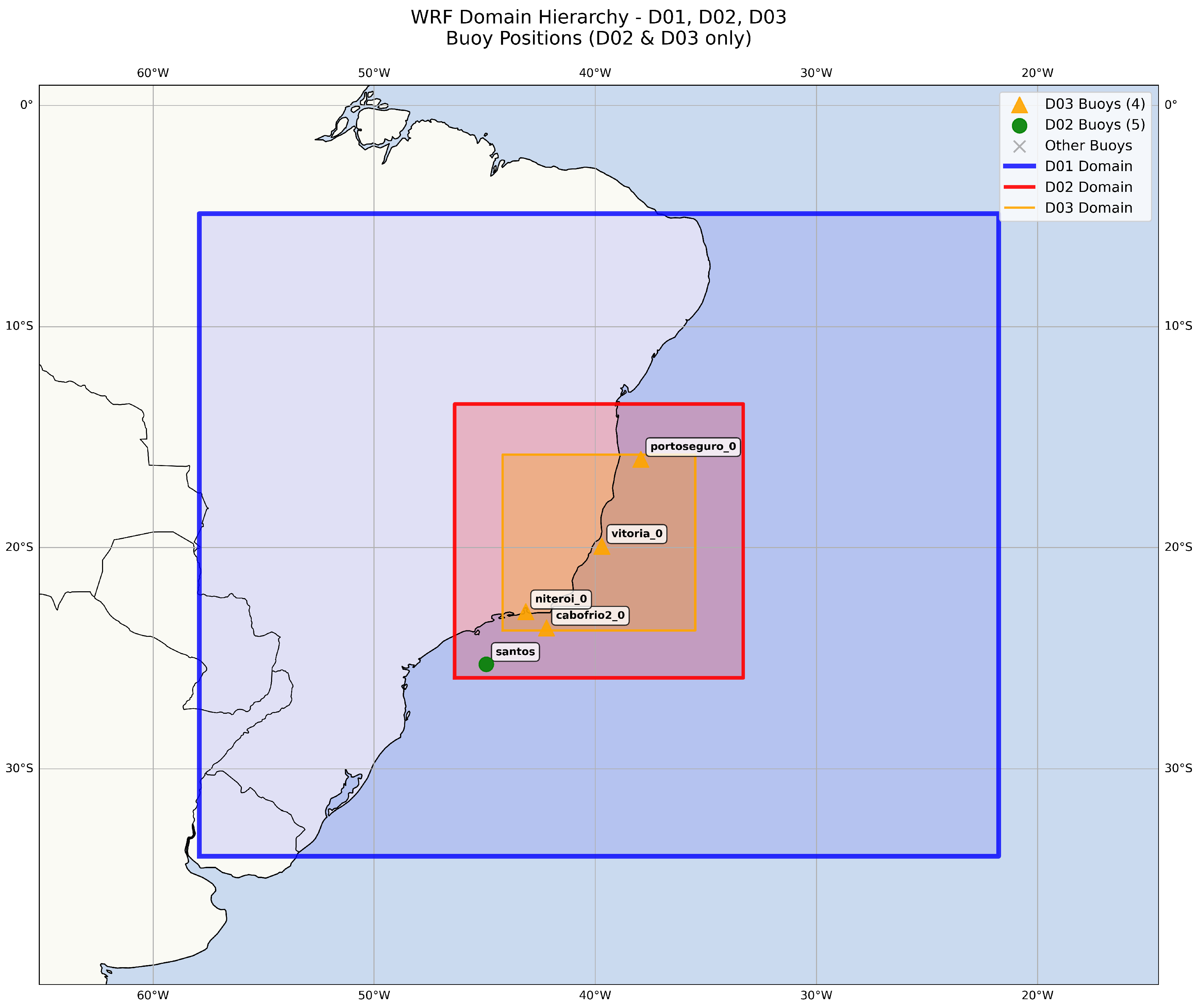
Figure 4.
Domain d01 on 16 January 2016 at 00:00 UTC. Panels show (a) 10 m wind and mean sea-level pressure (MSLP) from WRF-STD; (b) 10 m wind and MSLP from WRF-HR; (c) sea-surface temperature (SST) from GFS; and (d) SST from RTG.
Figure 4.
Domain d01 on 16 January 2016 at 00:00 UTC. Panels show (a) 10 m wind and mean sea-level pressure (MSLP) from WRF-STD; (b) 10 m wind and MSLP from WRF-HR; (c) sea-surface temperature (SST) from GFS; and (d) SST from RTG.
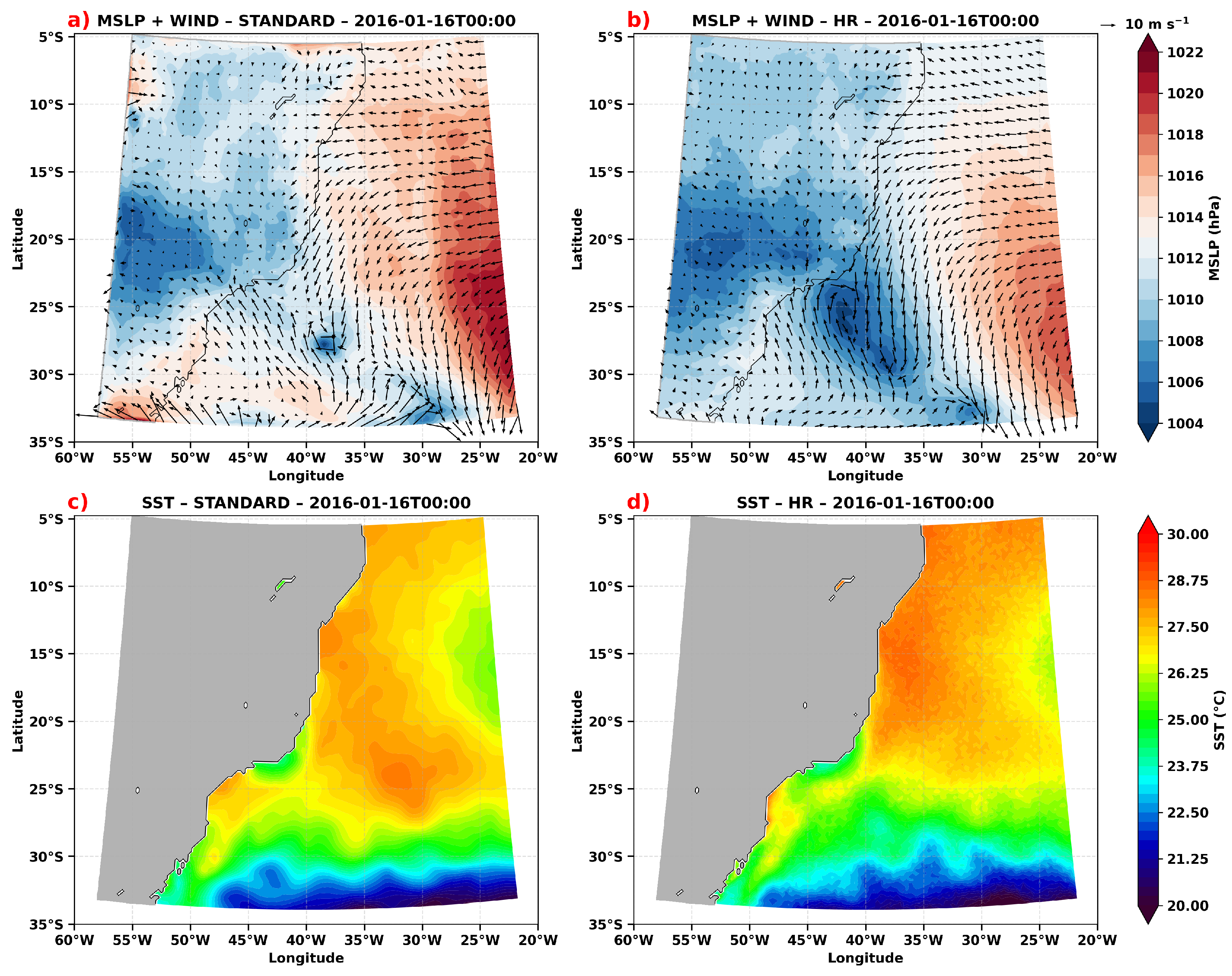
Figure 5.
ERA5 Reanalysis - Wind 10 meters and MSLP at 16/01/2016 - 00:00 UTC
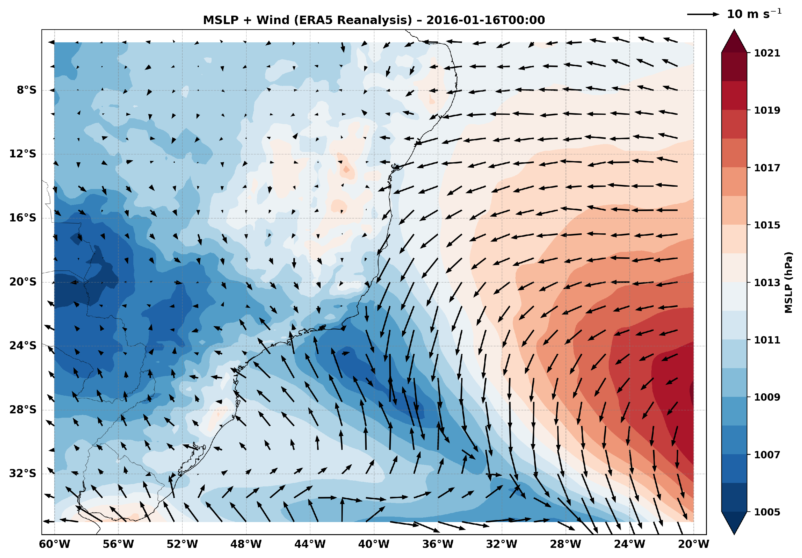
Figure 6.
Temporal RMSE and Pearson correlation of mean sea-level pressure (MSLP) between WRF simulations and ERA5 reanalysis for January 2016. Panels (a–b) correspond to the WRF simulation forced with the standard GFS SST (WRF-STD), while panels (c–d) correspond to the simulation forced with high-resolution SST fields (WRF-SST-HR). Panels (a,c) show the root-mean-square error (RMSE, hPa) computed over the entire month, and panels (b,d) show the temporal Pearson correlation coefficient between modeled and ERA5 MSLP at each grid point.
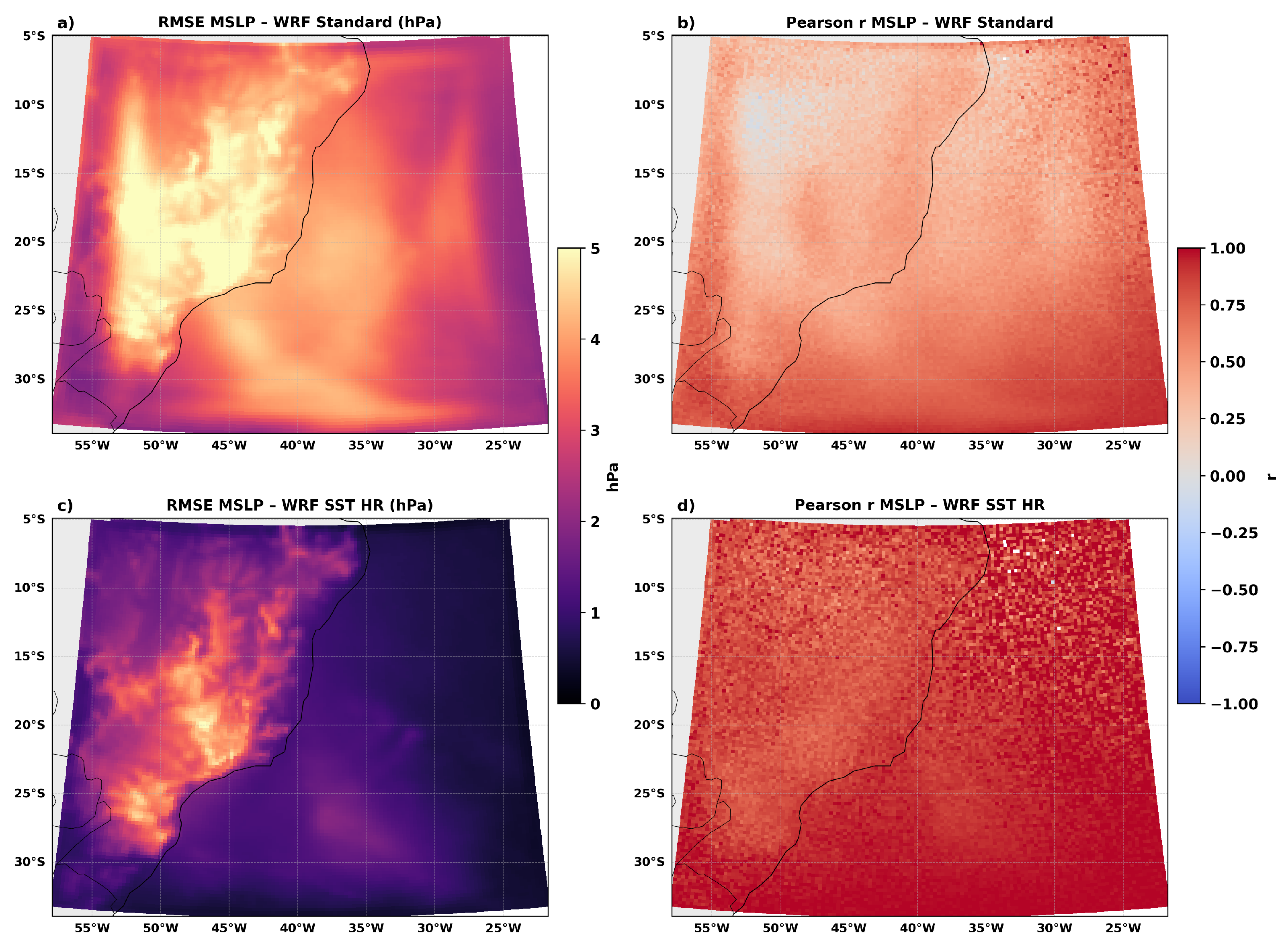
Figure 7.
Domain d02 and d03 on 16 January 2016 at 00:00 UTC. Panels show 10 m wind and MSLP from WRF (a) D02 Standard, (b) D02 SST HR ,(c) D03 Standard, and (d) D03 SST HR.
Figure 7.
Domain d02 and d03 on 16 January 2016 at 00:00 UTC. Panels show 10 m wind and MSLP from WRF (a) D02 Standard, (b) D02 SST HR ,(c) D03 Standard, and (d) D03 SST HR.
Disclaimer/Publisher’s Note: The statements, opinions and data contained in all publications are solely those of the individual author(s) and contributor(s) and not of MDPI and/or the editor(s). MDPI and/or the editor(s) disclaim responsibility for any injury to people or property resulting from any ideas, methods, instructions or products referred to in the content. |
© 2025 by the authors. Licensee MDPI, Basel, Switzerland. This article is an open access article distributed under the terms and conditions of the Creative Commons Attribution (CC BY) license (http://creativecommons.org/licenses/by/4.0/).
Copyright: This open access article is published under a Creative Commons CC BY 4.0 license, which permit the free download, distribution, and reuse, provided that the author and preprint are cited in any reuse.


