
Submitted:
24 September 2025
Posted:
25 September 2025
You are already at the latest version
Abstract
Sea surface temperature (SST) gradients modulate surface wind variability at the mesoscale O(100 km), with relevant impacts on surface fluxes, rainfall, cloudiness and storms. The dependence of the SST-wind coupling mechanisms on environmental conditions has been proven using global ERA5 reanalysis data. However, recent literature calls for the need of an observational confirmation to overcome the limitations of numerical models in representing such turbulent processes. Here, we employ O(10 km) MetOp A observations of surface wind and SST to verify the dependence of the downward momentum mixing (DMM) mechanism on large-scale wind U and atmospheric stability. We propose a simple empirical model describing the scaling of the coupling intensity on U, accounting for the role of the characteristic SST length scale LSST and the boundary layer height h in determining the decoupling of the atmospheric response from the SST forcing due to advection. Fitting such a model to the observations we retrieve a scaling with U that depends on the atmospheric stability, in agreement with the literature. The physical interpretation from ERA5 is confirmed, albeit relevant discrepancies emerge in stable regimes and specific regional contexts. This suggests that global numerical models are not able to properly reproduce the coupling in certain conditions, which might have important implication on air-sea fluxes.
Keywords:
space-borne earth observations
; air-sea interactions
; mesoscale
; numerical models
1. Introduction
Air-sea interactions play a crucial role in the transfer of heat, moisture, and momentum at the ocean-atmosphere interface. In the 1990s, monthly estimates of surface heat fluxes at 1°x1° resolution from optical and infrared observations of clouds and microwave radiometers showed surface wind is one of the major regulators of sea surface temperature (SST) due to its role in enhancing evaporative cooling and mixing with subsurface waters [1]. These findings confirm the leading role of the atmosphere in driving the ocean variability at the basin scale, i.e. at scales larger than 1000 km [2].
In the last two decades, the availability of high-resolution O(10) km scatterometer, radiometer and O(100) m SAR satellite observations has given a strong impulse to the study of air-sea interactions at smaller scales. Since then, relevant fine-scale interactions between the ocean mixed layer, the marine atmospheric boundary layer (MABL), and the free troposphere have been observed globally or investigated with numerical models [2,3,4,5]. Opposite to what we observe at the basin scale, fine-scale analyses show a predominant role of the ocean features in driving the atmospheric variability [6]. At the oceanic mesoscales, corresponding to horizontal scales of O(100-1000) km and weekly to monthly timescales, SST fronts, eddies, and oceanic currents have been observed to induce a tropospheric response with important weather and climate impacts [3,7]. Studies conducted over western boundary currents (WBCs) highlight a strong climatological response of tropospheric wind, clouds and rainfall to sharp SST fronts [8,9,10], while oceanic eddies contribute substantially to the net heat exchange between the atmosphere and the ocean [11,12]. Strong SST gradients also play an important role in storm development and intensification at daily scales [13,14]. Simulations and observations of air-sea interactions at the submesoscales O(1-100) km suggest a behaviour similar to that observed at the mesoscales [15,16,17] with notable differences related to the entanglement of different processes [18] and their strengths [19]. In particular, the systematic assessment of the intensity of such interactions and their feedback on larger scales is an active area of research [20].
Mesoscale air-sea interactions encompass various processes, usually divided into thermal (TFBs) and current (CFBs) feedbacks, which describe the influence of SST and ocean currents on the MABL. In the case of CFBs, the relative motion between the surface wind and the current generates a wind stress anomaly, increasing the momentum transfer from the ocean to the atmosphere [21,22]. As a main consequence, this mechanism acts as an “eddy killer”, with relevant effects on the kinetic energy repartition in the ocean. Mesoscale currents, being mostly geostrophic, do not exhibit a relevant divergence, and therefore they only induce a response in surface wind curl, allowing for a decoupling from TFBs acting on surface wind divergence [23].
Within TFBs, the main mechanisms explaining wind-SST coupling are downward momentum mixing (DMM) [24,25] and pressure adjustment (PA) [26]. DMM consists of an increased transport of momentum from the free troposphere to the surface due to enhanced mixing when passing from colder to warmer SST. This atmospheric mixing is enhanced by the increasing heat turbulent fluxes in the transition, resulting in the deepening of the MABL due to the entrainment of free tropospheric air, which results in higher surface wind and a weaker wind at the MABL top [27]. According to the PA mechanism, a negative (positive) surface pressure anomaly develops over a warm (cold) SST anomaly due to the increased (decreased) sensible heat flux. The related pressure gradient induces a secondary circulation exhibiting surface wind convergence (divergence) over the SST anomaly. The intensity of the TFB mechanisms is usually measured with coupling coefficients, which are the linear slope of the binned scatterplot of relevant fields. For instance, for DMM, the SST gradient and the surface wind divergence are considered, whereas for PA the SST Laplacian and the surface wind divergence are analyzed [2,3,7,28,29].
Studies comparing SST-wind coupling coefficients from satellite observations and from high-resolution numerical simulations show large discrepancies, both for atmospheric [23,30] and for ocean-atmosphere coupled models [31]. This can be related to parametrization of unresolved processes, as demonstrated by the dependence of the coupling coefficients on the choice of the MABL turbulent scheme [32,33], and indicates that models still struggle in properly representing air-sea interactions, possibly influencing long-standing biases in global models [34]. The analysis of air-sea interactions from observational data is thus useful both to characterize the processes at play and to guide the development of revised numerical schemes.
Instantaneous and daily scatterometer and radiometer observations have shown a significantly larger value of DMM coupling coefficient with respect to that obtained from multi-annual and monthly data over the Gulf Stream [3,7,35]. Similar results have been found both at the mesoscale and at the submesoscale, and they suggest that SST-wind coupling is active at very short, sub-daily timescales [15,16,36].
Regional factors, via different environmental properties, also play a role in modulating the coupling intensity [7,37,38]. For example, the coupling strength has been shown to depend on the scale of motion and on the Rossby number, as they directly affect the advective timescale and the characteristic length of the SST features[39].
Large-scale wind speed and atmospheric stability are also important drivers of DMM and PA coupling intensity [38]. In addition to its contribution to advection, large-scale wind is related to the free tropospheric wind, which powers DMM, while atmospheric stability regulates the development of the vertical motion, which is instrumental for both DMM and PA [37,38,39]. These relationships have been described starting from the analysis of numerical simulations and of global reanalysis data, that present systematic biases in surface wind compared to scatterometer observations [34,40,41,42] and in MABL humidity, temperature and surface heat fluxes [16,43,44,45]. A corresponding analysis based on remote sensing data, that is still missing, would corroborate their physical interpretation.
Here, our objective is twofold: (1) to provide a global observational assessment of the environmental control of large-scale wind and atmospheric instability on the intensity of the DMM coupling following Desbiolles et al. (2023) [38], and (2) to verify how much of the physical interpretation based on the reanalysis and the observational global datasets translates at the regional level, and which additional factors could be responsible for uncaptured variability of the DMM coupling emerging in regional contexts. Section 2 describes the data and methods used, while results are presented in Section 3. Section 4 is devoted to a final discussion.
2. Materials and Methods
2.1. Datasets
The observational analysis covers the period between January 2020 and October 2021. SST data come from the Advanced Very High Resolution Radiometer (AVHRR) instrument onboard of MetOp-A, distributed as part of the ESA-CCI dataset. In particular, we make use of the L3C (Level 3 Collated) product v2.1 obtained from Copernicus Climate Change Service (C3S) Climate Data Store (CDS) platform [46]. It consists of instantaneous SST observations provided as global maps, collecting all orbits on a 0.05° latitude-longitude regular grid, separated between night-time and day-time acquisitions. The data are not available in the presence of sea ice and clouds, which strongly reduce the coverage in regions with high cloud cover and polar regions. Quality flags are attributed to the data representing their reliability depending on the known causes of uncertainties in the processing, such as dust and thin clouds. Following Merchant et al. (2019) [47], all data with a quality flag of 3 or higher are considered reliable for the computation of gradients and anomalies for our analyses.
Surface wind observations consist of the L2 coastal product derived from MetOp-A Advanced Scatterometer (ASCAT) Climate Data Record (CDR) dataset [48]. They are available on the NASA JPL-PODAAC platform in the format of single orbit files containing instantaneous observations of the two 550 km swaths on a 12.5 km irregular grid, following the satellite track projection on the surface. The data are also quality-flagged based on their reliability, with rainfall and extremely low or high values of wind speed as the main known sources of uncertainty. We remove all the points with high uncertainty (quality flag higher than ) to ensure the reliability of the analysis.
Atmospheric stability is here defined using air-sea temperature difference () as a proxy [38,49], given that it regulates surface heat fluxes, and therefore the buoyancy flux and air-column stability. Clearly, other factors such as moisture and subsidence influence stability but will not be considered here. Negative (positive) values of air-sea temperature differences correspond to a warm (cold) ocean heating (cooling) the overlying atmosphere, favouring (inhibiting) vertical transport due to the enhanced (reduced) buoyancy and air-column instability. As no satellite observations of air temperature data with suitable coverage and resolution are currently available, to estimate the air-sea temperature difference we use hourly data of 2m air temperature and SST, collocated with MetOp observations, from the ERA5 product. ERA5 is a global reanalysis describing the atmosphere, land surface and ocean surface produced by the European Centre for Medium-Range Weather Forecasts (ECMWF) and distributed through the CDS portal [44]. The data are on a regular grid at 0.25° horizontal spacing and hourly frequency. The model assimilates a wide set of satellite and in-situ observations, making it a reference dataset for climate studies.
From ERA5, we also take daily fields of 10m wind, SST, and 2m air temperature to reproduce the analyses from Desbiolles et al. (2023) in the time window between January 2000 and December 2021.
2.2. Data analysis and coupling metrics
We aim to compute the DMM coupling coefficients as a function of the large scale wind and the air stability defined as the air-sea temperature difference. To do so, a few pre-processing steps are needed. Following the methodology of Meroni et al. (2023) [35], SST data are smoothed through a Gaussian filter with a standard deviation of 10 km to reduce the noise and remove the fine-scale variability that is not captured by the wind product, being it on a coarser grid. Wind data are interpolated on the finer SST regular grid using a bilinear interpolation. This is meant to preserve the full range of variability of SST gradients and has the effect of repeating wind divergence values over contiguous pixels. A 50 km coastal mask is applied to all datasets to remove coastal effects such as land-sea breeze and orographic effects, and to ensure the scatterometer observations are not affected by land scattering.
A two-dimensional Gaussian low-pass filter is then applied to the surface wind field to estimate its large-scale component and, from that, the mesoscale anomaly . This anomaly can be decomposed on a local Cartesian frame of reference , with r being the along- direction and s the across- direction (positive at 90° counterclockwise to r), so that
as in [50].
The standard deviation of the Gaussian filter is defined differently depending on the wind field product considered. For ERA5 wind, km, which provides a smoothing comparable to the 1000 km Lanczos filter used in Desbiolles et al. (2023) [38]. For ASCAT wind, instead, km, as in Meroni et al. (2022, 2023) [35,50]. Sensitivity analyses for applied to both wind products ( km for ERA5 and km for ASCAT) indicate that results have a negligible dependence on it, for reasons that are discussed later in the manuscript.
From the SST and fields, centered finite-difference spatial derivatives are computed to obtain the along-wind SST gradient and the along-wind wind divergence . Following Meroni et al. (2023) [35], the DMM coupling coefficient is defined as the slope of the linear regression between these two fields, as in
As most of the SST gradients fall into a narrow interval corresponding to weak SST gradients, in fact sharp SST features are rare across the ocean, a weighted linear regression is applied to the uniformly binned SST gradient distribution. We define 20 bins of and for each of them we compute the mean SST gradient, the mean wind divergence, and its standard error (defined as the ratio between the standard deviation and the square root of the number of values in the bin). The standard error is used as a weight in the least-square linear regression, as in "Numerical Recipes", Chapter 15.2, Eq. 15.2.6 [51]. The uncertainty of each coupling coefficient is estimated through the square root of slope variance according to "Numerical Recipes", Chapter 15.2, Equation 15.2.9 [51]. This approach ensures a uniform coverage of the SST gradient distribution while emphasizing the most reliable bins.
To increase the robustness of the fit, bins containing fewer than 100 points are excluded, and we reject all cases where more than 50% of the bins are absent. This is to reduce noisy data and ensure that the linear regression is not performed on very few bins. Furthermore, cases where the coefficient of determination () of the least-squares regression falls below 0.8 are also discarded. This eliminates cases that would make the estimate of the coupling coefficients unreliable, such as cases where the slope shifts sign between positive and negative SST gradients. For each region and product, a different binning of the SST gradient distribution is defined to cover its full range. This is needed because we compare subsets with very different ranges of SST gradients, partially due to the presence or not of sharp SST features (e.g. WBCs), and partially because of the variability of the Rossby radius of deformation with latitude, which may indirectly affect the SST gradient strength.
The coupling coefficients are computed over subsets of data grouped by the values of their large-scale conditions. Classes of large-scale wind speed U range from 0 m/s to 24 m/s, with a sampling frequency of 2 m/s, while classes of air stability range from -16 K to 6 K, sampled every 2 K.
We tested the methodologies of Meroni et al. (2023) and Desbiolles et al. (2023) against the methodology proposed here to evaluate its potential biases. The tests showed that the exact value of the coupling coefficient is sensitive to the precise methodology used to compute it (we obtained values 30% smaller than the one in Meroni et al. (2023), and 40% larger than in Desbiolles et al. (2023)), but the dependence on environmental conditions is not affected.
2.3. Regions of interest
Regional analyses are carried out over the regions reported in Figure 1. WBCs regions (namely Gulf Stream, Agulhas, Malvinas, and Kuroshio) are rich in mesoscale SST features and present very sharp SST gradients, in the order of 1 K/10 km. They are characterised by strong westerly winds and a wide range of atmospheric stability conditions, varying from marginally stable ( K) to very unstable ( K). Strong instability often develops during the cold season, when cold air outbreaks (CAOs) bring cold air masses from the continental plains over the Gulf Stream and the Kuroshio current [52]. Tropical areas, such as the EUREC4A region near Barbados (where the EUREC4A, ElUcidating the RolE of Cloud–Circulation Coupling in ClimAte, field campaign took place) [53] and the Benguela current along the coasts of Namibia and Angola, present mostly marginally unstable to marginally stable conditions ([-5 K; 3 K]), with weaker winds and mild SST gradients.
Global analyses are also performed, employing data between -60° and 60° latitudes to reduce the impact of sea ice and ensure the comparability with Desbiolles et al. (2023) [38].
3. Results
3.1. Global analysis of coupling dependence on environmental conditions
Global reanalysis data and regional observations have highlighted the dependence of the DMM coupling coefficients on environmental conditions such as large-scale wind speed, atmospheric instability and Rossby number [38,39]. Here, we present a framework to interpret those dependencies, we investigate if the same results are confirmed by global observations and if any discrepancy from the global analyses emerges at the regional level for both observational and reanalysis data.
We consider that the atmospheric response to underlying SST patterns is controlled by the ratio between two timescales [38]: the advective timescale
where is a representative length scale of the SST feature, and the time scale of the DMM response
considered to be proportional to the boundary layer height h. Whenever the response time scale is short compared to the advective time scale, the imprint of the SST patterns will manifest in the near-surface winds. Conversely, for long compared to the boundary layer properties will not have the time to fully adjust to the underlying SST before the air moves away from the SST feature, and the response will be weak. In relation to the environmental conditions introduced above, we note that the boundary layer height depends on air column stability and on wind speed [54,55], and that the spatial scale of the SST structures is related to the Rossby number.
This framework allows us to discuss the dependence of the coupling coefficient on large scale wind U, that shows, both for the observational and for the reanalysis datasets, an initial increase in coupling intensity followed by a peak and a subsequent decrease at larger U (Figure 2a). As a first approximation, we consider h to be independent of U, such that is considered constant. At low U, the advective timescale is large, resulting in . For increasing large-scale wind U, we postulate that also the free-tropospheric wind increases. Thus, the enhanced mixing over warm SST accelerates more the surface flow, hence increasing the atmospheric response at the surface and resulting in growing with U. At high enough U, however, , meaning that the lower atmosphere does not fully adjust to the SST forcing feature before being advected beyond it, leading to a weaker coupling. Peak coupling coefficients are hence obtained for , and the corresponding surface wind speed is
Despite the overall agreement between the sensitivity of the coupling coefficient on U in the observational and in the reanalysis datasets, important differences also emerge. For MetOp, is smaller than for ERA5. We argue that this is because SST features in MetOp observations exhibit sharper gradients than in ERA5, leading to smaller than those present in reanalysis, and resulting thus in a smaller . We bring this argument forward in the next section, where we develop an empirical model to further investigate this behaviour.
In terms of air stability, measured by , Figure 2b shows that for both datasets the largest coupling coefficient is obtained for neutral or marginally stable conditions ( [-1 K, 3 K]). As discussed in Desbiolles et al. (2023) [38], this is related to the fact that the near surface warming induced by SST features is too weak to destabilize the air-column in conditions of strong stability (large positive ) or provide a relevant contribution to the ongoing mixing occurring in unstable conditions (large negative ). The peak in the wind response to underlying SST features is thus obtained for values of close to zero. Despite the overall agreement between the sensitivity of the coupling coefficients on air-sea temperature difference obtained with observational and reanalysis data, a key difference between the two dataset emerges under marginally stable conditions ( K): while observations indicate a strong coupling, reanalysis display a large drop in coupling intensity. We interpret the strong coupling in MetOp for marginally stable conditions to be related to the shallow boundary layer that is typically characteristic of nighttime conditions and upwelling regions: sea surface temperature structures manifest in large changes in atmospheric properties, given the small air mass present in the boundary layer. Noting that numerical models strongly overestimate the depth of stable boundary layers, as they struggle to correctly represent mixing in the presence of weak and intermittent turbulence and are limited by their vertical resolution [56], our interpretation is also consistent with the smaller coupling coefficients obtained in ERA5 than in MetOp.
By considering the combined dependence of the coupling coefficient as a function of U and from the MetOp data, the first feature that emerges is that there is a much stronger dependence on the air stability than on the background wind speed (Figure 3a). Moreover, it can be noticed that is about 5 m/s for , and it increases to about 7 m/s for stable conditions (), where the boundary layer is expected to be shallower. This confirms the hypothesis described above on the leading role of h in determining both and the intensity of the atmospheric response to the SST forcing.
3.2. Regional characterization of air-sea coupling
Regional analyses performed on MetOp data over WBCs show strong similarity with the global analysis, suggesting that these regions contribute the most to the global behaviour (Figure 4 a,b). In fact, they display an increase in coupling strength for increasing wind speed, followed by a peak and a subsequent decrease (Figure 4a). In terms of air stability, they display an increase for marginally unstable conditions, followed by a sort of plateau for stable conditions (Figure 4b). The analyzed tropical areas, instead, provide different results. First, the value of is larger than for the WBCs. Then, in the Benguela region the coupling coefficients are larger, with exceptionally high coupling intensity obtained for marginally stable conditions. This is consistent with the fact that the colder waters of the Benguela upwelling system induce a shallow MABL [57], for which the SST forcing induces a strong response due to the smaller amount of air to be affected. The EUREC4A region shows strong non-linearities in its coupling curves (not shown), hindering the evaluation of the coupling through our linear metrics.
Considering ERA5 data, instead, unlike for MetOp, WBC curves as a function of U exhibit a wider spread and peak at different locations (Figure 4c). The lowest peak is found in the Agulhas Current, with m/s, whereas the Gulf Stream shows no decreasing tendency within the available U range. The computation of the coupling coefficient over the tropical region reveals numerous nonlinearities (not shown), resulting in the exclusion of a substantial portion of the data. Considering the remaining points, the EUREC4A region exhibits stronger coupling intensity than the observations, which is unexpected given the absence of fine-scale features in ERA5 [58], while the Benguela Current displays negative coupling values, in sharp disagreement with the physical understanding of DMM. Strong nonlinearities also affect the analysis of the influence on the coupling intensity, especially over the tropics, the Gulf Stream and the Kuroshio Current, while the remaining WBCs show a behaviour compatible with the MetOp data (Figure 4d).
Overall, this investigation indicates that observations lead to a more linear dependence between wind divergence and SST gradient than ERA5 data, and a more consistent dependence of on the environmental conditions. Instead, ERA5 data give rise to numerous nonlinearities and differences among the different geographical regions.
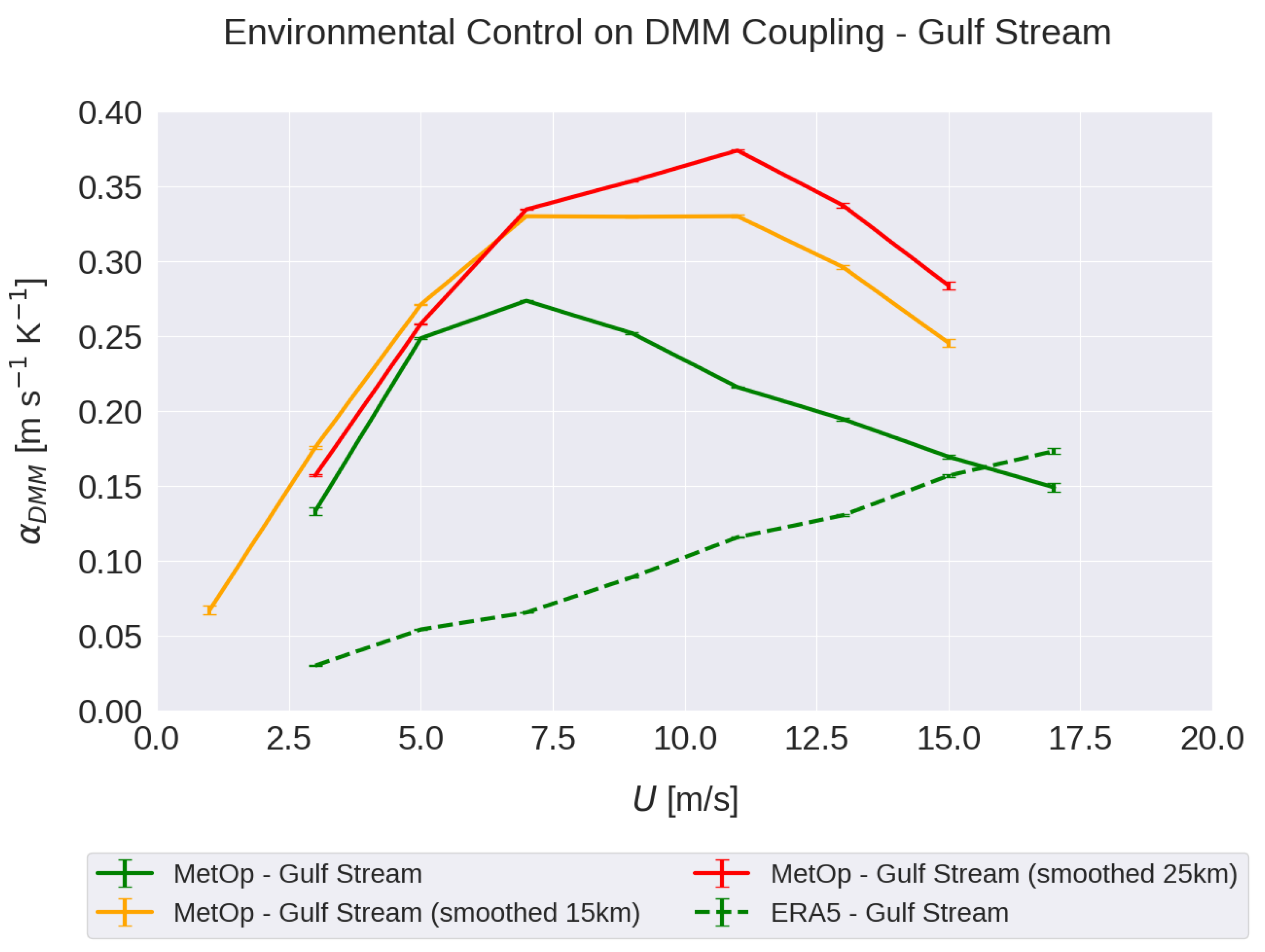
3.3. Dependence of coupling on SST structures spatial scale
We here verify that for larger length scale of the SST features, the peak coupling happens at larger U, as indicated by Equation 5. To this aim, we low pass filter MetOp data before computing the coupling coefficients, effectively reducing the SST and wind field resolution and therefore artificially increasing . Two Gaussian filters with standard deviation of 15 km and a 25 km have been used. The coupling coefficients computed on the smoothed data show respectively m/s and m/s, while it was m/s for the unfiltered (finer scale) data. This clearly indicates that increases with increasing .
This analysis also supports our interpretation of the larger obtained using ERA5 data, which resolves coarser SST features with respect to MetOp. Similarly, the difference in between mid-latitudes and tropical regions in Figure 4 is consistent with the fact that the SST features characteristic length decreases with latitude as the first baroclinic Rossby radius of deformation [59].
Figure 5.
DMM coupling coefficient as a function U over the Gulf Stream. Data corresponding to the original resolution (green, full line) and Gaussian-filter smoothed data (orange with km, red with km) are shown. The ERA5 corresponding curve (green, dashed line) is reported for comparison.
Figure 5.
DMM coupling coefficient as a function U over the Gulf Stream. Data corresponding to the original resolution (green, full line) and Gaussian-filter smoothed data (orange with km, red with km) are shown. The ERA5 corresponding curve (green, dashed line) is reported for comparison.
3.4. Empirical model for the large-scale wind dependence
The fact that the dependence of on U is non-monotonic for both ERA5 and MetOp data indicates its robustness. In its initial interpretation, brought forward by [38] and summarized above, the dependence on U only appears in the advective time scale . Here, by arguing that U also affects the response time scale , we develop a more comprehensive empirical model of as a function of U.
We hypothesize that DMM generates a surface wind anomaly with the following characteristics:
- (1)
- is a fraction of the large-scale wind U;
- (2)
- the ratio controls the efficiency of the process as an exponential decay.
Thus, we write
where represents the fraction of U that would be observed at the surface due to mixing in the case of an instantaneous atmospheric response (, so that ). Instead, for a very slow response, , the mixing is inefficient and no surface DMM wind anomaly is produced, so .
The value of can be thought as increasing for increasing surface instability, namely
where accounts for neutral conditions, and is a constant. Considering that to a leading order adjusts to SST, this can be recast in
With these assumptions, the DMM coupling coefficient estimated from the data can be expressed as
where represents the surface wind speed anomaly generated by other processes than DMM and
Drawing from the extensive literature on the scaling of the MABL height with surface fluxes and, thus, with the wind speed, we can model with according to different models, and as a function of the air stability [55,60,61]. From here,
with and c being a constant. This leads to
The simplified model for the coupling coefficient in Equation 13 captures the behaviour observed in the data: increases linearly with U for small U, it reaches a peak and then decays to zero as , assuming from the literature [55]. Moreover, if was independent of the environmental conditions, as proposed by Desbiolles et al. (2023) [38], we would have and there would be no decay for large U. This indicates that it is necessary to include a scaling of h with U to properly model the data.
Since Kitaigorodskii et al. show a different scaling of depending on stability [61], we treat stable () and unstable () conditions separately.
In unstable conditions, a possible scaling of h with U comes from , where B is the surface buoyancy flux [61], that scales as using a bulk formulation approach. Thus, for unstable conditions , so that and .
In stable conditions, instead,
with being the Obukhov length [54] and exploiting the scaling of the friction velocity . This leads to and .
Despite those scaling predict values for , we keep it as a free parameter in the model and use the data to empirically obtain its value, together with the values of and . The description of the fitting procedure is reported in Appendix A.
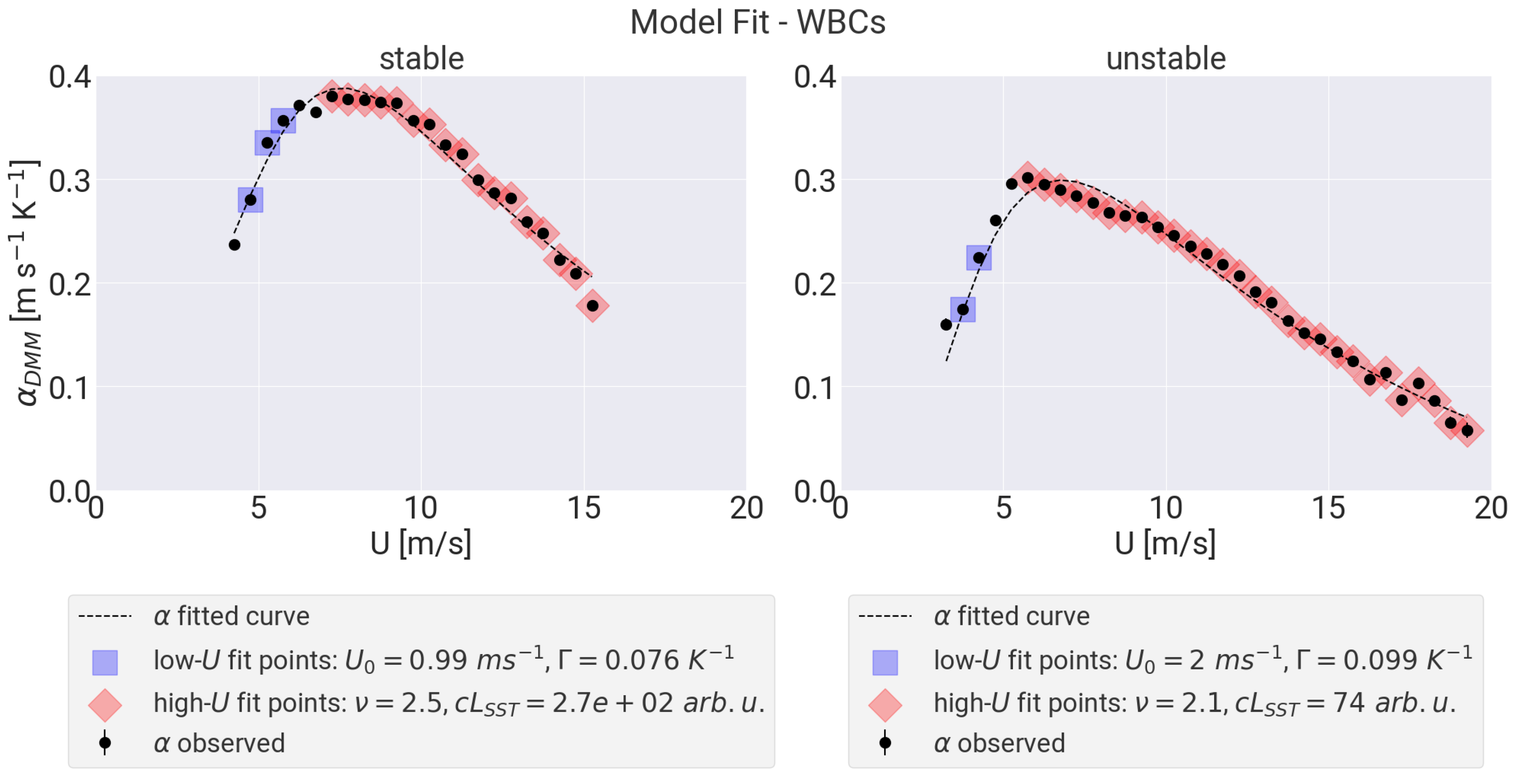
Assuming that the dynamic regimes and the statistics of are comparable over WBCs, we aggregate their data to increase the robustness of the results. Tropical regions present almost no data for to perform the fit, and therefore their analysis is not shown. The fit reasonably agrees with the observed data both in stable and unstable conditions (Figure 6). In particular, in both cases, the decay for large U is guaranteed by . From the fit of the aggregated WBCs data we obtain in unstable conditions, slightly overestimating the reference value , and in stable conditions, slightly underestimating the reference value , but coherent with other h scalings in the literature [55,60,62], as discussed in the next section.
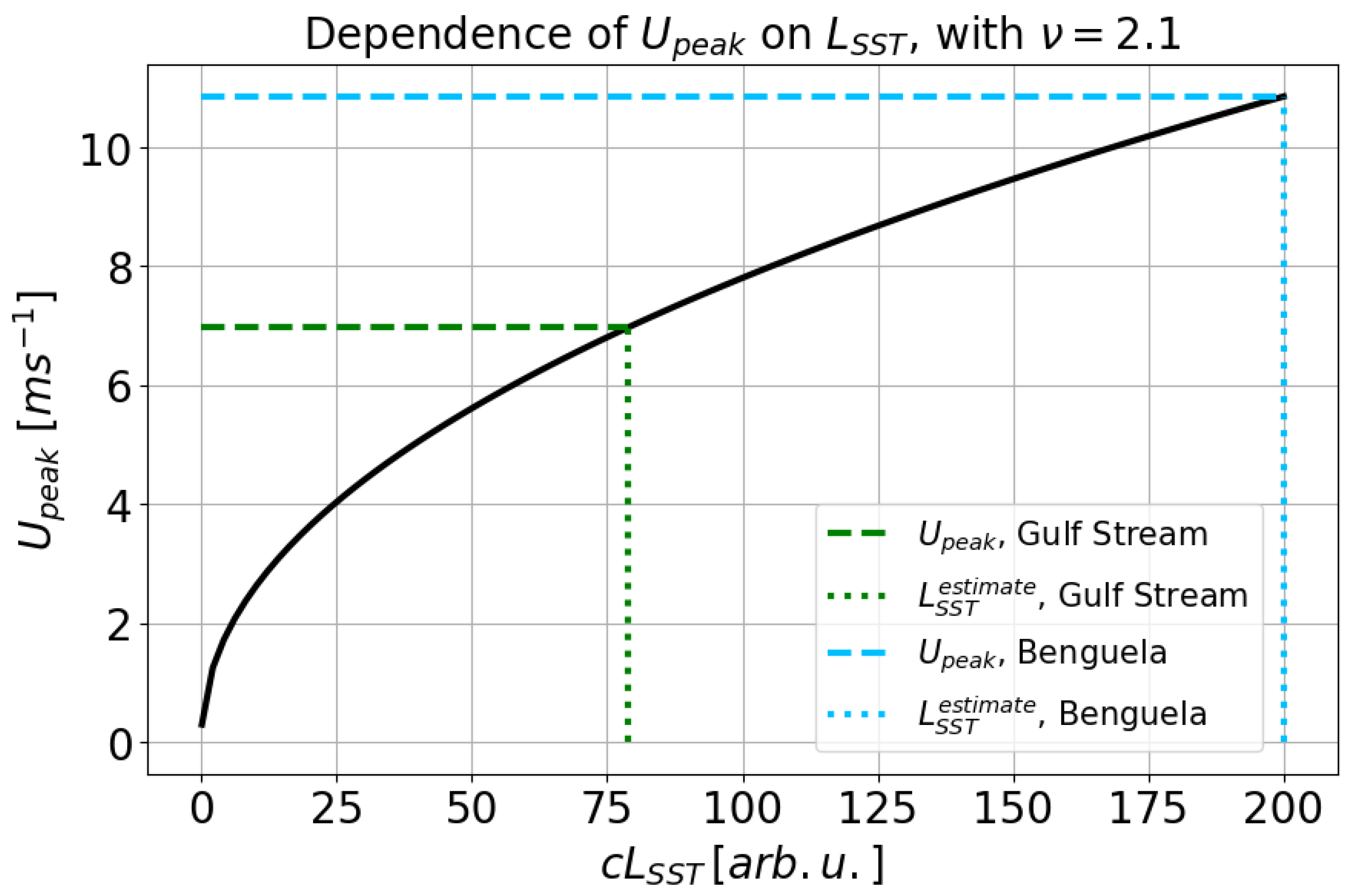
Our physical understanding suggests that the first baroclinic Rossby radius of deformation can represent the characteristic length scale of the SST forcing features. We can exploit the empirical model introduced above to argue that the data agree with this. In fact, we can compute the analytical peak velocity by setting the first derivative of equal to zero, namely
which gives an implicit definition of as a function of as
By selecting the value of , we can estimate the peak velocities from the MetOp data in the Gulf Stream and the Benguela regions in unstable conditions, which correspond to 7 m/s and 12 m/s, respectively. Then, with the implicit function, we estimate the corresponding values of and compute their ratio, as the constant c contains many free parameters that we are not able to constrain at this stage. Supposing, then, that c is the same in both regions, the ratio can be computed and it is verified to be in agreement with the ratio of the first baroclinic Rossby radius of deformation for the two regions [59].
Figure 7.
Dependence of the peak wind speed as a function of the SST characteristic length scale multiplied by the factor c, obtained from Equation 16 for . Horizontal dashed lines represent the observed values for the Gulf Stream (green) and the Benguela Current (light blue), and vertical dotted ones the corresponding values.
4. Discussion and conclusions
Mesoscale air-sea interactions have an important impact on surface fluxes, cloudiness, rainfall, and MABL dynamics, with potential inverse-cascade effects at larger scales[3,7,8,9,10,11,12,13,14]. Previous works have highlighted the dependency of air-sea coupling on environmental conditions such as surface wind, atmospheric stability and Rossby number[37,39]. In particular, Desbiolles et al. (2023) found a relevant role of large-scale surface wind (U) and air-sea temperature difference () in modulating the coupling intensity between sea surface temperature (SST) and surface wind using ERA5 reanalysis data [38]. Studies comparing numerical simulations indicate that the model representation of these air–sea interactions is influenced by the design of atmosphere-ocean coupling, the spatial and temporal resolutions, and the choice of the MABL scheme [23,30,31], underscoring the need for analysis on observational data to properly understand the physical processes.
In this work, we analyse the dependence of the DMM coupling on U and using MetOp A satellite data of ASCAT surface wind and AVHRR SST. We highlight relevant differences compared to reanalysis data in Desbiolles et al. (2023): due to its coarser resolution, ERA5 presents a larger SST characteristic length scale () than the satellite observations. This corresponds to larger advective timescales , which determines the shape of the coupling coefficient as a function of U, with the peak occurring at a larger velocity. With respect to , ERA5 does not properly represent the coupling in the stable regime for reasons possibly linked to the difficulties in the numerical representation of turbulence in these conditions. It is known, in fact, that ERA5 is characterized by important biases in representing stable boundary layers, with a tendency to overestimate the MABL height h [44,56].
We investigated if these discrepancies could be due to the different standard deviation of the Gaussian filter () used to separate large-scale wind from surface wind anomalies in observations ( km, following Meroni et al. (2023) [35]) and reanalysis ( km, following Desbiolles et al. (2023) [38]). Very little variability in the coupling coefficient behaviour was observed when testing for different in both products. In fact, according to Mishra et al. (2025) and Chelton and Xie (2010) [2,31], the coupling coefficients are expected to change significantly for scales larger than 500 km, which were removed in all the tests performed. Moreover, spatial derivatives applied to wind-field anomalies in the coupling coefficient computation act as a high-pass filter, reducing the sensitivity of the analysis to the Gaussian filter size. For these reasons, although the filters used in the two analyses differ by roughly one order of magnitude, we consider both coupling coefficient estimates to be representative of mesoscale dynamics, and therefore their behaviour with respect to the environmental conditions to be comparable.
Regional analyses show a widespread variability in the coupling behaviour which is not captured by the characterisation of the atmospheric conditions through U and solely. The nature and localisation of these discrepancies seem to suggest the relevance of h and in this sense. In particular, and h play a role in the balance between advective and response timescales, since , which determines the decoupling between the SST forcing and the wind response. At fixed latitudes (i.e. fixed ), the intensity of the coupling is found to be dependent on h, as a shallow boundary layer presents a smaller mass of air to mix compared to a deep one, and therefore shows a stronger sensitivity to the SST forcing. Unexpected results observed for stable regimes suggest that a characterisation of the MABL vertical profiles, together with a more complete description of including the momentum eddy diffusion coefficient, could provide additional insights to explain uncaptured behaviours.
Starting from the observations, we propose an empirical model (Equation 13) to interpret the coupling variability as a function of U, which advances our understanding of the relevant features, such as and h, determining the coupling intensity. The model parameters are found through a fit of the aggregated observations over the western boundary currents (WBCs) only, as tropical regions do not provide a range of U large enough to fit. As suggested by Kitaigorodskii et al., we consider stable and unstable conditions separately, as we expect different scaling of h with U in the two regimes [61]. The fit yields for unstable conditions and for stable ones. For comparison, several scalings for and h are found in the literature:
All in all, the literature indicate , with , which is well-matched by our findings.
In conclusion, observations have confirmed the physical interpretation of the control of large-scale wind (U) and atmospheric stability () on the mesoscale SST-wind coupling emerging from global ERA5 data. Nevertheless, the discrepancies between reanalysis and observations in stable conditions at the global scale, together with the widespread nonlinearities revealed in regional analyses, indicate that ERA5 may lack the ability to adequately represent these interactions in specific atmospheric conditions and regional contexts. These findings highlight the need for high-resolution observational studies to investigate mesoscale and submesoscale air-sea interactions and to support and corroborate results from numerical simulations.
The absence of high-resolution satellite measurements of MABL properties such as stability, surface fluxes, and cloudiness constitutes a critical limitation. Nevertheless, recent studies have demonstrated important progress: surface fluxes have been inferred from SAR (Synthetic Aperture Radar) roughness data, enabling estimates of atmospheric stability at resolutions of O(10 km) [63], and SAR observations are being employed to retrieve surface winds at scales of O(1 km), albeit with certain limitations [64,65]. To overcome this gap, the European Space Agency (ESA) will launch the Earth Explorer 10 mission Harmony in 2029, designed to provide SAR imagery obtained from a novel dual line-of-sight geometry together with O(1 km) SST observations. This mission will provide the necessary observation to perform a systematic assessment of air–sea interactions at the meso- and submesoscale based on instantaneous observations, with the potential to advance the understanding of their link with low-level clouds, thereby significantly improving the representation of the Earth’s radiative balance.
Author Contributions
Conceptualization, D.L.F, M.A.N. and P.C.; methodology, D.L.F, M.A.N. and P.C.; software, D.L.F.; validation, D.L.F; formal analysis, D.L.F.; investigation, D.L.F.; resources, P.C.; data curation, D.L.F.; writing—original draft preparation, D.L.F.; writing—review and editing, D.L.F., M.A.N. and P.C.; visualization, D.L.F.; supervision, P.C. and M.A.N.; project administration, P.C.; funding acquisition, P.C. All authors have read and agreed to the published version of the manuscript.
Funding
This work is an outcome of the Italian Research Ministry Project “Dipartimenti di Eccellenza 2023–2027".
Data Availability Statement
SST data from MetOp A AVHRR instrument1 and ERA5 reanalysis data 2 have been downloaded from Copernicus Climate Change Service (C3S) Climate Data Store (CDS) portal (last visit: Sept 20th, 2025). Surface wind data from MetOp A ASCAT instrument 3 come from NASA EarthDATA portal (last visit: Sept 20th, 2025). Python scripts for pre-processing and analysis are available on GitHub4.
Acknowledgments
We would like to thank Alessandro Storer, Matteo Borgnino, Fabien Desbiolles, Lionel Renault, Paco Lopez Dekker, Louise Nuijens, Owen O’Driscoll, Jacotte Monroe, Edoardo Foschi, Pouriya Alinaghi, Sara Porchetta, Xuanyu Chen, Chris Chapman and Geet George for the valuable discussions that contributed to this work.
Conflicts of Interest
The authors declare no conflicts of interest. The funders had no role in the design of the study; in the collection, analyses, or interpretation of data; in the writing of the manuscript; or in the decision to publish the results.
Appendix A. Empirical model fitting
We adopt a 2-step fitting procedure for the empirical model parameter estimation, whose results are plotted in Figure 6. First, we expect to scale with U for , so we fit coupling coefficient estimates in this interval (Figure 6, in blue) with a function in the form
obtaining the estimates of , and reported in the legend. From a physical point of view, is the contribution of fine-scale phenomena other than DMM, such that for , and for , being the threshold wind speed at which DMM becomes the dominant mesoscale process in the along-U direction.
References
- Liu, W.T.; Zhang, A.; Bishop, J.K. Evaporation and solar irradiance as regulators of sea surface temperature in annual and interannual changes. Journal of Geophysical Research: Oceans 1994, 99, 12623–12637. [Google Scholar] [CrossRef]
- Chelton, D.B.; Xie, S.P. Coupled ocean-atmosphere interaction at oceanic mesoscales. Oceanography 2010, 23, 54–69. [Google Scholar] [CrossRef]
- Small, R.J.; deSzoeke, S.P.; Xie, S.P.; O’Neill, L.; Seo, H.; Song, Q.; Cornillon, P.; Spall, M.; Minobe, S. Air–sea interaction over ocean fronts and eddies. Dynamics of Atmospheres and Oceans 2008, 45, 274–319. [Google Scholar] [CrossRef]
- Seo, H.; O’Neill, L.W.; Bourassa, M.A.; Czaja, A.; Drushka, K.; Edson, J.B.; Fox-Kemper, B.; Frenger, I.; Gille, S.T.; Kirtman, B.P.; et al. Ocean Mesoscale and Frontal-Scale Ocean-Atmosphere Interactions and Influence on Large-Scale Climate: A Review. Journal of Climate 2023, 36. [Google Scholar] [CrossRef]
- Rai, S.; Hecht, M.; Maltrud, M.; Aluie, H. Scale of oceanic eddy killing by wind from global satellite observations. Science Advances 2021, 7. [Google Scholar] [CrossRef] [PubMed]
- Gentemann, C.L.; Clayson, C.A.; Brown, S.; Lee, T.; Parfitt, R.; Farrar, J.T.; Bourassa, M.; Minnett, P.J.; Seo, H.; Gille, S.T.; et al. FluxSat: Measuring the Ocean–Atmosphere Turbulent Exchange of Heat and Moisture from Space. Remote Sensing 2020, Vol. 12, Page 1796 2020, 12, 1796. [Google Scholar] [CrossRef]
- Chelton, D.B.; Schlax, M.G.; Freilich, M.H.; Milliff, R.F. Satellite Measurements Reveal Persistent Small-Scale Features in Ocean Winds. Science 2004, 303. [Google Scholar] [CrossRef]
- Minobe, S.; Kuwano-Yoshida, A.; Komori, N.; Xie, S.P.; Small, R.J. Influence of the Gulf Stream on the troposphere. Nature 2008, 452, 206–209. [Google Scholar] [CrossRef]
- Minobe, S.; Miyashita, M.; Kuwano-Yoshida, A.; Tokinaga, H.; Xie, S.P. Atmospheric response to the Gulf Stream: Seasonal variations. Journal of Climate 2010, 23. [Google Scholar] [CrossRef]
- Small, R.J.; Rousseau, V.; Parfitt, R.; Laurindo, L.; O’Neill, L.; Masunaga, R.; Schneider, N.; Chang, P. Near-Surface Wind Convergence over the Gulf Stream—The Role of SST Revisited. Journal of Climate 2023, 36, 5527–5548. [Google Scholar] [CrossRef]
- Ma, X.; Jing, Z.; Chang, P.; Liu, X.; Montuoro, R.; Small, R.J.; Bryan, F.O.; Greatbatch, R.J.; Brandt, P.; Wu, D.; et al. Western boundary currents regulated by interaction between ocean eddies and the atmosphere. Nature 2016, 535, 533–537. [Google Scholar] [CrossRef] [PubMed]
- Frenger, I.; Gruber, N.; Knutti, R.; Münnich, M. Imprint of Southern Ocean eddies on winds, clouds and rainfall. Nature Geoscience 2013, 6. [Google Scholar] [CrossRef]
- Parfitt, R.; Czaja, A.; Minobe, S.; Kuwano-Yoshida, A. The atmospheric frontal response to SST perturbations in the Gulf Stream region. Geophysical Research Letters 2016, 43, 2299–2306. [Google Scholar] [CrossRef]
- Hirata, H.; Kawamura, R.; Nonaka, M.; Tsuboki, K. Significant Impact of Heat Supply From the Gulf Stream on a “Superbomb” Cyclone in January 2018. Geophysical Research Letters 2019, 46, 7718–7725. [Google Scholar] [CrossRef]
- Gaube, P.; Chickadel, C.C.; Branch, R.; Jessup, A. Satellite Observations of SST-Induced Wind Speed Perturbation at the Oceanic Submesoscale. Geophysical Research Letters 2019, 46, 2690–2695. [Google Scholar] [CrossRef]
- Strobach, E.; Klein, P.; Molod, A.; Fahad, A.A.; Trayanov, A.; Menemenlis, D.; Torres, H. Local Air-Sea Interactions at Ocean Mesoscale and Submesoscale in a Western Boundary Current. Geophysical Research Letters 2022, 49. [Google Scholar] [CrossRef]
- Renault, L.; Contreras, M.; Marchesiello, P.; Conejero, C.; Uchoa, I.; Wenegrat, J. Unraveling the Impacts of Submesoscale Thermal and Current Feedbacks on the Low-Level Winds and Oceanic Submesoscale Currents. Journal of Physical Oceanography 2024, 54, 2463–2486. [Google Scholar] [CrossRef]
- Bai, Y.; Thompson, A.F.; Bôas, A.B.V.; Klein, P.; Torres, H.S.; Menemenlis, D. Sub-Mesoscale Wind-Front Interactions: The Combined Impact of Thermal and Current Feedback. Geophysical Research Letters 2023, 50. [Google Scholar] [CrossRef]
- Conejero, C.; Renault, L.; Desbiolles, F.; McWilliams, J.C.; Giordani, H. Near-Surface Atmospheric Response to Meso- and Submesoscale Current and Thermal Feedbacks. Journal of Physical Oceanography 2024, 54, 823–848. [Google Scholar] [CrossRef]
- Nuijens, L.; Wenegrat, J.; Dekker, P.L.; Pasquero, C.; L.W., O.; Ardhuin, F.; Ayet, A.; Bechtold, P.; Bruch, W.; Laurindo, L.; et al. The air-sea interaction (ASI) submesoscale: Physics and impact. [CrossRef]
- Renault, L.; Molemaker, M.J.; Mcwilliams, J.C.; Shchepetkin, A.F.; Lemarié, F.; Chelton, D.; Illig, S.; Hall, A. Modulation of Wind Work by Oceanic Current Interaction with the Atmosphere. Journal of Physical Oceanography 2016, 46, 1685–1704. [Google Scholar] [CrossRef]
- Takatama, K.; Schneider, N. The Role of Back Pressure in the Atmospheric Response to Surface Stress Induced by the Kuroshio. Journal of the Atmospheric Sciences 2017, 74, 597–615. [Google Scholar] [CrossRef]
- Renault, L.; Masson, S.; Oerder, V.; Jullien, S.; Colas, F. Disentangling the Mesoscale Ocean-Atmosphere Interactions. Journal of Geophysical Research: Oceans 2019, 124, 2164–2178. [Google Scholar] [CrossRef]
- Wallace, J.M.; Mitchell, T.P.; Deser, C. The Influence of Sea-Surface Temperature on Surface Wind in the Eastern Equatorial Pacific: Seasonal and Interannual Variability. Journal of Climate 1989, 2. [Google Scholar] [CrossRef]
- Hayes, S.P.; McPhaden, M.J.; Wallace, J.M. The Influence of Sea-Surface Temperature on Surface Wind in the Eastern Equatorial Pacific: Weekly to Monthly Variability. Journal of Climate 1989, 2, 1500–1506. [Google Scholar] [CrossRef]
- Lindzen, R.S.; Nigam, S. On the Role of Sea Surface Temperature Gradients in Forcing Low-Level Winds and Convergence in the Tropics. Journal of the Atmospheric Sciences 1987, 44. [Google Scholar] [CrossRef]
- Desbiolles, F.; Alberti, M.; Hamouda, M.E.; Meroni, A.N.; Pasquero, C. Links Between Sea Surface Temperature Structures, Clouds and Rainfall: Study Case of the Mediterranean Sea. Geophysical Research Letters 2021, 48. [Google Scholar] [CrossRef]
- Chelton, D.B.; Esbensen, S.K.; Schlax, M.G.; Thum, N.; Freilich, M.H.; Wentz, F.J.; Gentemann, C.L.; Mcphaden, M.J.; Schopf, P.S. Observations of Coupling between Surface Wind Stress and Sea Surface Temperature in the Eastern Tropical Pacific. Technical report, 2001. [CrossRef]
- O’Neill, L.W.; Chelton, D.B.; Esbensen, S.K. Observations of SST-Induced Perturbations of the Wind Stress Field over the Southern Ocean on Seasonal Timescales. Journal of Climate 2003, 16, 2340–2354. [Google Scholar] [CrossRef]
- Bryan, F.O.; Tomas, R.; Dennis, J.M.; Chelton, D.B.; Loeb, N.G.; Mcclean, J.L. Frontal Scale Air–Sea Interaction in High-Resolution Coupled Climate Models. Journal of Climate 2010, 23, 6277–6291. [Google Scholar] [CrossRef]
- Mishra, A.K.; Meroni, A.N.; Strobach, E.; Jangir, B. Effects of the Grid Spacing and Background Wind on the Daily Air-Sea Coupling Over the Mediterranean Sea in HighResMIP. Journal of Geophysical Research: Atmospheres 2025, 130, e2024JD041686. [Google Scholar] [CrossRef]
- Oerder, V.; Colas, F.; Echevin, V.; Masson, S.; Hourdin, C.; Jullien, S.; Madec, G.; Lemarié, F. Mesoscale SST–wind stress coupling in the Peru–Chile current system: Which mechanisms drive its seasonal variability? Climate Dynamics 2016, 47, 2309–2330. [Google Scholar] [CrossRef]
- Perlin, N.; Szoeke, S.P.D.; Chelton, D.B.; Samelson, R.M.; Skyllingstad, E.D.; O’neill, L.W. Modeling the Atmospheric Boundary Layer Wind Response to Mesoscale Sea Surface Temperature Perturbations. Monthly Weather Review 2014, 142, 4284–4307. [Google Scholar] [CrossRef]
- Sandu, I.; Bechtold, P.; Nuijens, L.; Beljaars, A.; Brown, A. On the causes of systematic forecast biases in near-surface wind direction over the oceans Near-surface wind direction biases 2020. [CrossRef]
- Meroni, A.N.; Desbiolles, F.; Pasquero, C. Satellite signature of the instantaneous wind response to mesoscale oceanic thermal structures. Quarterly Journal of the Royal Meteorological Society 2023. [Google Scholar] [CrossRef]
- Meroni, A.N.; Giurato, M.; Ragone, F.; Pasquero, C. Observational evidence of the preferential occurrence of wind convergence over sea surface temperature fronts in the Mediterranean. Quarterly Journal of the Royal Meteorological Society 2020, 146, 1443–1458. [Google Scholar] [CrossRef]
- Foussard, A.; Lapeyre, G.; Plougonven, R. Response of Surface Wind Divergence to Mesoscale SST Anomalies under Different Wind Conditions. Journal of the Atmospheric Sciences 2019, 76, 2065–2082. [Google Scholar] [CrossRef]
- Desbiolles, F.; Meroni, A.N.; Renault, L.; Pasquero, C. Environmental Control of Wind Response to Sea Surface Temperature Patterns in Reanalysis Dataset. Journal of Climate 2023. [Google Scholar] [CrossRef]
- Schneider, N. Scale and rossby number dependence of observed wind responses to ocean-mesoscale sea surface temperatures. Journal of the Atmospheric Sciences 2020, 77, 3171–3192. [Google Scholar] [CrossRef]
- Rivas, M.B.; Stoffelen, A. Characterizing ERA-Interim and ERA5 surface wind biases using ASCAT. Ocean Science 2019, 15, 831–852. [Google Scholar] [CrossRef]
- Vogelzang, J.; Stoffelen, A.; Verhoef, A.; Figa-Saldaña, J. On the quality of high-resolution scatterometer winds. Journal of Geophysical Research: Oceans 2011, 116, 10033. [Google Scholar] [CrossRef]
- Bolgiani, P.; Calvo-Sancho, C.; Díaz-Fernández, J.; Quitián-Hernández, L.; Sastre, M.; Santos-Muñoz, D.; Farrán, J.I.; González-Alemán, J.J.; Valero, F.; Martín, M.L. Wind kinetic energy climatology and effective resolution for the ERA5 reanalysis. Climate Dynamics 2022, 59, 737–752. [Google Scholar] [CrossRef]
- Seethala, C.; Zuidema, P.; Edson, J.; Brunke, M.; Chen, G.; Li, X.Y.; Painemal, D.; Robinson, C.; Shingler, T.; Shook, M.; et al. On Assessing ERA5 and MERRA2 Representations of Cold-Air Outbreaks Across the Gulf Stream. Geophysical Research Letters 2021, 48, e2021GL094364. [Google Scholar] [CrossRef]
- Hersbach, H.; Bell, B.; Berrisford, P.; Hirahara, S.; Horányi, A.; Muñoz-Sabater, J.; Nicolas, J.; Peubey, C.; Radu, R.; Schepers, D.; et al. The ERA5 global reanalysis. Quarterly Journal of the Royal Meteorological Society 2020, 146, 1999–2049. [Google Scholar] [CrossRef]
- Bishop, S.P.; Small, R.J.; Bryan, F.O. The Global Sink of Available Potential Energy by Mesoscale Air-Sea Interaction. Journal of Advances in Modeling Earth Systems 2020, 12, e2020MS002118. [Google Scholar] [CrossRef]
- Embury, O.; Bulgin, C.E.; Mittaz, J. ESA Sea Surface Temperature Climate Change Initiative (SST_cci): Advanced Very High Resolution Radiometer (AVHRR) Level 3 Collated (L3C) Climate Data Record, version 2. 1 2019. [Google Scholar] [CrossRef]
- Merchant, C.J.; Embury, O.; Bulgin, C.E.; Block, T.; Corlett, G.K.; Fiedler, E.; Good, S.A.; Mittaz, J.; Rayner, N.A.; Berry, D.; et al. Satellite-based time-series of sea-surface temperature since 1981 for climate applications 2019. [CrossRef]
- Verhoef, A.; Vogelzang, J.; Verspeek, J.; Stoffelen, A. Long-Term Scatterometer Wind Climate Data Records. IEEE Journal of Selected Topics in Applied Earth Observations and Remote Sensing 2017, 10, 2186–2194. [Google Scholar] [CrossRef]
- Kettle, A.J. A Diagram of Wind Speed Versus Air-sea Temperature Difference to Understand the Marine atmospheric Boundary Layer. Energy Procedia 2015, 76, 138–147. [Google Scholar] [CrossRef]
- Meroni, A.N.; Desbiolles, F.; Pasquero, C. Introducing New Metrics for the Atmospheric Pressure Adjustment to Thermal Structures at the Ocean Surface. Journal of Geophysical Research: Atmospheres 2022, 127. [Google Scholar] [CrossRef]
- Press, W.H.; Teukolsky, S.A.; Vetterling, W.T.; Flannery, B.P. Numerical recipes : the art of scientific computing; Cambridge University Press, 2007; p. 1235.
- Bane, J.M.; Osgood, K.E. Wintertime air-sea interaction processes across the Gulf Stream. Journal of Geophysical Research: Oceans 1989, 94, 10755–10772. [Google Scholar] [CrossRef]
- Stevens, B.; Bony, S.; Farrell, D.; Ament, F.; Blyth, A.; Fairall, C.; Karstensen, J.; Quinn, P.; Speich, S.; Acquistapace, C.; et al. EUREC4A. Earth System Science Data 2021, 13. [Google Scholar] [CrossRef]
- Obukhov, A.M. Turbulence in an atmosphere with a non-uniform temperature. Boundary-Layer Meteorology 1971, 2. [Google Scholar] [CrossRef]
- Zilitinkevich, S.; Baklanov, A. Calculation of the height of the stable boundary layer in practical applications. Boundary-Layer Meteorology 2002, 105, 389–409. [Google Scholar] [CrossRef]
- Davy, R.; Esau, I. Global climate models’ bias in surface temperature trends and variability. Environmental Research Letters 2014, 9, 114024. [Google Scholar] [CrossRef]
- Kalmus, P.; Ao, C.O.; Wang, K.N.; Manzi, M.P.; Teixeira, J. A high-resolution planetary boundary layer height seasonal climatology from GNSS radio occultations. Remote Sensing of Environment 2022, 276, 113037. [Google Scholar] [CrossRef]
- Fernández, P.; Speich, S.; Borgnino, M.; Meroni, A.N.; Desbiolles, F.; Pasquero, C. On the importance of the atmospheric coupling to the small-scale ocean in the modulation of latent heat flux. Frontiers in Marine Science 2023, 10, 1136558. [Google Scholar] [CrossRef]
- Chelton, D.B.; Deszoeke, R.A.; Schlax, M.G.; Naggar, K.E.; Siwertz, N. Geographical Variability of the First Baroclinic Rossby Radius of Deformation. Journal of Physical Oceanography 1998, 28, 433–460. [Google Scholar] [CrossRef]
- Arya, S.P. Parameterizing the Height of the Stable Atmospheric Boundary Layer. Journal of Applied Meteorology and Climatology 1981, 20, 1192–1202. [Google Scholar] [CrossRef]
- Kitaigorodskii, S.A.; Joffre, S.M. In search of a simple scaling for the height of the stratified atmospheric boundary layer. Tellus, Series A 1988, 40 A, 419–433. [CrossRef]
- Nieuwstadt, F.T.M. The Turbulent Structure of the Stable, Nocturnal Boundary Layer. Journal of Atmospheric Sciences 1984, 41, 2202–2216. [Google Scholar] [CrossRef]
- O’Driscoll, O.; Mouche, A.; Chapron, B.; Kleinherenbrink, M.; López-Dekker, P. Obukhov Length Estimation From Spaceborne Radars. Geophysical Research Letters 2023, 50. [Google Scholar] [CrossRef]
- Bourassa, M.A.; Meissner, T.; Cerovecki, I.; Chang, P.S.; Dong, X.; Chiara, G.D.; Donlon, C.; Dukhovskoy, D.S.; Elya, J.; Fore, A.; et al. Remotely Sensed Winds and Wind Stresses for Marine Forecasting and Ocean Modeling. Frontiers in Marine Science 2019, 6. [Google Scholar] [CrossRef]
- Zanchetta, A.; Zecchetto, S. Wind direction retrieval from Sentinel-1 SAR images using ResNet. Remote Sensing of Environment 2021, 253. [Google Scholar] [CrossRef]
| 1 | |
| 2 | |
| 3 | |
| 4 |
Figure 1.
Domains for regional analysis and SST field on the 1st of September 2020 from ERA5 (in the background). Yellow lines highlight the boundaries of the global domain (between -60° and 60° latitude).
Figure 1.
Domains for regional analysis and SST field on the 1st of September 2020 from ERA5 (in the background). Yellow lines highlight the boundaries of the global domain (between -60° and 60° latitude).
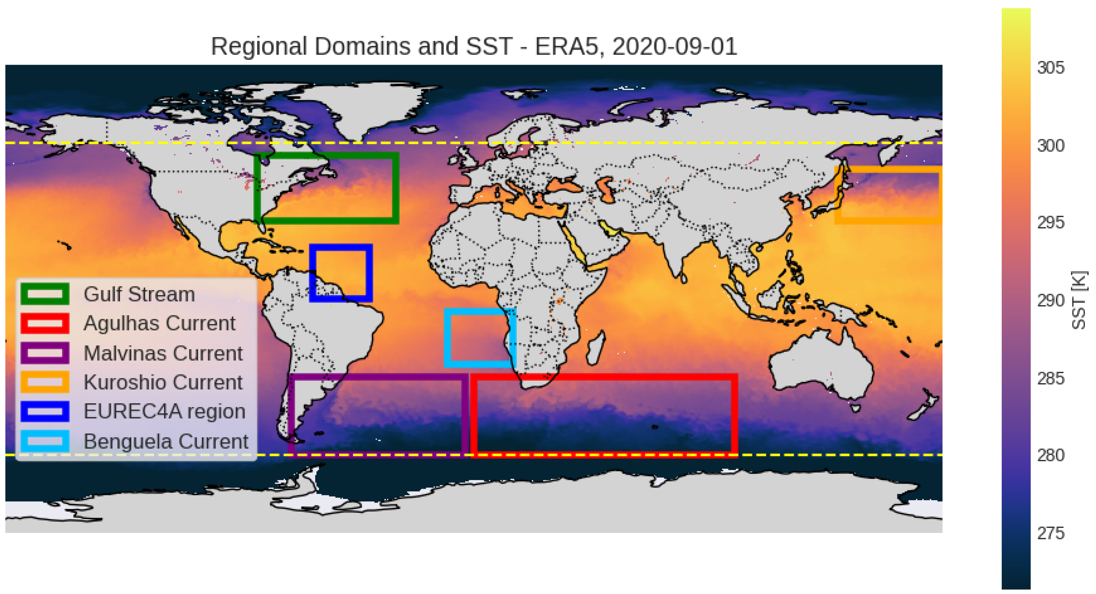
Figure 2.
DMM coupling coefficient as a function of large-scale surface wind speed U (a) and air-sea temperature difference (b) from global MetOp observations (full line) and ERA5 data (dash line).
Figure 2.
DMM coupling coefficient as a function of large-scale surface wind speed U (a) and air-sea temperature difference (b) from global MetOp observations (full line) and ERA5 data (dash line).
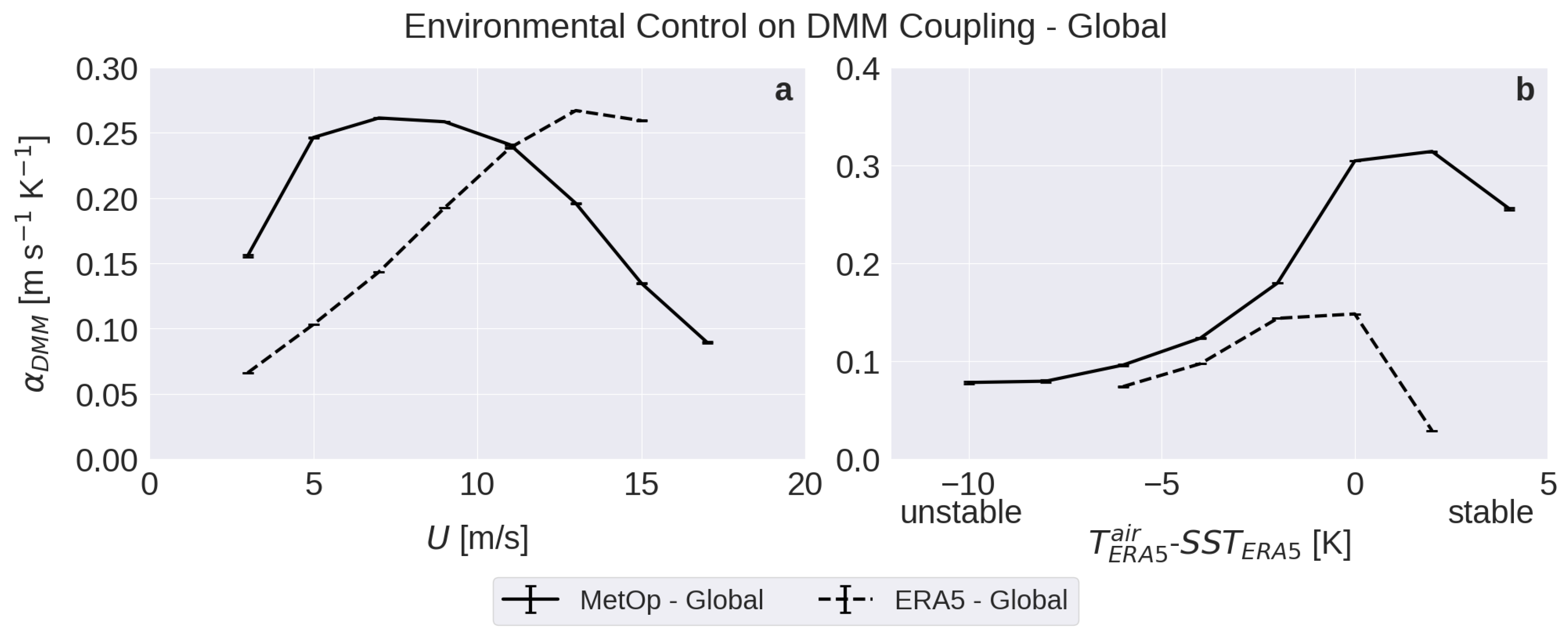
Figure 3.
Combined dependence of on U and (a) from global MetOp data with the corresponding standard deviation (b).
Figure 3.
Combined dependence of on U and (a) from global MetOp data with the corresponding standard deviation (b).
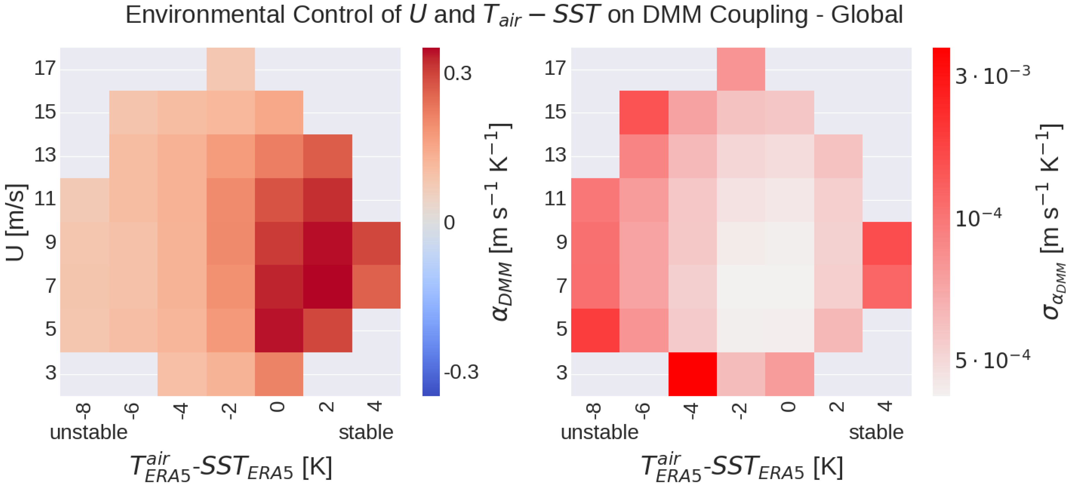
Figure 4.
DMM coupling coefficient as a function of large-scale surface wind speed U (a,c) and air-sea temperature difference (b,d) from regional observations (a,b) and reanalysis data (c,d).
Figure 4.
DMM coupling coefficient as a function of large-scale surface wind speed U (a,c) and air-sea temperature difference (b,d) from regional observations (a,b) and reanalysis data (c,d).
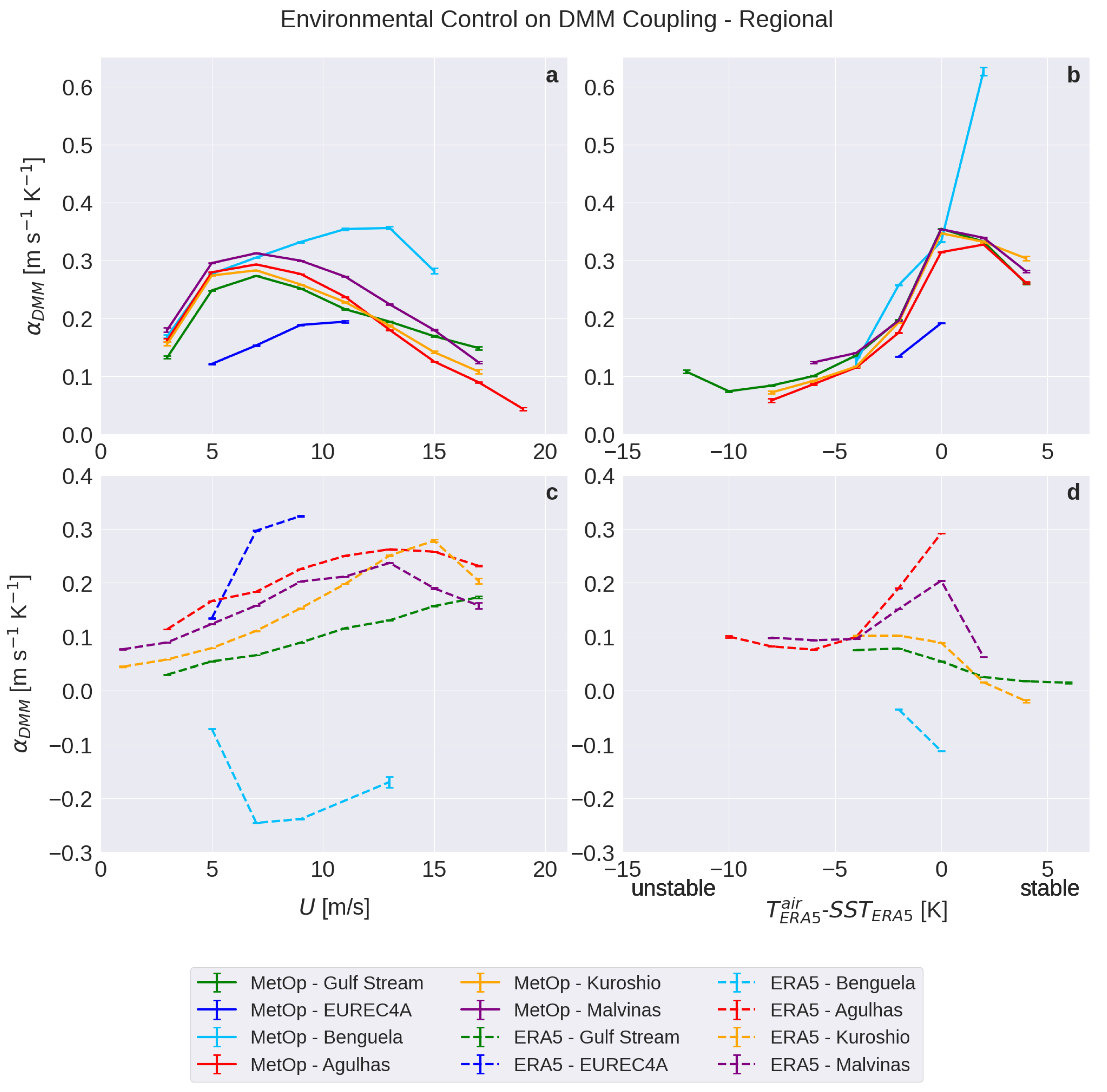
Figure 6.
Coupling coefficients as a function of U for all WBCs in stable (a) and unstable (b) conditions. Blue points denote the data used to perform the linear fit in Equation A1 for low-U. Red points are employed to fit the function for high U in Equation A2, estimating and . Dashed lines show the final curves of the fit, with the relevant parameters indicated in the legend.
Disclaimer/Publisher’s Note: The statements, opinions and data contained in all publications are solely those of the individual author(s) and contributor(s) and not of MDPI and/or the editor(s). MDPI and/or the editor(s) disclaim responsibility for any injury to people or property resulting from any ideas, methods, instructions or products referred to in the content. |
© 2025 by the authors. Licensee MDPI, Basel, Switzerland. This article is an open access article distributed under the terms and conditions of the Creative Commons Attribution (CC BY) license (http://creativecommons.org/licenses/by/4.0/).
Copyright: This open access article is published under a Creative Commons CC BY 4.0 license, which permit the free download, distribution, and reuse, provided that the author and preprint are cited in any reuse.


