Submitted:
21 October 2024
Posted:
22 October 2024
You are already at the latest version
Abstract
This paper presents a comprehensive approach to enhancing submersible safety through mathematical modeling and decision-making frameworks. We develop models for submersible location prediction, emergency preparedness, and scenario extrapolation, including a Seawater Density Model, Submersible Mechanical Model, Bayesian Searching Model, and Extended Kalman Filter. Sensitivity analysis confirms the robustness of these models under varying conditions, making them adaptable for different marine environments.In the first section, we focus on accurately locating a submersible after communication loss. The Seawater Density Model employs a hyperbolic tangent function to model depth-dependent density in the Ionian Sea, while the Submersible Mechanical Model simulates underwater dynamics using the 4th order Runge-Kutta method. Uncertainties are addressed using an Extended Kalman Filter, enhancing accuracy, as shown by trajectory and Mean Squared Error (MSE) comparisons.In the second section, we develop a Bayesian Searching Model to efficiently locate a missing submersible. This model iteratively updates location probabilities using a bimodal Gaussian distribution. The search zone is discretized into grids, and simulations demonstrate the model's ability to effectively narrow down the search area and improve detection success.In the third section, we adapt the models to different environments, such as the Caribbean Sea. A warning and obstacle avoidance system is introduced to manage multiple submersibles in close proximity, dynamically adjusting their paths to avoid collisions.Reliability analysis demonstrates the robustness of the models against changes in density and sudden environmental shifts, showing minimal deviation from neutral buoyancy. These results confirm the reliability and adaptability of the models for enhancing submersible safety across various marine settings.
Keywords:
Bayesian Searching Model
; Bimodal Gaussian Distribution
; Buoyancy
; Collision Avoidance
; Discretization
; Equations of Mathematical Physics
; Ionian Ocean
; Kalman Filter
; Runge-Kutta Method
; Searching and Rescue
; Seawater Density
; Submersible
1. Introduction
Submersibles offer unique opportunities for underwater exploration, but their safe operation faces challenges such as loss of communication, mechanical failures, and dynamic marine environments. Accurate prediction of submersible locations and effective emergency procedures are crucial for ensuring the safety of both passengers and crew.
This paper aims to:
- Develop a Seawater Density Model to represent depth-dependent density variations.
- Construct a Submersible Mechanical Model for trajectory prediction.
- Propose a Bayesian Searching Model and Extended Kalman Filter for locating missing submersibles.
- Perform sensitivity analysis and extrapolate models to other environments.
2. Locate
To precisely locate the submersible, we developed two key models: the Seawater Density Model and the Submersible Mechanical Model. These models allow us to accurately determine the submersible’s position after losing communication by analyzing both the surrounding environment and the dynamics of the submersible itself.
2.1. Seawater Density Model
The first step in predicting the movement of the submersible is to analyze the environment, specifically the seawater density, which determines both the buoyancy and neutral buoyancy depth of the submersible. This is essential for understanding the submersible’s equilibrium behavior.
2.1.1. Seawater Density Stratification
The density of seawater varies due to thermohaline stratification, which refers to the changes in temperature and salinity at different depths [3]. Surface waters are generally warmer and less saline, leading to lower density, while deep waters are colder, saltier, and therefore denser.
Based on literature [2] and our assumptions, we model seawater density as a hyperbolic tangent function of depth, . The density generally increases with depth due to higher pressure and changes in temperature and salinity, resulting in a nonlinear relationship.
Here, represents the sea-level water density, represents the density increment for each layer, and controls the steepness of the density gradient.
Figure 1.
Fitted density stratification of seawater.
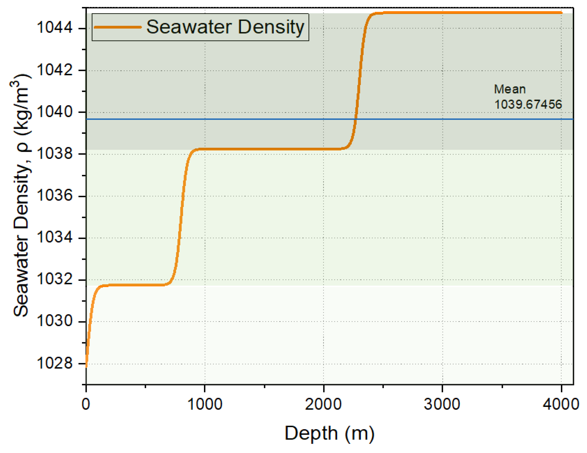
Using this model, we stratify seawater into three layers with distinct pycnoclines. The mean density of seawater in our study area is found to be 1039.67 kg/m³.
2.2. Submersible Mechanical Model
After analyzing the seawater density, we then model the submersible itself. This involves both static and dynamic analysis to understand how the submersible moves in response to various forces.
2.2.1. Static Buoyancy Analysis
We first analyze the equilibrium state of the submersible. Let the submersible’s initial position and velocity at the time of losing communication be and , respectively. We assume the mass of the submersible is constant (m) and that the propulsion force (F) has an angle with respect to the x-y plane. The static buoyancy equation is given by:
Here, is the density of the submersible, and is the density of the seawater. Solving this equation provides the neutral buoyancy depth .
2.2.2. Dynamic Analysis
We then perform a dynamic analysis of the submersible, considering its movement and environmental factors. Figure 2 illustrates the free body diagram and velocity decomposition.
The submersible is subject to several forces, including propulsion (), gravity (), buoyancy (), and fluid resistance ():
We decompose the velocity into components, where is the angle between the velocity projection on the x-y plane and the x-axis, and is the angle between the velocity and the x-y plane. and represent the angles of the propulsion force with respect to the x-y plane and the x-axis.
The system of differential equations representing the submersible’s dynamics is given by:

Table 1.
Dynamic parameters for different submersibles.
| Parameter | Submersible 1 | Submersible 2 |
| Velocity (m/s) | 15 | 30 |
| Propulsion force (N) | 28 | 34 |
| Mass m (kg) | 1000 | 1000 |
| Drag coefficient | 0.5 | 0.5 |
| Reference area A () | 0.6 | 0.6 |
| () | 1022.75 | 1030.75 |
2.2.3. Boundary Conditions: Seabed Depth
The submersible’s motion is constrained by the seabed, which limits the depth the submersible can reach. Figure 3 shows the seabed depth data for the Ionian Sea [1,5].
We solved the system of differential equations using the 4th order Runge-Kutta method to accurately predict the trajectory of the submersible after losing communication. Figure 4 and Figure 5 depict two scenarios: one where the submersible hits the seabed and one where it maintains neutral buoyancy.
2.3. Uncertainties in the Model
2.3.1. Uncertainty in Mechanical Default
It is challenging to determine whether mechanical failure occurs before or after a communication loss. A monitoring system for key components can help detect failures early and trigger alarms or automated measures.
2.3.2. Noise Uncertainties and Solutions
Noise from fluid dynamics, such as ocean currents, affects the submersible’s trajectory. To improve accuracy, GPS and IMU sensors are used to provide position and velocity data, respectively. These sensors, however, introduce noise. To reduce uncertainty, we apply the Extended Kalman Filter (EKF), which is suitable for the non-linear nature of submersible motion.
The EKF prediction and update steps are [4]:
where is the Kalman gain and is the measurement innovation.
The state transition equations for submersible motion are:
2.3.3. Enhancement Model: BIKF and DKF Gaussian Noise Mixture Model
To simulate unpredictable ocean currents, we use a Gaussian Mixture Model (GMM) for non-Gaussian noise, combining small- and large-variance Gaussian noise. The Background Impulse Kalman Filter (BIKF) handles non-Gaussian noise more effectively [4]. We also apply a Distributed Kalman Filter (DKF) for data fusion [6].
3. Searching
After locating the location of the submersible, we need create a model utilizing data from previous models used in location task to suggest starting points and searching trajectories for the equipment, aiming to reduce the time needed to locate a missing submersible. We need to determine the likelihood of locating the submersible based on time and the accumulated search results.
Here, we propose a Bayesian Searching Model to solve the problem.
3.1. Bayesian Searching Model
We can have a prior probability about the submersible’s location, which can be obtained from the positioning in the first section. However, each time the rescue boat conducts a search, it brings new information about the location of the submersible. To fully utilize this information, we employ a Bayesian search model. We use the results from each search as the prior probability distribution for our next search[?]. This iterative process is aimed at minimizing the search time as much as possible.
3.1.1. Bimodal Gaussian Distribution Function
Due to the model uncertainties mentioned in the first section, we cannot determine whether the mechanical defects will happen after losing communication. So we need to consider possibilities in both situations into consideration, mechanical defects happens and no mechanical defects after signal lost. We use bimodal Gaussian Distribution to incorporate the these two situations, resembling the prior probability density of searching.
Suppose the last signal before losing communication transmit the state of submersible is . The state include the position and velocity in different directions.
From the previous analysis, the submarine will quickly enter a static state in the z-direction. Consider the influence of ocean currents and noise. we consider two situations where the submersible continues to sail and mechanical failure, representing the prior probability map at the initial moment as a bimodal Gaussian distribution [8], that is
and are respectilythe possibilities of mechanical defects and the no mechanical defects. and are the influence of noise and current in two situations respectively.
Table 2.
Parameters in bimodal Gaussian distribution function.
| parameters | value | parameters | value |
| 0.7 | 0.3 | ||
| 10 | 10 | ||
| 3800 | 3800 | ||
| 2500 | 2500 |
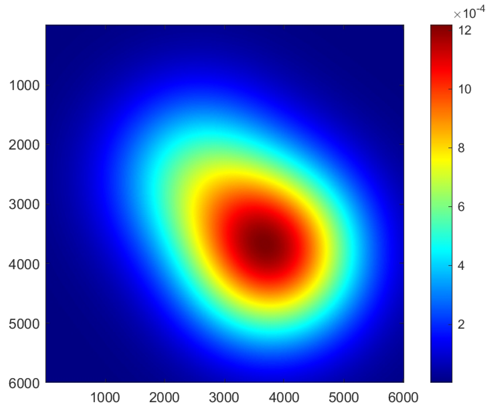
Using the bimodal Gaussian distribution function in eq (7), we select sea area of , the probability distribution graph of submersible’s location (2-dimensional) is shown below.
Figure 6.
The probability distribution graph of submersible location.
3.1.2. Discretization of Searching Possibilities (Avocado Grid Searching)
We assume the effective detection range of the rescue boat conducted is within time interval T. Assume in time interview T, the unit searching area of rescue ship is D. So we can divide the sea into grids with an area of D in our model. Which looks just like an avocado.
These grids are regarded as n non-interfering areas (). Use to represent the status in the ith area at the kth moment. The probability of each grid is the integral of the probability density in the area of the grid. , , , are the boundaries of the grid.
After calculating the probability for each grid through integration, we normalize these values for each grid point.
The probability of the sensor successfully observing the submersible at its location is denoted as q (conditional probability). p is the probability of submersible located in current observed grid. Based on Bayes’ theorem, we derived the following formula for updating the posterior probability with each combined observation: After this detection, if the submersible is not detected in this grid, the possibility of this grid under detected is renewed.
Figure 7.
Possibilities renew after current detection.
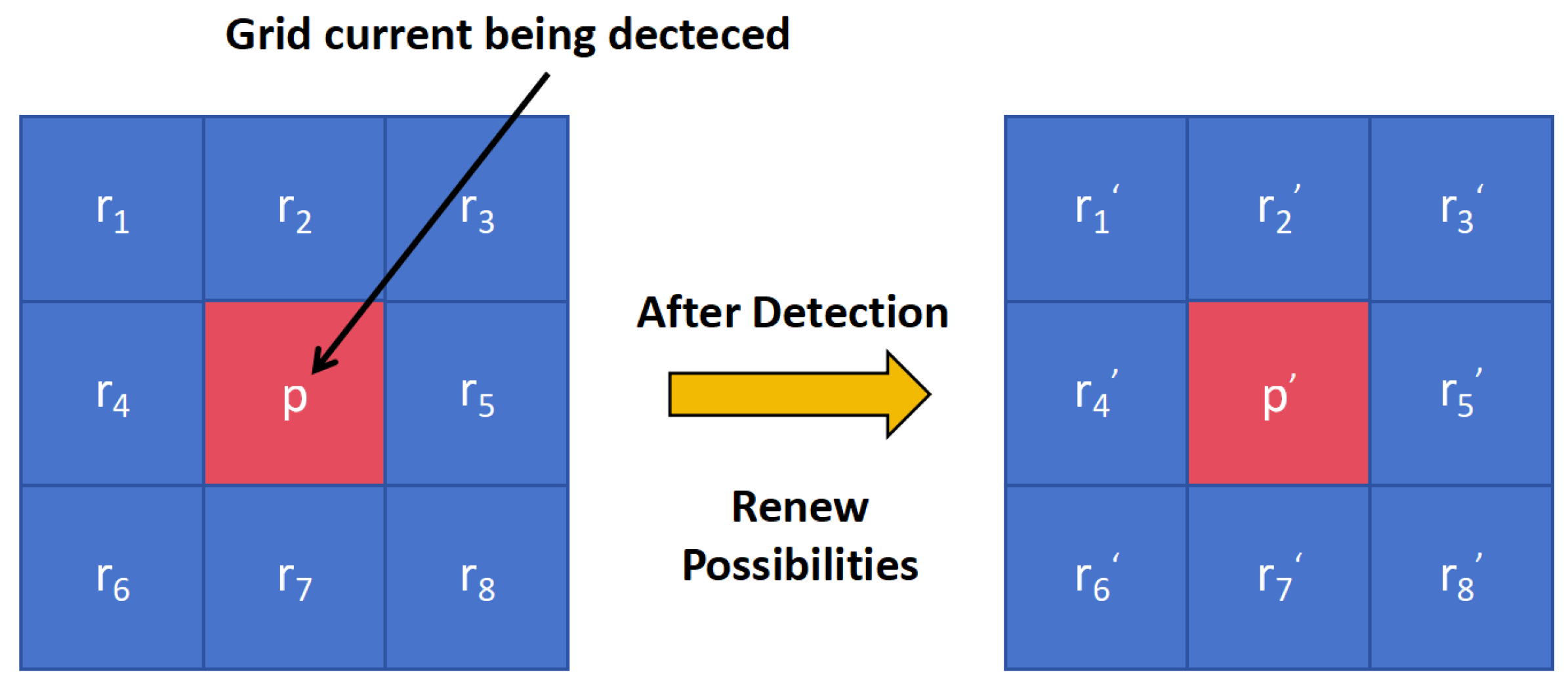
After detection, the possibility of the grid being detected is renew to
After detection, the possibility of the rest of the grids is :
Using eq (9,10), we continue to iterate the searching process, combining with the submersible mechanical model in the first section, we have the simulation of searching as Figure 8. In our case, the bimodal Gaussian distribution has a large variance. When the variance is small, a bimodal image will appear. When the variance is large, it will produce the image of an avocado that we speak of.
The previous graph shows the iteration of posterior possibilities of submersible’s location. Combining the model in locating and the searching we simulate the real search route based on the dynamic equations and Bayesian searching model of the submersible. These graphs show the MSE between different predicted trajectories and real trajectory.
Current we are simulating the overlapping process of the movement of submersible and the searching route. The red line in Figure 9(a) simulate the real movement of submersible on x-y plane. In the process of Bayesian searching iteration and the rescue boat searching, when the route of submersible is overlapped with currently searching grid, the successful searching possibilities is q, which is the largest.
3.2. The Probability of Finding the Submersible as a Function of Time and Accumulated Search Results
The probability of locating the submarine is expressed as a function of time and accumulated search results. Let be a binary variable used to determine whether the submarine is found in the ith search.
Every searching trial has two results, the submersible either being searched or not being searched. Suppose at the nth detection, the probability of the submersibles located in this searching grid is . where is derived from the prior probability before each detection.
In time , the probability of submersible being successfully searched is
Notice the ∑ summation here means or. Moreover, because of
In summary, the probability of finding the submersible as a function of time and accumulated search results can be expressed as:
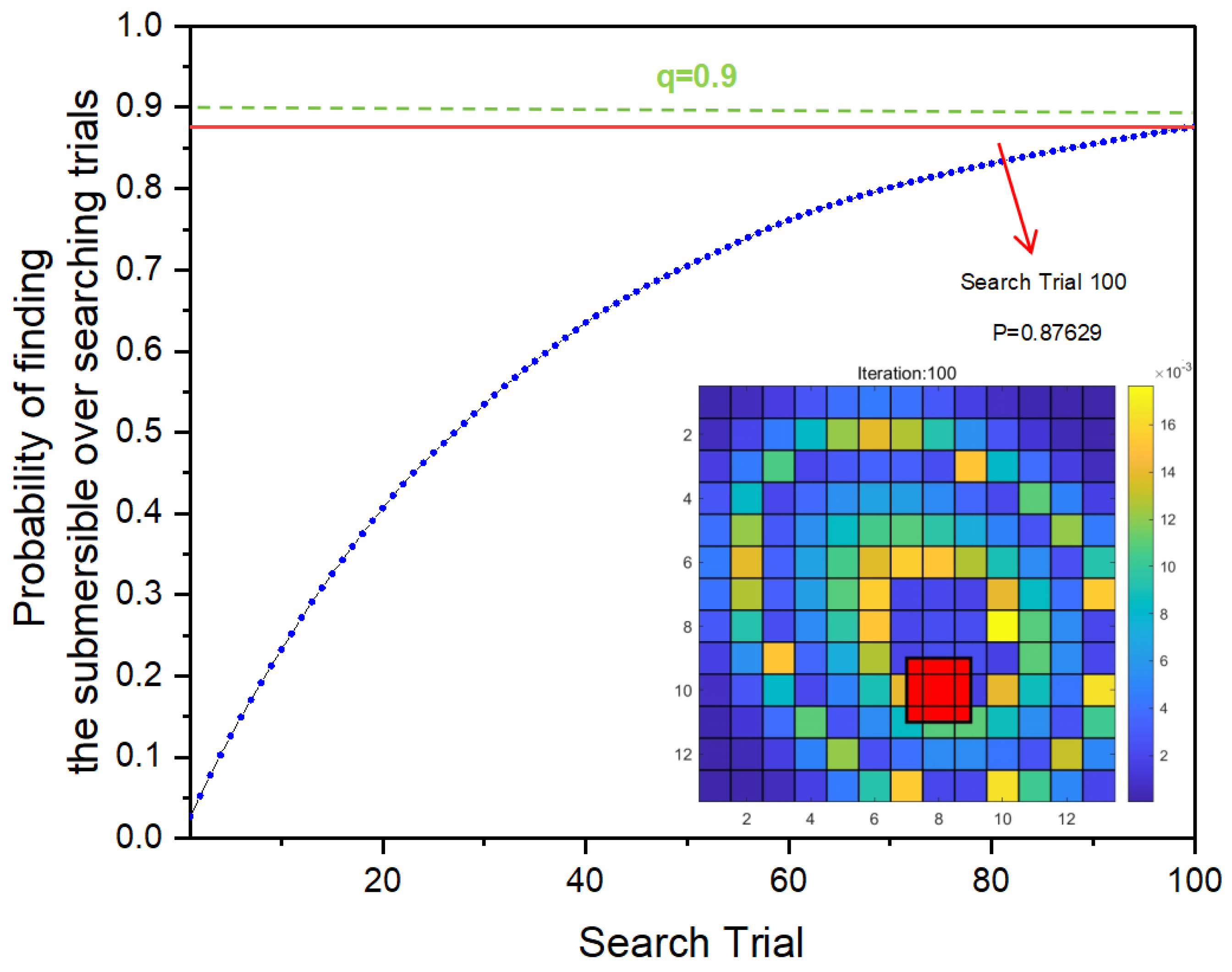
Here the q is set to be 0.9. The probability of finding the submersible over searching trials will finally approach q.
Table 3.
Probability of finding the submersible.
| Searching trial | 20 | 40 | 60 | 80 | 100 |
| P() | 0.4065 | 0.6352 | 0.7611 | 0.8309 | 0.8763 |
4. Extrapolation
The models presented earlier need to be adapted to account for varying environmental conditions and extended for the detection of multiple submersibles in close proximity. As an example, we consider the Caribbean Sea.
4.1. Seawater Density in the Caribbean Sea
According to oceanographic data, the seawater density in the Caribbean Sea remains relatively consistent, ranging from 1023.5 to 1024 [?]. In contrast to previous models where the function was employed to represent seawater density, the function is not suitable for the Caribbean Sea. Therefore, we approximate seawater density using a linear function based on the minimum riverbed elevation:
where is the maximum seawater density, and is the seawater density at the surface.
Figure 10.
Probability of finding the submersible over searching trials.
4.2. Warning and Obstacle Avoidance System for Multiple Submersibles
To enable multiple submersibles to operate safely within the same maritime area, we have implemented a warning and obstacle avoidance system. The warning distance between two submersibles is denoted as .
Figure 11.
Schematic diagram of obstacle avoidance principle.
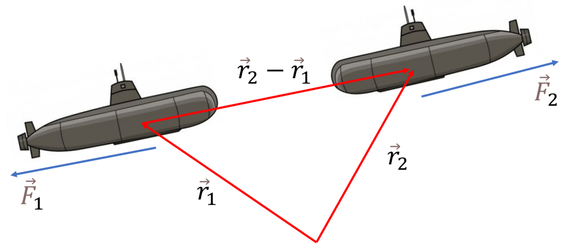
Considering two submersibles with trajectories and , respectively, the submersibles will adjust their propulsion forces whenever their predicted trajectories approach a dangerous proximity, i.e., . The submersibles adjust their paths while returning to their neutral buoyancy levels to avoid collision:
Figure 12.
Comparisons of submersible trajectories in the Caribbean Sea.
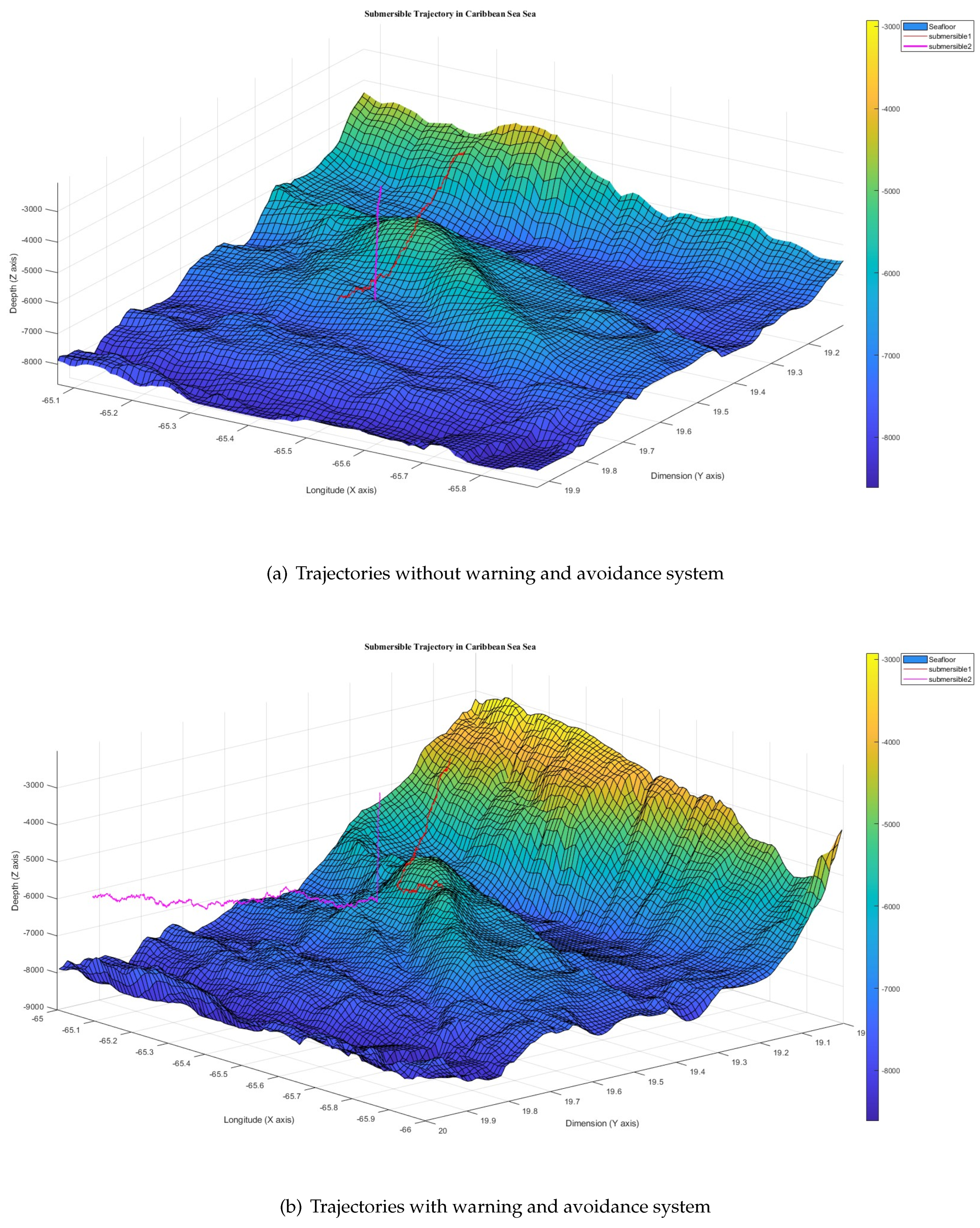
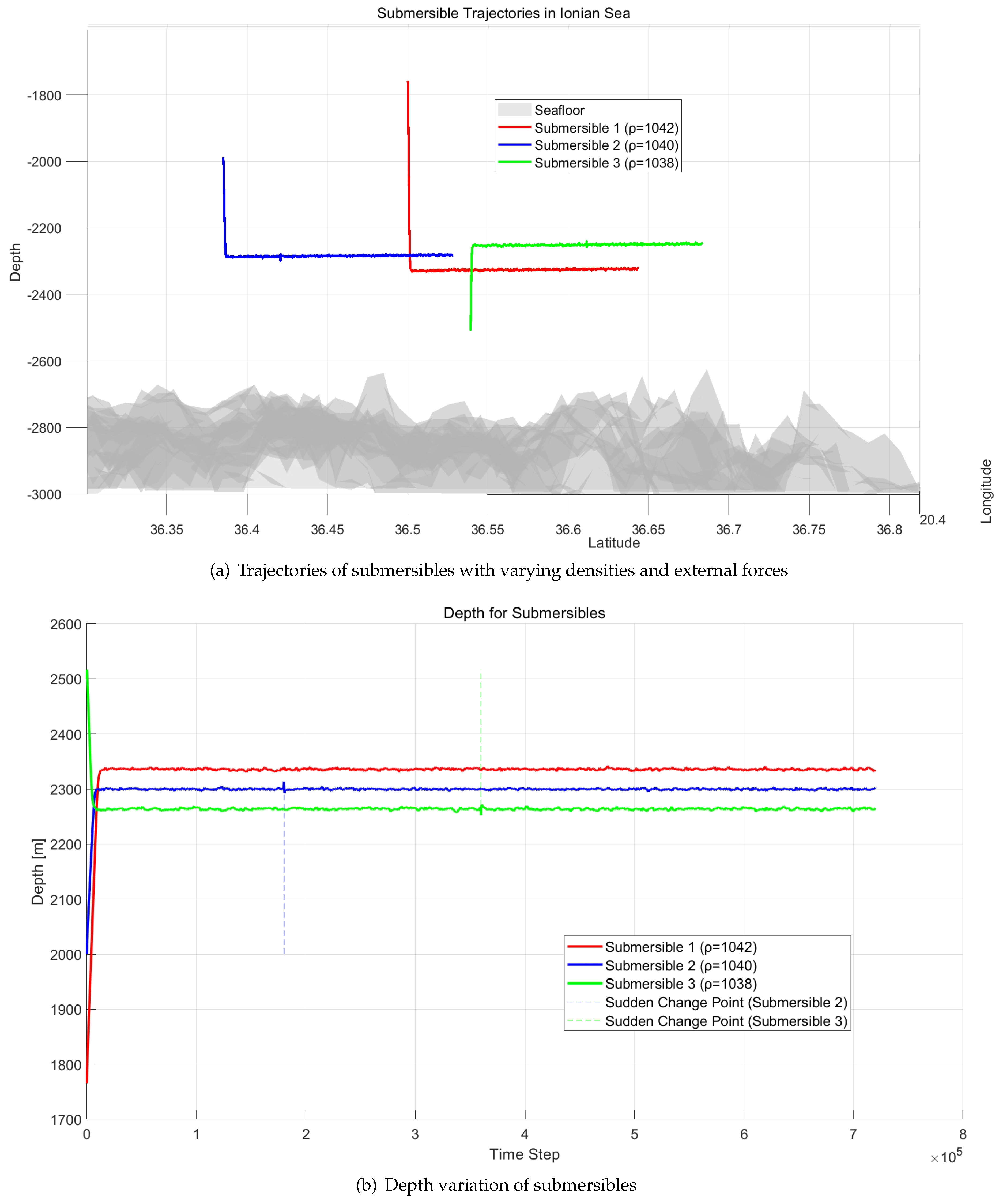
Figure 13(a) illustrates the trajectories of submersibles with different densities under external forces, while Figure 13(b) depicts the depth variation over time. The densities of the three submersibles are 1.38, 1.40, and 1.42, respectively.
The highlighted regions indicate moments when the submersibles were influenced by sudden external forces, such as rapid ocean currents, which caused a temporary deviation from their neutral buoyancy levels. Despite these disturbances, the submersibles quickly returned to their original buoyancy level, demonstrating the robustness of the model. Thus, the model exhibits stability in response to changes in density and short-term external forces, both over short and long time periods.
5. Reliability Analysis
In evaluating the reliability of the model, it is important to consider the assumptions made to simplify the model while ensuring it remains robust enough to provide useful insights in realistic scenarios. The assumptions provide a foundation for the model’s structure and allow for effective simulation under various conditions. Below is an analysis of the reliability of the model based on the key assumptions:
5.1. Assumptions and Their Impact on Reliability
-
The shape and density of the submersible remain unchanged underwater.Impact on Reliability: This assumption simplifies the model by treating the submersible as a rigid object, unaffected by external pressures. In reality, while extreme water pressure could potentially cause minor deformations, the materials used in submersibles are generally designed to withstand these conditions. By ignoring minor shape deformations, we prioritize model simplicity without sacrificing significant accuracy, making this assumption both reasonable and supportive of model reliability.
-
The density of seawater is influenced only by underwater depth.Impact on Reliability: By considering seawater density as dependent solely on depth, we eliminate the need to account for small changes in density caused by variations in longitude and latitude. This assumption holds because vertical movement significantly impacts the submersible’s buoyancy, while lateral movement over short distances has a negligible effect. This allows the model to focus on the primary variable—depth—thus increasing computational efficiency without compromising reliability for short timeframes and localized areas.
-
Two distinct scenarios are assumed after losing communication: mechanical defect or no defect.Impact on Reliability: Simplifying the analysis to two scenarios—either the submersible continues with unchanged propulsion or propulsion ceases due to a mechanical defect—provides a straightforward framework for determining the submersible’s trajectory after losing communication. While other failure modes could exist in reality, this binary distinction allows the model to focus on the most critical outcomes, enhancing reliability in failure prediction without introducing unnecessary complexity.
5.2. Analysis of Model Reliability Based on Assumptions
-
Structural Stability of the Submersible:The assumption that the submersible’s shape and density remain constant is integral to predicting reliable movement patterns underwater. Ignoring minor deformations caused by water pressure ensures that the model does not get bogged down by unnecessary complexities while maintaining realistic trajectory predictions. Given the robust materials used in submersibles, this assumption does not significantly reduce the model’s reliability.
-
Seawater Density and Depth Considerations:The assumption that seawater density is only affected by depth simplifies the buoyancy calculation, which is crucial for predicting vertical movement. Because vertical movement has a more pronounced effect on submersible buoyancy compared to lateral movement, the model remains highly reliable in predicting submersible depth changes. While minor fluctuations in density based on geographic location are disregarded, this does not diminish the model’s ability to operate in small to medium-scale geographic areas over short periods.
-
Failure Scenario Assumptions:The assumption of only two post-communication loss scenarios—continued propulsion or mechanical failure—enables a clear focus on the most likely outcomes. This binary framework is well-suited for simulating search and rescue operations. However, the model could be enhanced by incorporating more detailed failure modes, such as partial propulsion or sensor malfunctions. Nonetheless, the assumption allows for an efficient initial response framework and enhances the model’s reliability in the early stages of submersible tracking.
5.3. Overall Model Reliability
Based on these assumptions, the model remains reliable under typical operational conditions, particularly when used for short-duration missions or localized tracking of submersibles. By focusing on primary variables such as depth, buoyancy, and mechanical failures, the model provides robust predictions while maintaining computational simplicity.
Additional reliability could be gained by refining the failure scenarios or incorporating more real-world
6. Conclusions
In this paper, we presented a comprehensive mathematical model for enhancing submersible safety, focusing on location prediction, emergency procedures, and operational robustness. We developed and integrated models, including the Seawater Density Model, Submersible Mechanical Model, Bayesian Searching Model, and Extended Kalman Filter, to simulate and analyze the movement of submersibles in marine environments. These models were extended to different scenarios, such as the Caribbean Sea, and were equipped with a warning and obstacle avoidance system to manage multiple submersibles.
The reliability of the model was examined through sensitivity analysis, demonstrating its adaptability to varying environmental conditions and sudden external forces. The model’s accuracy was further improved through the incorporation of uncertainties using an Extended Kalman Filter, Gaussian Mixture Model, and Background Impulse Kalman Filter, ensuring precise trajectory prediction.
Incorporating both theoretical and practical elements, the model provided efficient search procedures through Bayesian search techniques, minimizing the time needed to locate a missing submersible. The study highlights the significance of simplifying assumptions while maintaining reliability, and the overall robustness of the models ensures their applicability across a range of marine environments and operational challenges.
Future improvements can focus on refining the failure scenarios, increasing the precision of real-time data inputs, and expanding the model to accommodate more complex oceanographic and mechanical dynamics.
References
- ArcGIS. Latitude and Longitude Data. Accessed: 2024-10-19. 2024. url: https://www.arcgis.com/index.html.
- Tan Dalin, Zhou Jifu, and Wang Xu. “Study on the Ocean Density Profile Model and Its Applicability”. In: Advances in Marine Science 39 (2021), pp. 30–36. issn: 1671-6647. [CrossRef]
- Kristofer D¨o¨os et al. “The World Ocean Thermohaline Circulation”. In: Journal of Physical Oceanography 42.9 (2012), pp. 1445–1460. url: https://journals.ametsoc.org/view/journals/phoc/42/9/jpod-11-0163.1.xml. [CrossRef]
- Xuxiang Fan et al. “A Background-Impulse Kalman Filter With Non-Gaussian Measurement Noises”. In: IEEE Transactions on Systems, Man, and Cybernetics: Systems 53.4 (2023), pp. 2434–2443. [CrossRef]
- NASA Earthdata Search. Altitude Data. Accessed: 2024-10-19. 2024. url: https://search.earthdata.nasa.gov/search.
- Guoqing Wang, Ning Li, and Yonggang Zhang. “Distributed maximum correntropy linear and nonlinear filters for systems with non-Gaussian noises”. In: Signal Processing 182 (2021), p. 107937. issn: 0165-1684. [CrossRef]
- Zhixia Xie. “Research on Target Localization and Tracking Method Based on Multiple Autonomous Underwater Vehicles”. MA thesis. Zhejiang University, 2023.
- Kuilin Yuan, Hongyi Jin, and Wei Chai. “Development of a new spectral method for fatigue damage assessment in bimodal and trimodal Gaussian random processes”. In: Ocean Engineering 267 (2023), p. 113273. issn: 0029-8018. url: https://www.sciencedirect.com/science/article/pii/S0029801822025562. [CrossRef]
Figure 2.
Dynamic analysis of submersible.
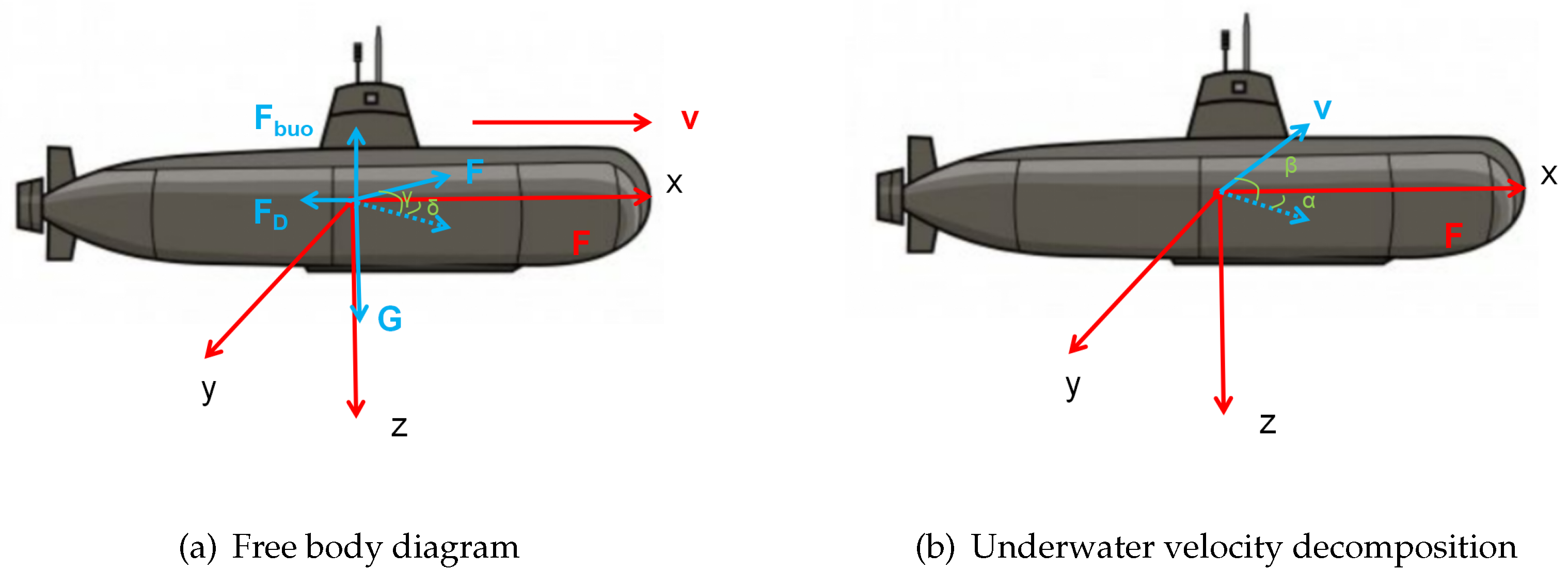
Figure 3.
Seabed depth in the Ionian Sea.
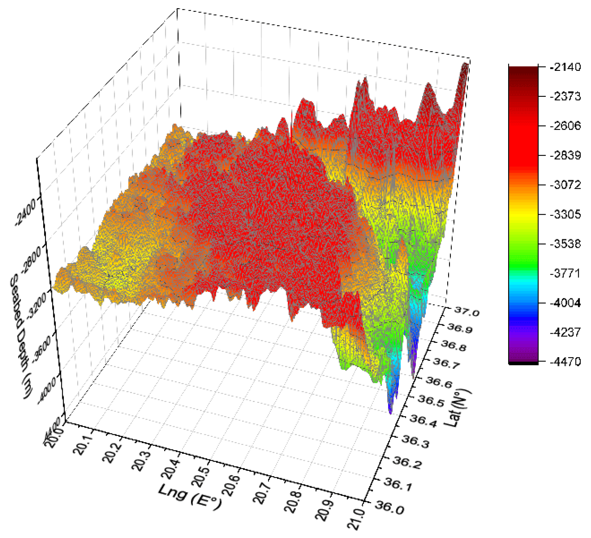
Figure 4.
Simulated trajectory of submersible (hit the seabed).
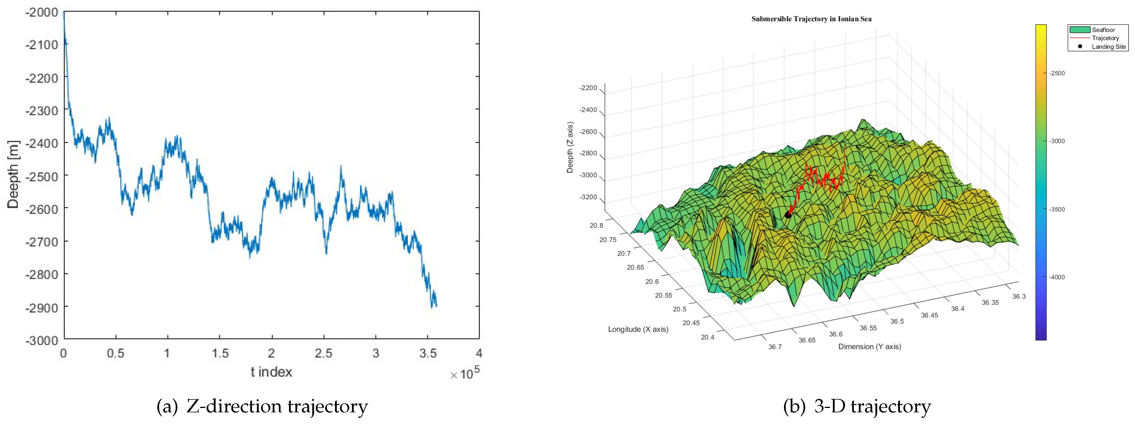
Figure 5.
Simulated trajectory of submersible (levitating).
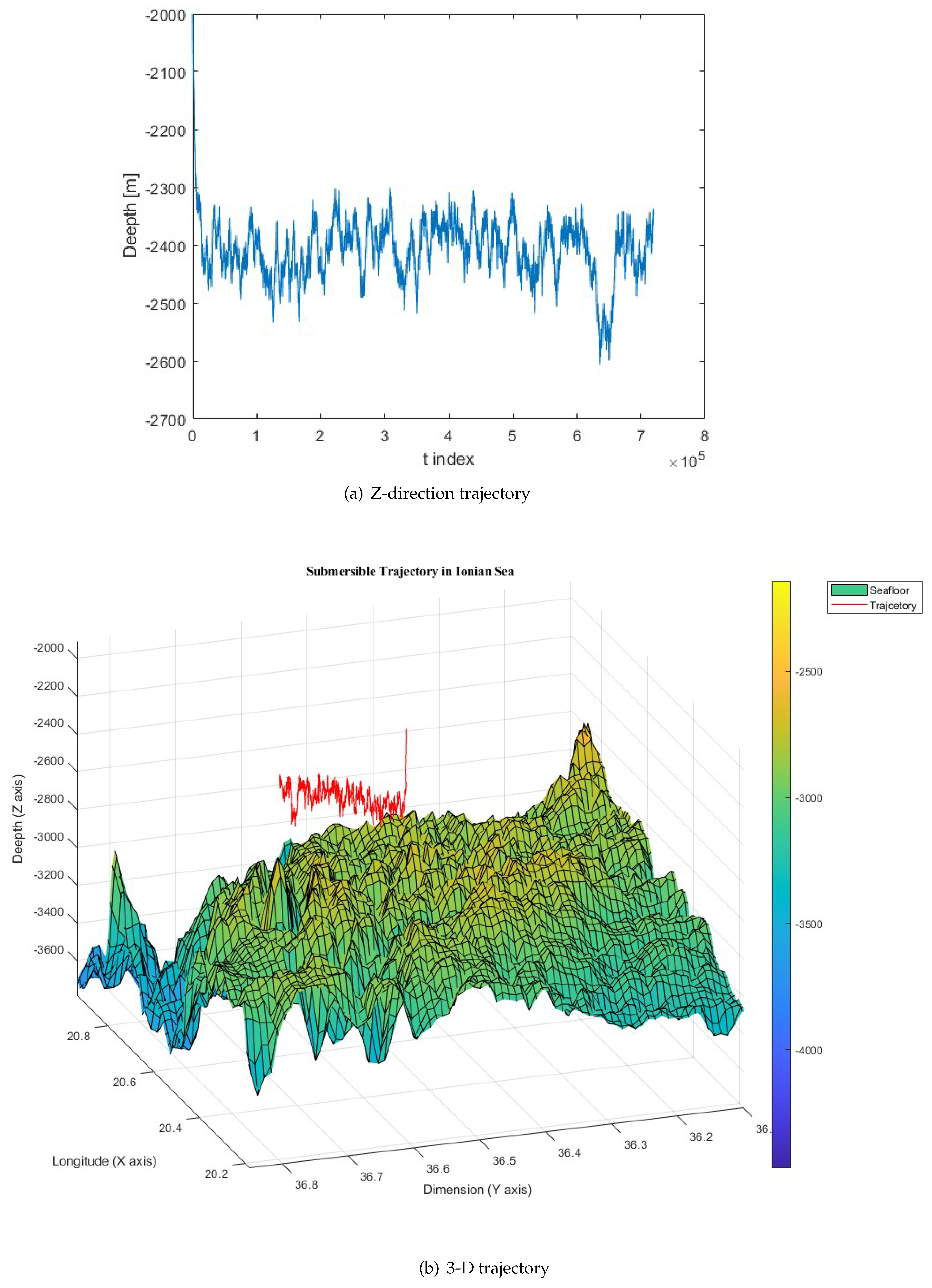
Figure 8.
Discretization of searching grids and renewing possibilities.
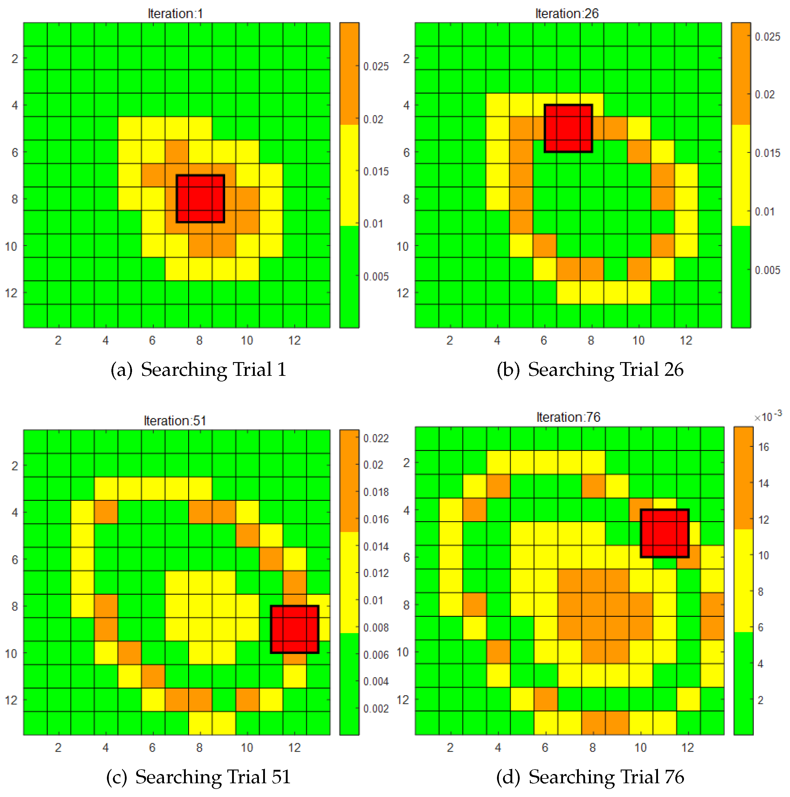
Figure 9.
Discrete Bayesian searching with submersible trajectory, which looks like searching in avocado.
Figure 9.
Discrete Bayesian searching with submersible trajectory, which looks like searching in avocado.
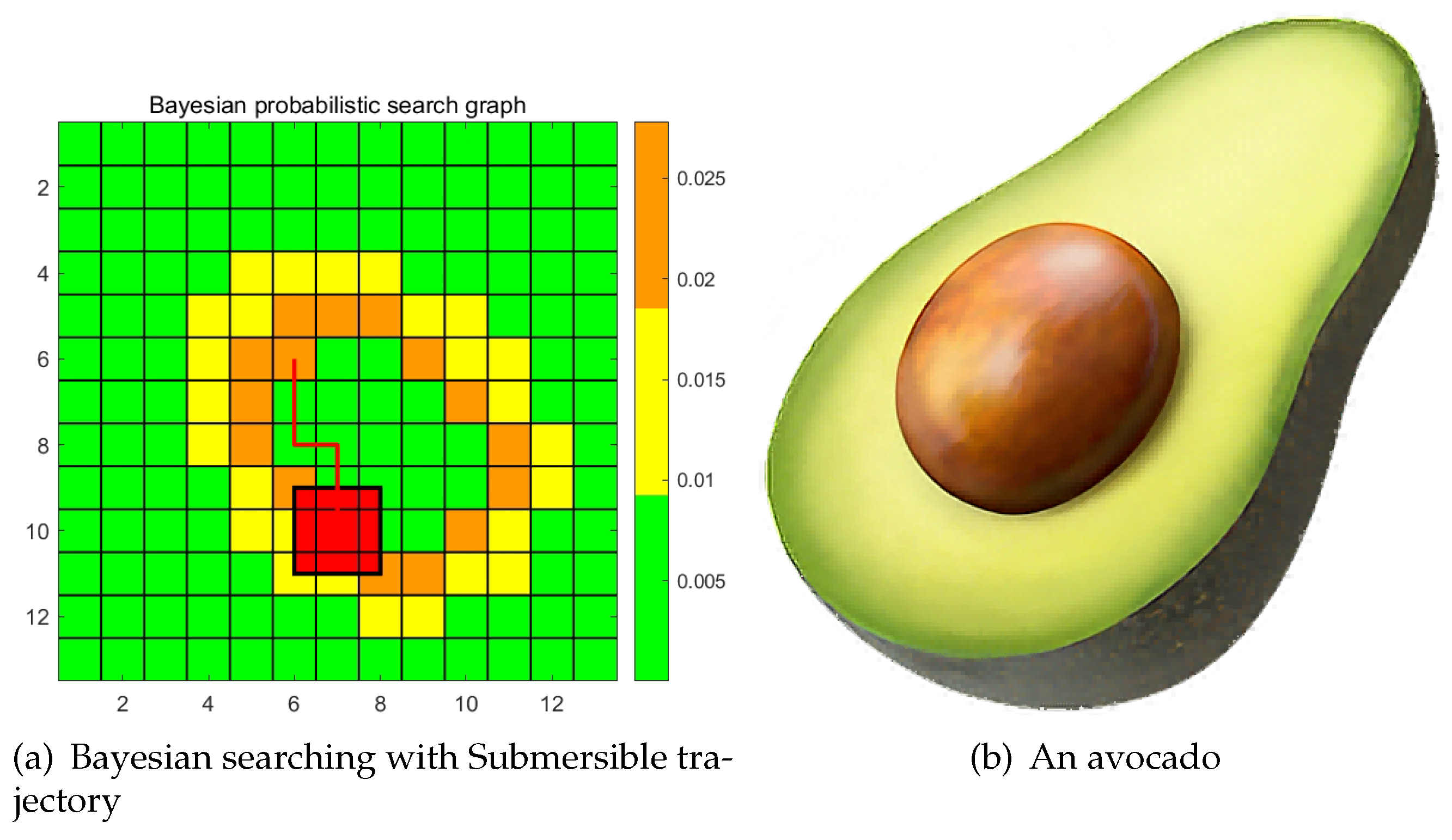
Figure 13.
Trajectories and depth variation in sensitivity analysis.
Disclaimer/Publisher’s Note: The statements, opinions and data contained in all publications are solely those of the individual author(s) and contributor(s) and not of MDPI and/or the editor(s). MDPI and/or the editor(s) disclaim responsibility for any injury to people or property resulting from any ideas, methods, instructions or products referred to in the content. |
© 2024 by the authors. Licensee MDPI, Basel, Switzerland. This article is an open access article distributed under the terms and conditions of the Creative Commons Attribution (CC BY) license (http://creativecommons.org/licenses/by/4.0/).
Copyright: This open access article is published under a Creative Commons CC BY 4.0 license, which permit the free download, distribution, and reuse, provided that the author and preprint are cited in any reuse.


