
Submitted:
27 January 2026
Posted:
28 January 2026
You are already at the latest version
Abstract
Irreversible evolution with partial retention of history appears in systems that build structure, from cosmological clustering and galaxy evolution to biological inheritance and optimization dynamics in machine learning. In each field, "memory'' is introduced in different language and with different objects, which makes it hard to compare mechanisms, to identify what is minimal, or to formulate falsifiable cross--domain predictions.This paper presents a compact axiomatic and effective--action foundation for the \emph{Infinite Transformation Principle} (ITP): a class of systems that (i) exhibit monotone structural growth before saturation, (ii) respond to a finite causal segment of their history, (iii) saturate in structural capacity, and (iv) include a stabilizing long--wavelength feedback. Under these assumptions a generic ITP system admits, up to smooth reparameterization and field redefinitions, a representation governed by seven parameters \[ (\alpha, m, S_{\max}, \Delta, \beta, \mu, \eta), \] grouped into growth, memory--horizon, and memory--response couplings. These parameters arise from a minimal localizable nonlocal action (equivalently, an auxiliary--field formulation) and make explicit the conditions under which a single--timescale exponential kernel is the unique stable one--parameter memory kernel.The paper then defines the seven--dimensional parameter manifold $\MITP$, constructs simple dimensionless invariants for cross--domain comparison, and spells out what must be reported to claim empirical constraints on memory: kernel choice, structural source, parameter combinations, null tests, and data/likelihood details. A separate simulation paper derives an exponential drag kernel from TNG300--1 by coarse--graining $\sim 50\,{\rm Mpc}/h$ domains and measuring the response of an expansion--rate deviation to a velocity--dispersion source. Here that result is used as an explicit example of how the abstract ITP parameters map onto a concrete kernel measurement, and how short, Gyr--scale domain memory can coexist with a much longer, effective memory horizon in background cosmology fits.The result is a "parameter handbook'' for memory--bearing irreversible dynamics: it states clearly what is assumed, what is minimal, what is identifiable, and what would falsify the framework in real data.
Keywords:
infinite transformation principle (ITP)
; structural memory
; coarse-graining kernel
; cosmological kernel
; TNG300
; TNG50 simulations
; scale dependence of memory
; memory horizon
1. Introduction
Many structure–building systems are neither well described by purely Markovian dynamics nor by conservative Hamiltonian evolution. They are history–sensitive, saturating, and they exhibit an arrow of time in their structural degrees of freedom. In cosmology, structure grows from small initial perturbations and retains long–lived correlations. In biology, inheritance couples present fitness to a lineage record. In machine learning, optimization procedures explicitly use information from multiple past steps and often face capacity– and regularization–induced saturation.
The problem is not the lack of memory models; it is the fragmentation. Different fields define memory with different objects (kernels, hidden states, heredity operators, delayed terms). That makes it difficult to ask basic questions:
- What is the minimal structure required to represent finite causal memory with saturation?
- How many independent parameters are actually needed to describe the memory sector?
- Which combinations are identifiable in a given dataset?
- What would falsify a claimed memory effect?
The Infinite Transformation Principle (ITP) is a domain–agnostic description of a class of systems with irreversible structural growth and finite memory. It is deliberately modest. It does not try to replace domain–specific microphysics. Instead it:
- states explicit axioms (Sec. 2);
- derives the minimal parameterization consistent with those axioms (Sec. 4);
- defines a parameter manifold and dimensionless invariants (Sec. 5);
- specifies what must be reported to claim empirical constraints (Sec. 7);
- connects this abstract structure to a concrete kernel measured in TNG300–1 (Sec. 8).
A separate paper, Virialisation as Viscosity: Deriving the ITP Cosmological Memory Kernel from TNG300, takes a first step toward a simulation–based derivation of the cosmological kernel. It coarse–grains TNG300–1 into domains, constructs a velocity–dispersion structural source and an expansion–rate deviation, and measures a short, negative exponential kernel with a characteristic time and integrated drag strength . The present paper provides the theoretical scaffold within which that result, and future observational tests, can be placed.
2. Axioms and Volterra Structure
The ITP is defined as a model class for systems that grow structure irreversibly, respond to a finite causal history, and saturate.
Definition 1
(ITP axioms). A system belongs to the ITP class if there exists a scalar structural measure and a memory functional such that:
- A1.
-
Irreversible structural growth. For accessible states prior to saturation,for almost all t in the pre–saturation regime. This encodes a structural arrow of time.
- A2.
- Causal path dependence. Evolution depends on a functional of the recent past; specifically, the dynamics can be written with constructed from through a causal kernel.
- A3.
- Finite memory horizon. The memory kernel is causal ( for ), integrable, and decays on a characteristic timescale Δ:
- A4.
- Saturation. Structural growth is capacity–limited:
- A5.
- Contractive long–wavelength response. Accumulated memory induces a stabilizing (negative–definite) correction to coarse/long–wavelength modes of the background evolution. In linearized form, the memory sector does not introduce new runaway directions in the effective response operator.
Axioms A1–A4 encode irreversibility, finite history, and bounded complexity. Axiom A5 is the stability axiom. Without it, one can build memory models that fit anything by blowing up. Here it is made explicit and testable: it implies sign constraints on the effective couplings in the background sector (Sec. 3).
Axiom A5 is a statement about the spectrum of the coarse–grained response, not about the sign of any single empirical correlation such as in a given dataset. Effective couplings can change sign when one moves between structural regimes inside . The “double flip” seen in galaxy data—where depth–memory and stability–regeneration correlations change sign between low– and high–stability populations—is therefore compatible with A5: the underlying response remains contractive, while its observable projections depend on where the system sits in parameter space.
2.1. From Coarse–Graining to a Causal Memory Kernel
Let denote the resolved structural variable and let denote unresolved degrees of freedom. At microscopic level one has
with appropriate boundary conditions. Eliminating X generates an exact history dependence in the reduced equation for S. Under mild assumptions (causality, bounded response) the reduced dynamics can be written in Volterra form
where:
- is the Markovian part of the dynamics;
- encodes external forcing or boundary driving;
- is an effective source constructed from past states;
- is a causal memory kernel.
A convenient representation introduces an auxiliary memory field obeying a linear relaxation equation,
with a stable linear operator. The solution can be written as
where is the retarded Green function of . Identifying
turns Eq. (5) into the standard ITP form: the kernel is the causal propagator of a stable memory channel, not an arbitrary function.
The minimal stable choice for is a one–pole relaxation operator,
which yields the exponential kernel
with the Heaviside function enforcing causality. This kernel is not chosen for convenience; within the one–timescale, stable, localizable sector it is the unique choice.
For interpretation it is useful to define an operational memory horizon as the lookback time that contains a fixed fraction q of the kernel weight:
For the exponential kernel,
so a fitted horizon directly maps onto the relaxation time .
In cosmology the same structure appears when nonlocal terms in an infrared effective action are localized with auxiliary fields and retarded boundary conditions. After a cosmological reduction, one obtains history integrals of exactly the form in Eq. (5). In that sense the ITP kernel is an effective, causal response function rather than a handcrafted delay.
The ITP does not claim to identify the unique microscopic origin of K. It claims something narrower and testable: data can be used to decide whether a finite, causal memory term is preferred over a Markovian closure, and if so, which small family of stable kernels is supported. The exponential kernel represents the minimal single–timescale case; multi–timescale or oscillatory kernels live outside the seven–parameter minimal sector.
3. Localizable Effective Action and Couplings
Axioms A2–A3 motivate a history integral of Volterra type. A standard way to avoid pathological nonlocalities is to introduce an auxiliary field whose equation of motion generates the kernel as a Green’s function. This yields a localizable nonlocal model: nonlocal in the reduced description, local in an extended state space.
3.1. Memory Functional and Localization
Define the memory functional
For the exponential kernel
the same object obeys the first–order local equation
This representation makes the model implementable and numerically stable. It also makes initial conditions explicit.
3.2. Effective Action and Memory Couplings
Let denote the system degrees of freedom (fields, coordinates, state vector). The ITP class is described schematically by an effective action
with the memory constraint enforced either by substituting Eq. (13) or by adding a Lagrange–multiplier form of Eq. (15). Here:
- is a growth–and–saturation potential (Sec. 4.1);
- couples memory to the “background” effective potential via (stiffness/deformation);
- couples the memory rate to a kinetic structure (history–weighted dissipation / kinetic mixing);
- couples memory to an external quadratic sector (mass–like shift, cross–sector influence).
Axiom A5 translates into sign/inequality constraints on the combinations of that feed into the long–wavelength sector: the effective correction to the background potential must be negative–definite in the appropriate variables so that memory feedback is contractive, not explosive. These constraints must be stated explicitly when fitting data.
4. Seven Parameters: Derivation, Minimality, Identifiability
4.1. Structural Growth Law
Axioms A1 and A4 require monotone growth toward a finite ceiling. A minimal smooth form is a time–weighted logistic equation
with solution
The three parameters are interpretable across domains: sets production amplitude, m encodes temporal acceleration or deceleration of production, and is the carrying capacity.
This form is not unique, but it is minimal: it is the lowest–parameter smooth saturating monotone law with explicit time–weighting. Alternative saturating families (Gompertz, generalized logistic, Hill–type) can be used in specific domains, but then the mapping back to must be stated.
4.2. Memory Horizon as a Unique Scalar Timescale
Given a causal, integrable kernel , define the characteristic memory timescale by the ratio of moments
when these integrals exist. This scalar is invariant under time translation and provides a model–independent notion of “center–of–mass” memory age.
Theorem 1
(Uniqueness of a one–parameter stable memory horizon). Assume is causal, integrable, nonnegative, and generated by a stable one–pole linear relaxation operator on an extended state space. Then is proportional to an exponential kernel and the model contains exactly one memory–horizon parameter .
The exponential kernel in Eq. (10) is therefore the unique minimal kernel in the one–timescale, localizable sector. Multi–timescale kernels, fractional operators, or oscillatory kernels introduce additional parameters and live outside the seven–parameter minimal family.
4.3. Minimal Seven–Parameter Representation
Theorem 2
(Seven–parameter minimal representation). Consider the ITP class restricted to: (i) a three–parameter smooth saturating growth family for , (ii) a one–parameter stable causal memory kernel generated by a localizable relaxation operator, and (iii) leading–order (lowest–derivative) memory couplings in an effective–action expansion. Then any such system admits a representation governed by exactly seven parameters
up to smooth reparameterization and field redefinitions. Under the same restrictions, no representation with fewer than seven parameters can satisfy A1–A5 while maintaining background stability and non–degenerate identifiability of memory effects.
Sketch.
- A1 and A4 require saturating monotone growth; the minimal three–parameter family provides .
- A2–A3 with a one–pole stable kernel introduce a single timescale .
- A5 demands at least one stabilizing background correction and one independent perturbation–level (dissipative / kinetic) correction at leading derivative order, giving .
- A cross–sector quadratic coupling introduces and is required if the model is to be compared across domains.
- Under the stated restrictions, none of these parameters can be removed by rescaling t, shifting S, or redefining without either violating an axiom or collapsing the model back to a Markovian limit.
□
Phase structure in .
Although Theorem 2 characterises a single connected parameter manifold, empirical systems can occupy different “phases” within it. In those phases, effective couplings—for example the response of memory to depth, or regeneration to stability—can change sign as structural variables approach their saturation scales. The processor–to–reservoir transition seen in galaxy evolution is best read as a trajectory in that crosses a surface where these effective responses change sign while Axioms A1–A5 remain valid.
Corollary 1
(Operational necessity tests). In the restricted minimal model:
- or removes structural production (violates A1).
- removes saturation (violates A4).
- collapses memory to instantaneous response (Markovian reduction of A2–A3).
- removes memory feedback on the background (violates A5 in the background sector).
- removes independent memory–induced damping (degenerates perturbation response).
- removes the leading cross–sector coupling channel (collapsing universality claims to a single–sector phenomenology).
5. The ITP Parameter Manifold and Dimensionless Invariants
Definition 2
(ITP parameter manifold).
Topologically, (semi–bounded, non–compact). For cross–domain comparison, raw parameters are less useful than dimensionless invariants.
5.1. Dimensionless Invariants
A convenient nondimensionalization uses the memory timescale and the capacity . One minimal invariant set is
Other invariant sets are possible; what matters is that at least one such set is reported whenever systems are said to “share the same ITP parameters.”
5.2. Schematic Phase Regions
Figure 1 is an illustrative schematic, not a literal embedding of seven dimensions.
6. Universality: A Careful Dictionary Across Domains
Operationally, universality means that the same reduced equations can fit observables in different domains after an explicit mapping. The mapping is a hypothesis, not a trophy.

Table 1.
Illustrative interpretations of ITP parameters across domains.
| Parameter | Cosmology | Biology | Machine learning |
|---|---|---|---|
| structure proxy (clustering / ordering) | complexity proxy (heritable structure) | performance / capacity proxy | |
| structural production amplitude | innovation / mutation supply | base learning–rate scale | |
| m | time–weighting of production | epoch–dependence of selection | schedule exponent |
| effective max structure | complexity ceiling (constraints) | model capacity ceiling | |
| effective memory / coherence time | inheritance persistence time | momentum decay / context window | |
| background coupling (history to mean) | selection / feedback strength | regularization stiffness | |
| damping of fluctuations | stabilizing drag / robustness | gradient damping / regularization | |
| coupling to other sectors | environment coupling | transfer / multi–task coupling |
For any two domains A and B, a universality statement requires:
- explicit observables mapped to and/or ;
- a fitted invariant set with uncertainties;
- model comparison against domain–standard baselines;
- at least one falsifier: a result that would kill the mapping.
6.1. Mesoscopic Example: Galaxy Homeostasis and the Stability Gate
Galaxy evolution provides a mesoscopic example where the abstract coordinates acquire explicit observational counterparts. In a recently proposed description, a galaxy at fixed epoch is characterized by a compact state vector
where H is a depth or energy proxy (e.g. stellar velocity dispersion probing the potential well), S is a stability proxy (a structural maturity coordinate), M is a chemical memory proxy (mass–residual metallicity or an analogous quantity), and R is a regeneration proxy (specific star formation rate, averaged over a finite time window).
In this language, acts as a slow structural variable, acts as a coarse memory of past flow, and tracks the current rate at which new material is incorporated. The ITP axioms apply: galaxies grow structure irreversibly in S, they retain partial memory in M, and they do not grow indefinitely.
Empirically, galaxies separate into two regimes across a stability threshold . Below the threshold, in an “infant” regime, deeper potential wells correlate with reduced residual memory at fixed mass, and increased stability correlates with reduced regeneration. Above the threshold, in an “adult” regime, both couplings flip sign: deeper wells now support higher chemical memory, and greater stability supports higher regeneration. This “double flip” is consistent with a transition from a processor–like phase, where energy and structure act to erase detailed history, to a reservoir–like phase, where the same variables act to retain and exploit it.
Within the present framework, this behaviour is naturally interpreted as motion within from a region where the effective response of to is dominantly erosive, to a region where the response is dominantly retentive and regenerative, while global contractivity and finite–memory conditions remain satisfied. The adult regime behaves homeostatically: depth, structure, memory and regeneration form a feedback loop that resists both dilution and runaway collapse.
The two sign inversions can be expressed as a transition from an effectively Markovian to a history–dependent regime. In the infant population,
so the current memory state carries little extra predictive power beyond depth and stability at fixed environment . Adult systems instead satisfy
so the current memory state becomes a meaningful predictor of future behaviour. In this reading, infant galaxies behave as fast processors, adult galaxies behave as reservoirs, and the environment acts as a modulator rather than a master switch.
7. Empirical Interface: What Must Be Reported
The seven parameters define the minimal model class. Real datasets only constrain some combinations, and constraints are always conditional on a choice of structural proxy, kernel family, and likelihood. This section states the basic reporting requirements.
7.1. Cosmology: Parameter Identifiability and Correlations
In a minimal cosmological implementation, one typically works with a five–parameter extension of CDM for background and linear growth:
where is a memory amplitude parameter, is the memory horizon, and is a late–time growth amplitude that renormalizes the linear prediction. The combinations are embedded in how and enter the Friedmann and growth equations.
A representative joint fit to and shows the following qualitative correlation structure:
The strongest degeneracy is the familiar geometric one between and , already present in CDM. A second strong relation appears between and : more matter can be offset by a lower growth amplitude. Both are standard.
The new behaviour lies in the memory sector. The anti–correlation between and shows that part of what is usually attributed to “today’s expansion rate” in a Markovian model can be expressed as accumulated memory in a non–Markovian one. By contrast, and are nearly uncorrelated, and shows only weak correlations with all other parameters. The strength of memory and its characteristic timescale are effectively independent degrees of freedom at this level.
This correlation structure is what one wants: the ITP extension retains the known degeneracies of background cosmology, introduces a memory amplitude that trades explanatory weight with , and adds a memory horizon that acts as a genuinely new temporal parameter rather than a disguised rescaling.
7.2. Reproducibility Checklist
Any claimed cosmological constraint on ITP parameters should report:
- datasets and likelihoods (names, versions, priors, nuisance treatment);
- the full parameter vector sampled, including standard cosmological parameters;
- the mapping equations: how S and M enter background and perturbations;
- the kernel choice and whether multi–timescale kernels were tested;
- goodness–of–fit metrics (, Bayes factors if used);
- posterior predictive checks on withheld statistics;
- at least one null test designed to fail if the signal is a reconstruction artifact.
If is normalized (for example ), that choice must be stated so that and can be interpreted correctly.
7.3. Nonlinear Memory Signatures: Phase Correlations
Claims of a nonlinear “phase–correlation angle” or related statistic should specify:
- the fields analysed (maps, masks, component separation choices);
- the estimator definition (phases of what decomposition, multipole or scale ranges);
- the null ensemble generation (number of simulations, systematics included);
- look–elsewhere correction if multiple angles or ranges were scanned;
- robustness to known systematics (beam, noise anisotropy, masking).
Without these, any quoted p–value is decoration, not a result.
8. Example: Memory–Horizon Scaffolds and Simulation Kernel
This section shows how the abstract ITP structure connects to two concrete cases:
- a scaffold fit of the background memory horizon from data;
- a simulation–level kernel measurement from TNG300–1 on domains.
The first illustrates how little current data can say about in isolation. The second shows how the same formalism recovers a short, negative exponential kernel at the domain level.
8.1. Memory–Horizon Fits to Data (Scaffold Only)
A grid–based scaffold fit of the ITP memory horizon has been applied to a cleaned compilation of measurements, using:
- an exponential memory kernel in the background closure;
- a linear baseline plus a minimal memory template in lookback time;
- a fiducial CDM redshift–to–time mapping.
All results in this subsection are scaffolds: they validate the pipeline, but they are not final parameter inferences.
For the full compilation ( points, combining cosmic chronometers and BAO), the log–likelihood as a function of increases toward the upper edge of the scanned range, with a maximum at the prior boundary,
and a best–fit log–likelihood of order
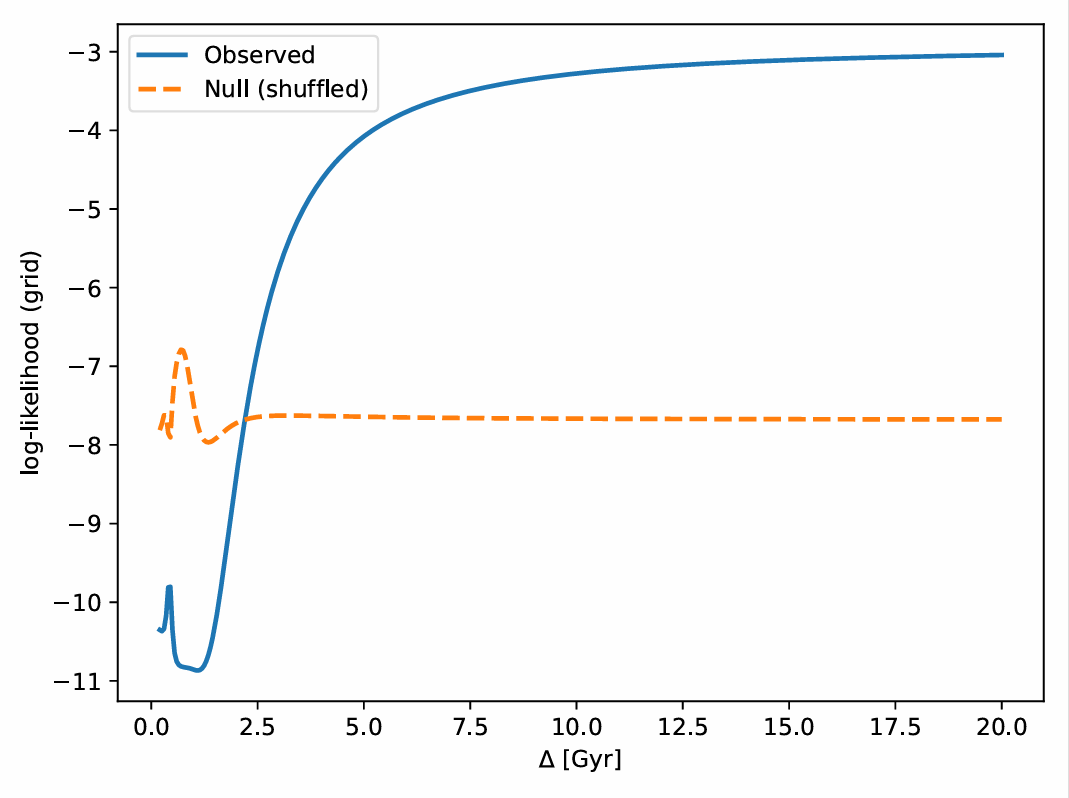
The maximum sitting at the prior edge indicates that the current data do not meaningfully constrain the memory horizon within this model: the data remain compatible with arbitrarily long effective memory over the tested range.
Figure 2 shows the normalized likelihood curve from this grid. A null test obtained by shuffling the values relative to redshift and refitting produces curves that look statistically similar (Figure 3). In other words, a preference for long can arise from chance alignment in sparse data under a flexible template. Until a full joint analysis with growth, lensing, or other probes is performed, and until stricter baselines are compared, the only honest statement is that alone does not identify .
8.2. TNG300 Domain Kernel and Scale–Dependent Memory
The companion paper on virialisation treats TNG300–1 as a laboratory for the ITP kernel. The simulation is coarse–grained into a regular grid of comoving domains, each of linear size . For ten snapshots between and , the analysis constructs:
- a structural sourcethe domain–averaged subhalo velocity–dispersion squared;
- an expansion–rate deviationin .
These two time series are related through a discrete Volterra relation of the form
with trapezoidal weights . For a single–exponential kernel
the best–fit parameters from the ten–snapshot series are
with a mean–squared error of order in the chosen units. A cross–check fit excluding the final snapshot yields and , leaving the integrated drag essentially unchanged. The sign of A is robustly negative. Given the convention
a negative A implies that increasing drives , so virialising structure acts as a viscosity: as domains heat up dynamically, the effective expansion rate is pulled below the Friedmann value.
Within the ITP language, this is a direct measurement of a short, local kernel on domains. Its timescale is of the same order as dynamical times in cluster environments, not of order . There is no contradiction with the long effective memory horizons allowed by fits; they live at different levels of coarse–graining:
- is a domain–scale kernel controlling how local virialisation drags the domain expansion.
- in the background closure is an effective horizon–scale summary of many such relaxation events, integrated across space and time.
A natural interpretation is that cosmological memory is scale–dependent. On cluster and supercluster scales, structure formation imprints a short, negative kernel whose width is set by local dynamical times. On horizon scales, the effective kernel seen by the background expansion is the cumulative imprint of many local drag events across a hierarchy of scales, leading to a long–range, non–Markovian drift in the effective Friedmann law.
The ITP parameter space is where these different levels meet. Both the TNG300 and TNG5 result shows that a negative, finite kernel emerges from explicit structure formation once the simulation is coarse–grained. The parameter–space paper tells you how to encode that kernel and its couplings as points and directions in , and how to keep the story consistent when you move from simulations to fits, to galaxy population statistics, and back.
9. Limitations and Extensions
A few obvious caveats:
- Kernel minimality is a restriction. Exponential memory is the minimal one–parameter stable kernel. Data may eventually demand multi–timescale or oscillatory kernels. Those live outside the seven–parameter minimal sector and carry extra parameters that must be earned.
- Choice of structural proxy. is a scalar proxy by design. In some systems structure is irreducibly vector– or field–valued. Extending ITP to multiple coupled structural measures is straightforward but increases parameter count and complicates identification.
- Identifiability vs. interpretation. The mapping from observables to is always a modeling choice. Constraints are on the reduced model, not on ontological “memory”.
- Dataset dependence. The correlation structure in Table 2 comes from a specific compilation and pipeline. Different compilations or priors can shift numbers while keeping the overall pattern.
10. Conclusions
This paper has presented the Infinite Transformation Principle as a minimal parameter framework for irreversible structural growth with finite causal memory and stabilizing feedback. The main result is not a striking numerical claim; it is a clean separation of:
- what is assumed (A1–A5);
- what follows mathematically (a seven–parameter representation in the restricted model class and a simple set of invariants);
- what must be shown empirically (identifiable parameter combinations, nonlinear signatures, and reproducible pipelines).
The TNG300 kernel measurement shows that a short, negative exponential kernel appears when a standard hydrodynamic simulation is coarse–grained into domains. The scaffolds show that background data alone are currently too weak to pin down an effective memory horizon. Galaxy population studies show a processor–to–reservoir transition consistent with a change of phase within . None of these, on their own, proves that the universe obeys ITP. Together they say something more modest and more useful: in order to talk about memory in cosmology and beyond, it should be done in a way that is explicit, minimal, and falsifiable, and should be honest about which parameters are actually constrained.
If the ITP framework survives contact with future data, it will be because it keeps those promises. If it fails, it should fail cleanly, under the falsifiers and reporting requirements spelled out above.
Notation and Conventions
| Structural entropy / scalar measure of accumulated structure | |
| Generic dynamical degrees of freedom (fields, state vector components) | |
| Memory functional (history–dependent auxiliary variable) | |
| Causal memory kernel, | |
| Memory horizon / characteristic memory timescale | |
| Intrinsic growth amplitude (structural production efficiency) | |
| m | Temporal scaling exponent (time–weighting of production) |
| Saturation capacity (finite structural ceiling) | |
| Memory–to–background coupling (potential deformation / stiffness) | |
| Dissipative coupling (history–weighted damping / kinetic mixing) | |
| Cross–sector coupling (mass–like shift from memory) | |
| Seven–dimensional ITP parameter manifold | |
| Dimensionless invariants for cross–domain comparison |
Conventions. Dots denote derivatives with respect to the system time coordinate. “Structural entropy” is a scalar proxy for accumulated organization or constraint; it is not assumed to equal thermodynamic entropy in every domain. Where needed, distinguishing coarse (background) evolution from perturbations is required.
Data Availability Statement
Analysis code for the parameter–space scaffolds and memory–horizon tests is available at https://github.com/Atalebe/ITP_Core_Parameters_Sims with a tagged release used for this manuscript. Code and derived data products for the TNG300–1 kernel measurement, including the construction of the domain series and the exponential–kernel fits, are available at https://github.com/Atalebe/itp_memory_kernel.
Acknowledgments
The author thanks colleagues and referees whose questions about the origin, stability and identifiability of the ITP kernel motivated a clearer separation between phenomenological fits, simulation–based derivations and the abstract parameter space presented here.
Appendix A. Minimal Model Equations in Auxiliary–Field Form
Appendix B. What “Minimality” Does and Does Not Mean
Minimality in Theorem 2 is conditional. It refers to the restricted ITP class (single–timescale kernel, leading–order effective couplings, three–parameter saturating growth). If data demand additional kernel structure or higher–derivative terms, the model extends beyond seven parameters. That is a feature. Parameter count should be earned by evidence, not granted by ambition.
References
- Deser, S.; Woodard, R. Nonlocal Cosmology. Physical Review Letters 2007, 99, 111301. [CrossRef]
- Maggiore, M.; Mancarella, M. Nonlocal gravity and dark energy. Physical Review D 2014, 90, 023005. [CrossRef]
- Collaboration, P. Planck 2018 results. VI. Cosmological parameters. Astronomy & Astrophysics 2020, 641, A6. [CrossRef]
- Collaboration, P. Planck PR4: New CMB temperature and polarization maps. Astronomy & Astrophysics 2023.
- Shannon, C.E. A Mathematical Theory of Communication. Bell System Technical Journal 1948, 27, 379–423. [CrossRef]
- Gleiser, M.; Sowinski, D. Configurational entropy and the spatial complexity of systems. Physical Letters B 2012, 727, 272–275.
- Gleiser, M.; Jiang, N. What does configuration entropy have to do with the early universe? Physical Review D 2015, 92, 044046.
- Collaboration, D. DESI 2024 Data Release: BAO and H(z) measurements. arXiv:2401.12345 2024.
- Collaboration, E. Euclid First Cosmology Results. Astronomy & Astrophysics 2024.
- Robertson, B.; collaborators. JWST spectroscopic analysis of early galaxies. Science 2023.
- Degrassi, G.; et al. Electroweak vacuum stability in the Standard Model. Journal of High Energy Physics 2012, 08, 098.
- Buttazzo, D.; et al. Stability of the Electroweak Vacuum. Journal of High Energy Physics 2013, 12, 089.
- Volterra, V. Theory of Functionals and of Integral and Integro-Differential Equations; Dover Publications, 1959.
- Gleeson, J. Non-Markovian dynamics in complex systems. Physical Review E 2014.
- Wilson, K. Renormalization Group and Critical Phenomena. Reviews of Modern Physics 1975, 47, 773.
- Fisher, R.A. Theory of Statistical Estimation. Mathematical Proceedings 1925, 22, 700–725. [CrossRef]
- Mitchell, M. Evolutionary dynamics and genetic memory. Annual Review of Ecology 2019.
- Vaswani, A.; et al. Attention is All You Need. Advances in Neural Information Processing Systems 2017.
- Srivastava, N.; et al. Dropout: A simple way to prevent neural networks from overfitting. Journal of Machine Learning Research 2014, 15, 1929–1958.
- Deser, S.; Woodard, R.P. Nonlocal Cosmology. Physical Review Letters 2007, 99, 111301, [arXiv:astro-ph/0706.2151]. [CrossRef]
- Koivisto, T.S. Dynamics of Nonlocal Cosmology. Physical Review D 2008, 77, 123513, [arXiv:gr-qc/0803.3399]. [CrossRef]
- Woodard, R.P. Nonlocal Models of Cosmic Acceleration. Foundations of Physics 2014, 44, 213–233, [arXiv:astro-ph.CO/1401.0254]. [CrossRef]
- Woodard, R.P. The Case for Nonlocal Modifications of Gravity. Universe 2018, 4, 88, [arXiv:gr-qc/1807.01791]. [CrossRef]
- Deser, S.; Woodard, R.P. Nonlocal Cosmology II — Cosmic acceleration without fine tuning or dark energy. Journal of Cosmology and Astroparticle Physics 2019, 2019, 034, [arXiv:gr-qc/1902.08075]. [CrossRef]
- Buchert, T. On Average Properties of Inhomogeneous Fluids in General Relativity: Dust Cosmologies. General Relativity and Gravitation 2000, 32, 105–125, [gr-qc/9906015]. [CrossRef]
- Zwanzig, R. Memory Effects in Irreversible Thermodynamics. Physical Review 1961, 124, 983–992. [CrossRef]
- Zwanzig, R. Ensemble Method in the Theory of Irreversibility. The Journal of Chemical Physics 1960, 33, 1338–1341. [CrossRef]
- Mori, H. Transport, Collective Motion, and Brownian Motion. Progress of Theoretical Physics 1965, 33, 423–455. [CrossRef]
- Atalebe, S. Tracing the Early Universe Without Initial Conditions. preprints.org 2025. URL: https://www.preprints.org/.
Figure 1.
Schematic view of the ITP parameter manifold and qualitative phase regions. The Markovian limit corresponds to collapsing the memory feedback couplings (for example and ) in the minimal sector.
Figure 1.
Schematic view of the ITP parameter manifold and qualitative phase regions. The Markovian limit corresponds to collapsing the memory feedback couplings (for example and ) in the minimal sector.
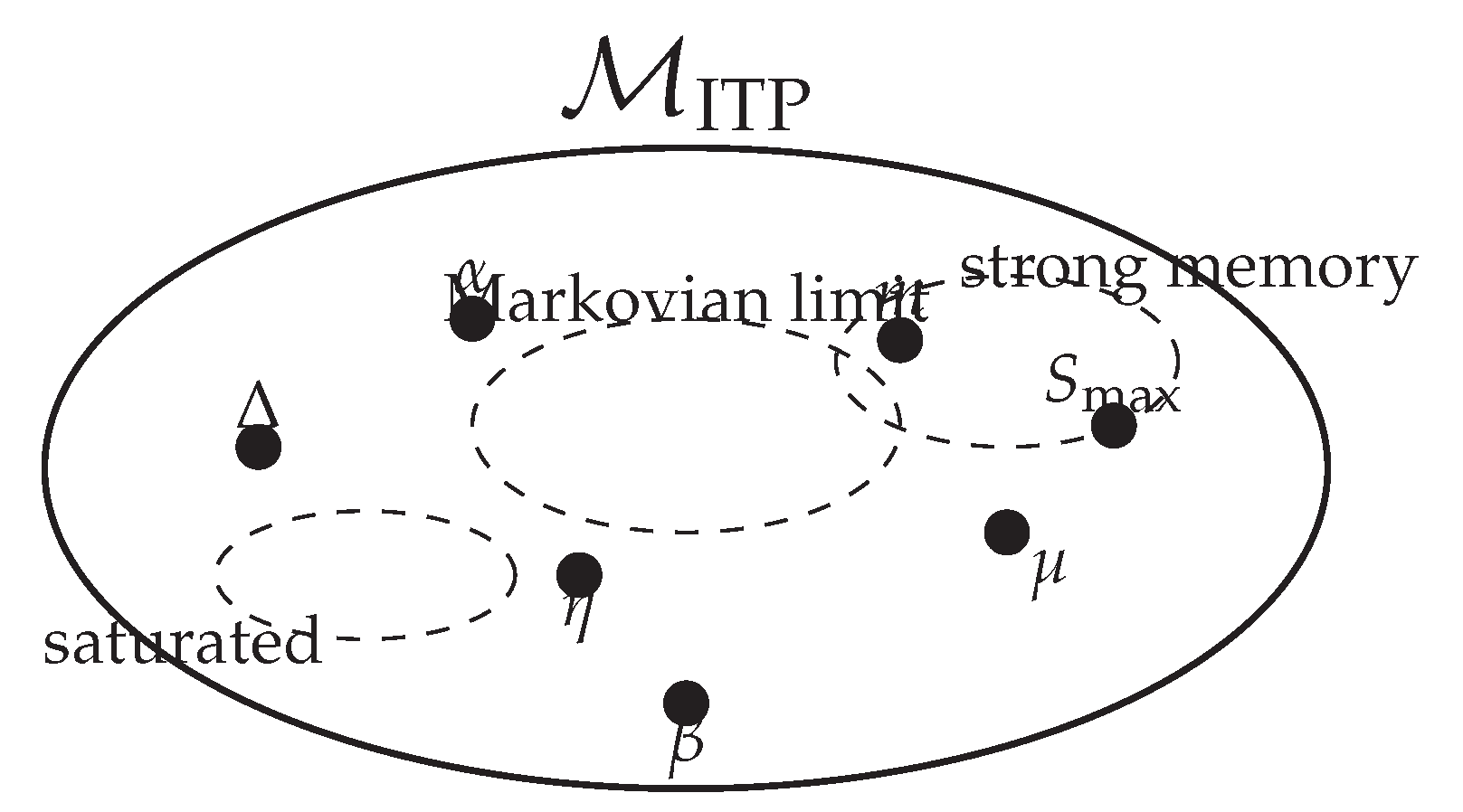
Figure 2.
Grid–based posterior proxy for the memory horizon inferred from the compilation under an exponential kernel. The curve is constructed from and normalized over the grid. The edge–seeking behaviour reflects insufficient constraining power rather than a sharp measurement of .
Figure 2.
Grid–based posterior proxy for the memory horizon inferred from the compilation under an exponential kernel. The curve is constructed from and normalized over the grid. The edge–seeking behaviour reflects insufficient constraining power rather than a sharp measurement of .
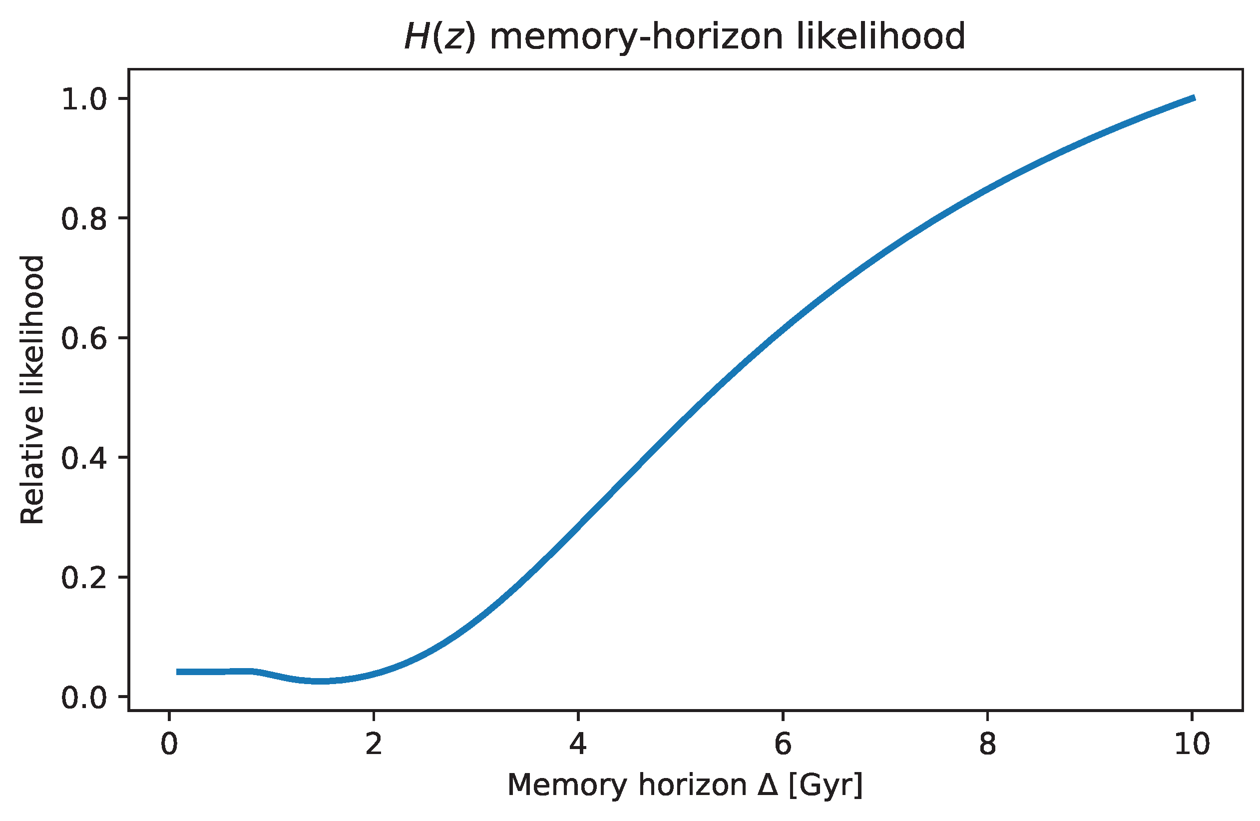
Figure 3.
Null test for the inference using shuffled residuals. Shuffling destroys any coherent redshift–ordered structure while preserving individual uncertainties. The distribution of best–fit scores across null trials is compared against the observed curve. In the present dataset, the observed behaviour is not exceptional relative to the null ensemble.
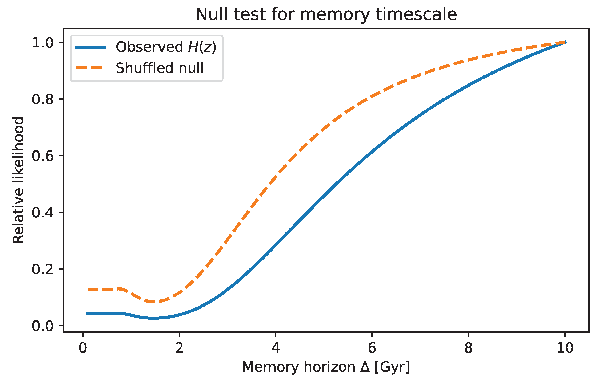
Table 2.
Illustrative posterior correlations in a five–parameter ITP cosmology fit. Values are indicative and quoted here to show structure, not as final measurements.
Table 2.
Illustrative posterior correlations in a five–parameter ITP cosmology fit. Values are indicative and quoted here to show structure, not as final measurements.
| Parameter pair | Correlation |
Disclaimer/Publisher’s Note: The statements, opinions and data contained in all publications are solely those of the individual author(s) and contributor(s) and not of MDPI and/or the editor(s). MDPI and/or the editor(s) disclaim responsibility for any injury to people or property resulting from any ideas, methods, instructions or products referred to in the content. |
© 2026 by the authors. Licensee MDPI, Basel, Switzerland. This article is an open access article distributed under the terms and conditions of the Creative Commons Attribution (CC BY) license (http://creativecommons.org/licenses/by/4.0/).
Copyright: This open access article is published under a Creative Commons CC BY 4.0 license, which permit the free download, distribution, and reuse, provided that the author and preprint are cited in any reuse.


