
Submitted:
27 January 2026
Posted:
27 January 2026
You are already at the latest version
Abstract
The search for life beyond Earth has traditionally relied on static habitability criteria, most prominently the presence of liquid water and suitable surface temperatures. These criteria are useful, but they ignore a deeper feature of planetary history: life does not simply fit into an environment, it emerges when a planet has developed enough internal coordination to support self-maintaining chemical networks. This work introduces the Ripeness Framework, a quantitative model that evaluates planetary life potential as a cumulative, time-integrated measure of coordination across five interacting factors: (i) cosmic inheritance, (ii) material substrate, (iii) geodynamic energy, (iv) feedback stability, and (v) external modulation. Two functionals are formulated: a linear ripeness functional and an enhanced CIOU functional that incorporates cross-domain coupling, information accumulation, and stability weighting, thereby encoding explicit non-Markovian path-dependence. Motivated by galaxy- and cosmology-scale results in which internal state and homeostatic memory dominate over instantaneous environment, ripeness is treated as an internal-state-first quantity: environment modulates and exposes ripeness but does not by itself create life. Toy simulations for Earth, Mars, and Europa reproduce three distinct developmental patterns: Earth shows non-linear acceleration in late-stage maturity, Mars exhibits developmental collapse, and Europa remains in a nascent pre-threshold state. A synthetic exoplanet ensemble with N = 106 planets demonstrates that classical habitable-zone metrics and developmental ripeness select systematically different targets: only a minority of planets are both environmentally “habitable” and developmentally ripe, while a larger population is developmentally ripe outside the classical habitable band. The framework yields falsifiable predictions: complex life should occur only on worlds that surpass a ripeness threshold and sustain cross-domain coupling over geological timescales; discovery of complex life on a low-ripeness world would falsify the CIOU-enhanced formulation. This approach reframes habitability from a spatial label to a developmental trajectory, and provides a testable basis for prioritising biosignature targets within a cyclic, non-Markovian cosmology. In other words, a planet may not be ripe for life in this time, but could ripen to develop and sustain life in the future.
Keywords:
ripeness equation
; planetary habitability
; origin of life
; abiogenesis
; exoplanets
; astrobiology
; cosmological memory
; Cyclic Infinite Organic Universe
1. Introduction
A central challenge in astrobiology is to understand the conditions under which life emerges. Classic habitability frameworks emphasise local constraints: surface temperature, liquid water, and circumstellar habitable zones [1,2]. These criteria are necessary, but they are incomplete. They describe conditions under which life could persist, but they do not explain why life emerges at particular times, why emergence appears structured across planetary histories, or why some worlds with apparently promising conditions never cross the line.
In standard planetary science and cosmology, abiogenesis is often treated as a stochastic chemical event driven by contingent interactions and accidents [3,4]. Earth’s record suggests a different picture: a prolonged maturation phase before robust biology became possible. Life did not appear at the first moment water and organics existed; it emerged after long-term stabilisation of energy flow, cycling, buffering, and self-regulation [5,6]. This motivates a developmental framing in which life is not only a function of present conditions, but of cumulative readiness.
That cumulative readiness is referred to here as ripeness. A planet ripens as it builds the internal structure required for stable, self-maintaining chemistry. Habitable zones remain relevant, but they are not causal engines. They are more like lighting in a room: good lighting does not write the book, it only makes the page readable.
Internal-state-first principle.
The core claim in this framework is:
Environment does not create life. It exposes ripeness.
External factors (stellar flux, impacts, orbital forcing, radiation environment) can trigger transitions, but only if the planet’s internal state has matured enough to respond by moving into a living regime. A planet can sit in a “nice” environment and remain unripe. Conversely, when ripeness is high, relatively modest modulation can make life not just possible, but difficult to avoid.
The aim of this paper is to give this internal-state-first view a quantitative form. The Ripeness Equation turns qualitative developmental intuition into a falsifiable metric that can be applied to Solar System worlds and synthetic exoplanet populations, and that fits naturally into a cyclic, non-Markovian cosmological framework.
2. The Ripeness Equation: Theoretical Formulation
2.1. Five Domains of Planetary Maturation
A planet’s developmental state is represented through five interacting domains, each mapped to a normalised readiness score in :
| Symbol | Domain (interpretation) |
| Cosmic inheritance (stellar composition, galactic environment, irradiation and volatile history) | |
| Material substrate (composition, atmosphere, hydrosphere, mineral diversity, surface–interior exchange) | |
| Geodynamic energy (heat flow, tectonics, chemical gradients, magnetic field) | |
| Feedback stability (climate regulation, buffering, resilience, relaxation times) | |
| External modulation (tides, cosmic rays, stellar neighbours, cluster/ISM context) |
The framework does not assign causal primacy to any single factor. It assumes that life emerges when these factors become sufficiently coordinated over time.
2.2. Ordinary (Linear) Ripeness Functional
Let denote system formation time. Define weights with for convenience. The ordinary ripeness functional is
This functional has three basic properties:
- Cumulative: history matters; ripeness is not a snapshot.
- Path-dependent: different developmental trajectories can reach the same .
- Sensitive to collapse: if key domains degrade (e.g. geodynamic shutdown), future accumulation can slow or stall.
2.3. Band-Limited Geodynamic Energy
Evidence from galaxy-scale homeostasis suggests that energy is a double-edged sword: it builds structure up to a point, then erodes memory and stability if excessive or poorly coupled. For planets, geodynamic energy is therefore treated as a band-limited contributor.
Let denote a raw geodynamic intensity measure (for example, surface heat flux or convective vigour). A readiness score is defined as
where f is small at very low , peaks at an optimal intermediate band, and decreases again when becomes large enough to destroy gradients and long-term structure. Simple choices include a bell-shaped curve or a piecewise linear approximation with a central plateau. The central assumption is that “more heat” is not always “better” for ripeness.
2.4. Life as a Threshold Transition
Ripeness is intended as a control functional for abiogenesis. A critical threshold is defined such that life becomes viable when ripeness crosses and sustains above that threshold:
The sustain time encodes the idea that a brief spike in readiness is not enough. The system must hold long enough for self-maintaining chemistry to lock in.
In the present toy simulations the sustain condition is approximated by requiring that the threshold is exceeded at the system age T. Explicit modelling of as an additional parameter is left for future work.
2.5. Internal State Versus Environment
To make the internal-state-first principle explicit, let denote a planet’s internal developmental state (gradients, cycling architecture, buffering, catalytic inventory), and let denote external modulation (irradiation, impacts, orbital forcing, etc.). The domain scores can be written as
while the internal state evolves with memory,
The present response therefore depends on the full developmental path. Environment can modulate and trigger, but the internal state decides whether any transition is sustained.
At galaxy scale, once mass and integrated history are controlled, residual dependences on environment are modest. The same logic is expected for planets: a world in the habitable zone with weak internal cycling and poor stability may never cross the ripeness threshold, while a world with deep internal structure can be tipped into a living state by modest external modulation. The environment provides the triggers; the internal state determines whether anything lasting happens.
2.6. CIOU-Enhanced Ripeness: Coupling, Memory, and Stability
The CIOU-enhanced functional upgrades Eq. (1) by rewarding sustained cross-domain coordination and penalising instability or collapse. A compact form is
where:
- weight pairwise synergy between domains.
- is a coupling map (simple choices include , or a correlation-like measure computed over a sliding time window).
- is an information/complexity accumulation rate proxy (for example, growth of chemical network diversity, cycling depth, or persistent disequilibrium capacity).
- downweights periods of collapse and rewards sustained regulation.
Formally, Eq. (6) is a Volterra-type functional: ripeness at time t depends on the entire prior trajectory , modulated by the stability weighting. In the language of the Cyclic Infinite Organic Universe (CIOU) framework, is a planetary-scale memory functional. It plays the same structural role for abiogenesis that non-Markovian kernels play for the cosmological background expansion: a retarded, path-dependent response that cannot be reduced to instantaneous state variables.
Simulation work on galaxy homeostasis indicates that the strongest internal coupling occurs between stability and memory: once mass is controlled, the correlation between these two variables is markedly stronger than any simple dependence on environment. This structure is mirrored at planetary scale by assigning larger to couplings between feedback stability () and memory-bearing domains ( and ). Ripeness is therefore not just “a lot” of each domain, but the emergence of a tightly bound stability–memory pair.
For concreteness, one can take
with an “instability” score (runaway greenhouse tendency, loss of atmosphere or ocean, magnetic collapse, repeated sterilisation events), and . increases when climate and geochemical feedbacks remain effective over multiple relaxation times, and decreases during episodes of regulatory failure.
At cosmological scale, previous non-Markovian fits to and within the CIOU framework indicate that the memory feeding the cosmic inheritance domain extends over several Hubble times rather than a short, effectively Markovian correlation time. Within the ripeness picture this means that is supplied by a long-range inheritance kernel, while – encode shorter planetary memories. thus sits naturally in a hierarchy of memory scales, from horizon-scale kernels down to local planetary development.
2.7. Abiogenesis Viewed Through the Ripeness Lens
Abiogenesis is treated here as a phase transition in an out-of-equilibrium reaction network. Ripeness acts as a control functional that shifts effective rates, connectivity, and robustness. Several standard criteria can be expressed in this language.
Network spectral threshold.
Let be an effective catalytic-production matrix for a coarse-grained chemical network. A necessary condition for self-amplifying organisation is that the spectral radius exceeds unity:
Ripeness increases by improving catalysts, gradients, transport, and stability. A simple toy representation is , or a distribution of K conditioned on planetary ripeness.
Percolation of catalytic connectivity.
Let be the probability that reactions are catalysed under ambient conditions. As ripeness grows, catalysts and surfaces become available and rises. Life-like global flux becomes plausible once
where is a percolation threshold for the network topology.
Nonlinear dynamics: emergence of a positive attractor.
In coarse kinetics, the trivial (dead) fixed point loses stability once an effective growth term becomes positive. Writing a toy replicator-metabolism variable ,
with noise , a living attractor becomes viable when
Here captures how ripeness shifts the system from a decay-dominated regime into one where self-maintaining growth is possible.
Thermodynamic power threshold.
Life requires sustained free-energy throughput above a minimum:
Ripeness increases effective coupling efficiency between energy sources and useful work by building the right cycling architecture and feedback loops.
These views are not competing pictures. They are different theoretical angles on the same transition, linked by the ripeness control functional.
3. Quantitative Implementation: Domains and Proxies
Each domain can be grounded in observable or model-inferred proxies (with subsequent normalization to ):
| Domain | Example proxies / measurement approaches |
| Cosmic inheritance | Stellar metallicity [Fe/H], stellar age, UV history, volatile delivery (from stellar spectra, galactic environment, dynamical models). |
| Material substrate | Atmospheric composition, ocean mass, mineral diversity, surface–interior exchange (from spectroscopy, interior models, Solar System analogues). |
| Geodynamic energy | Heat flux, presence or likelihood of plate tectonics, volcanic activity, magnetic dipole proxies (from thermal evolution and dynamo models). |
| Feedback stability | Climate relaxation time, buffering capacity, strength of negative feedbacks (from Earth-system modelling and palaeoclimate analogues). |
| External modulation | Cosmic ray environment, tidal forcing, encounters, cluster/ISM context (from galactic orbit reconstructions and stellar neighbourhood). |
The novelty lies not in the existence of these parameters, but in integrating them into a single developmental metric that is explicitly historical and falsifiable.
4. Methods
4.1. Monte Carlo Ripeness Bands for Solar System Worlds
To move beyond single fiducial values, Monte Carlo ensembles were constructed for Earth, Mars, and Europa. For each world, time was divided into geological epochs (for example, Hadean, Archean, Proterozoic, Phanerozoic for Earth). For each epoch and domain a fiducial readiness score was assigned based on qualitative assessments of each world’s history.
Uncertainty was represented by sampling
with truncation to , where encodes a fractional uncertainty in each domain and epoch. For each Monte Carlo realisation (here ) piecewise-constant trajectories were constructed and both the linear and CIOU ripeness functionals were evaluated at the present system age T,
A fiducial ripeness threshold was adopted and
was estimated for each of the three worlds.
All Solar System results reported here correspond to the run SOLAR_MC-20260115-035302 in the public ciou_ripeness_lab repository.1
4.2. Synthetic Exoplanet Ensemble
To illustrate how ripeness weighting reshapes target selection relative to classical habitability criteria, a synthetic exoplanet ensemble was constructed. N planets were generated orbiting main-sequence stars with stellar metallicities, ages, and incident fluxes () drawn from broad, empirically motivated ranges. For each planet the following were specified:
- a cosmic inheritance score as a function of stellar metallicity and age;
- a material substrate score based on a mapping from volatile inventory, atmospheric mass fraction, and core–mantle fraction;
- a geodynamic energy proxy derived from planet mass and age, mapped to a band-limited readiness score ;
- a feedback stability score that decreases in regimes prone to runaway greenhouse, prolonged snowball states, or rapid atmospheric escape;
- an external modulation score that penalises extremes in stellar activity and evolutionary stage.
All scores were normalised to using simple linear or quadratic mappings. For each synthetic planet, linear and CIOU-enhanced ripeness at the stellar age were evaluated using a common parameter set, yielding and .
For comparison to classical habitability, an environmental habitability score was defined as
with , so that identifies planets near the centre of the conventional circumstellar habitable zone.
The fiducial ensemble results correspond to the run EXO-ENSEMBLE-20260115-042913. A robustness test with a narrower environmental band () uses the configuration EXO-ENSEMBLE-20260115-054022.
5. Simulation-Based Evaluation
5.1. Solar System Monte Carlo: Mature Earth, Collapsed Mars, Nascent Europa
In the baseline setup with , the Monte Carlo ensembles yield
where means and standard deviations are estimated over realisations.
Figure 1 shows the probability density functions of for the three worlds. Earth is clearly separated from Mars and Europa in ripeness space.
Table 1 summarises the mean ripeness values for the three worlds.
In this implementation Earth is mature, Mars is marginal and collapsed, and Europa is nascent: the three worlds occupy distinct positions along the ripeness trajectory.
5.2. Expanded Developmental Classificati.on
A key advantage of is that it separates worlds with superficially similar present conditions by developmental direction. Extending beyond Earth, Mars, and Europa, additional worlds can be qualitatively classified under the ordinary versus CIOU framing, as summarised in Table 2.
These labels are working hypotheses. They indicate different positions and directions along the ripeness trajectory rather than final verdicts.
5.3. Synthetic Exoplanet Ensemble: Ripeness vs Classical Habitability
In the fiducial run with , only about of planets have environmental scores , whereas exceed the ripeness threshold . The overlaps are asymmetric: of planets are both high-H and high-ripeness, are high-H but sub-threshold (“pretty but unripe”), and are low-H but super-threshold (“unpretty but mature”). In this toy ensemble, more than twice as many planets are developmentally mature outside the classical habitable band as there are planets that are both habitable-looking and ripe.
Figure 2 compares the environmental score H to for a representative subsample of the ensemble. Classical habitable-zone candidates (high H) do not always achieve high ripeness, and many high-ripeness planets live at only moderate H. Developmental ripeness and instantaneous environment are therefore distinct axes of selection. Ranking planets by rather than H reorders the target list: the most promising biosignature targets are those where internal state and stability have had time to develop, not necessarily those sitting in the centre of the habitable zone at the present epoch.
5.4. Robustness to the Width of the Habitable Band
The environmental score H is intentionally simple: a Gaussian weight around Earth-like flux with width . One might worry that the mismatch between classical habitability and ripeness is an artefact of the particular choice . To check this, the ensemble was repeated with a narrower band, , keeping all other assumptions fixed.
As expected, narrowing the band reduces the overall fraction of high-H planets but leaves the joint structure intact. For , only of planets satisfy , while the fraction with remains . The overlaps remain strongly asymmetric: of planets are both high-H and high-ripeness, are high-H but sub-threshold, and are low-H but super-threshold. Tightening the flux-based habitability criterion therefore amplifies the “unpretty but mature” population.
The central conclusion is thus insensitive to reasonable choices of : developmental ripeness and instantaneous environmental comfort are structurally distinct axes. Changing rescales the number of classical habitable-zone candidates but does not remove—and in this case strengthens—the population of developmentally ripe planets outside the traditional habitable band.
6. Discussion: Ripeness, Internal State, and a Cyclic Non-Markovian Universe
The simulations presented here are deliberately simple, but they already enforce a clear distinction between two stories about life: one in which environment is primary, and one in which internal state is primary.
In the Solar System Monte Carlo, Earth emerges as a narrowly super-threshold world () with , while Mars and Europa remain robustly sub-threshold. This is not because their present environments are uniformly hostile. Early Mars likely had liquid water, and Europa hosts a long-lived ocean. The difference lies in their developmental trajectories: they do not sustain cross-domain coordination over time. Under the Ripeness Framework, the emergence of life is not a question of whether a world ever passes through a “nice” environmental state; it is a question of whether internal organisation, energy flow, and feedback stability integrate long enough to cross a cumulative threshold.
The synthetic exoplanet ensemble makes the same point at scale. Only a minority of planets are both environmentally favoured (high H) and developmentally ripe (high ), while a larger population is developmentally ripe outside the classical habitable band. The “pretty but unripe” and “unpretty but mature” quadrants are not small corrections; they dominate the structure of the joint plane.
This internal-state-first structure is consistent with the Cyclic Infinite Organic Universe (CIOU) model. In galaxy and cosmic-web analyses, internal structure and mass history dominate over instantaneous environment: once mass is controlled, environment behaves as a modulator of outcomes rather than a primary cause. The ripeness simulations show the same logic at planetary scale. A planet’s present snapshot—position in a habitable zone, current temperature, current flux—is not enough. What matters is the integrated internal history: how much energy has flowed through, how tightly feedback loops have locked in, how often stability has been broken and rebuilt.
Within this picture, planets are local organs of a larger organism. Ripeness is a scalar summary of their local developmental state along the organism’s cycle. The CIOU-enhanced functional makes this explicit by including cross-domain couplings, information accumulation, and stability weighting. is not simply a sum of present-day scores; it is a memory functional over the planet’s path. That memory is what distinguishes Earth from Mars and Europa in the Monte Carlo, and what populates the “unpretty but mature” quadrant in the exoplanet ensemble.
The broader CIOU programme now displays a hierarchy of memory. Horizon-scale fits to and require a long-range cosmological kernel acting on the background expansion. Galaxy-scale analyses of virialisation in simulations reveal short, negative Gyr-scale kernels in which nonlinear structure behaves as an effective viscosity on local expansion. The ripeness functional sits one rung down again, as a planetary memory functional summarising the integrated history of cycling, stability, and substrate. Planets, galaxies, and the background thus realise the same non-Markovian logic at different scales.
The framework is also falsifiable. If future observations uncover complex, ecosystem-scale life on a world that scores as low-ripeness under any reasonable choice of domain proxies and weights (a Mars-, Europa-, or Enceladus-like world in this scheme), then the CIOU-enhanced ripeness functional is wrong or incomplete. Conversely, a pattern in which robust biosignatures are preferentially detected on planets that would score high in —worlds with long-lived gradients, persistent geodynamic cycling, and strong feedback stability—would support the view that life is a phase transition in a maturing system rather than an isolated lucky event.
The present implementation is intentionally minimal, with approximate domain mappings and toy ensembles. The core claim is not that the particular numbers are final, but that the structure of the Ripeness Equation is a useful way to pose the question. In a cyclic, non-Markovian universe with memory, the emergence of life is a property of trajectories, not snapshots. The environment does not start the story; it reveals when the story is ready to move.
7. Predictions and Falsification
7.1. Hard Falsifier
If complex or multicellular life is confirmed on a world that robustly scores low under (for example, Europa, Enceladus, or present-day Mars under conservative stability penalties), then the CIOU-enhanced ripeness formulation is falsified. The linear could in principle survive as a weaker statement, but the non-Markovian stability-weighted version would be ruled out.
7.2. Validation Direction
Worlds with high should be the first to show ecosystem-scale biosignatures (persistent chemical disequilibrium, coupled atmospheric signatures) in survey order. This is not because such worlds are observationally favoured, but because development makes them dynamically loud.
7.3. Internal-State-First Forecast
If two planets share similar present-day habitability conditions, the one with stronger inferred developmental history (long-lived gradients, cycling, buffering, and stability) should be more likely to show biosignatures. In short: the environment is the stage, not the playwright.
8. Limitations and Future Work
Several limitations are clear. The domain proxies are deliberately schematic; real exoplanet catalogues will require more careful mappings from observables to . The threshold is currently a modelling choice rather than an inferred quantity, and the domain weights and couplings have not yet been constrained by data. The present work is therefore best viewed as a scaffold: a first quantitative expression of the idea that life emerges when ripeness silently crosses a line.
Empirical grounding.
Current ripeness values rely on proxies and model inference. Strong validation requires improved constraints on volatile inventories, thermal states, atmospheric cycling, and long-baseline stability indicators for exoplanets.
Determining .
The critical threshold is hypothesised, not known. Estimating it will require connecting planetary-scale stability measures to laboratory and theoretical thresholds for network emergence (spectral, percolation, kinetic, and thermodynamic criteria).
Domain weights and couplings.
For demonstration, weights can be taken as equal and coupling terms simple. Ultimately, , , and stability parameters should be inferred (for example, via Bayesian calibration) as multi-world datasets improve. In principle, the domain weights and couplings could be constrained by planetary ensembles in the same spirit that homeostatic observables have been calibrated in galaxy simulations and surveys.
Exoplanet data limitations.
Many proxies are currently only weakly observable for exoplanets. The framework is designed to scale with better data rather than assume that the necessary measurements already exist.
Degeneracy and multiple pathways.
Different developmental routes can reach similar ripeness. This is a feature: it allows multiple viable biochemical pathways, while still requiring sustained coupling and stability. The aim is not to force a single origin story, but to unify them under a common developmental metric.
Future work can connect ripeness estimates directly to observational strategies for upcoming missions, link the planetary functional more tightly to the cosmological memory kernels that feed , and explore whether ripeness can be inferred statistically from ensemble patterns in exoplanet populations.
9. Conclusions
The Ripeness Equation reframes habitability as a developmental trajectory rather than a static label. The ordinary functional captures cumulative readiness; the CIOU-enhanced functional encodes cross-domain coupling, stability, and non-Markovian memory. Together they yield a direct claim: life emerges when a planet becomes ripe enough that self-maintaining chemistry is no longer a lucky accident but a phase transition made likely by cumulative coordination.
Within the broader CIOU picture, this is one expression of a cyclic, non-Markovian universe in which internal state and memory dominate dynamics across scales. Galaxies, stars, and planets are different rungs of the same ladder; ripeness is how that ladder feels inside a world.
The cleanest takeaway is also the bluntest:
The environment does not start the story. It reveals that the story is ready to move.
Data Availability Statement
All MCMC runs and relevant scripts and data can be found at https://github.com/Atalebe/ciou_ripeness_lab
References
- Kasting, J.F.; Whitmire, D.P.; Reynolds, R.T. Habitable Zones around Main Sequence Stars. Icarus 1993, 101, 108–128.
- Kopparapu, R.K.; Ramirez, R.; Kasting, J.F.; et al. Habitable Zones around Main-Sequence Stars: New Estimates. Astrophysical Journal 2013, 765, 131.
- Ruiz-Mirazo, K.; Briones, C.; de la Escosura, A. Prebiotic Systems Chemistry: New Perspectives. Chemical Reviews 2014, 114, 285–366.
- Szostak, J.W. The Narrow Road to the Deep Past: In Search of the Chemistry of the Origin of Life. Angewandte Chemie International Edition 2017, 56, 11037–11043.
- Sleep, N.H. Geological and Geochemical Constraints on the Origin and Evolution of Life 2018. General reference to the maturation timescale perspective.
- Foley, B.J.; Driscoll, P.E. Whole Planet Coupling between Climate, Mantle, and Core. Geochemistry, Geophysics, Geosystems 2016, 17, 1885–1914.
| 1 | The repository contains the exact configuration files and scripts used to generate Figure 1. |
Figure 1.
Monte Carlo distributions of CIOU ripeness for Earth, Mars, and Europa. Each histogram shows the probability density of from realisations per world. Earth is narrowly super-threshold with mean , while Mars () and Europa () remain robustly sub-threshold under the chosen parameters.
Figure 1.
Monte Carlo distributions of CIOU ripeness for Earth, Mars, and Europa. Each histogram shows the probability density of from realisations per world. Earth is narrowly super-threshold with mean , while Mars () and Europa () remain robustly sub-threshold under the chosen parameters.
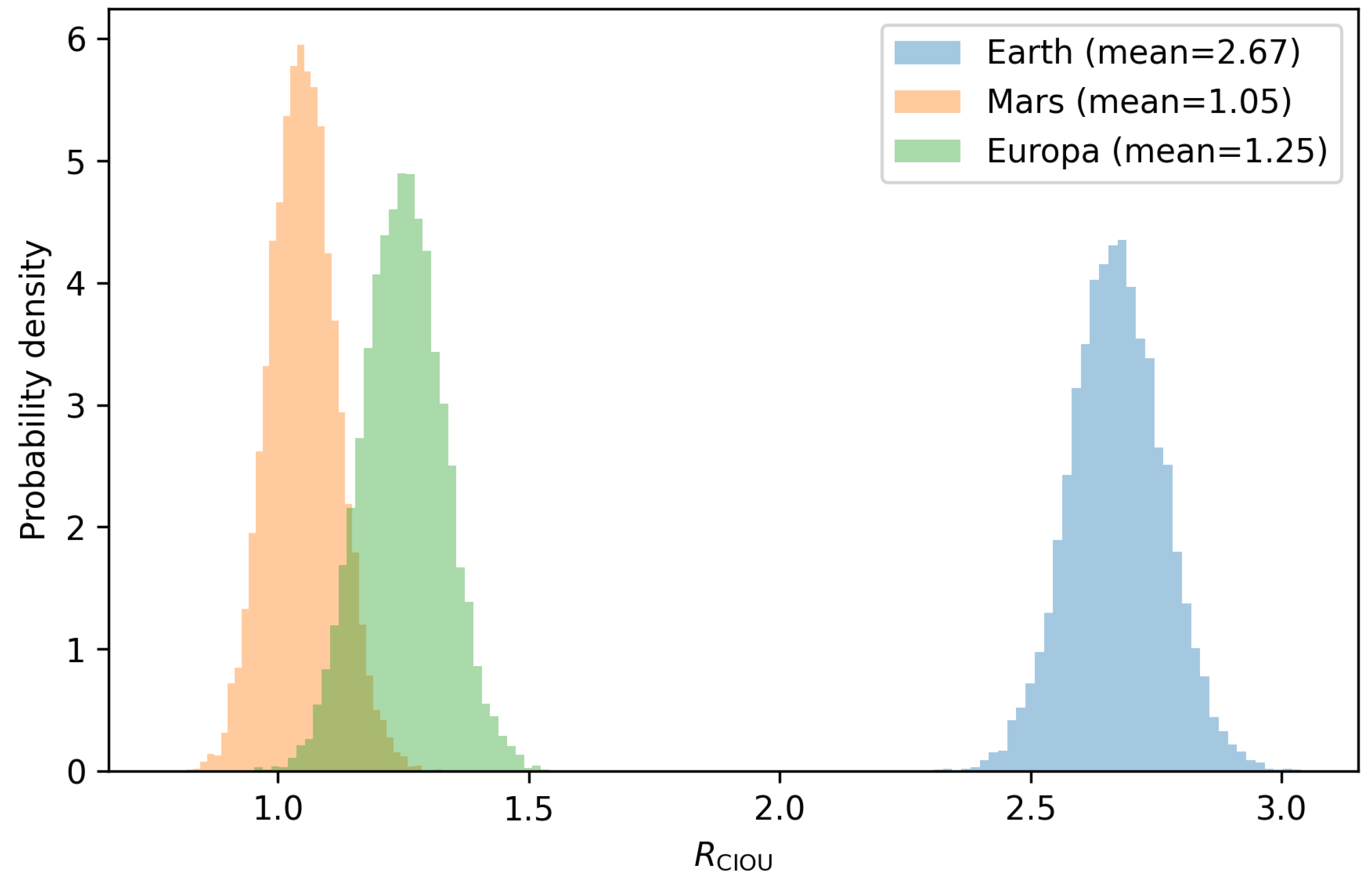
Figure 2.
Environmental score H versus CIOU ripeness for a subsample of the synthetic exoplanets. Classical habitable-zone candidates (high H) do not always achieve high ripeness, and many high-ripeness planets live at only moderate H.
Figure 2.
Environmental score H versus CIOU ripeness for a subsample of the synthetic exoplanets. Classical habitable-zone candidates (high H) do not always achieve high ripeness, and many high-ripeness planets live at only moderate H.
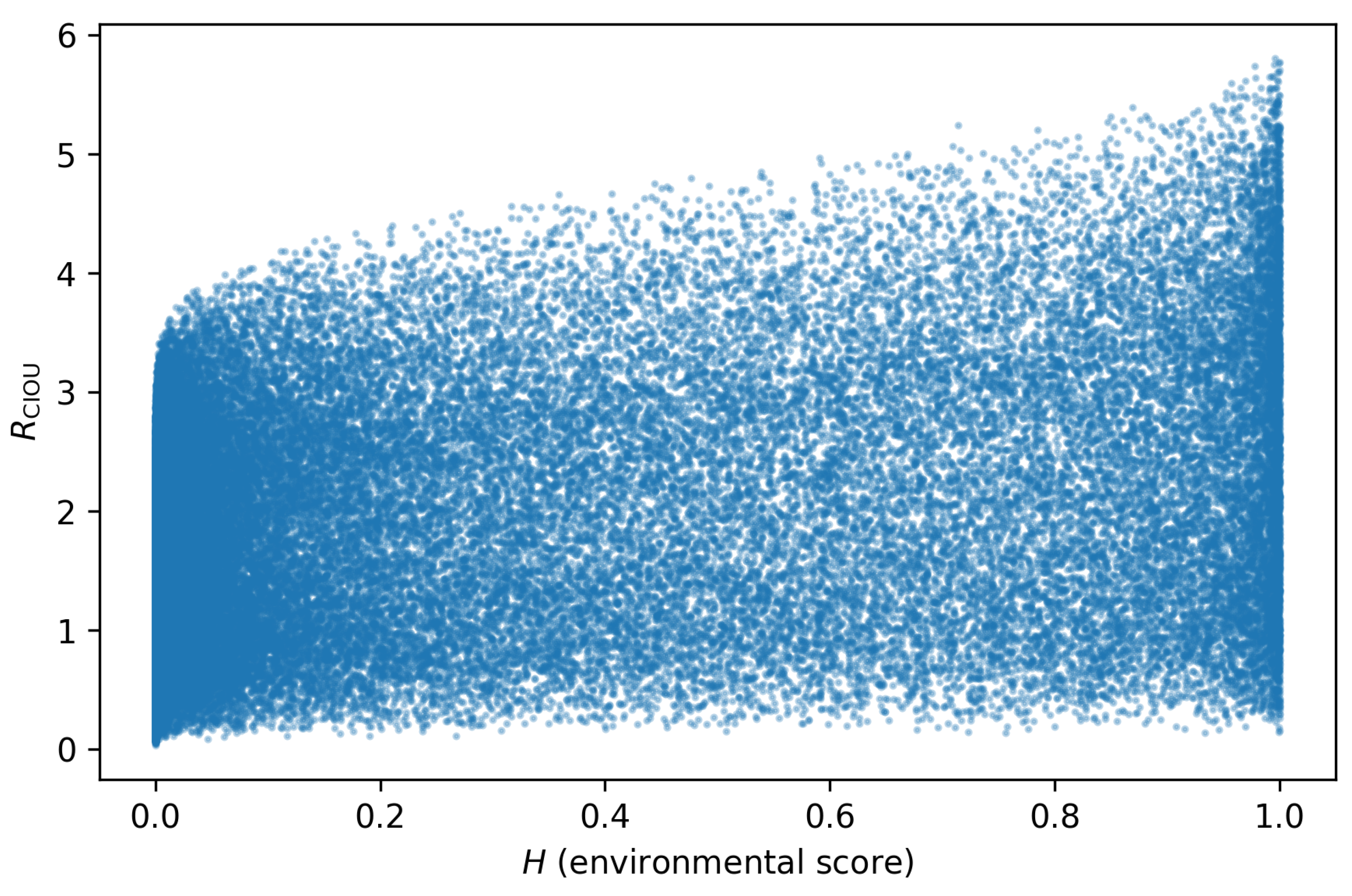

Table 1.
Summary of Monte Carlo ripeness statistics for Earth, Mars, and Europa (means over realisations).
Table 1.
Summary of Monte Carlo ripeness statistics for Earth, Mars, and Europa (means over realisations).
| World | Interpretation | ||
| Earth | 2.31 | 2.67 | Mature; crossed and sustained the complexity threshold. |
| Mars | 1.41 | 1.05 | Collapsed; early promise reversed by loss of regulation. |
| Europa | 1.38 | 1.25 | Nascent; constrained by integration time and exchange pathways. |
Table 2.
Qualitative classification of additional worlds under the ordinary vs CIOU framing.
| World | Ordinary ripeness | CIOU ripeness | Developmental classification |
| Earth | High | Very High | Mature: sustained coupling and threshold crossing. |
| Mars | Moderate | Low | Collapsed: early promise reversed by geodynamic failure. |
| Europa | Low | Very Low | Nascent: constrained by time and exchange pathways. |
| Venus | Moderate | Extremely Low | Aborted: feedback collapse and irreversible instability. |
| Enceladus | Moderate | Low | Ephemeral: transient engine, insufficient stability window. |
| Titan | High | Moderate | Divergent pathway: development under non-water chemistry; coupling uncertain. |
| TRAPPIST-1e | Model-dependent | Stability-dependent | Stability-limited: outcome set by atmospheric–climate regulation. |
Disclaimer/Publisher’s Note: The statements, opinions and data contained in all publications are solely those of the individual author(s) and contributor(s) and not of MDPI and/or the editor(s). MDPI and/or the editor(s) disclaim responsibility for any injury to people or property resulting from any ideas, methods, instructions or products referred to in the content. |
© 2026 by the authors. Licensee MDPI, Basel, Switzerland. This article is an open access article distributed under the terms and conditions of the Creative Commons Attribution (CC BY) license (http://creativecommons.org/licenses/by/4.0/).
Copyright: This open access article is published under a Creative Commons CC BY 4.0 license, which permit the free download, distribution, and reuse, provided that the author and preprint are cited in any reuse.


