
Submitted:
26 January 2026
Posted:
26 January 2026
You are already at the latest version
Abstract
As global aquaculture continues to expand there is an increasing interest for sustainable and non-invasive tools to monitor fish growth. Nile tilapia (Oreochromis niloticus) is one of the most farmed species worldwide. Its biomass estimation often relies on manual sampling or stereo-cameras systems limited by water turbidity. This study establishes a robust relationship between lateral Target Strength (TS) and the total length (TL) and weight (W) of Nile tilapia using a cost-effective 201 kHz single-beam echosounder. Measurements were conducted with free-swimming fish in a controlled pond environment (TL range 13–44 cm). The results show a strong linear correlation between acoustic and biometric data. Specifically, the relationship for mean TS was defined as TSmean = 20.1log(TL) − 66.7 (R2=0.91) and TSmean = 6.3log(W) − 55.4 (R2=0.96), proving the system’s accuracy for biomass estimation. Furthermore, the Method of Fundamental Solutions (MFS) was employed for numerical validation based on X-ray morphometry of the swim bladder. A very good agreement was observed between experimental data and numerical simulations, reinforcing the validity of the acoustic models despite the inherent complexity of biological targets. These findings demonstrate that calibrated single-beam acoustic systems provide a viable, non-intrusive tool for real-time monitoring in aquaculture ponds.
Keywords:
Nile tilapia
; target strength
; single-beam echosounder
; aquaculture monitoring
; numerical methods
; blue economy
1. Introduction
Aquaculture production reached a record 130.9 million tons in 2022, with a total value of 295.7 billion dollars [1]. Nile tilapia (Oreochromis niloticus) is the fourth most farmed species, with a global production of 5.3 million tons in the same year. As fishery resources continue to decline due to overfishing, pollution, poor management, and other factors, aquaculture is expected to expand to meet the growing demand for food. However, this growth must be achieved sustainably, ensuring ecosystem protection, pollution reduction, biodiversity conservation, and social equity. The concept of Blue Transformation, an international initiative, presents key challenges for fisheries and aquaculture. Within this framework, the expansion of aquaculture aims to be both sustainable and resilient, addressing environmental and social concerns while enhancing global food security [1]. Nile tilapia aquaculture can be developed in cages, ponds, or tanks. This species exhibits rapid growth, with individuals increasing their weight by approximately 50% within 6 to 9 months, making it well-suited for farming. To ensure adequate growth, it is essential to monitor various parameters, such as size, weight, and population density. For this reason, regular sampling must be carried out. Traditionally, aquaculture production in cages or tanks has been monitored through manual sampling, performed either by farm staff or machinery. However, this method is often invasive to fish. In recent years, video-based systems have been increasingly used to estimate fish length and monitor various procedures in aquaculture. These non-intrusive systems can be mono, stereo, or drone-based, and their data can be processed automatically, often incorporating artificial intelligence [2,3,4]. However, video systems are limited by factors such as water depth and turbidity. Alternatively, underwater acoustics has been employed to estimate biomass in free water [5]. An increasing number of studies focus on the application of acoustic techniques for monitoring fish growth in cages and tanks [6,7,8,9]. In these studies, a relationship between target strength (TS) and fish length was found from different perspectives (ventral and lateral). TS is defined as the acoustic energy backscattered by an individual fish [5]. The TS returned by a fish depends on several factors, with some of the most important being fish size, the presence or absence of a swim bladder, and swimming orientation. Liu et al. (2022) [10] demonstrated that a reliable relationship between target strength (TS) and fish length can be obtained for Nile tilapia using a scientific echosounder. In their study, Nile tilapia of different sizes were anchored and measured in a laboratory tank. Scientific echosounders are commonly used, as they can compensate for TS variations based on the fish’s position within the acoustic beam. Moreover, they provide valuable information about fish swimming trajectories. However, their high cost limits their widespread use as a monitoring tool in aquaculture. On the other hand, Dwinovantyo et al. (2023) [11] used a single-beam scientific echosounder (Simrad EK15) and a fish finder (Furuno FCV-628) to establish a relationship between Nile tilapia length and TS in a tank. To achieve this, the fish were anchored to obtain TS-length data. In this study, a strong relationship between TS and the total length of Nile tilapia was found. During the measurements, the fish were swimming freely, making the conditions similar to those in production environments. A single-beam echosounder was used, which, although calibrated, is a cost-effective system when compared to scientific echosounders. Preliminary results were described in [12,13]. Because of this, it has the potential to become a useful non-invasive tool in tilapia aquaculture. Its adoption could help producers align with the Blue Transformation guidelines.
2. Materials and Methods
2.1. Biometric Data Collection
The data were collected at Centro de Investigación Piscícola (CIMPIS) of the Universidad Agraria La Molina (Lima, Perú) (12°05’03" S - 76°56´44.8"W) from December 2018 to December 2019. To do it, a pond of 4.0 x 4.0 x 1.5 m was built. Nile tilapia (Oreochromis niloticus) with total length (TL) between 13 and 44 cm were selected and divided into 8 groups. The maximum size dispersion for each group was 2.0 cm, with an uncertainty of ±0.5 cm. The number of fish in each group varied between 6 and 20 fish depending on the availability. A description of selected groups is shown in Table 1. To obtain TL of each fish, an ichthyometer (INC Aquatic Eco-Systems) was used. The fish weight (W) was obtained (Figure 1) using a digital precision scale Bondibuy SF-400 (±1g). Morphological data acquisition process is described in [14].
2.2. Acoustic Data Collection
Acoustic measurements were performed using a Biosonics DT-X echosounder working with a 201 kHz single beam transducer. The transducer was placed at the end of the pond such the acoustic beam was parallel to the water surface. Thus, lateral point of view of the fish was recorded (Figure 2). Acoustic data were collected during 2 to 5 days for each length group shown in Table 1. During the measurements, fish were swimming freely into the pond. Echosounder measurement settings are presented in Table 2. Data were recorded using Visual Acquisition software from Biosonics®. For ease the analysis, short files were recorded, with maximum duration of 30 minutes.
2.3. Acoustic Data Analysis
Acoustic data were collected and analysed using Sonar 5-Pro [15]. Echograms were transformed and a threshold of 95 dB was used to obtain higher quality images. Due to a single beam transducer was used, 2D Single Echo Detector (SED) algorithm was applied. Traces were isolated manually, and they be ranked in terms of quality. To do it, TS profile of each trace was analysed. If the trace had the typical “v” shape, it was stored otherwise it was rejected. Two examples of selected traces are shown in Figure 3. For each trace maximum TS, mean TS and distance from the centre of gravity of the trace were calculated. When de distance from the centre of gravity was lower than 1 meter, traces were discarded. Data obtained from Sonar5-Pro were transferred to Statgraphics Centurion XIX software for statistical analysis. Mean and maximum TS versus fish length relationships were obtained. The linearized equation (1) was used
where a is the slope and b is the intercept and TL is expressed in centimetres. In fisheries, a fixed slope a=20 has been extensively used [16]. Nevertheless, McClatchie et al., 2003 [17] shown that, when information related to a wide range of fish size is available,a free slope provides better TS vs TL fits. In this study both, a and b, were obtained from lateral TS measurements and fish sampling for each group.
2.4. Numerical Simulations of TS from Nile Tilapia
For the numerical estimation of TS, the Method of Fundamental Solutions (MFS) was selected. MFS is a non-mesh simulation method based on reproducing the field through a linear combination of a set of virtual sources located outside the domain of interest [18]. A determinant advantage of the MFS is its capability to evaluate the acoustic backscattered field at any working distance between the fish and the echosounder, but, being a meshless method, avoiding the high computational costs associated with the use of other numerical methods with a mesh, as it is the case of boundary element method or finite element method [19]. The propagation of sound within a homogeneous acoustic space can be described mathematically in the frequency domain by using the Helmholtz differential equation (2):
where
in the case of 3D problem, p[Pa] is the acoustic pressure, the wave number, the angular frequency, f[Hz] the frequency and c [m/s] the sound propagation velocity within the acoustic medium. For the 3D case, assuming a point source placed within the propagation domain, at point with coordinates () [m], it is possible to establish fundamental solution G, for the sound pressure, and H, for the particle velocity [m/s], at a point with coordinates x [m], which can be written respectively as:
In these equations, r [m] corresponds to the distance between the source point and the domain point given; represents the direction along which the particle velocity is calculated and [kg/m3] the medium density. Being the swimbladder responsible for the most significant contribution of the acoustic dispersion [20], the Nile tilapia TS was evaluated considering the acoustic backscattering from the swimbladder. A characterization of the swimbladder of the species was conducted during the experiment extracting individuals from the same tanks used in the acoustic measurements. A set of 25 individuals were x-ray scanned to obtain the morphometry of the swimbladder and flesh. The aim was to obtain the allometric relations relating to the swimbladder length and the total fish length, which allow to develop geometrical models for TS estimation. From the X-Ray set, 6 individuals were selected, by visual inspection ,to develop the swimbladder model shape. The procedure was as following: for each individual, two orthogonal 2D images of the inflated swimbladder were extracted, which allows to reconstruct a 3D swimbladder model. The 2D images were processed by using our own developed code and the Image Processing App in Matlab®. The masks for the fish flesh and swimbladder were extracted, smoothed and processed to characterize the best elliptic fit for both xy and and xz planes, being x defined as the fish axis direction. The two orthogonal 2D ellipses were combined for constructing the best 3D prolate ellipsoid for modelling the swimbladder. This process (Figure 4) was conducted for every fish and considered to perform the numerical estimations. The individuals were preserved in ice and scanned immediately after being extracted from the tank. The size distribution was selected to be distributed along the size range of the experiment.
The swimbladder was modeled as a volume with pressure release on its surface [21]. The properties considered for the materials were: [m/s], [kg/m3], [m/s] and [kg/m3]. The TS was calculated at 3 meters, as was the working length in the experimental tanks. Figure 4 (right) shows the distribution of the boundary points and the virtual sources used in the MFS calculation. To consider the role of the fish orientation, the directivity of the TS was evaluated by rotating the angle between the fish axis and the beam incidence direction degree by degree from -corresponding to incidence from Head to Tail (H2T) orientation- to -meaning Tail to Head (T2H) orientation-, being the orientation corresponding to the lateral insonification of the fish [9] In the absence of more accurate information about the swimming orientation distribution of the fish in the tank, to compare with the experimental measurements, we consider a gaussian orientation distribution [22] centered at (lateral insonification) amd . To reproduce the realistic experimental situation, the emitter transducer was modeled as a flat piston for the operating frequency of 201 kHz, with a beam angle of at -3 dB.
3. Results
3.1. Experimental Results
Results obtained are presented in Table 3. For each group, the number of manually isolated good quality traces was between 1402 and 8696. The lower number corresponded to the group with smallest size (14.1 cm). However, the largest number of traces come from group 3 with mean TL of 21.5 cm. A mean TS distribution was obtained per group and average value; median and standard deviation were obtained from that. The same applies to maximum TS distribution for each group (Table 3). For TSmean case, average values from -42.2 to -34.8 dB were observed. Average values ranged from -41.0 to -32.0 for TSmax. Figure 5 shows the violin plots for each TS distribution. On the top, for maximum TS, TSmax, and on the bottom for mean TS. For both, higher length involves higher TS as expected indicating the direct relationship between TL and TS, TSmean. The linear regression fits of average values of TS (mean and maximum) versus TL are also presented in Figure 5, including the results extracted both from experimental measurements and numerical estimations.
Two empirical equations (6),(7) were obtained for relating the Nile tilapia length with the measured TS at 200 kHz for TSmean and TSmax. In both cases, a good linear correlation was obtained, with R2 higher than 0.9, bring higher for the TSmax.
Different studies have shown that there is a direct relationship between length and weight of the Nile tilapia [14,23,24]. That means that from measured TS, weight of Nile tilapia could be estimated. For this reason, mean weight presented in Table 1 and average values of Tmean and TSmax were fitted to the Total Length. The regression equations obtained are shown below (equations 4 and 5). High R2 correlation coefficients were achieved, R2=0.96 for W-TSmean and R2=0.9 for W-TSmax relationship. That fact implies that using those equations (6)–(9) total length or weight could be converted to TS, and vice versa, in a robust way.
3.2. Numerical Simulations of Nile Tilapia Target Strength
Numerical estimates were performed for the range of sizes observed in the tank. The geometric model was developed from the X-ray images, obtaining a relationship between the swimbladder geometrical properties and fish length. Considering the allometry reported for the external morphology of Nile tilapia [14] and for the swimbladder in various species [25], the length (SBL) and volume (SBV) of the swimbladder were related to the total length of the fish according to a functional power relationship. The results of the analysis are illustrated in Figure 6, while the values obtained for the fit parameters are given in Table 4.
To evaluate the influence of the swimbladder dimension on the TS, focusing on TS-log(TS) relationship, its maximum lateral cross section (SBCS). Figure 7 shows the relationship between the maximum lateral effective section and the total length of the fish.
It should be noted that the exponent of this potential relationship, SBCS, is related to the slope of the TS-log(L) relationship (McClatchie et al., 2003). Because the gas-filled swimbladder accounts for about 90–95% of the backscattering cross-section in swim bladdered fishes, if the TS is effectively governed by the swim bladder’s effective acoustic cross-section, it would be expected that this slope, both from the numerical estimations and experimental measurements, to be close to, but not higher than, 10 b, being b=2.62 (2.39,2.86) (Table 4).
The numerical model considered six sizes distributed along the experimental size range. Based on the best elliptical fits of the swim bladder masks in the two orthogonal planes, the corresponding three-dimensional geometry was constructed. To account for the variation in the swimming direction of the fish, the directivity of the backscattered acoustic wave was evaluated. Figure 8 shows the TS values for different relative orientations between the fish’s axis and the direction of propagation of the acoustic beam for a swim bladder corresponding to an individual of TL=27 cm.
In order to compare with the experimental data, a Gaussian swimming distribution centered at (fish axis perpendicular to the direction of propagation) with a standard deviation of is considered. The numerical estimation is carried out for six TL values distributed along the measurement range based on the x-ray images. A linear relationship is obtained for both TSmax and TSmeanwith respect to log(TL). The results of these fits are (10),(11):
Figure 5 shows the comparison between the experimental data and the numerical predictions of the simplified models that consider swim bladder within a prolate spheroid shape.
4. Discussion
The results of this study establish a direct relationship between Target Strength (TS) and the total length (TL) of Nile tilapia (Oreochromis niloticus). The empirical equations derived for both TSmean and TSmean exhibit high correlation coefficients (R2 >0.9), validating the use of acoustic systems to monitor growth in aquaculture. Furthermore, the robust correlation found between TS and weight (W)-with R2 values reaching 0.96- suggests that biomass can be estimated through acoustic methods, facilitating real-time non-invasive production management. This acoustic approach presents some advantages over video-based systems that are typically used for fish sizing in aquaculture. Video systems are limited by water depth and turbidity, which often hinder visibility in ponds. In contrast, underwater acoustics can estimate biomass and size in turbid waters and across larger working distances, providing a complementary tool for various farm layouts. The morphology of the swim bladder was confirmed as the dominant factor in these acoustic measurements. Numerical simulations using the Method of Fundamental Solutions (MFS) indicated that the gas-filled swim bladder accounts for 90–95% of the backscattering cross-section [20]. Allometric analysis of X-ray images revealed that the maximum lateral cross-section of the swim bladder (SBCS) follows a power relationship: SBCS. As noted by McClatchie et al. [17], the slope of the TS vs. log(TL) relationship is closely tied to this exponent (b); if TS is governed by the SBCS, the slope would be expected to approach (approximately 26.2 in this case). There is a very good agreement between the experimental results and the numerical predictions generated by the Method of Fundamental Solutions (MFS). This correspondence confirms that the numerical model incorporates a Gaussian swimming distribution centered at a lateral aspect () to capture the influence of the behavior of the fish. While the numerical model predicted values that were consistently slightly higher than the experimental ones, this discrepancy is justified by the fact that the numerical model uses an idealized pressure-release surface for the swim bladder and assumes a perfectly controlled environment [17,21,22]. In the experimental pond, factors such as the acoustic damping from fish flesh, natural variations in swimming tilt, and the biological complexity of free-swimming fish inevitably lead to slightly lower TS values compared to the theoretical maximums of a prolate spheroid model. In a real-world fish farm, these results could be applied by installing fixed or mobile single-beam transducers to monitor growth rates without the need for manual sampling. Being the fish measured while swimming freely - unlike previous studies where fish were anchored - the resulting equations could be applicable to commercial tanks and ponds [10].
5. Conclusions
This study shows that acoustic methodologies are a very reliable and non-invasive approach to monitor the growth of Nile tilapia (Oreochromis niloticus) in aquaculture ponds. The establishment of solid empirical equations (R2 > 0.9) indicates that Target Strength (TS) can be used to estimate both total length (TL) and weight (W). This study uses a calibrated 200 kHz single-beam echosounder, which is significantly more cost-effective than scientific split-beam systems, offering a practical and accessible tool for real-time biomass estimation while avoiding the physiological stress associated with traditional manual sampling. The procedure has been designed to be used in commercial production settings. It is also shown that the allometric relationship for the swim bladder’s cross-section () explains the slopes of the TS that were observed. The good agreement between the experimental results and the numerical predictions shows that the prolate spheroid model is adequate to describe the lateral insonification of the Nile tilapia swimbladder. This method directly helps the FAO’s Blue Transformation goals for aquaculture growth, providing a non-intrusive and effective way to track the fish growth parameters. Sustainable and economically viable by providing for keeping track of growth parameters. Non-intrusive monitoring reduces fish stress and economical costs, in the way forward to a more sustainable and technologically advanced aquaculture.
Author Contributions
Conceptualization, VPP, VE and LC; methodology,LC, SLE, VE, VPP, SMM and IPA.; software, LC, SLE VPP, SMM and IPA.; validation, LC, VPP, SMM and IPA.; formal analysis, VPP, SMM and IPA.; investigation, LC ans SLE, resources,IPA and VE.; data curation, LC, VPP and SMM; writing—original draft IAP and VE. All authors have read and agreed to the published version of the manuscript.
Funding
This study is part of the ThinkInAzul programme and was supported by MCIN with funding from European Union NextGenerationEU (PRTR-C17.I1) and by Generalitat Valenciana (GVA-THINKINAZUL/2021/009; Principal Investigator: V. Espinosa Roselló, Universitat Politècnica de València). V.P.-P. was supported by a postdoctoral contract from Universitat Politècnica de València (PAID-10-22).
Institutional Review Board Statement
The study was approved by the Comité de Ética de la Universidad Nacional Agraria La Molina (approval no. 0032-2021-CU-UNALM, 28 January 2021).
Data Availability Statement
The data that support the findings of this study are available from the corresponding author, V.P.-P., upon reasonable request.
Acknowledgments
The authors would like to acknowledge Prof. Helge Balk of the University of Oslo for his assistance with the software and license’s access to Sonar 5 Pro, and the collaboration of Zunibal S.L. with the refurbishing and shipping from Spain to Peru of the Biosonics’s ultrasonic transducer. I.P.-A. thanks A.J. Ortolà for his assistance in formatting the manuscript.
Conflicts of Interest
The authors declare no conflicts of interest. The funders had no role in the design of the study; in the collection, analyses, or interpretation of data; in the writing of the manuscript; or in the decision to publish the results.
References
- FAO. The State of World Fisheries and Aquaculture 2024 – Blue Transformation in action; Technical report; FAO: Rome, 2024. [Google Scholar] [CrossRef]
- Muñoz-Benavent, P.; Andreu-García, G.; Valiente-González, J.M.; et al. Automatic Bluefin Tuna sizing using a stereoscopic vision system. ICES Journal of Marine Science 2018, 75, 390–401. [Google Scholar]
- Føre, M.; Frank, K.; Norton, T.; et al. Precision fish farming: A new framework to improve production in aquaculture. Biosystems Engineering 2018, 173, 176–193. [Google Scholar] [CrossRef]
- Martinez-de Dios, J.R.; Serna, C.; Ollero, A. Computer vision and robotics techniques in fish farms. Robotica 2003, 21, 233–243. [Google Scholar] [CrossRef]
- Simonds, J.; MacLennan, D. Fisheries Acoustics: Theory and Practice, 2nd ed.; Blackwell Science, 2007. [Google Scholar]
- Knudsen, F.R.; Fosseidengen, J.E.; Oppedal, F.; et al. Hydroacoustic monitoring of fish in sea cages: target strength (TS) measurements on Atlantic Salmon (Salmo Salar). Fisheries Research 2004, 69, 205–209. [Google Scholar] [CrossRef]
- Kristmundsson, J.; Patursson, Ø.; Potter, J.; Xin, Q. Fish monitoring in aquaculture using multibeam echosounders and machine learning. IEEE Access 2023, 11, 108306–108316. [Google Scholar] [CrossRef]
- Puig-Pons, V.; Muñoz-Benavent, P.; Pérez-Arjona, I.; Ladino, A.; Llorens-Escrich, S.; Andreu-García, G.; Valiente-González, J.M.; Atienza-Vanacloig, V.; Ordoñez-Cebrian, P.; Pastor-Gimeno, J.I.; et al. Estimation of Bluefin Tuna (Thunnus thynnus) mean length in sea cages by acoustical means. Applied Acoustics 2022, 197, 108960. [Google Scholar] [CrossRef]
- Rodríguez-Sánchez, V.; Rodríguez-Ruiz, A.; Pérez-Arjona, I.; Encina-Encina, L. Horizontal target strength-size conversion equations for sea bass and gilt-head bream. Aquaculture 2018, 490, 178–184. [Google Scholar] [CrossRef]
- Liu, J.M.; Setiazi, H.; Borazon, E.Q. Hydroacoustic assessment of standing stock of Nile tilapia (Oreochromis niloticus) under 120 kHz and 200 kHz split-beam systems in an aquaculture pond. Aquaculture Research 2022, 53, 820–831. [Google Scholar]
- Dwinovantyo, A.; Solikin, S.; Triwisesa, E.; Triyanto, T. Title of the paper. IOP Conference Series: Earth and Environmental Science 2023, 1251, 012022. [Google Scholar] [CrossRef]
- Carrillo, L.; Puig-Pons, V.; Llorens-Escrich, S.; Pérez-Arjona, I.; Espinosa, V. Determinación del TS de la tilapia gris (Oreochromis niloticus) a 200kHz en estanques de subsuelo. In Proceedings of the 53º Congreso español de Acústica.XII Congreso Ibérico de acústica, Elche, Spain, November, 2022. [Google Scholar]
- Carrillo, L.; Puig-Pons, V.; Llorens-Escrich, S.; Pérez-Arjona, I.; Espinosa, V. Advances in biomass estimation of Nile tilapia aquaculture with acoustic methods. In Proceedings of the UACE2025 - Conference Proceedings, Halkidiki, Greece, June, 2025. [Google Scholar]
- Carrillo, L.; Morell-Monzó, S.; Puig-Pons, V.; Pérez-Arjona, I.; Espinosa, V. Biometric relationships and condition factor of Nile tilapia (Oreochromis niloticus) grown in concrete ponds with groundwater. Aquaculture International 2025. [Google Scholar] [CrossRef]
- Balk, H.; Lindem, T. Sonar4 and Sonar5 - Pro Post processing systems. Operator Manual Version 6.0.3; Oslo, Norway, 2011. [Google Scholar]
- Love, R.H. Target strength of an individual fish at any aspect. The Journal of the Acoustical Society of America 1977, 62, 1397–1403. [Google Scholar] [CrossRef]
- McClatchie, S.; Macaulay, G.J.; Coombs, R.F. A requiem for the use of 20 log10 length for acoustic target strength with special reference to deep-sea fishes. ICES Journal of Marine Science 2003, 60, 419–428. [Google Scholar] [CrossRef]
- Pérez-Arjona, I.; Godinho, L.; Espinosa, V. Numerical simulation of target strength measurements from near to far field of fish using the method of fundamental solutions. Acta Acustica united with Acustica 2018, 104, 25–38. [Google Scholar] [CrossRef]
- Jech, J.M.; et al. Comparisons among ten models of acoustic backscattering used in aquatic ecosystem research. Journal of the Acoustical Society of America 2015, 138, 3742–3764. [Google Scholar] [CrossRef] [PubMed]
- Foote, K.G. Importance of the swimbladder in acoustic scattering by fish: A comparison of gadoid and mackerel target strengths. Journal of the Acoustical Society of America 1980, 67, 2084–2089. [Google Scholar] [CrossRef]
- Pérez-Arjona, I.; Godinho, L.; Espinosa, V. Influence of fish backbone model geometrical features on the numerical target strength of swimbladdered fish. ICES Journal of Marine Science 2020, 77, 2870–2881. [Google Scholar] [CrossRef]
- Fässler, S.M.; Brierley, A.S.; Fernandes, P.G. A Bayesian approach to estimating target strength. ICES Journal of Marine Science 2009, 66, 1197–1204. [Google Scholar] [CrossRef]
- Anani, F.; Nunoo, F.K.E. Length-weight relationship and condition factor of Nile tilapia, Oreochromis niloticus fed farm-made and commercial tilapia diet. International Journal of Fisheries and Aquatic Studies 2016, 4, 647–650. [Google Scholar]
- Asmamaw, B.; Beyene, B.; Tessema, M.; Assefa, A. Length-weight relationships and condition factor of Nile tilapia, Oreochromis niloticus (Linnaeus, 1758) (Cichlidae) in Koka Reservoir, Ethiopia. International Journal of Fisheries and Aquatic Research 2019, 4, 47–51. [Google Scholar]
- Saenger, R.A. Bivariate normal swimbladder size allometry models and allometric exponents for 38 mesopelagic swimbladdered fish species commonly found in the North Sargasso Sea. Canadian Journal of Fisheries and Aquatic Sciences 1989, 46, 1986–2002. [Google Scholar] [CrossRef]
Figure 1.
In the left digital precision scale during fish measurement (W= 338 g). In the right the ichthyometer (TL= 17.5 cm). Adapted from [14]
Figure 1.
In the left digital precision scale during fish measurement (W= 338 g). In the right the ichthyometer (TL= 17.5 cm). Adapted from [14]
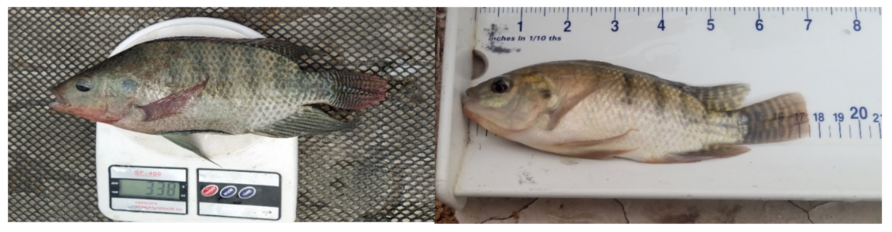
Figure 2.
In the left, lateral scheme of the pond with Biosonics 201 kHz transducer and its beam. In the right, picture of real pond used.
Figure 2.
In the left, lateral scheme of the pond with Biosonics 201 kHz transducer and its beam. In the right, picture of real pond used.
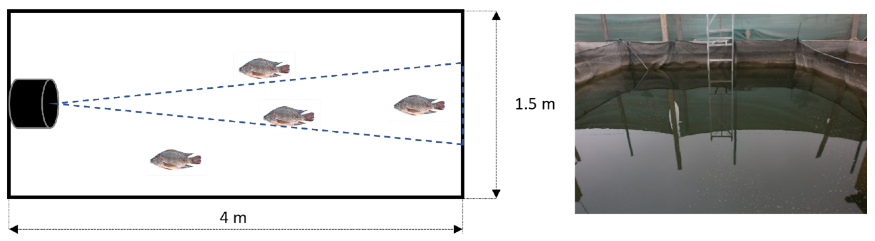
Figure 3.
In the left, echogram and TS profile of one trace belonging to group 7. In the right, echogram and TS profile of one trace belonging to group 8. All images were obtained from Sonar5-Pro software.
Figure 3.
In the left, echogram and TS profile of one trace belonging to group 7. In the right, echogram and TS profile of one trace belonging to group 8. All images were obtained from Sonar5-Pro software.
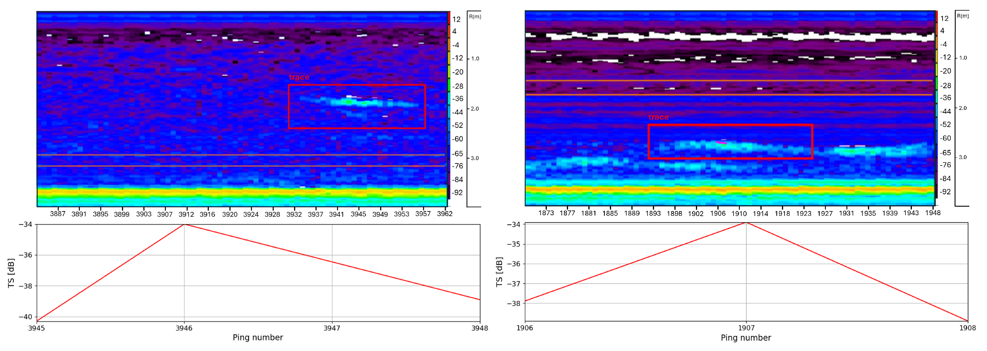
Figure 4.
Left: X-ray of a tilapia with total length 27 cm in lateral (up) and dorsal view (bottom). Grey shadows correspond to the extracted 2D orthogonal masks of the swimbladder, red lines mark the best elliptic fitting for the swimbladder masks in the two aspects. Right: Virtual sources (red) and collocation points (blue) in the MFS numerical model for calculating the acoustic backscattering of the Nile tilapia’s swimbladder, lateral (up) and dorsal (bottom) views.
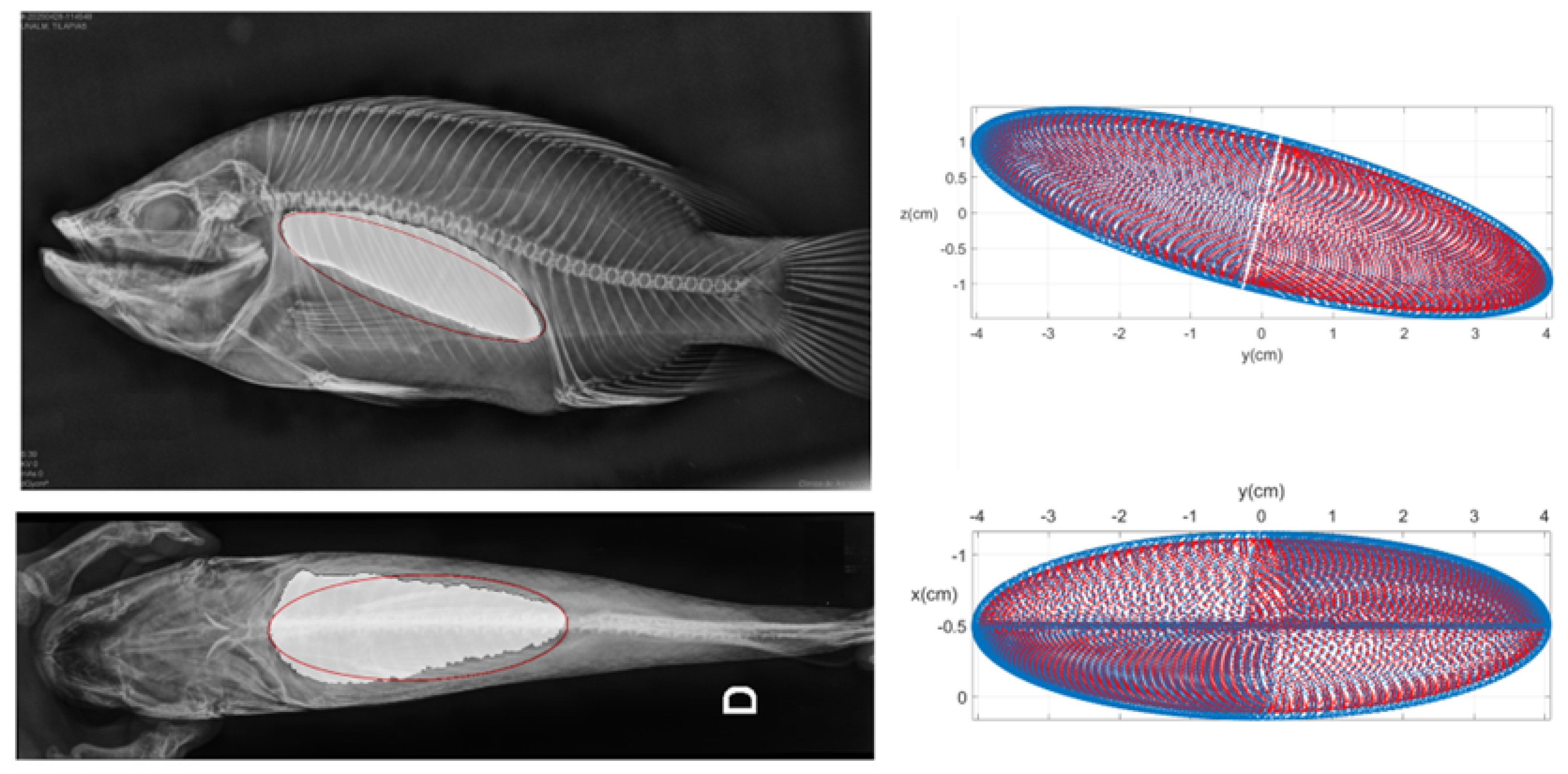
Figure 5.
Top: violin plot from Tmax distributions for the different size groups and linear regression for TSmax – TL. Bottom: violin plot from TSmean distributions for the different size groups and linear regression for TSmean -TL linear regression on the bottom. Black continuous line corresponds to the experimental data fit,discontinuous red line to the numerical fitting, and dashed black lines indicate the 95% prediction bounds of the experimental data fit.
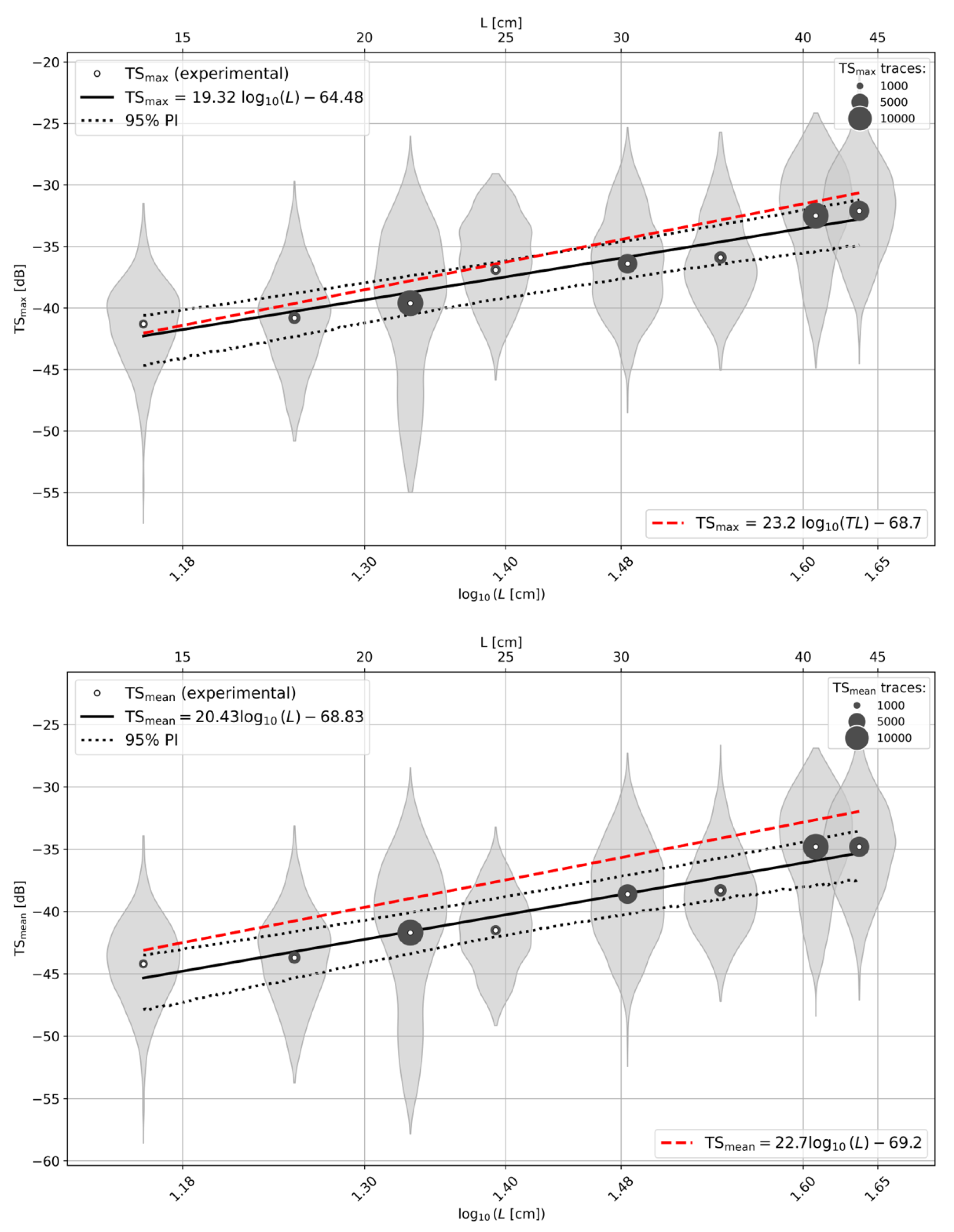
Figure 6.
The figure shows the data obtained from X-ray images, the potential fit, and the 95% prediction intervals for swimbladder length (SBL, left) and swimbladder volume (SBV,right) as a function of the total length of the fish (TL).
Figure 6.
The figure shows the data obtained from X-ray images, the potential fit, and the 95% prediction intervals for swimbladder length (SBL, left) and swimbladder volume (SBV,right) as a function of the total length of the fish (TL).
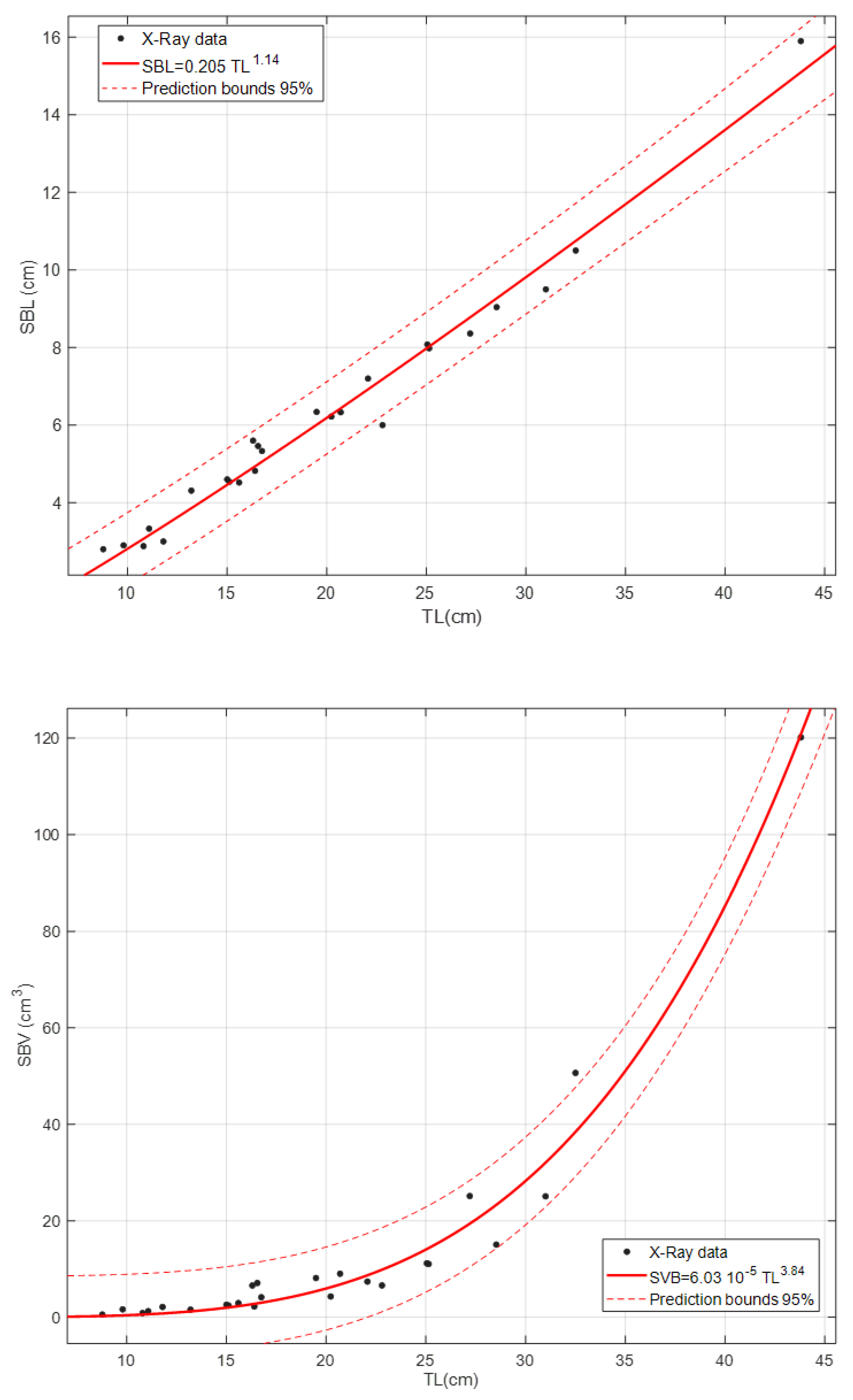
Figure 7.
The figure shows the data obtained from X-ray images, the potential fit, and the 95% prediction intervals for the maximum lateral cross section of the swimbladder (SBCS) as a function of the total length of the fish (TL).
Figure 7.
The figure shows the data obtained from X-ray images, the potential fit, and the 95% prediction intervals for the maximum lateral cross section of the swimbladder (SBCS) as a function of the total length of the fish (TL).

Figure 8.
Directivity of the TS from swim bladder prolate sphere model corresponding to a TL=27 cm Nile tilapia. Angle denotes the relative angle between the fish axis and the beam propagation direction. Dashed lines signal the limits of the swimming direction considered.
Figure 8.
Directivity of the TS from swim bladder prolate sphere model corresponding to a TL=27 cm Nile tilapia. Angle denotes the relative angle between the fish axis and the beam propagation direction. Dashed lines signal the limits of the swimming direction considered.
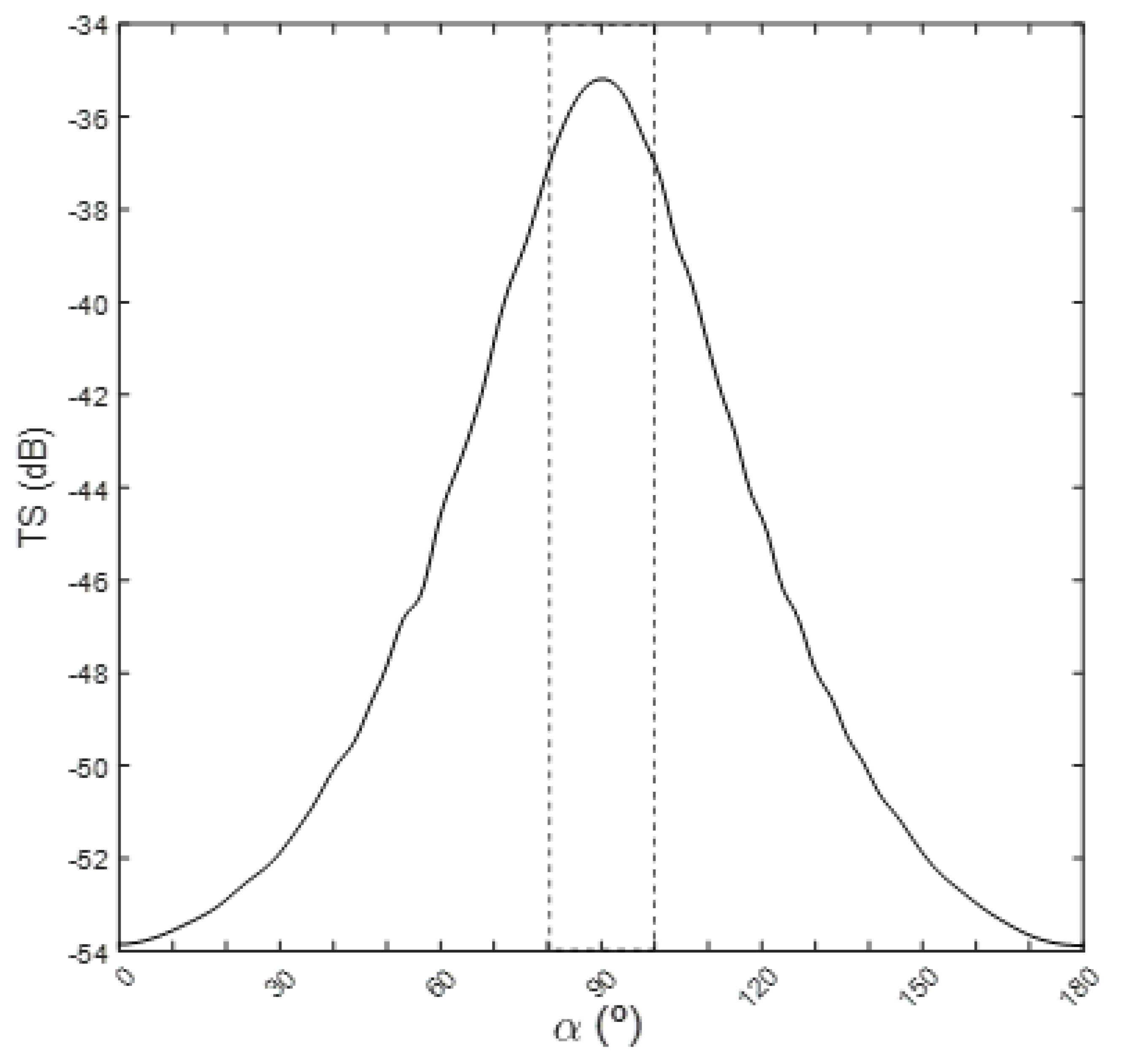

Table 1.
Fish group data.
| Group | Fish number | Mean TL (cm) | Min TL(cm) | Max TL(cm) | Mean W(g) | std W(g) |
|---|---|---|---|---|---|---|
| 1 | 20 | 14.1 | 13.0 | 15.0 | 47 | 10 |
| 2 | 15 | 17.9 | 17.0 | 19.0 | 99 | 7 |
| 3 | 14 | 21.5 | 21.0 | 22.0 | 180 | 8 |
| 4 | 14 | 24.6 | 24.0 | 25.0 | 230 | 16 |
| 5 | 6 | 30.3 | 29.0 | 31.0 | 540 | 60 |
| 6 | 6 | 35.1 | 34.0 | 36.0 | 760 | 60 |
| 7 | 6 | 40.8 | 40.0 | 41.5 | 1380 | 20 |
| 8 | 6 | 43.7 | 43.0 | 44.0 | 1450 | 110 |
Table 2.
Selected settings for DT-X Biosonics echosounder.
| Parameter | Value |
|---|---|
| Frequency | 201 kHz |
| Beam width | 9.9∘ |
| Pulse length | 0.1 ms |
| Ping rate | 5 pings·s−1 |
| Source level | 202.3 dB rel. 1Pa @ 1m |
| Receiver Sensitivity | −64.9 dB |
Table 3.
Average, median and standard deviation values from and distributions of each Nile tilapia group.
Table 3.
Average, median and standard deviation values from and distributions of each Nile tilapia group.
| Group | Mean TL | (dB) | (dB) | Number | ||||
|---|---|---|---|---|---|---|---|---|
| (cm) | Avg. | Med. | SD | Avg. | Med. | SD | of traces | |
| 1 | 14.1 | −44.2 | −44.0 | 3.4 | −41.3 | −41.0 | 3.5 | 1402 |
| 2 | 17.9 | −43.7 | −43.5 | 3.6 | −40.8 | −40.6 | 3.8 | 2240 |
| 3 | 21.5 | −41.7 | −40.6 | 5.7 | −39.6 | −38.6 | 6.0 | 8696 |
| 4 | 24.6 | −41.5 | −41.4 | 3.4 | −36.9 | −37.1 | 3.7 | 1698 |
| 5 | 30.3 | −38.6 | −38.7 | 4.0 | −36.4 | −36.4 | 4.0 | 5088 |
| 6 | 35.1 | −38.3 | −38.5 | 3.4 | −35.9 | −36.3 | 3.7 | 2291 |
| 7 | 40.8 | −34.9 | −34.4 | 4.5 | −32.5 | −31.9 | 4.6 | 8612 |
| 8 | 43.7 | −34.8 | −34.7 | 3.8 | −32.1 | −32.0 | 3.8 | 5400 |
Table 4.
Parameters () of the potential fits of the morphometric variables of the swim bladder (SBL, SBV, SBCS) as a function of the total length of the fish. Values in parentheses indicate the 95% confidence bounds for b.
Table 4.
Parameters () of the potential fits of the morphometric variables of the swim bladder (SBL, SBV, SBCS) as a function of the total length of the fish. Values in parentheses indicate the 95% confidence bounds for b.
| Fit | a | b (95% CI) | |
|---|---|---|---|
| 0.205 | 1.14 (1.07, 1.21) | 0.98 | |
| 3.84 (3.50, 4.18) | 0.97 | ||
| 0.0105 | 2.62 (2.39, 2.86) | 0.96 |
Disclaimer/Publisher’s Note: The statements, opinions and data contained in all publications are solely those of the individual author(s) and contributor(s) and not of MDPI and/or the editor(s). MDPI and/or the editor(s) disclaim responsibility for any injury to people or property resulting from any ideas, methods, instructions or products referred to in the content. |
© 2026 by the authors. Licensee MDPI, Basel, Switzerland. This article is an open access article distributed under the terms and conditions of the Creative Commons Attribution (CC BY) license (http://creativecommons.org/licenses/by/4.0/).
Copyright: This open access article is published under a Creative Commons CC BY 4.0 license, which permit the free download, distribution, and reuse, provided that the author and preprint are cited in any reuse.


