
Submitted:
16 June 2025
Posted:
16 June 2025
You are already at the latest version
Abstract
Fish stocks and their management are paramount for sustainable fisheries under the ongoing changes in atmosphere-sea interactions. The Aegean Sea, one of the composite seas influenced by different water masses, is characterized by a diverse ecosystem. Small pelagic fish are abundant and tend to form schools that vary in size. One of the most efficient and rapid techniques for sampling fish schools over a large area is the use of acoustic methods. Therefore, an acoustic survey was conducted in the coastal areas along the entire Turkish Aegean waters between June and August 2024, using a scientific quantitative echosounder equipped with a split-beam transducer operating at 206 kHz. During the survey, environmental parameters including water physics, optics, and bathymetry were measured at 321 stations. Additionally, satellite data were used to obtain water primary production levels for each sampling month across the entire study area. Using a custom computer algorithm written during the present study in MatLab, fish schools were automatically detected to measure various morphological and acoustic features. Through a series of statistical analyses, three optimal clusters were identified, each characterized by specific morphological, acoustic, and environmental variables associated with different areas of the study. School morphology and acoustic properties also varied with bottom depth. Cluster 1 was mostly found in open and relatively deep waters. Cluster 2 appeared in areas impacted by anthropogenic sources. Principal Component Analysis (PCA) revealed that the first component (PCA1) was correlated with school height from the bottom (HFB) and overall school height (SH), followed by minimum depth (MnD), maximum depth (MxD), and volume backscattering strength at the school edge (SvE). The second component (PCA2) was associated with school width (SW) and area (A). Cluster 1 was characterized by schools with large SW and A, and relatively high HFB and SH. Cluster 2 showed low HFB and SH, while Cluster 3 had high MnD and MxD and low SvE. Based on the descriptors for these clusters, each cluster could be attributed to fish species at different life stages, namely sardine, horse mackerel, and chub mackerel, distributed along the entire Turkish Aegean coast.
Keywords:
fish school
; small pelagics
; acoustics
; morphs
; environment
; Aegean coastal waters
1. Introduction
Fish play a crucial role as a source of food, a key component of ecosystems, and a driver of the economy in aquatic environments. Among these, marine systems contribute more significantly than other aquatic environments, primarily due to their larger volume and area [1]. However, sustaining these ecosystems over time has become increasingly challenging due to various atmospheric-sea interactions and anthropogenic impacts [2]. These factors have notably influenced fish populations in marine ecosystems, particularly under conditions of global environmental change [2–4].
Fish schools are typically composed of pelagic species, although some demersal fish may also form bottom-dwelling swarms. Large schools are more commonly formed by small pelagic fish than by larger species [5,6]. School size tends to be inversely related to individual fish size, larger schools often consist of smaller fish [7,8]. This trend is related to the evolutionary advantage of small-sized, r-selected species, which have distinct population dynamics and biological traits compared to larger, k-selected species. Schooled fish have developed complex behavioral mechanisms to defend against predators in the marine environment [9]. These behaviors reduce predation risk under adverse conditions [10], as the fish swim in a coordinated manner relative to their nearest neighbors.
Schooling behavior is generally influenced by the trophic conditions of the marine environment and is rarely observed in ultra-oligotrophic areas, where the food chain dynamics differ. Large schools are often found in eutrophic regions, coastal zones, and open waters where upwelling systems, riverine inputs, and anthropogenic nutrient influx enhance primary productivity [3,11–15]. However, the timing and extent of schooling depend on the specific biological requirements of each species [5,16,17]. Eutrophic regions such as the Mauritian coast, the Black Sea, and the western Mediterranean are notable examples [6,18,19]. Under favorable marine conditions, such as adequate visibility, absence of predators, and suitable physical parameters, large pelagic fish often follow schools for feeding, spawning, and nursery purposes during migration [1]. Historically, the ultra-oligotrophic waters of the eastern Mediterranean (e.g., the Levantine Sea) lacked small pelagic fish schools. However, over the past two decades, sardine schools have been observed once a year in the Levantine coastal waters, typically in May, likely due to increased anthropogenic nutrient inputs [20].
Overall, fish school morphology can vary depending on species, environmental conditions, and disturbances caused by vessel presence and avoidance behavior [14,21–26]. Different school shapes can be attributed to such factors and provide descriptive information for interpreting and evaluating fish schools [27]. The number and size of fish can also vary depending on their position within the schoo, whether at the edge, periphery, center, or as leading individuals during movement [1,5,22,27]. In addition to specific school forms, their position in the pelagic environment also varies, affected by bottom depth, distance from the surface and seabed, proximity to the bottom, predator presence and behavior, fishing activity, and gear type [1,28–30]. Tsagarakis et al. [8] used similar school morphology descriptors and fractional parameters for sardines. Most small pelagic species are generally distributed close to the coast, over the continental shelf, and undertake well-defined seasonal migrations [17]. Sardines, anchovies, mackerel, and horse mackerel migrate towards coastal areas in summer and retreat to deeper waters in winter [11]. Furthermore, Georgiadis et al. [13] noted the appearance of dense bogue shoals close to the shoreline at night around island communities in the Aegean Sea.
Fish schools can be visualized using various systems such as video/cameras, acoustic technologies (passive, active, and tagging), satellites, and LIDAR/RADAR, to measure their morphology [3,5,8,10,24,28,31,32]. Each system has specific advantages and limitations. Primary differences include sampling coverage, aspect ratio, effort, and depth penetration, followed by data types and variables. These factors also vary with school morphology and fish size under different atmospheric and sea conditions [23]. Among these, acoustic instruments are among the most cost-effective tools for sampling schools. They provide various types of data suited to both scientific and non-scientific purposes [4,24,30,33,34]. There are two main types of acoustic sampling systems: SONAR (Sound Navigation and Ranging), which samples in 2D using a tilted beam [35–37], and echosounders, which provide 1D sampling, either vertically or side-looking [38,39]. Scientific acoustic systems using dual- and split-beam transducers generate quantitative data depending on system properties, including vertical and horizontal resolution [6,24]. Although the initial cost of acoustic systems can be high, they become cost-effective over time due to their efficiency. Advantages include high sampling speed, broad coverage, repeated sampling at the same location, and effective operation under poor sea/air conditions [24]. However, disadvantages include difficulty in species identification, frequency-dependent size detection, and limited depth penetration, challenges also noted in zooplankton studies [40–42] and fish behavioral studies [43]. To overcome these issues, multi-frequency systems are often used during fieldwork, and ground-truthing is required to identify the species observed [24,44–47]. Depending on spatial resolution, sampling strategies can be adjusted to better capture both vertical and horizontal dimensions of schools. Despite the disadvantages, acoustic systems are the most widely used technology [4,6]. These disadvantages have been mitigated through advances in software, algorithms, in situ/ex situ experiments, and improved methodologies using advanced programming languages and analytical protocols. e.g. SHAPES, Frequency Response, EchoView, SCHOOL, PosiBIOM [27,32,39,44,48–51].
The Aegean Sea, one of the largest seas in the Mediterranean Basin, is shallower compared to other regions. In terms of air-sea interactions that affect small pelagic fish schools, it represents a cosmopolitan water mass [2]. The Aegean Sea is influenced by inflows from the Black Sea via the Turkish Straits system and circulation patterns connected to the Atlantic-derived Mediterranean waters. Atmospheric and oceanographic interactions, both seasonal and annual, affect water circulation in the Aegean [52]. In addition to global changes [2], regional dynamics within the Mediterranean, particularly from the Levantine Sea, also influence water mass structure in the Aegean.
The Turkish Aegean coastline, although limited by maritime borders with Greece, has the longest stretch of Turkish marine coastline and significant potential for fish schools, depending on water productivity and fish biology. Sardines dominated pelagic fish populations from 1978 to the 2000s, followed by Trachurus species [20]. More recently, sardines have had the highest catch volume in the Turkish Aegean Sea, surpassing other species from 2014 to 2023 (16,500–23,500 tonnes, [53]). Historically, fishery research in the Aegean has focused on population growth parameters rather than school morphology or acoustic structures. Most data have been derived from commercial fisheries and landing records, with limited input from scientific surveys. No acoustic studies have been conducted in Turkish Aegean waters. In contrast, Greek studies have focused on ontogenetic shifts [8], acoustic stock assessments [54–57], and school structures [49,58,59]. In Turkey, a few studies have addressed school aggregation and tracking around artificial reefs.
Therefore, the present study aims to analyze the morphology (shape, school height, width, area, distance from the bottom, minimum and maximum depth) and acoustic structure (volume backscattering strength and coefficient, backscattering values at the edge and interior, their mean, min/max values, and Target Strength) of pelagic fish schools in vertical depth profiles along the Turkish Aegean coast during summer (June–August). This structure is further related to environmental parameters (physical water properties, primary productivity, and optical properties), as well as school classification across six bottom depth categories along the entire and segmented coastline.
2. Materials and Methods
The materials and methods included the collection of acoustic data, surface and near-bottom physical water data, and statistical analyses for recognizing shapes and estimating morphometric and acoustic variables of fish schools in space and time during June–August 2024 (a commercially non-fishing season) along the Turkish Aegean coastal waters (Figures 1 and S1).
2.1. Data Collection
2.1.1. Acoustics
Acoustic data were collected using a quantitative scientific echosounder (DT-X, BioSonics Inc.). The echosounder operated at a frequency of 206 kHz with a split-beam transducer and was integrated with a differential GPS (GARMIN) (Table 1). Prior to data collection, the echosounder was calibrated using a 0.4 ms pulse width, referencing a calibration tungsten ball provided by BioSonics Inc.
The research cruise started in the south and concluded in the north of the study area, lasting three months (June–August 2024) (Figure S1). Acoustic tracklines were spaced at horizontal intervals of 100–500 m, covering bottom depths from 10 m to 70 m, and extending up to 200 m in some cases (e.g., for benthic and plankton studies) or as shallow as 5 m depending on navigational constraints. The vessel maintained a speed of 5 nautical miles per hour during the survey (Figure 1, Figure 2, Figure 3, Figure 4, Figure 5 and Figure 6 and Figure S1). The echosounder transmitted 0.1 ms pulses at a rate of 5 pings per second, depending on the maximum depth settings (Table 1). Data were recorded using BioSonics Visual Acquisition software (version 6.3.1.10980). At intervals, the transducer was switched to passive mode to record background noise, which was used to determine the minimum threshold during data processing. The total data volume was approximately 141 GB, comprising around 1,600 files, each about 30 minutes in duration. The total navigated distance covered during the study was approximately 4,550 nautical miles.
2.1.2. Environments
During the survey, a total of 321 stations were sampled for physical variables (temperature, salinity, conductivity, dissolved oxygen, pH, and total suspended matter) in both surface and near-bottom waters (Figure. S1). Samples were taken using a 5 L Nansen bottle from the surface and from near-bottom layers, 2–3 meters above the seabed. The physical parameters were measured using a portable multi-parameter probe (HACH HQ40d model).
For optical variables, Secchi disk depth was measured at each station. Additionally, photosynthetically active radiation (PAR) was measured vertically from the surface to a depth of 50 meters (the cable length), using a spherical sensor (SPQA-4671 model, LI-COR, Inc.) and a multiparameter recorder (LI-1400 model).
Monthly averaged surface chlorophyll-a distribution at a 4 × 4 km resolution for June, July, and August 2024 along the coastal region of the study area was provided by Prof. Dr. Ahmet Cemal Saydam from https://oceandata.sci.gsfc.nasa.gov.
All environmental parameters can influence the occurrence and distribution of fish schools.
2.2. Data Processing
2.2.1. Acoustics
The acoustic data were processed in two stages: pre-processing andpost-processing.
Pre-processing: The data were analyzed using BioSonics Visual Analyzer software (version 4.3.0.9020), which converted the raw .dt4 files to ASCII .csv format. A threshold of -130 dB was applied, and ping-to-ping horizontal resolution was included in the output. Vertical resolution (based on count intervals, minimum resolution ~1.8 cm depending on depth) was set individually for each file. Visual Analyzer can define up to 349 strata from the surface to the maximum depth per file, and all settings were configured accordingly. The output data included volume backscattering strength (Sv in dB) in .csv format. These settings allowed for high spatial and Sv resolution (including zooplankton layers), which were then used for post-processing in MATLAB (version 2021a, MathWorks).
Post-processing: Using the PosiBiom package [51], missing or misidentified bottoms were corrected, an essential step before acoustic data analysis in hydroacoustic studies. A MATLAB script was written to further process the pre-processed data, distinguishing fish schools from other scattering layers (e.g., zooplankton). The algorithm included criteria for identifying meso- and macro-scale fish schools based on lateral area, while filtering out small samples, surface/volume/bottom reverberations, interference, and bottom-touching schools. If a false bottom (> -30 dB) remained, the script removed it.
Adjacent schools were discriminated by accounting for data gaps. The following criteria were applied:
- School identification using Sv values between -50 and -33 dB
- School separation: fewer than 20 successive vertical counts or horizontal pings indicates the same school; otherwise, it is a separate school
- Exclusion of small sample schools: schools with fewer than 20 echoes
- Exclusion of small area schools: schools with lateral areas smaller than 20 m²
After filtering, basic acoustic (Elementary Distance Sampling Unit, EDSU; [24]) and morphometric variables (in meters) were derived for statistical analysis. These variables included: (Please look at the MatLab, 2021a for the detail of each own command for the following estimates, *: after conversion of backscattering strength to coefficient, the mean values were calculated, and +: identical and effective variables involved into the statistical analyses):
- i.
- School shape: defined by amorphous polygons in meters (depth and geographic distance)
- ii.
- A: School lateral area (m²), +
- iii.
- SH: School height (m), +
- iv.
- SW: School width (m), +
- v.
- SvE (dB/m³): Sv at polygon edge (min, max, mean*), +
- vi.
- SvI (dB/m³): Sv inside polygon (min, max, mean*),
- vii.
- Sv (dB/m³): Total Sv of polygon (min, max, mean*),
- viii.
- HFB (m): Height from bottom to the school's deepest point, +
- ix.
- MnD (m): Minimum (shallowest) school depth from the surface, +
- x.
- MxD (m): Maximum (deepest) school depth toward bottom, +
- xi.
- Sa / sa (dB/m² and m²/m²): Backscattering strength and coefficient per unit area, +
- xii.
- Sv / sv (dB/m³ and m²/m³): Volume backscattering strength and coefficient per unit volume, +
- xiii.
- NASC (m²/nm²): Nautical Area Scattering Coefficient, +
- xiv.
- TS (dB/individual): Target strength
TS was converted to fish length using Love’s formula [60].
2.2.2. Environment
Among the environmental parameters, the PAR (Photosynthetically Active Radiation) value reaching the seabed was calculated using a well-known exponential light attenuation equation, established individually for each station.
2.3. Statistical Analyses
2.3.1. Acoustics
Using a normalized and consistent data matrix derived from the acoustic data, a series of statistical analyses were conducted to estimate the spatiotemporal structure of fish schools. To determine the optimal number of clusters, a silhouette analysis was applied to the data matrix. Based on the silhouette results, a k-means clustering analysis was performed using the specified number of clusters. Significant variables were identified for each cluster, and each cluster was then color-coded and plotted on a map to illustrate its spatial distribution. To assess multicollinearity among variables, a Principal Component Analysis (PCA) was applied to the data matrix. To evaluate the statistical significance of the cluster separation, a Canonical Analysis of Principal Coordinates (CAP) was performed. Furthermore, bottom depth intervals of 10 m (±5 m), 20 m, 30 m, 50 m, 70 m (±5 m), and ≥80 m were selected to investigate depth-wise variations in key fish school descriptors. For each selected depth, corresponding variables were extracted to form a depth-specific data matrix. These matrices were subjected to PCA, followed by CAP. The relative contribution of each variable was visualized on the PCA configuration using proportional sizing.
2.3.2. Environment
All environmental parameters were spatially visualized using contour maps, generated via Kriging interpolation. This method was selected based on a variogram analysis performed in SURFER 12 software (Golden Software).
3. Results
3.1. Study Area
3.1.1. Bottom Depth and Coastline Features
A key objective was to correct bottom depth data in order to accurately estimate the true depth, especially when isolating fish schools from the seabed and within the water column. Figure 2 shows the corrected depth data produced using the PosiBiom package, along with the acoustic survey tracklines used in this study.
The maximum depth surveyed was generally limited to 70 meters. In some areas, the ship turned back where the depth coincided with Greek territorial waters. However, on a few occasions, the vessel sailed in Turkish waters where bottom depths reached up to 200 meters. The 206 kHz sound frequency used in this study is capable of penetrating depths up to 250 meters, despite transmission loss due to sound attenuation over range. Steep cliffs were observed near the coastline (Figure 2). The study area includes large gulfs, bayous, and marine protected areas (MPAs), particularly within sectors 2, 10, 14, and 15 (Figure 1 and Figure 2). Most of the larger MPAs were characterized by marine cliffs (Figure 2).
3.1.2. Chlorophyll
Overall, chlorophyll (Chl) concentrations increased from June to August along the coast of the study area. Some local gulfs and coastal regions consistently exhibited high Chl concentrations, particularly the Gulf of İzmir, surrounded by the metropolitan city of İzmir, and areas with fish farms (Figure 2 and Figure 3). These elevated concentrations became especially pronounced over time, particularly in August. The Gulfs of Datça and Gökova had the lowest Chl concentrations, comparable to those along the Turkish Mediterranean coast. In June, the area near the Dardanelles Strait showed moderate Chl levels compared to July and August. This region was influenced by water flowing from the Black Sea through the Sea of Marmara. In locations where high concentrations were consistently observed, Chl levels expanded locally over time. For example, the Gulf of İzmir was completely covered with the highest Chl concentrations in August, when the sea took on a brownish-red hue that persisted and was followed by mass fish mortality. Additionally, the highest concentrations were also clearly observed near fish farms in August. These conditions triggered zooplankton blooms since the Aegean Sea is colder than the eastern Mediterranean and warms up later, which attracted small pelagic fish and promoted fish school aggregations.
3.1.3. Physics
During the survey, sea surface temperature varied between 20.5 and 28.5 °C across the entire study area, while near-bottom water temperatures ranged from 18 to 28 °C. Salinity showed a decreasing gradient from south to north throughout the study area, which was more pronounced in the near-bottom waters. Oxygen content and pH slightly increased from south to north, in contrast to total suspended solids (Figure 4). Cold water from the Black Sea, passing through the Sea of Marmara, was observed exiting the Dardanelles Strait into the Aegean Sea, whereas warmer water occurred in the northern part of the Aegean Sea. In this specific region, influenced by the Meriç River located at the northernmost part of the study area, less saline water was present compared to the southern part of the study area (Figure 4).
3.1.4. Optics: Secchi Disk Depth (m) and PAR
The maximum Secchi disk depth was recorded as 31.5 m near the Gelibolu Peninsula. In general, this depth increases from the coast toward the open sea. In some specific areas, especially near fish farms, the Secchi disk depth was measured to be low (Figure 5). Additionally, low depths were observed in regions dominated by Black Sea water. The minimum Secchi disk depth was 3 m at station P93, followed by 4 m at station P219 (Figures S1 and 5).
Since the absolute value of PAR reaching the bottom generally occurs at different times of the day and under varying weather conditions, fluctuations are expected in the percentage values. The analysis results are shown in Figure 5, where the values range between 3.243 and 6.261 mol photon/cm²/s (equivalent to 324.3–626.1 µmol photon/m²/s). In certain regions (Datça, Gökova, the southern İzmir peninsula, and Edremit Bay along with its southern part), light intensity varies between 3 and 4 mol photon/m²/s. The highest light intensities reaching the bottom were recorded in the northern part of the study area (Figure 2 and Figure 5). Babakale (Edremit) and the Bodrum peninsula cape are locations with the highest PAR intensity from the sun.
3.2. Fish Schools
A total of 3,906 schools were detected after applying the filtering criteria. The number of schools tended to increase from south to north and decrease from coastal areas (< 70 m) toward open water (Figures S2–S16). Nevertheless, the probability of school occurrence was higher in regions with high surface chlorophyll content (>0.5 mg/m³) than in areas with lower chlorophyll (Figure 3 and Figure S17). The minimum number of schools was found in the Datça and Gökova gulfs, where chlorophyll levels were lowest. Besides the primary effect of chlorophyll, fish schools appeared to prefer warmer waters, above 21 °C at the surface and 24 °C near the bottom, and occurred more frequently under these conditions (Figure 4 and Figure S17). Salinity did not affect the frequency of fish school occurrence. For example, in Saroz Gulf and around the exit of the Dardanelles Strait in the Aegean Sea, where Black Sea salinity prevails, fish schools were frequently observed. Optical parameters were also found to be related to fish school occurrence (Figure 5 and Figure S17). Furthermore, the estuarine influence of the Meriç (Greek border in the north, sector 15), Gediz (in Izmir Gulf, sector 10), and Menderes (sector 5) rivers appeared to increase the number of fish schools (Figures 1,2 and S17).
3.2.1. Morphometrical Structure
The morphometrical structure mainly consisted of two substructures: the school’s own structure and depth-related structures. Figure 6 shows an example echogram containing a fish school, interference caused by the ship’s echosounder, and weak scattering layers (a), the corresponding filtered echogram (b), and different types of fish schools observed throughout the study (c) (Figures S2–S17). Morphometries of the fish schools varied depending on factors such as bottom depth, distance from the coast, regional productivity, locations of anthropogenic effects, and ship avoidance behavior (Figure 1 and Figures S2–S17). At greater depths (maximum school depth > ~20 m), the shape and movement of the school relative to the ship's heading tended to move downward over time and distance (Figure 6c). This trend was more evident for larger schools. In near-coastal areas, the opposite pattern was observed compared to those at greater depths (Figure 6c and Figures S2–S17). Sometimes, schools were dispersed both vertically and horizontally, forming a rectangular shape (Figure 6c and Figures S2–S17).
3.2.2. School Morphs
The maximum school height (SH) was measured at 46.5 m, but overall it was about 30 m (Figure 7). The minimum value was less than 5 m. Based on the sectors, high fish schools were observed in sector 14, followed by sectors 6, 7, and 8 (Figure 1 and Figure 7). Moderate heights (10–15 m) were partially found in sectors 1, 2, and 12, where greater depths occurred (Figure 2). Furthermore, with the exception of sectors 1 and 2, the moderately productive regions had fish schools of high and moderate height (Figure 3 and Figure 7). Sectors 3, 4, 5, and 9 had taller schools, followed by sector 2, compared to the other sectors (Figure. S18). Beyond sector 5 northward, school height was positively correlated with the distance from the bottom to the school (Figure S18).
A maximum school width (SW) of 549.7 m was recorded, though typically it measured around 100 m (Figure 7). Overall, school widths showed a spatial distribution distinct from school heights, particularly at greater depths. Widths frequently ranged between 30–50 m. These observations suggest that fish school morphology is influenced by bottom depth: in shallow waters, schools spread more horizontally, while at greater depths, vertical dispersion becomes more significant. This highlights the importance of vertical school area in school dispersion. Excluding non-productive sectors (1 and 2) (Figure 3), SW was positively correlated with school area. The SW distribution was left-skewed across all sectors, with narrower schools predominating (Figure S18).
The largest estimated school area (A) was 5722.4 m², although most schools measured around 300 m² (Figure 7). Small, scattered schools occurred in highly productive areas characterized by high turbidity, low photosynthetically active radiation (PAR), and shallow Secchi disk depth (Figure 3, Figure 5 and Figure 7). Bottom depth also influenced the occurrence of small schools (Figure 2 and Figure 7). Similar to SW, small-sized school areas dominated all sectors.
However, none of the acoustic structure variables correlated with school morphology metrics.
3.2.3. Depth-Related Morphologies
The maximum HFB reached 59.2 m, generally around 40 m (Figure. 8a). Depending on bottom depth, HFB was predominantly measured within 10–20 m, indicating schools positioned near the bottom, and spatially at depths greater than 20 m in various sectors. This deeper positioning overlapped with warmer surface waters (Figure 4a and Figure 8). In the first two and last three sectors, schools were found at greater depths (closer to the surface), while in other sectors, schools were shallower (closer to the bottom). HFB was mostly correlated with school height (SH), with most schools located near the bottom (Figure S18).
3.3. Spatial Distribution
The MnD showed a spatial distribution pattern contrasting with the HFB but aligned with the MxD. This suggests that fish schools were dispersed, extending to greater bottom depths where small-sized schools dominated (Figure 8). A correlation existed between MnD and MxD, though neither correlated with other variables (Figure S18). Most sectors exhibited distribution histograms of MnD and MxD centered around their average values (Figure S18).
Acoustical Structure
Key echo data sampling unit (EDSU) parameters observed included volume backscattering strength (Sv or sv) per unit volume (m³), and area backscattering coefficients (Sa or sa) per unit area (m²), along with numerical abundance (NASS or NASC in nm²) (Figures 9 and S19). These variables characterize the basic structure of fish schools, reflecting fish density or size at the edge and inside the school, influenced by spatial and ambient conditions during ship approach.
Sv at the Edge of Fish Schools (SvE, dB/m³): SvE ranged between -58 and -35 dB, differing notably between the north and south of the İzmir Peninsula (Figure 9). Generally, northern areas showed higher SvE values, indicating denser or larger fish schools. In the north, SvE contrasted with the internal Sv, while in the south, SvE and internal Sv were similar (Figure 9). SvE correlated only with the school’s internal sv (Figure S18). Histograms showed a normal distribution of SvE across all sectors (Figure S18).
Sv Inside Fish Schools (Sv, dB/m³): Sv inside the schools fell within expected ranges for the fish species studied (Figure 9 and Figure S19). Typically, Sv values exceeded -53 dB, reaching up to -35 dB throughout the study area. The distribution of Sv was left-skewed in all sectors (Figure S18).
Backscattering Strength per Unit Area of Fish School (Sa) in dB/m²: Sa exhibited a spatial distribution similar to that of Sv. This parameter is essential for illustrating the distribution of fish schools throughout the integrated water column and reflects the relative fish abundance in space (see Figures 9 and S19).
Nautical Acoustical Scattering Strength of Fish School (NASS) in dB/nm²: Since fish schools can span large sea areas, NASS is often employed to indicate the relative fish school abundance over these larger spatial extents (see Figures 9 and S19).
Target Strength (TS): TS was used to estimate the size distribution of fish, with a histogram of weak scatterers observed in the TS range of -65 to -25 dB (Figure S20). Generally, TS values less than -60 dB, corresponding to fish smaller than 5 cm in length, dominated the fish populations across all sectors. In some sectors (1, 4, 9, 12, and 14), TS values between -50 and -40 dB (estimating fish lengths of 10–15 cm) showed secondary peaks in the frequency histograms (Figure S20). These sectors coincided with eutrophic regions. Some sectors contained larger fish ranging from 15 to 30 cm (Figure S20). However, it is important to note that TS measurements do not provide absolute counts of individuals because TS is recorded for single targets detected according to pulse shape and pulse width criteria, which makes measurements in dense schools less reliable.
3.4. Statistical Structure
3.4.1. Fish Clusters
Using silhouette analysis, the optimal number of clusters for the statistical data matrix was determined to be three. The total silhouette sum of distances was estimated at 1317.38 after iterations testing different cluster numbers, with each of the three clusters having silhouette values above 0.5 (Figure 10a). Among these, cluster 3 formed a distinct group, separate from clusters 1 and 2 (Figure 10b). Clusters 1 and 2 showed overlapping distributions, indicating shared morphometric and acoustical characteristics (Figure 10b).
The fish school associated with cluster 3 predominated in the northern part of the study area, extending northward from the Izmir peninsula (Figure 11). In contrast, sectors 1 and 2 were generally devoid of cluster 3 schools. Cluster 1 was primarily found in open and relatively deep waters, while cluster 2 appeared mainly in areas influenced by anthropogenic sources (Figure 11).
Cluster 1 was characterized by schools positioned higher above the bottom, exhibiting greater school height but lower volume backscattering strength (Sv). Cluster 2 consisted of schools with high Sv values concentrated at the edges, located near the bottom, and with low school height. Cluster 3 schools exhibited low edge Sv (SvE), but high MnD and MxD, indicating a more dispersed distribution yet relatively larger school size compared to the other clusters (Table 2).
The Principal Component Analysis (PCA) revealed trends in the variables consistent with the clustering results obtained from k-means (Figure 12, Table 2). PCA effectively discriminated between clusters by identifying the key variables that classify the fish schools within the study area (Figure 12). Regarding explained variance, the first principal component (PCA1) accounted for 28.7% of the variance, primarily influenced by linearity, along with the axes of HFB and SH. Other variables such as MnD, MxD, and SvE had lower discriminatory power on PCA1 (Figure 12). The second principal component (PCA2) explained 22.76% of the variance and was mainly associated with school width and area, alongside variables that had low effects on PCA1.
Based on the distribution of schools along the PCA axes, Cluster 1 consisted of schools characterized by large width and area, with moderately high HFB and SH values. Cluster 2 included schools with low HFB and SH, while Cluster 3 grouped schools with high MnD and MxD but low SvE. Notably, the sa and sv within schools did not distinctly contribute to school classification (Figure 12).
PerMANOVA results indicated that the structural variables of fish schools differed significantly among clusters (F₂, 3903 = 651.14, p = 0.0020, p < 0.05).
3.4.2. Depth-Wise Structure Analysis
A total of 2,683 fish schools were detected after applying filtering criteria based on classified bottom depths. PCA results revealed a similar overall structure to the non-depth-wise PCA, but with an apparent inversion when compared (Figure 12 and Figure 13), suggesting that school morphology is associated with bottom depth.
Morphological variables; SH, MinD, MxD, and HFB, as well as the sa showed increasing dependence on bottom depth. Conversely, SW decreased with depth, while A varied locally and independently along the second PCA axis. SvE tended to increase with depth up to approximately 80 m before decreasing (Figure 13). The sv showed no consistent pattern relative to fish school structure.
PerMANOVA confirmed that fish school structural variables significantly differed with bottom depth across the entire study area (F₅, 2678 = 259.24, p = 0.0020, p < 0.05) and within each sector analyzed.
4. Discussion
Over the last four decades, pelagic fish, especially small-sized species, have been extensively identified and characterized using school morphology and acoustic energetic descriptors. These descriptors have been applied to acoustic data alone as well as in combination with catch data, environmental variables, and bathymetric information [62]. For example, Reid et al. [49] characterized fish schools and clusters based on morphological parameters (length, height, area, perimeter, outline rugosity), energetic parameters (acoustic backscatter energy, density, internal variability), and positional parameters (latitude, longitude, time, depth from surface, altitude from bottom). Petitgas et al. [5] used even more detailed descriptors, including school cross-sectional area, total acoustic backscatter energy as an index of biomass (m² nmi⁻²), depth (distance from sea surface to school center), number of clusters, summed cluster lengths relative to survey length, average school number per km within clusters, and survey biomass and school number estimates.
In the present study, all these data types were utilized for statistical analyses, except catch data from trawl or purse seine fishing. During the survey, we caught chub mackerel, horse mackerel, and bogue using fishing rods, and observed sardine specimens caught by a fishing scoop.
The Mediterranean Sea, though generally oligotrophic, exhibits high habitat variability, making it an ideal environment to study the adaptive behavior of small pelagic fish under diverse environmental conditions [63]. Frequency of occurrence and morphometries of fish schools differed in relation to factors such as bottom depth, distance from the coast, ecosystem type, regional productivity, anthropogenic impacts, and ship avoidance. School shapes varied depending on bottom depth, and overall school structure was distinct between the northern and southern sides of the Izmir Peninsula, reflecting differences in hydrography, physics, and optics.
School morphology also changed with ontogeny; for instance, juvenile sardines formed more irregular, elongated, and rough schools that deviated from rectangular shapes, resembling ribbons, compared to adults [8]. Tsagarakis et al. [49] described schools of four species: anchovy schools were found closer to the bottom, across a wide bathymetric range exceeding 100 m, and had intermediate acoustic backscatter (Sv), size, and shape values relative to anchovy, blue whiting, mackerel, and round sardinella. Sardines, in contrast, occupied shallower waters and formed larger circular schools with higher Sv values than anchovy and other species [64]. Zwolinski et al. [65] observed contrasting characteristics for sardine occurrence in Portuguese waters, associating them with high chlorophyll a, low temperature and salinity, and low acoustic epipelagic backscatter, differing from Mediterranean patterns. Mackerel schools showed intermediate values across most descriptors, except rectangularity, where they deviated the most from rectangular shapes [64]. Sardine density centers tended to stabilize with increasing light intensity, with a wide range of preferred light levels. Abrupt vertical movements occurred at dawn and dusk, while depths remained relatively constant during intermediate daylight hours. Background light intensity was more influential on sardine behavior than the measured light intensity itself [64].
Beare et al. [66] found that afternoon anchovy schools exhibited higher acoustic backscatter (Sv) than morning schools, despite similar length, thickness, and area. Afternoon schools also tended to be closer to the seabed and had a narrower altitude range than morning schools [17]. Inshore anchovy schools had longer lengths and were distributed over deeper depths compared to offshore mixed schools, although average Sv, thickness, and area were similar [17]. Tsagarakis et al. [67] documented anchovy schooling disruption at night in the Aegean Sea, followed by school formation before dawn at shallow layers above the thermocline, with schools moving deeper near the seabed during daytime and returning toward the surface to disperse after dusk. D’Elia et al. [68] linked fish school position in the water column to seabed substrate type, with more pelagic behavior (schools farther from bottom) over softer seabeds and more demersal behavior (closer to bottom) over harder substrates. We observed similar structure characterizing fish schools occurred above the thermocline only in sector 9, moderately eutrophic region, mid and outer sectors with seagrass beds of Izmir Gulf with independence on the day time [69] (Figure. S10), but inner sectors (highly eutrophic and polluted region) inhabited schools at the greater depths on beds predominated with mud [69] (Figure. S11). Additionally, Boops boops shoals were observed near the shoreline during nighttime in anthropogenically modified areas and their distribution was influenced by location, season, and natural moonlight fluctuations in the Aegean Sea [13].
Giannoulaki et al. [70] used acoustical measurements combined with environmental data such as sea surface temperature (SST), chlorophyll-a (Chl-a), sea level anomaly, and depth to characterize the habitats of sardine life stages between the Gulf of Lions and the north Aegean Sea. Sardine juveniles were found in waters with SST between 21.5–24.5°C, Chl-a ranging from 0.345 to 2.718 mg m⁻³, sea level anomalies of 0–5 cm (particularly 1–3 cm), and depths shallower than 65 m during July. In the north Aegean Sea, sardine juvenile presence in June correlated with sea level anomaly of –6 to 0 cm, Chl-a of 0.47–1 mg m⁻³, depths <65 m, and photosynthetically active radiation (PAR) of 48–56 Ein m⁻² day⁻¹, consistent with conditions observed for small-area sardine schools. For anchovies, Giannoulaki et al. [71] reported that in summer and early autumn, adult anchovy were more likely found in waters less than 100 m deep with PAR <57 Ein m⁻² day⁻¹, SST <22°C, sea level anomalies of 2 to 6 cm, and in waters up to 180 m deep with sea level anomalies ranging from –5 to 12 cm and Chl-a between 0.5–7.4 mg m⁻³ across various Mediterranean regions including the north Aegean Sea. Juvenile anchovies were abundant in late autumn in waters <150 m deep, with sea level anomalies between –5 and 5 cm, SST of 17–19°C, and Chl-a of 0.36–2 mg m⁻³; and in winter, in shallower waters of 15–60 m with sea level anomalies between –8 and 10 cm, SST of 12–14°C, and Chl-a of 0.9–5.4 mg m⁻³.
Barra et al. [14] analyzed ecosystem factors and anchovy school densities from acoustical surveys across ten Mediterranean areas. They found that the spatial structure of anchovy and sardine schools is shaped by ecosystem characteristics and that total biomass changes follow a density-dependent mechanism. Among nine studied areas, anchovies in the Alboran Sea exhibited lower spatial variability (geostatistical coefficient of variation) in occurrence probability at high/medium densities compared to sardines.
In highly productive marine areas influenced by river runoff, fish populations tend to have spatially consistent and organized distributions due to localized enrichment mechanisms. Barra et al. [72] compared the summer spatial patterns of anchovy and sardine across two Mediterranean ecosystems: the upwelling Strait of Sicily and the freshwater-influenced North Aegean Sea shelf. They found that sardine spatial characteristics, such as spreading area and overlap with anchovy, differed notably between these ecosystems. Both species had higher occupation values in the upwelling area than in the shelf region. Biomass showed strong positive correlations with spatial metrics like occupation, aggregation, and patchiness across species and ecosystems. Overlap between anchovy and sardine increased with sardine biomass but decreased as anchovy biomass grew. Additionally, Bonanno et al. [63] highlighted that food availability and bottom depth preferences influenced the spatial distributions of both species in these ecosystems.
The spawning season of these two species can spatially influence their schooling behavior. Somarakis et al. [73] demonstrated that the preferred bottom depth for spawning ranged between 40 and 90 m in both the Ionian and Aegean Seas. However, sardines showed site selection differences, favoring areas with increased zooplankton abundance in the Aegean Sea during December, and regions with higher fluorescence in the less-productive Ionian Sea during February. In addition to these species, another species caught during the survey, Scomber japonicus, which possesses an air swim bladder and is therefore detectable by acoustic methods, was studied alongside Atlantic mackerel (Scomber scombrus), which lacks an air swim bladder. Giannoulaki et al. [74] investigated juvenile Atlantic mackerel occurrence in the Mediterranean Sea and found a high probability of presence associated with specific environmental variables. These included bathymetry, sea surface temperatures between 22 and 26°C, and circulation patterns indicated by sea level anomaly and absolute geostrophic velocity. Specifically, nursery grounds were characterized by waters shallower than 130 m, temperatures between 22 and 26°C, sea level anomalies from −6 to 0 cm, and velocities less than −0.1 m s⁻¹ or greater than 0.2 m s⁻¹. In deeper waters up to 220 m, nursery habitats corresponded to sea level anomalies of 6 to 8 cm and similar velocity ranges (< −0.1 m s⁻¹ or > 0.2 m s⁻¹).
In the study area, three distinct fish school clusters were identified based on school morphology, acoustic energy, and depth. Cluster 3 predominated in the northern part near the Izmir peninsula, while sectors 1 and 2 lacked this cluster. Cluster 1 was mostly found in deeper, open waters and characterized by schools positioned higher above the seabed with relatively high SH but low Sv. Cluster 2 appeared mainly in areas influenced by human activity, featuring schools with high SvE, near-bottom positioning, and low height. Cluster 3 schools showed low SvE, but larger mean and maximum distances between fish, indicating more dispersed but larger schools compared to the others. Principal component analysis revealed the first component was linked to HFB and SH, with other variables like MnD, MxD and SvE contributing less, while the second component involved school width and area but had low overall discriminative power. The study references Reid et al. [49], who used similar descriptive variables for clustering fish schools. Petitgas et al. [5] identified three principal components (PCs) in their analysis of school and cluster parameters. PCA1 reflected a contrast between school and cluster parameters, indicating that larger average school sizes were associated with fewer clusters, which also occupied a smaller portion of the surveyed area. PCA2 described the extent to which clusters were occupied by schools, while PCA3 was primarily related to the vertical distribution of the schools. In the present study, an additional structuring factor was identified: bottom depth. The PCA results showed a pattern similar to the non-depth-related PCA configuration described by Petitgas et al. [5]. However, school morphological variables (such as SH, MinD, MxD, and HFB) and the sa exhibited a clear dependence on bottom depth. The SW decreased with depth, while the A varied locally and independently of bottom depth along the PCA2 axis. The SvE tended to increase with bottom depth up to 80 m, after which it decreased. The sv values showed variability and did not consistently represent school structure. According to Muñoz et al. [22], statistical significance (explained variance >95%) was achieved with the third principal component in describing school characteristics. The first principal component was dominated by morphological variables; school length, height, area, and perimeter. In contrast, energy and density displayed less variability than the morphological descriptors. School density, and to a lesser extent school energy, were negatively associated with bathymetric variables, indicating that denser schools were typically found closer to the surface and in shallower waters.
Across all surveyed sectors, fish with target strength (TS) below -60 dB, corresponding to individuals smaller than 5 cm, were dominant. However, in eutrophic sectors (1, 4, 9, 12, and 14), a secondary peak appeared in the -50 to -40 dB range, indicating the presence of medium-sized fish (10–15 cm). Some sectors also contained larger fish exceeding 15 cm, up to 30 cm in length. In the eastern Mediterranean, sardines transition from juveniles (with low volume backscattering strength, Sv, and smaller morphological features) to adults at around 10.7 cm length [8]. For other pelagic species, horse mackerel TS ranges from -62 to -35 dB and chub mackerel from -61 to -30 dB across multiple frequencies [34,75]. Recent regressions at 38 kHz [76] relate TS to total length (TL) for anchovy as TS = 19.757·log(TL) – 74.78 (TS: -58 to -50 dB, TL: 8.3–13.5 cm), and for sardine as TS = 23.809·log(TL) – 75.82 (TS: -53 to -48 dB, TL: 9.1–13.8 cm).
All types of school descriptors are highly effective when acoustical variables are integrated with other parameters recommended in the literature. Giannoulaki et al. [56] evaluated the efficiency of these variables for defining school clusters and identifying fish species, considering the following key environmental and spatial descriptors:
- Enclosure index – the ratio of the length of the area's coastline to the length of the boundary line of the study area,
- Mean bottom depth,
- Coefficient of variation (CV) of bottom depth, and
- Subarea size, expressed in nautical miles².
The dependent variables included:
- (i) Range (as) – the maximum size of fish patches [77],
- (ii) Nugget effect (cop) – derived from omnidirectional variograms on a relative scale (cop/model variance, %),
- (iii) Surface area enclosed by the 100% standardized data variance contour,
- (iv) Anisotropy ratio – the ratio of the major to the minor axis of the best-fitted ellipse around the 100% variance contour,
- (v) Anisotropy direction – the tangent of the anisotropy angle of the major axis of the fitted ellipse, indicating how the maximum spatial structure of fish schools changes with direction,
- (vi) Surface ratio – the ratio of the area enclosed by 60% of the variance contour to that of the 100% contour, which quantifies the heterogeneity of fish school distribution. A low ratio indicates a heterogeneous spatial structure, whereas a high ratio suggests a more homogeneous distribution.
Giannoulaki et al. [58] distinguished between sardine and anchovy schools by applying stepwise multiple regression analysis to geostatistical parameters. For sardines, the analysis revealed that in summer, the size of the subarea was significantly related to the ratio of parameters, while the enclosure index was significantly related to the ratio in both summer and winter. In winter, the ratio was also significantly related to both the enclosure index and area. In contrast, no significant relationships were found for anchovy schools during summer. However, in winter, the ratio of geostatistical parameters was significantly related to certain topographic variables, including enclosure index, area, and bottom depth. Notably, smaller ratio values were observed in shallow, more enclosed, and smaller sub-basins. These results suggest that, for both species, the spatial organization of fish aggregations is influenced more by the geometric features of the area than by its absolute size.
5. Conclusions
This study represents the first comprehensive classification of small pelagic fish schools in Turkish marine systems, integrating acoustic, morphological, bathymetric, and environmental descriptors. After filtering, 3,906 schools were detected. School abundance increased from south to north and decreased with distance from the coast (>70 m). Two main morphometric components were identified: intrinsic school features and depth-related characteristics. Fish school morphology varied with environmental conditions such as bottom depth, coastal distance, regional productivity, anthropogenic impact, and ship avoidance. Schools were often dispersed both vertically and horizontally, with rectangular shapes observed. Average SH was approximately 30 m, peaking at 46.5 m. The maximum SW recorded was 549.7 m (typically ~100 m), and A reached up to 5,722.4 m², though it generally averaged around 300 m². Smaller, scattered schools were associated with high productivity areas, characterized by high turbidity, low PAR, and shallow Secchi depths. HFB correlated primarily with SH, and most schools were located near the seabed. MnD and MxD showed distinct spatial patterns, often contrasting with HFB. SvE ranged from -58 to -35 dB, with higher values in the north indicating denser or larger fish schools. In the north, edge and internal Sv differed spatially, whereas they were more consistent in the south. Overall, Sv values were typically higher than -53 dB.
All variables showed left-skewed distributions. TS data revealed a dominance of small scatterers (TS < -60 dB), corresponding to fish <5 cm in length. Cluster analysis revealed that:
Cluster 1 dominated deeper offshore waters, characterized by high SW and A.
Cluster 2 appeared in regions affected by anthropogenic sources, showing low SH and HFB.
Cluster 3 prevailed in the northern part of the Aegean, associated with high MnD and MxD but low SvE.
Principal Component Analysis (PCA) indicated that PC1 aligned with HFB and SH, followed by MnD, MxD, and SvE, while PC2 was driven by SW and A. Morphological and acoustic metrics (e.g., SH, HFB, sa) increased with depth, though SW decreased. School area varied locally, independent of depth. SvE increased with depth up to 80 m, then declined. Based on cluster descriptors, schools were tentatively linked to species: sardine, horse mackerel, and chub mackerel in different developmental stages along the Turkish Aegean coast. Anchovy presence was minimal, likely restricted to the northernmost areas.
Supplementary Materials
The following supporting information can be downloaded at the website of this paper posted on Preprints.org. Figure. S1. Study area (a, b) and sampling stations (b). Arrow (a) shows arrival time during the present study. Colored stations (b) were purposed to show location in T-S diagram (see Figures. 4, 5). Figure. S2. Example echogram for morhometric type of fish schools in sector 1 (see Figure. 1 for the location of the sector) depending on yearday strength. Bottom is in white area. Arrows denote the fish school, dashed arrow the interference with ship echosounder. Weak scatterers (presumably zooplankton) < Sv about -60 dB. Figure. S3. Example echogram for morhometric type of fish schools in sector 2 (see Figure. 1 for the location of the sector) depending on yearday strength. Figure. S4. Example echogram for morhometric type of fish schools in sector 3 (see Figure. 1 for the location of the sector) depending on yearday strength. Figure. S5. Example echogram for morhometric type of fish schools in sector 4 (see Figure. 1 for the location of the sector) depending on yearday strength. Figure. S6. Example echogram for morhometric type of fish schools in sector 5 (see Figure. 1 for the location of the sector) depending on yearday strength. Figure. S7. Example echogram for morhometric type of fish schools in sector 6 (see Figure. 1 for the location of the sector) depending on yearday strength. Figure. S8. Example echogram for morhometric type of fish schools in sector 7 (see Figure. 1 for the location of the sector) depending on yearday strength. Figure. S9. Example echogram for morhometric type of fish schools in sector 8 (see Figure. 1 for the location of the sector) depending on yearday strength. Arrow shows surface reverberation (air bubbles) occurred due to wavy rough sea. Figure. S10. Example echogram for morhometric type of fish schools in sector 9 (see Figure. 1 for the location of the sector) depending on yearday strength. Figure. S11. Example echogram for morhometric type of fish schools in sector 10 (see Figure. 1 for the location of the sector) depending on yearday strength. Figure. S13. Example echogram for morhometric type of fish schools in sector 12 (see Figure. 1 for the location of the sector) depending on yearday strength. Figure. S14. Example echogram for morhometric type of fish schools in sector 13 (see Figure. 1 for the location of the sector) depending on yearday strength. Arrow shows layer of the Black Sea water. Figure. S15. Example echogram for morhometric type of fish schools in sector 14 (see Figure. 1 for the location of the sector) depending on yearday strength. Figure. S16. Example echogram for morhometric type of fish schools in sector 15 (see Figure. 1 for the location of the sector) depending on yearday strength. Arrow denotes a meadow, Posidonia oceanica. Figure. S17. Acoustical tracklines, and density, morphometry shaped in meters for the fish schools plotted every 15 schools along the sectors framed in different colors in the study area (number denotes sector number, and see Figure. 1 for their locations with correspondingly colored frames). Figure. S18. Sectored correlation matrix of identical variables to the fish school (SH: vertical height, SW: horizontal width, HFB: school hight from the bottom, SvE: volume backscattering strength on edge, MnD: minimum, MxD maximum depth from the water surface, sv: volume backscattering coefficient, sa backscattering coefficient per unit area of m2, and A: vertical area of the fish school). Figure. S19. Spatial distribution of sv (volume backscattering coefficient), sa (backscattering coefficient per unit area of m2), and NASC (nautical backscattering coefficient) of the fish school. Figure. S20. Frequency histogram of target strength and fish length estimated by Love’s formula at each sector.
Author Contributions
Writing—review and editing, conceptualization, methodology, investigation, validation, funding, E.M.
Funding
This research was funded by The Scientific and Technical Research Council of Turkey, TUBITAK. Grant no: 124Y031.
Data Availability Statement
Not applicable.
Acknowledgments
The present study was conducted during a project study funded by TUBITAK, grant no: 124Y031. I thank Ahmet Cemal Saydam for providing the chlorophyll distribution map, and personnel of the project and crew of R/V Akdeniz Su for their help on board.
Conflicts of Interest
The authors declare no conflicts of interest.
References
- Woillez, M.; Petitgas, P.; Rivoirard, J.; Fernandes, P.; ter Hoftstede, R.; Korsbrekke, K.; Orlowski, A.; Spedicato, M-T,; Politou, C._Y. Relationships between population spatial occupation and population dynamics. ICES Annual Science Conference 2006, 2006, CM 2006/O:05, 24376, 1-19.
- Katara, I.; Pierce, G.J.; Illian, J.; Scott, B.E. Environmental drivers of the anchovy/sardine complex in the Eastern Mediterranean. Hydrobiologia, 2011, 670, 49–65. [Google Scholar] [CrossRef]
- Valavanis, V.D. (Eds) Essential Fish Habitat Mapping in the Mediterranean. Hydrobiologia, 2008, 612, pp 300. [Google Scholar]
- Leonori, I.; Tičina, V.; Giannoulaki, M.; Hattab, T.; Iglesias, M.; Bonanno, A.; Costantini, I.; Canduci, G.; Machias, A.; Ventero, A.; Somarakis, S.; Tsagarakis, K.; Bogner, D.; Barra, M.; Basilone, G.; Genovese, S.; Juretić, T.; Gašparević, D.; De Felice, A. History of hydroacoustic surveys of small pelagic fish species in the European Mediterranean Sea. Medit. Mar. Sci, 2021; 22, 4, 751–768. [Google Scholar] [CrossRef]
- Petitgas, P.; Reid, D.; Carrera, P.; Iglesias, M.; Georgakarakos, S.; Liorzou, B.; Masse´, J. On the relation between schools, clusters of schools, and abundance in pelagic fish stocks. ICES J. Mar. Res., 2001, 58, 1150–1160. [Google Scholar] [CrossRef]
- ICES. Report of the Working Group on Acoustic and Egg Surveys for Sardine and Anchovy in ICES Areas 7, 8, and 9. WGACEGG Report 2016 Capo, Granitola, Sicily, Italy. 14-18 November 2016. 2017, ICES CM 2016/SSGIEOM:31. 326 pp.
- Machias, A.; Tsimenides, N. 1996. Anatomical and physiological factors affecting the swim-bladder cross-section of the sardine Sardina pilchardus. Canadian J. Fish. Aquat. Sci., 1996, 53, 280–287. [Google Scholar] [CrossRef]
- Tsagarakis, K.; Pyrounaki, M. M.; Giannoulaki, M.; Somarakis, S.; Machias, A. Ontogenetic shift in the schooling behaviour of sardines, Sardina pilchardus. Animal Behav., 2012, 84, 437–443. [Google Scholar] [CrossRef]
- MacCall, A. Dynamic geography of marine fish populations. University of Washington Press, Seattle. 1990, 153 pp.
- Calò, A.; Félix-Hackradt, F.C.; Garcia, J.; Hackradt, C.W.; Rocklin, D.; Otón, C.T.; Charton, J.A.G. A review of methods to assess connectivity and dispersal between fish populations in the Mediterranean Sea. Adv. Oceanogr. Limnol 2013, 4(2), 150–175. [Google Scholar] [CrossRef]
- Relini, G. Fishery and Aquaculture Relationship in the Mediterranean: Present and Future. Medit. Mar. Sci 2003, 4(2), 125–154. [Google Scholar] [CrossRef]
- Sheaves, M. Consequences of ecological connectivity: The coastal ecosystem mosaic. Mar. Ecol. Prog. Ser., 2009, 391, 107–115. [Google Scholar] [CrossRef]
- Georgiadis, M.; Mavraki, N.; Koutsikopoulos, C.; Tzanatos, E. Spatio-temporal dynamics and management implications of the nightly appearance of Boops boops (Acanthopterygii, Perciformes) juvenile shoals in the anthropogenically modified Mediterranean littoral zone. Hydrobiologia, 2014, 734, 81–96. [Google Scholar] [CrossRef]
- Barra, M.; Bonanno, A.; Hattab, T.; Saraux, C.; Iglesias, M.; Leonori, I.; Tičina, V.; Basilone, G.; De Felice, A.; Ferreri, R.; Machias, A.; Ventero, A.; Costantini, I.; Juretić, T.; Pyrounaki, M.M.; Bourdeix, J.-H.; Gašparević, D.; Kapelonis, Z.; Canduci, G.; Giannoulaki, M. Effects of sampling intensity and biomass levels on the precision of acoustic surveys in the Mediterranean Sea. Medit. Mar. Sci 2021, 22(4), 769–783. [Google Scholar] [CrossRef]
- Baldé, B.S.; Brehmer, P.; Faye, S.; Diop, P. Population Structure, Age and Growth of Sardine (Sardina pilchardus,Walbaum, 1792) in an Upwelling Environment. Fishes, 2022, 7, 178. [Google Scholar] [CrossRef]
- Paramo, J.; Roa, R. Acoustic-geostatistical assessment and habitat-abundance relations of small pelagic fish from the Colombian Caribbean. Fish. Res., 2003, 60, 309–319. [Google Scholar] [CrossRef]
- Park, Y.; Seo, Y.I.; Oh, T.Y.; Lee, K.; Zhang, H.; Kang, M. 2016. Anchovy Distributional Properties By Time And Location: Using Acoustic Data From A Primary Trawl Survey In The South Sea Of South Korea. J. Mar. Sci. Technol 2016, 24(4), 864–875. [Google Scholar] [CrossRef]
- FAO. Report of the FAO Working Group on the Assessment of Small Pelagic Fish off Northwest Africa. Banjul, the Gambia, 26 June–1 July 2018. Rapport Du Groupe de Travail de La FAO Sur l’évaluation Des Petits Pélagiques Au Large de l’Afrique Nord- Occidentale. Banjul, Gambie, 26 Juin–1 Juillet 2018; FAO: Rome, Italy, 2020, 321.
- Tiedemann, M.; Ndour, I. , Sow, F.N.; Bagøien, E.; Krakstad, J.-O.; Ostrowski, M.; Stenevik, E.K.; Ensrud, T.; Isari, S. Asynchronized spawning responses of small pelagic fishes to a short-term environmental change. Mar. Ecol. Prog. Ser., 2022, 696, 85–102. [Google Scholar] [CrossRef]
- Bingel, F.; Mutlu, E.; Gücü, A.C. Shifts in fish ecosystem in the Turkish Seas as inferred statistically. Conference: Oceanography of the Eastern Mediterranean and Black Sea Similarities and Differences of Two Interconnected Basins in Proceeding of the “Second International Conference on Oceanography of the Eastern Mediterranean and Black sea: Similarities and Differences of Two Interconnected Basins” METU Cultural and Convention Center Ankara, TURKEY 14-18. 2002, 903-909.
- Brehmer, P.; Gerlotto, F.; Samb, B. Measuring fish avoidance during surveys. ICES CM 2000/K, 2000, 07.
- Muinoz, R.; Carrera, P.; Petitgas, P.; Beare, D.J.; Georgakarakos, S.; Haralambous, J.; Iglesias, M. .; Liorzou, B.; Masse, J.; Reid, D.G. Consistency in the correlation of school parameters across years and stocks. ICES J. Mar. Sci., 2003, 60, 164–175. [Google Scholar] [CrossRef]
- Soria, M.; Bahri, T.; Gerlotto, F. Effect of externalfactors (environment and survey vessel) on fish school characteristics observed by echosounder and multibeamsonar in the Mediterranean Sea, Aquat. Living. Resour., 2003, 16, 145–157. [Google Scholar] [CrossRef]
- Simmonds, E. J.; MacLennan, D.N. Fisheries Acoustics: Theory and Practice. Oxford: Blackwell. 2005.
- Ben, A.L.; Barra, M.; Gaamour, A.; Khemiri, S.; Genovese, S.; Mifsud, R.; Basilone, G.; Fontana, I.; Giacalone, G.; Aronica, S.; Mazzola, S.; Jarboui, O.; Bonanno, A. Small pelagic fish assemblages in relation to environmental regimes in the Central Mediterranean. Hydrobiologia, 2018, 821, 113–134. [Google Scholar] [CrossRef]
- Bruno, C.A.; Caserta, V.; Salzeri, P.; Bonanno-Ferraro, G.; Pecoraro, F.; Lucchetti, A.; Boitani, L.; Blasi, M.F. Acoustic deterrent devices as mitigation tool to prevent dolphin-fishery interactions in the Aeolian Archipelago (Southern Tyrrhenian Sea, Italy). Medit. Mar. Sci 2021, 22(2), 408–421. [Google Scholar] [CrossRef]
- Coetzee, J. Use of a shoal analysis and patch estimation system (SHAPES) to characterise sardine schools. Aquat. Living. Resour., 2000, 13, 1–10. [Google Scholar] [CrossRef]
- Trenkel, V.M.; Ressler, P.H.; Jech, M.; Giannoulaki, M.; Taylor, C. Underwater acoustics for ecosystem-based management: state of the science and proposals for ecosystem indicators. Mar. Ecol. Prog. Ser., 2011, 442, 285–301. [Google Scholar] [CrossRef]
- Kerckhove, D.T.de.; Shuter, B.J. Predation on schooling fish is shaped by encounters between prey during school formation using an Ideal Gas Model of animal movement. Ecol. Model., 2022, 470, 110008. [Google Scholar] [CrossRef]
- Rodríguez-Castaneda, J.C.; Ventero, A.; García-M´arquez, M.G.; Iglesias, M. Spatial and temporal analysis (2009–2020) of the biological parameters, abundance and distribution of Trachurus mediterraneus (Steindachner, 1868) in the Western Mediterranean. Fish. Res., 2022, 256, 106483. [Google Scholar] [CrossRef]
- Corgnati, L.P.; Mantovani, C.; Griff, A.; Berta, M.; Penna, P.; Celentano, P.; Bellomo, L.; Carlson, D.F.; D’Adamo, R. Implementation and Validation of the ISMAR High-Frequency Coastal Radar Network in the Gulf of Manfredonia (Mediterranean Sea). IEEE J. Ocean Engineer 2019, 44(2). [Google Scholar] [CrossRef]
- Brehmer, P.; Gorka, S.; Trygonis, V.; Itano, D.; Dalen, J.; Fuchs, A.; Faraj, A.; Taquet, M. Towards an Autonomous Pelagic Observatory: Experiences from Monitoring Fish Communities around Drifting FADs. Thalassas, 2019, 35, 177–189. [Google Scholar] [CrossRef]
- Basilone, G.; Ganias, K.; Ferreri, R.; D’Elia, M.; Quinci, E.M.; Mazzola, S.; Bonanno, A. Application of GAMs and multinomial models to assess the spawning pattern of fishes with daily spawning synchronicity: A case study inthe European anchovy (Engraulis encrasicolus) in the central Mediterranean Sea. Fish. Res., 2015, 167, 92–100. [Google Scholar] [CrossRef]
- Palermino, A.; De Felice, A.; Canduci, G.; Biagiotti, I.; Costantini, I.; Malavolti, S.; Leonori, I. First target strength measurement of Trachurus mediterraneus and Scomber colias in the Mediterranean Sea. Fish. Res., 2021, 240, 105973. [Google Scholar] [CrossRef]
- Brehmer, P.; Lafont, T.; Georgakarakos, S.; Josse, E.; Gerlotto, F.; Collet, C. Omnidirectional multibeam sonar monitoring: Applications in fisheries science. Fish Fisher., 2006, 7, 165–179. [Google Scholar] [CrossRef]
- Brehmer, P.; Georgakarakos, S.; Josse, E.; Trygonis, V.; Dalen, J. Adaptation of fisheries sonar for monitoring schools of large pelagic fish: dependence of schooling behaviour on fish finding efficiency. Aquat. Living. Resour., 2007, 20, 377–384. [Google Scholar] [CrossRef]
- Trygonis, V.; Georgakarakos, S.; Simmonds, E.J. An operational system for automatic school identification on multibeam sonar echoes. ICES J. Mar. Sci., 2009, 66, 935–949. [Google Scholar] [CrossRef]
- Mackinson, S.; Nøttestad, L.; Guénette, S.; Pitcher, T.J.; Misund, O.A.; Fernö, A. Cross-scale observations on distribution and behavioural dynamics of ocean feeding Norwegian spring spawning herring (Clupea harengus L.). ICES J. Mar. Sci., 1999, 56, 613–626. [Google Scholar] [CrossRef]
- Brehmer, P.; Gerlotto, F.; Rouault, A. In situ interstandardisation of acoustic data: an integrated database for fish school behavioural studies. Acta Acoust., 2002, 88, 730–734. [Google Scholar]
- Mutlu, E. Acoustical identification of the concentration layer of a copepod species, Calanus euxinus. Mar. Biol 2003, 142, 517–523. [Google Scholar] [CrossRef]
- Mutlu, E. A comparison of the contribution of zooplankton and nekton taxa to the near-surface acoustic structure of three Turkish seas. Mar. Ecol., 2005, 26, 17–32. [Google Scholar] [CrossRef]
- Mutlu, E. Diel vertical migration of Sagitta setosa as inferred acoustically in the Black Sea. Mar. Biol., 2006, 149, 573–584. [Google Scholar] [CrossRef]
- Brehmer, P.; Gerlotto, F.; Laurent, C.; Cotel, P.; Achury, A.; Sam, B. Schooling behaviour of small pelagic fish: phenotypic expression of independent stimuli. Mar. Ecol. Prog. Ser., 2007, 334, 263–272. [Google Scholar] [CrossRef]
- SIMFAMI. Species Identification Methods From Acoustic Multi-frequency Information 1 st Annual Progress Report, 2002, 1-61, UK.
- Zwolinski, J.; Mason, E.; Oliveira, P.B.; Stratoudakis, Y. Fine-scale distribution of sardine (Sardina pilchardus) eggs and adults during a spawning event. J. Sea Res., 2006, 56, 294–304. [Google Scholar] [CrossRef]
- Walters, S.; Lowerre-Barbieri, S.; Bickford, J.; Mann, D. Using a passive acoustic survey to identify spotted sea trout spawning sites and associated habitat in Tampa Bay, Florida. Trans. Am. Fish. Soc. 2009, 138, 88–98. [Google Scholar] [CrossRef]
- Lowerre-Barbieri, S.K.; Walters, S.; Bickford, J.; Cooper, W.; Muller, R. Site fidelity and reproductive timing at a spotted sea trout spawning aggregation site: individual versus population scale behavior. Mar. Ecol. Prog. Ser., 2013, 481, 181–197. [Google Scholar] [CrossRef]
- Reid, D.; Simmonds, E. Image analysis techniques for the study of fish school structure from acoustic survey data. Canadian J. Fish. Aquat. Sci., 1993, 50, 1264–1272. [Google Scholar] [CrossRef]
- Reid, D.; Scalabrin, C.; Petitgas, P.; Masse´, J.; Aukland, R.; Carrera, P.; Georgakarakos, S. Standard protocols for the analysis of school based data from echosounder surveys. Fish. Res., 2000, 47, 125–136. [Google Scholar] [CrossRef]
- Tsagarakis, K.; Giannoulaki, M.; Pyrounaki, M. M.; Machias, A. Species identification of small pelagic fish schools by means of hydroacoustics in the Eastern Mediterranean Sea. Medit. Mar. Sci. 2015, 16(1), 151–161. [Google Scholar] [CrossRef]
- Carpentieri, P.; Bonanno, A.; Scarcella, G. Technical guidelines for scientific surveys in the Mediterranean and the Black Sea. FAO Fisheries and Aquaculture Technical Papers, Rome, FAO, 2020, 641. [CrossRef]
- Mutlu, E. A package of script codes, POSIBIOM, for vegetation acoustics: POSIdonia BIOMass. J. Mar. Sci. Eng 2023, 11(9), 1790. [Google Scholar] [CrossRef]
- Giannoulaki, M.; Machias, A.; Somarakis, S.; Tsimenides, N. The spatial distribution of anchovy and sardine in the northern Aegean Sea in relation to hydrographic regimes. Belg. J. Zool 2005, 135(2), 151–156. [Google Scholar]
- TUİK. Türkiye İstatistik Kurumu. accessed to https://data.tuik.gov.tr/Bulten/Index?p=Su-Urunleri-2023-53702 on 02 June 2025.
- Stergiou, K.I.; Papaconstantinou, C.; Jeanthous, M. K.; Fourtouni, A. The relative abundance and distribution of small pelagic fishes in the Aegean Sea. Fresenius. Envir. Bull., 1993, 2, 357–362. [Google Scholar]
- Somarakis, S.; Machias, A.; Giannoulaki, M.; Siapatis, A.; Torre, M.; Anastasopoulou, K.; Vassilopoulou, V.; Kalianiotis, A.; Papaconstantinou, C. Ichthyoplanktonic And Acoustic Biomass Estimates Of Anchovy In The Aegean Sea (June 2003 And June 2004) General Fisheries Commission For The Mediterranean Scientific Advisory Committee Sub-Committee for Stock Assessment Working Group on Small Pelagic Species FAO, Rome, 26-30 September 2005.
- Somarakis, S.; Schismenou, E.; Siapatis, A.; Giannoulaki, M.; Kallianiotis, A.; Machias, A. High variability in the Daily Egg Production Method parameters of an eastern Mediterranean anchovy stock: influence of environmental factors, fish condition and population density. Fish. Res 2012, 117–118, 12–21. [Google Scholar] [CrossRef]
- Politikos, D.; Somarakis, S.; Tsiaras, K.P; Giannoulaki, M.; Petihakis, G.; Machias, A.; Triantafyllou, G. Simulating anchovy’s full life cycle in the northern Aegean Sea (eastern Mediterranean): A coupled hydro-biogeochemical–IBM model. Prog. Oceanogr., 2015, 138, 399–416. [Google Scholar] [CrossRef]
- Giannoulaki, M.; Machias, A.; Koutsikopoulos, C.; Somarakis, S. The effect of coastal topography on the spatial structure of anchovy and sardine. ICES J. Mar. Sci., 2006, 63, 650–662. [Google Scholar] [CrossRef]
- Palialexis, A.; Georgakarakos, S.; Karakassis, I.; Lika, K.; Valavanis, V.D. Prediction of marine species distribution from presence–absence acoustic data: comparing the fitting efficiency and the predictive capacity of conventional and novel distribution models. Hydrobiologia, 2011, 670, 241–266. [Google Scholar] [CrossRef]
- Love, R.H. Dorsal-aspect target strength of an individual fish. J. Acoust. Soc. Am, 1971; 49, 3B, 816–823. [Google Scholar] [CrossRef]
- Mutlu, E.; Akçalı, B.; Özvarol, Y.; Narlı, Z.; Aslan, B.E.; Zabun, Z. Recent plant traits of Caulerpa taxifolia var. distichophylla in the Turkish Aegean Sea. Aquatic Sci. Engin 2025, 40(2), 63–73. [Google Scholar] [CrossRef]
- Trygonis, V.; Kapelonis, Z. Corrections of fish school area and mean volume backscattering strength by simulation of an omnidirectional multi-beam sonar. ICES J. Mar. Sci., 2018, 75, 1496–1508. [Google Scholar] [CrossRef]
- Bonanno, A.; Giannoulaki, M.; Barra, M.; Basilone, G.; Machias, A.; et al. Habitat Selection Response of Small Pelagic Fish in Different Environments. Two Examples from the Oligotrophic Mediterranean Sea. PLoS ONE 2014, 9(7), e101498. [Google Scholar] [CrossRef] [PubMed]
- Giannoulaki, M.; Machias, A.; Tsimenides, N. Ambient luminance and vertical migration of the sardine Sardina pilchardus. Mar. Ecol. Prog. Ser., 1999, 178, 29–38. [Google Scholar] [CrossRef]
- 65 Zwolinski, J.P.; Oliveira, P.B.; Quintino, V.; Stratoudakis, Y. Sardine potential habitat and environmental forcing off western Portugal. ICES J. Mar. Sci., 2010, 67, 1553–1564. [Google Scholar] [CrossRef]
- Beare D.J.; Reid, D.G.; Petitgas, P.; Carrera, P.; Georgakarakos, S.; Haralambous, J.; Iglesias, M.; Liorzou, B.; Masse, J.; Muino, R. Spatio-temporal patterns in pelagic fish school abundance and size: a study of pelagic fish aggregation using acoustic surveys from Senegal to Shetland. International Council for the Exploration of the Sea, CM 2000/K:03, 2000, Incorporation of External Factors in Marine Resource Surveys.
- Tsagarakis, K.; Giannoulaki, M.; Somarakis, S.; Machias, M. Variability in positional, energetic and morphometric descriptors of European anchovy Engraulis encrasicolus schools related to patterns of diurnal vertical migration. Mar. Ecol. Prog. Ser., 2012, 446, 243–258. [Google Scholar] [CrossRef]
- D’Elia, M.; Bernardo, P.; Sulli, A.; Tranchida, G.; Bonanno, A.; Basilone, S.; Giacalone, G.; Fontana, I.; Genovese, S.; Guisande, C.; Mazzola, S. Distribution and spatial structure of pelagic fish schools in relation to the nature of the seabed in the Sicily Straits (Central Mediterranean). Mar. Ecol 2009, 30 Suppl. S1, 151–160. [Google Scholar] [CrossRef]
- Mutlu, E. Ecological gradients of epimegafaunal distribution along the sectors of Gulf of İzmir, Aegean Sea. COMU J. Mar. Sci. Fish. 2021, 4(2), 130–158. [Google Scholar] [CrossRef]
- Giannoulaki, M.; Pyrounaki, M.M.; Liorzou, B.; Leonori, I.; Valavanis, V.D.; Tsagarakis, K.; Bigot, J.L.; Roos, D.; De Felice, A.; Campanella, F.; Somarakis, S.; Arneri, E.; Machias, A. Habitat suitability modelling for sardine juveniles (Sardina pilchardus) in the Mediterranean Sea. Fish. Oceanogr 2011, 20(5), 367–382. [Google Scholar] [CrossRef]
- Giannoulaki, M.; Iglesias, M.; Tugores, M.P.; Bonanno, A.; Patti, B.; De Felice, A.; Leonori, L.; Bigot, J.L.; Tic Ina, V.; Pyrounaki, M.M.; Tsagarakis, K.; Machias, A.; Somarakis, S.; Schismenou, E.; Quinci, E.; Basilone, G.; Cuttitta, A.; Campanella, F.; Miquel, J.; Ate, D.; Roos, D.; Valavanis, V. Characterizing the potential habitat of European anchovy Engraulis encrasicolus in the Mediterranean Sea, at different life stages. Fish. Oceanogr., 2013, 22, 2, 69–89. [Google Scholar] [CrossRef]
- Barra, M.; Petitgas, P.; Bonanno, A.; Somarakis, S.; Woillez, M.; Machias, A.; et al. Interannual Changes in Biomass Affect the Spatial Aggregations of Anchovy and Sardine as Evidenced by Geostatistical and Spatial Indicators. PLoS ONE 2015, 10(8), e0135808. [Google Scholar] [CrossRef]
- Somarakis, S.; Ganias, K.; Siapatis, A.; Koutsikopoulos, C.; Machias, A.; Papaconstantinou, C. Spawning habitat and daily egg production of sardine (Sardina pilchardus) in the eastern Mediterranean. Fish. Oceanogr., 2006, 15, 4, 281–292. [Google Scholar] [CrossRef]
- Giannoulaki, M.; Pyrounaki, M.M.; Bourdeix, J.-H.; Ben Abdallah, L.; Bonanno, A.; Basilone, G. , Iglesias, M.; Ventero, A.; De Felice, A.; Leonori, I.; Valavanis, V.D.; Machias, A.; Saraux, C. Habitat Suitability Modeling to Identify the Potential Nursery Grounds of the Atlantic Mackerel and Its Relation to Oceanographic Conditions in the Mediterranean Sea. Front. Mar. Sci., 2017, 4, 230. [Google Scholar] [CrossRef]
- Palermino, A.; De Felice, A.; Canduci, G. , Biagiotti, I.; Costantini, I.; Centurelli, M.; Leonori, I. Application of an analytical approach to characterize the target strength of ancillary pelagic fish species. Sci. Rep., 2023, 13, 15182 |. [Google Scholar] [CrossRef]
- Pyrounaki, Μ.M.; Machias, A.; Giannoulaki, Μ. Target strength equations for anchovy (Engraulis encrasicolus) and sardine (Sardina pilchardus) from acoustic surveys in Aegean Sea. accessed on 09.06.2025 from http://62.217.127.53/xmlui/handle/123456789/1256?locale-attribute=en.
- Reid, D. The relationship of herring school size to seabed structure and local school abundance in the NW North Sea. ICES CM 2000/K: 29, 2000, 15 pp.
Figure 1.
Study area and objectively classified sectors for the spatial distribution of the fish school and a meadow, Posidonia oceanica in green patches (see Figure 2 and Figure 3 for the real borders of the acoustical tracklines). Circles show locations of fish farms and cages.
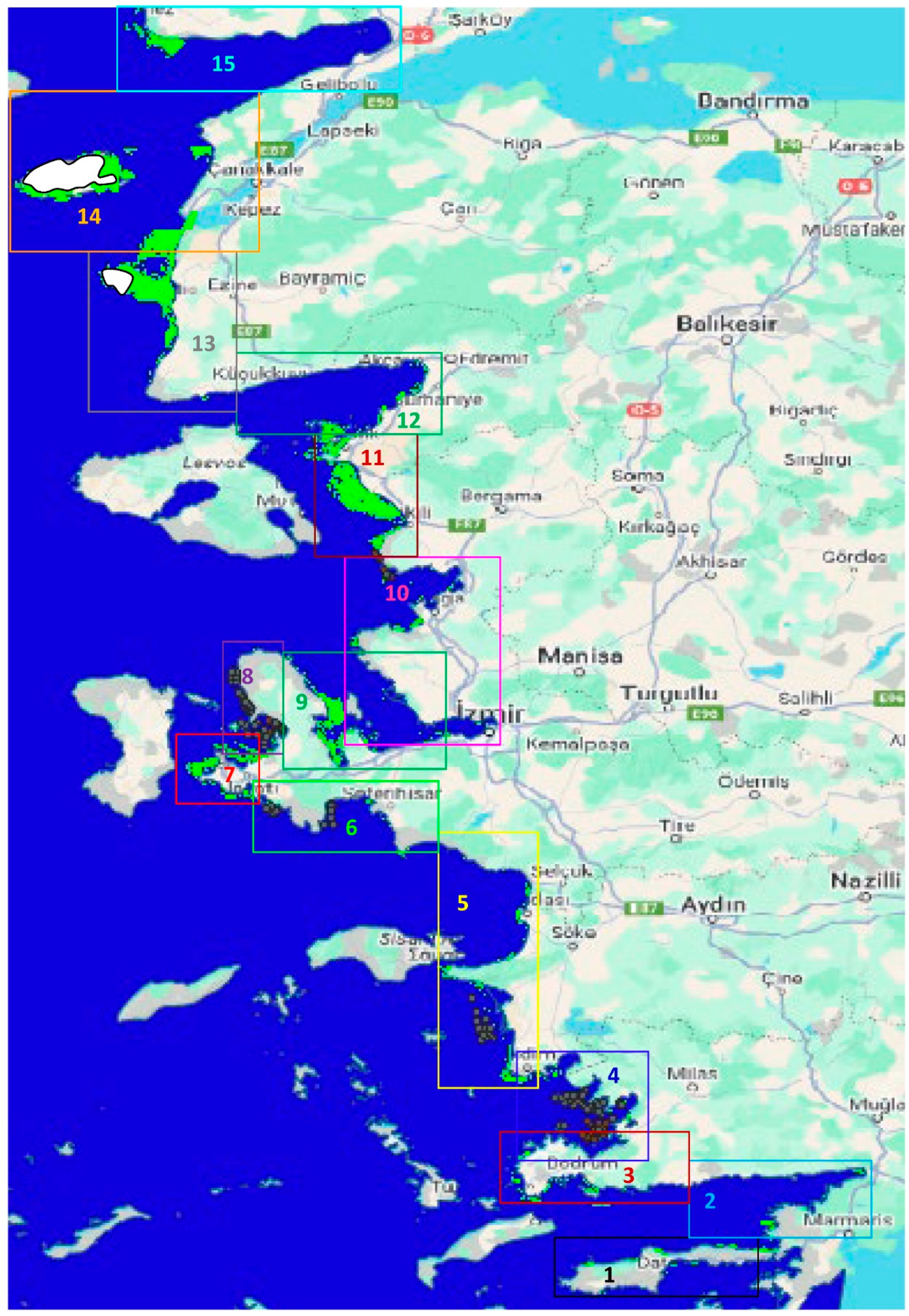
Figure 2.
Corrected bottom depth (m) by PosiBIOM along the study coasts on acoustical tracklines conducted in temporal periods (colors maximally limited one colorbar by 70 m and the greater depths to see detail the shallower water). Arrow shows arrival date and dashed-arrow occurrence near-coastal steep cliffs. Red dashed area shows marine protected area (MPA).
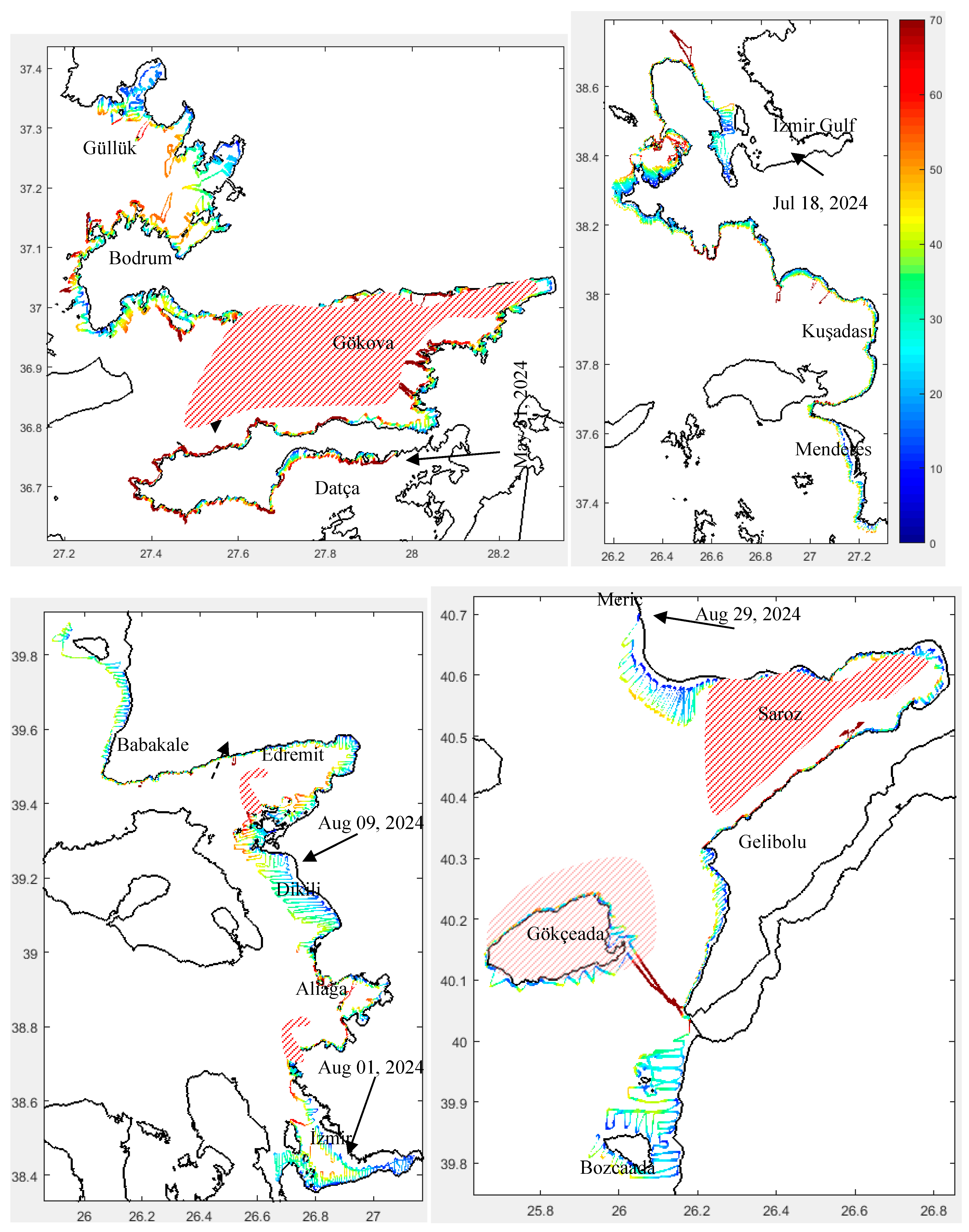
Figure 3.
Monthly averaged surface chlorophyll distribution in a resolution of 4 x 4 km for June, July and August 2024 along the coast of the study area (the maps were provided by Prof. Dr. Ahmet Cemal Saydam from https://oceandata.sci.gsfc.nasa.gov/).
Figure 3.
Monthly averaged surface chlorophyll distribution in a resolution of 4 x 4 km for June, July and August 2024 along the coast of the study area (the maps were provided by Prof. Dr. Ahmet Cemal Saydam from https://oceandata.sci.gsfc.nasa.gov/).
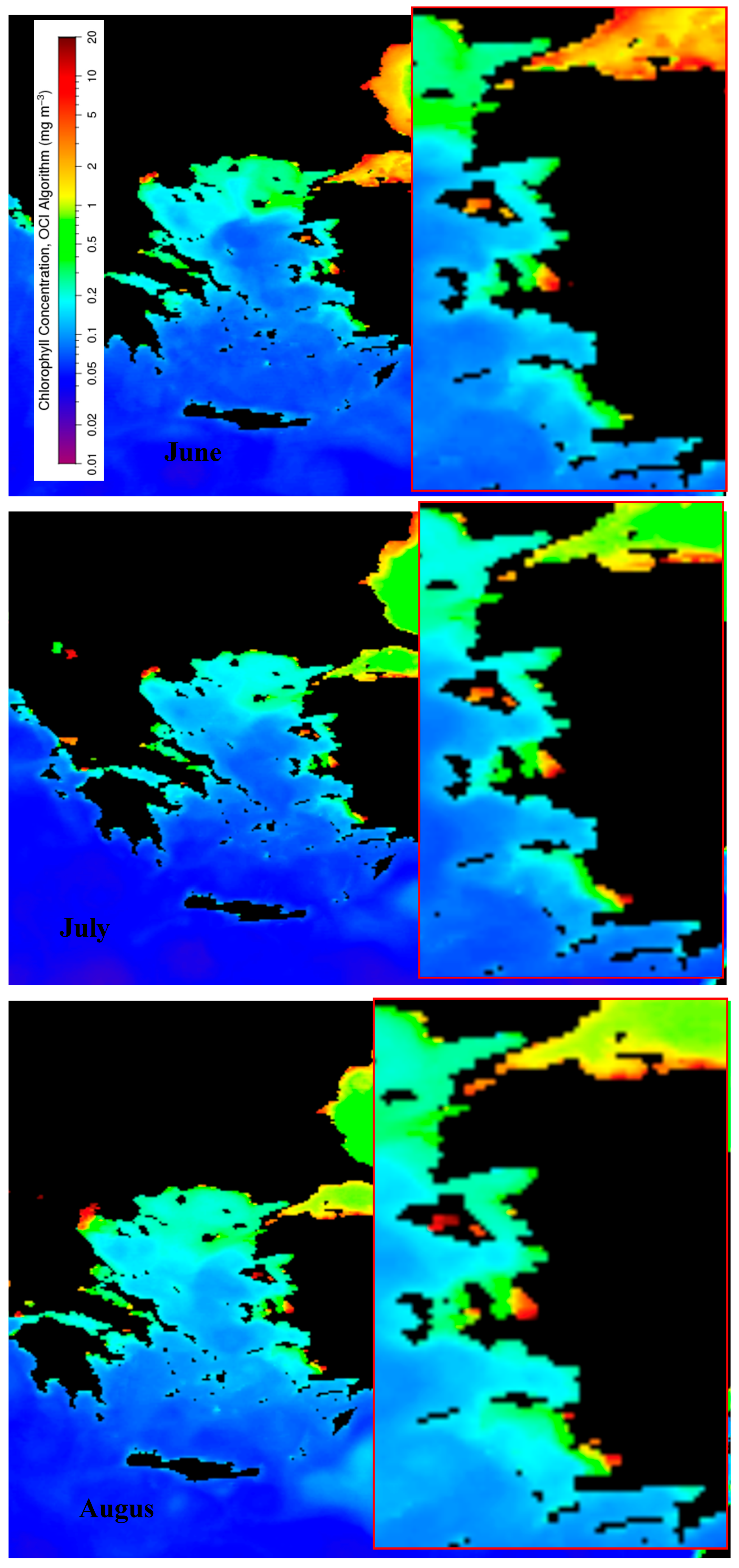
Figure 4.
Sea surface (left panel) and near-bottom (right panel) water temperature in oC (a), salinity in ppt (b), pH (c), dissolved oxygen in mg/l (d), total suspended matter in mg/l (e) and T-S diagram with isoclines of density, σt at the stations colored with geographical latitudes (f) (see Figure. S1 for the station locations) (from [61]).
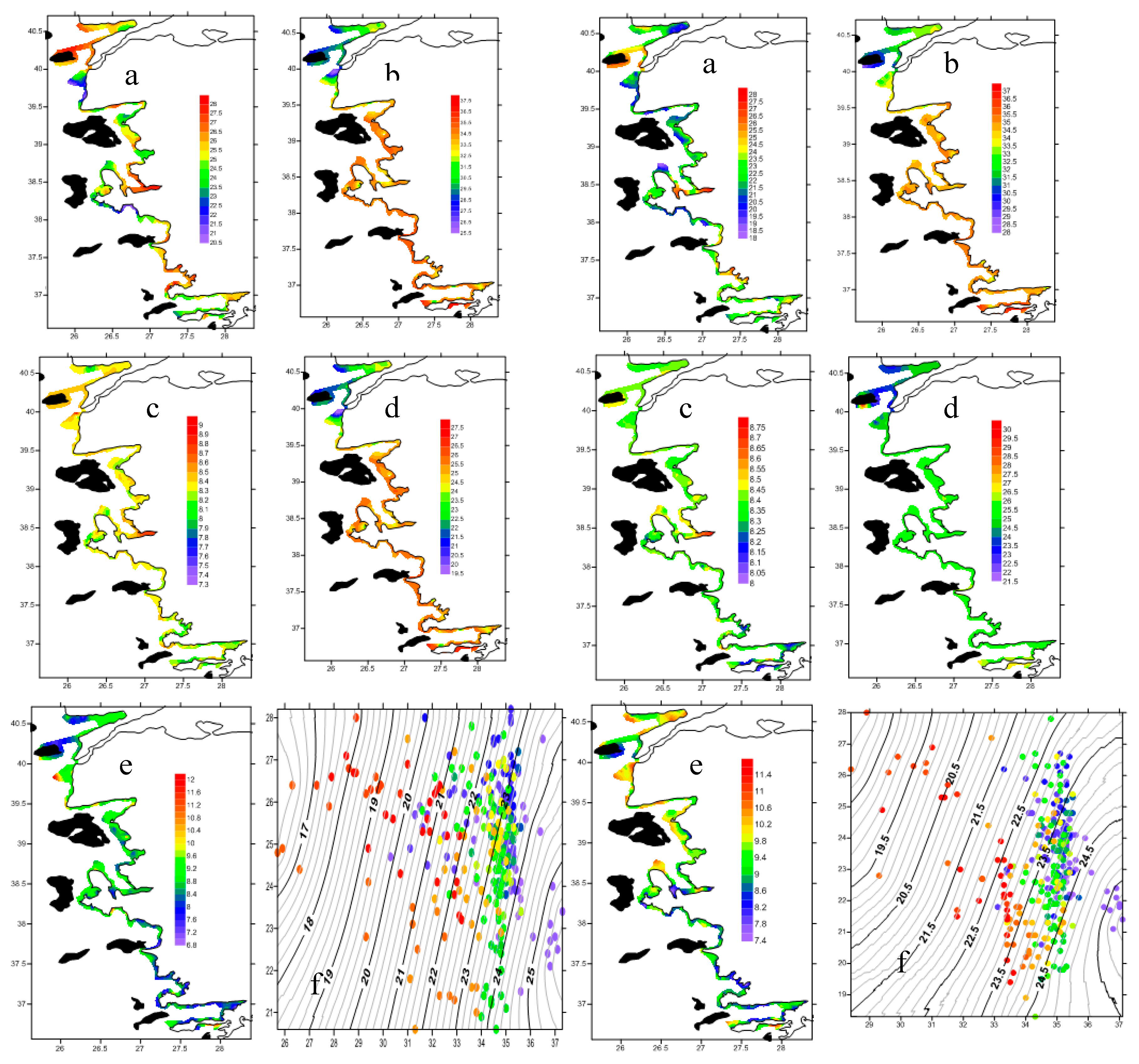
Figure 5.
Secchi disk depth (a) distribution measured in the Aegean Sea study (maximum circle corresponds proportionally to 31.5 m) and the density of the PAR (b) value reaching the bottom measured in the Aegean Sea study (mol photon/cm2/s).
Figure 5.
Secchi disk depth (a) distribution measured in the Aegean Sea study (maximum circle corresponds proportionally to 31.5 m) and the density of the PAR (b) value reaching the bottom measured in the Aegean Sea study (mol photon/cm2/s).
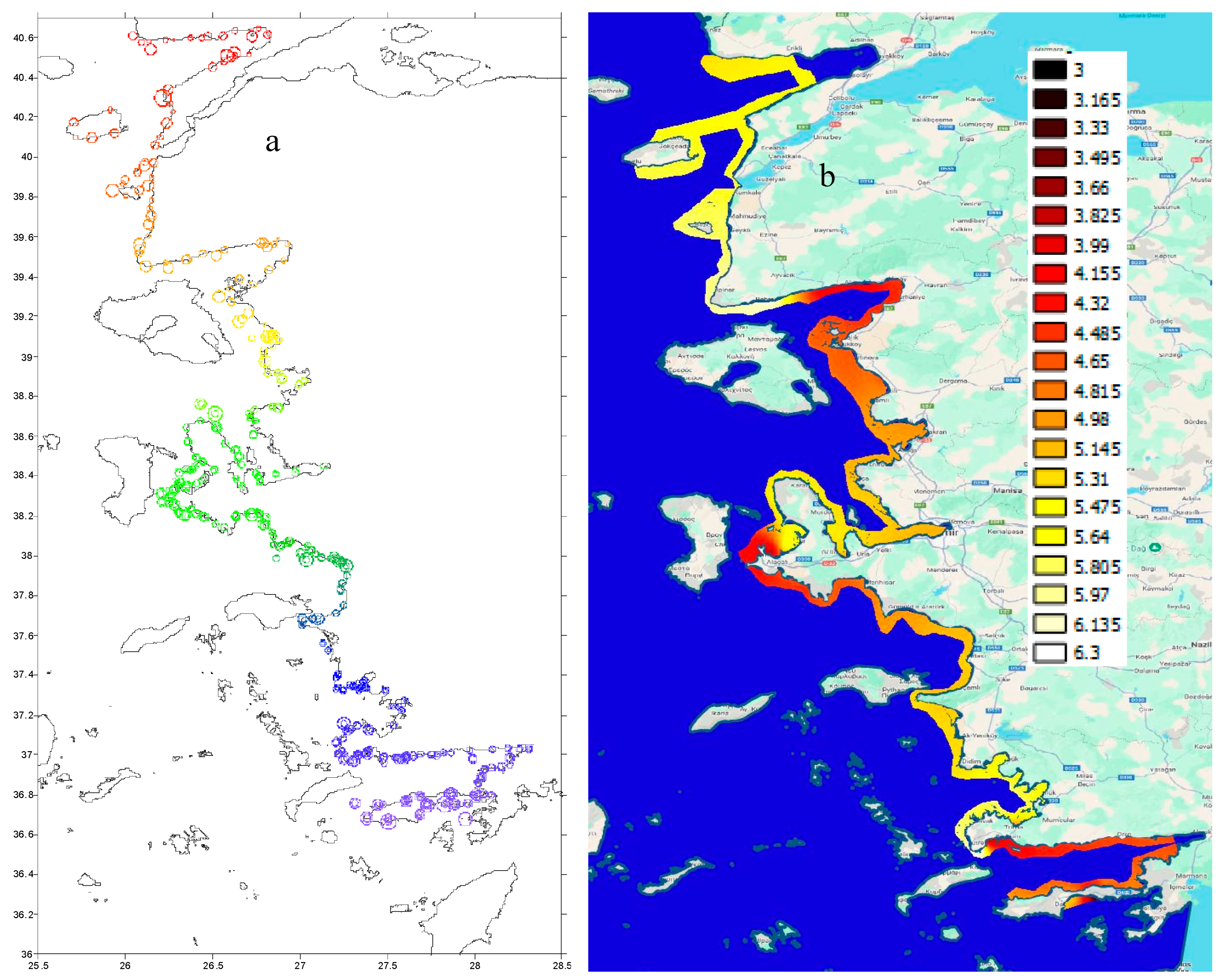
Figure 6.
An example echogram in bottom depth in m vs yearday in format of Julian day.time of hours+min+sec of day (a) with the bottom line (red) and automatic school detection (b) in the corresponding echogram from the beginning in progress, and a variety of school shapes (c) throughout the entire study area from south to north. Each school shape was formed in the direction of left to right headed by the ship and in 2-D of depth (in m on Y-axis) vs horizontal distance (in m on X-axis) converted from the geographical coordinates.
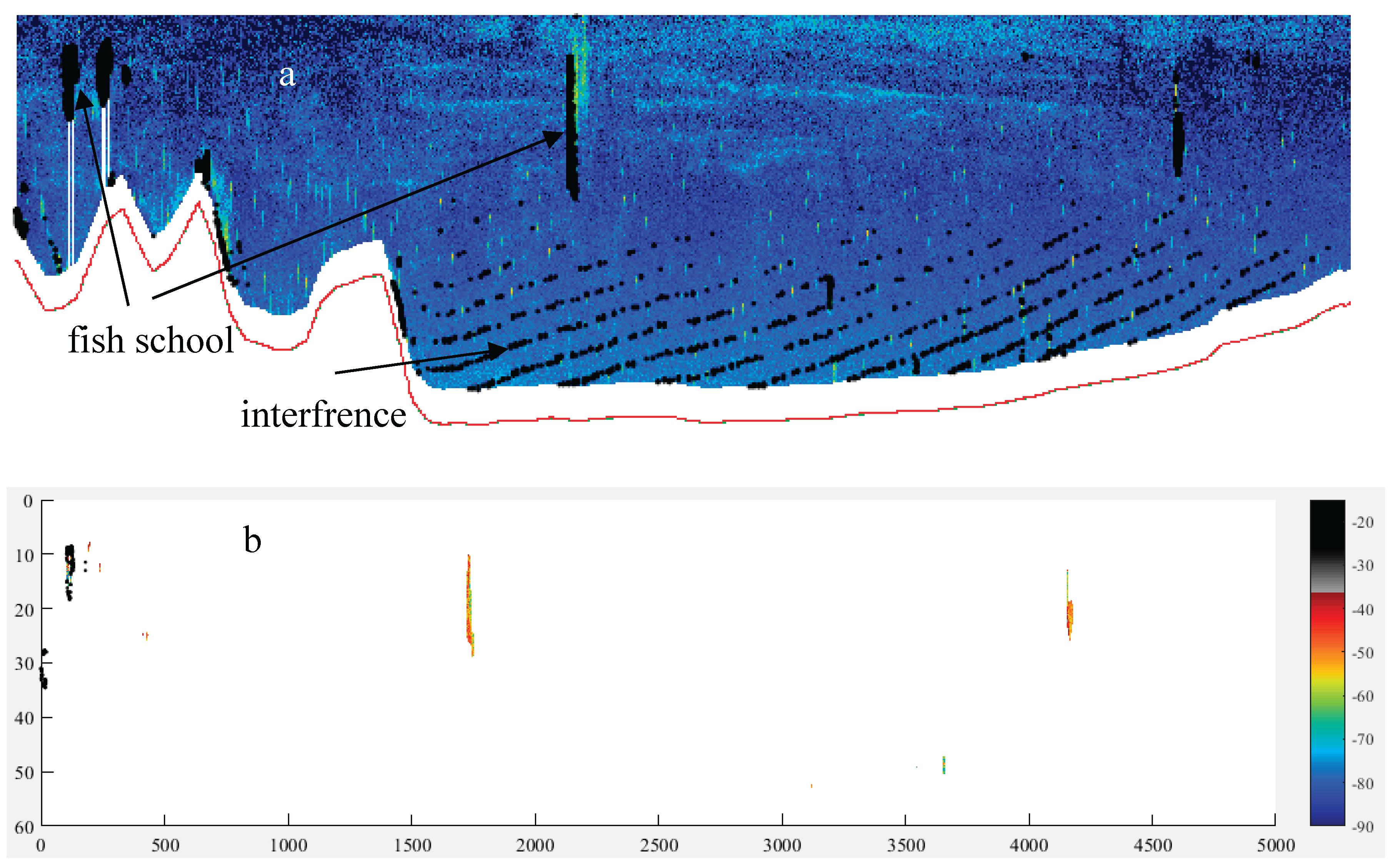
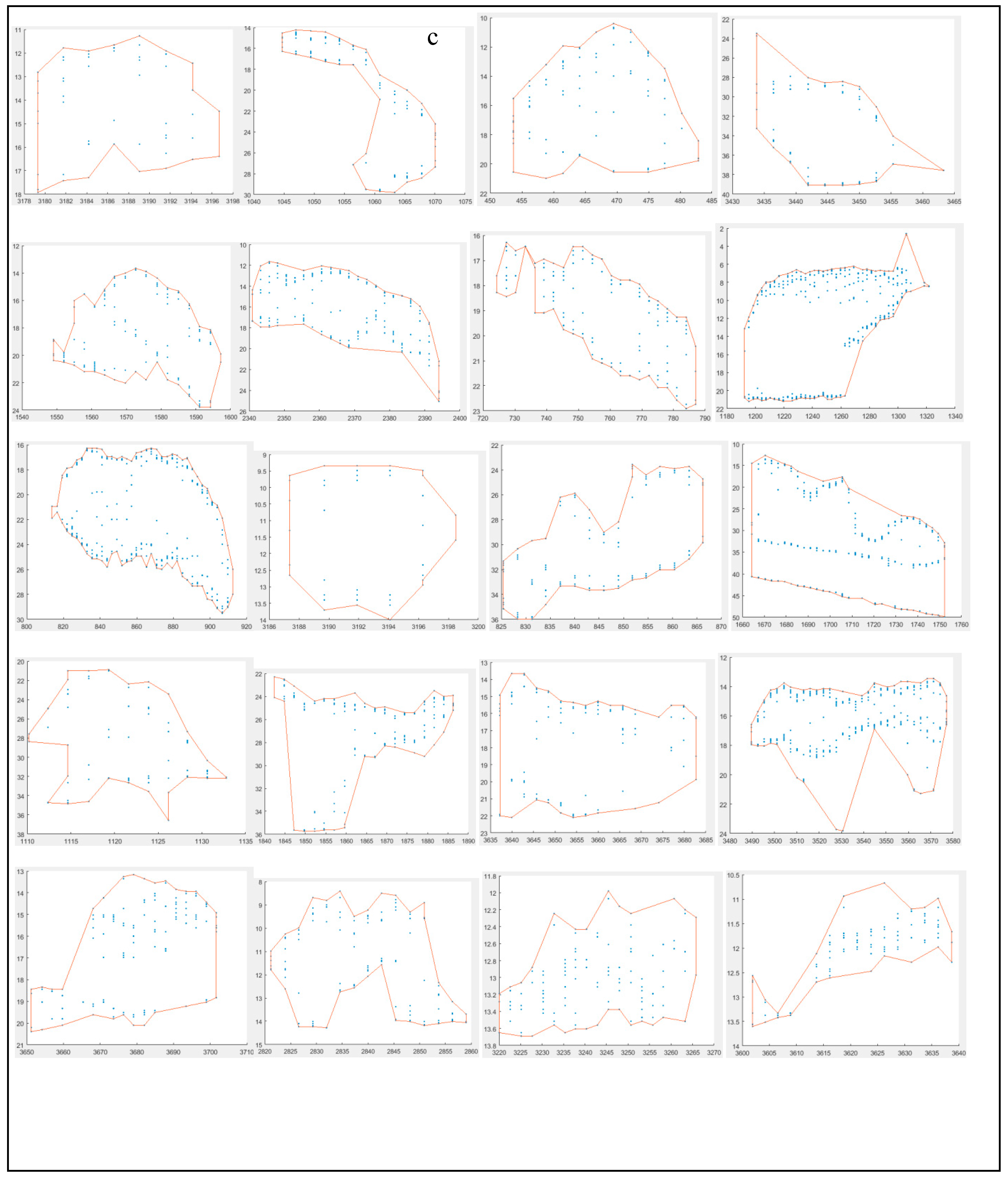
Figure 7.
Spatial distribution of fish school height (m); SH, width (m); SW and vertical area (m2); A along the study area.
Figure 7.
Spatial distribution of fish school height (m); SH, width (m); SW and vertical area (m2); A along the study area.
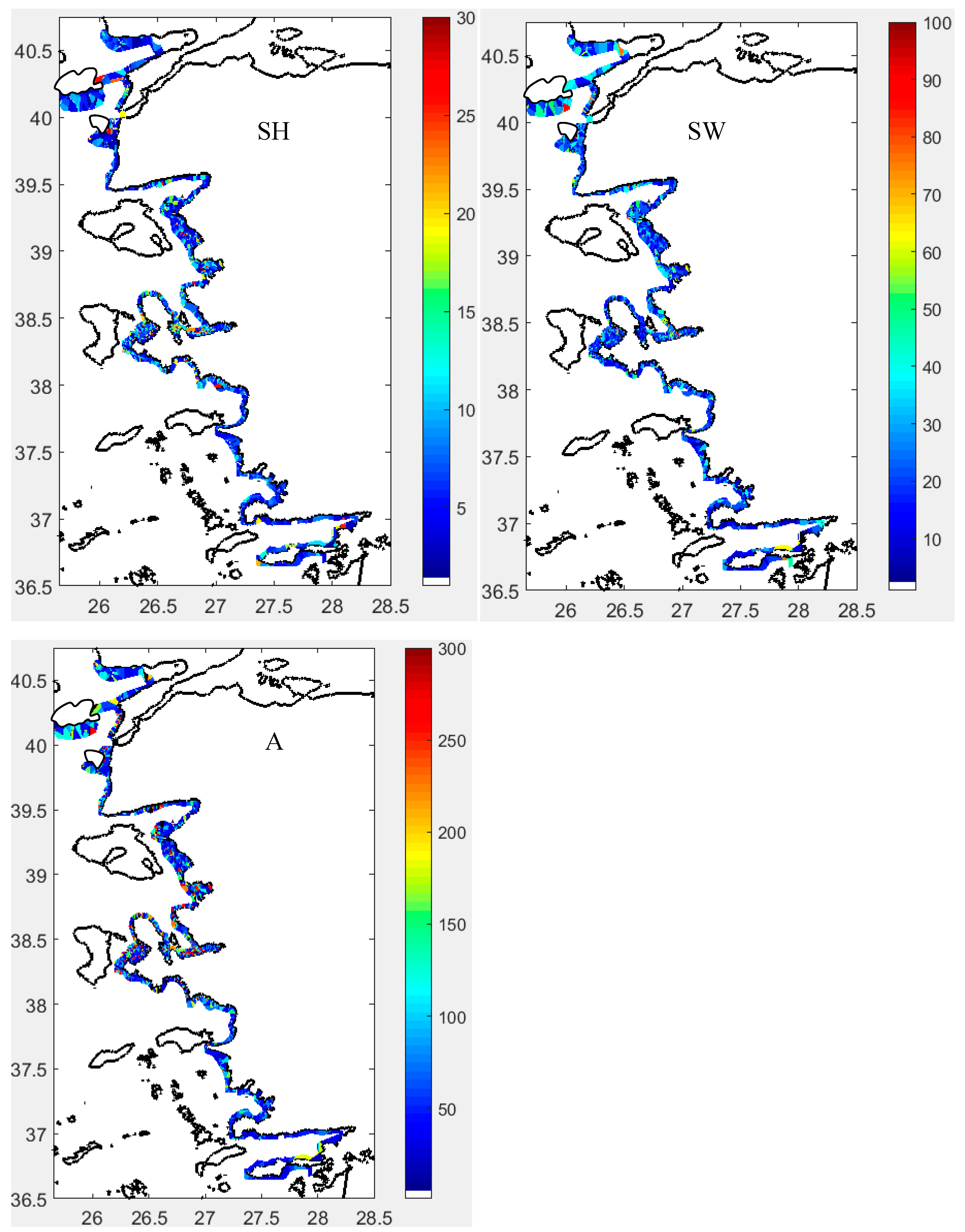
Figure 8.
Spatial distribution of fish school height from the bottom (m); HFB; minimum depth (m); MnD and maximum depth (m); MxD along the study area.
Figure 8.
Spatial distribution of fish school height from the bottom (m); HFB; minimum depth (m); MnD and maximum depth (m); MxD along the study area.
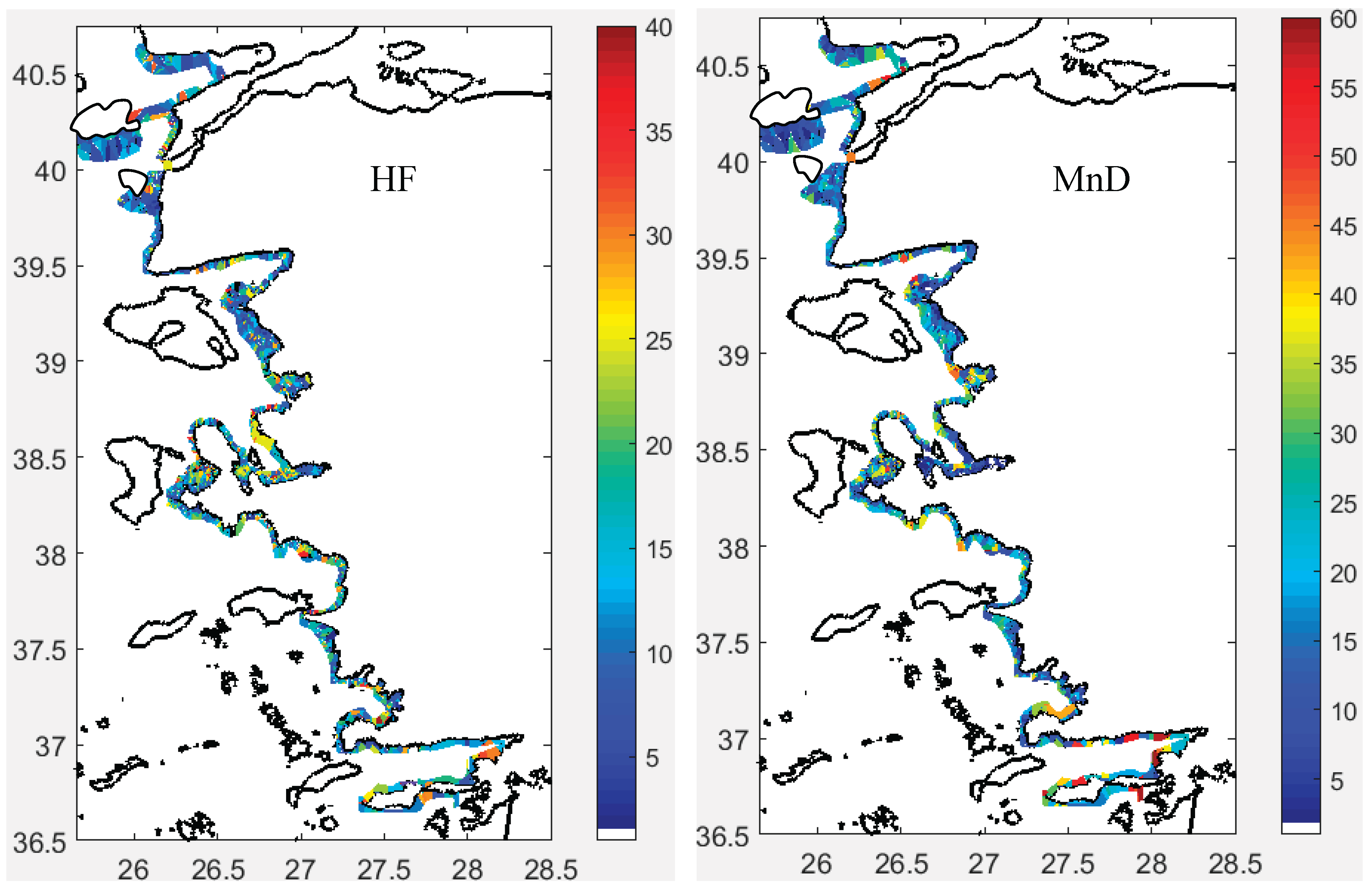
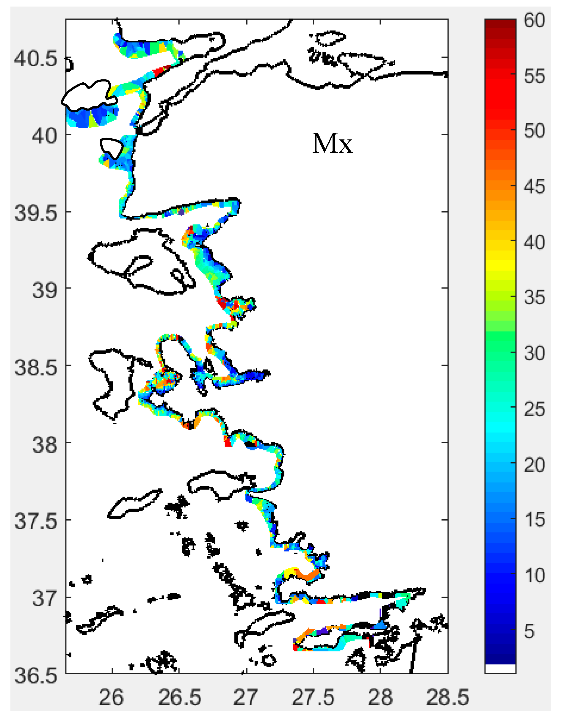
Figure 9.
Spatial distribution of SvE in dB/m3 Sv on edge of fish school, Sv in dB/m3: Sv inside fish school, Sa in dB/m2: backscattering strength of fish school and NASS in dB/nm2: Nautical acoustical scattering strength of fish school.
Figure 9.
Spatial distribution of SvE in dB/m3 Sv on edge of fish school, Sv in dB/m3: Sv inside fish school, Sa in dB/m2: backscattering strength of fish school and NASS in dB/nm2: Nautical acoustical scattering strength of fish school.
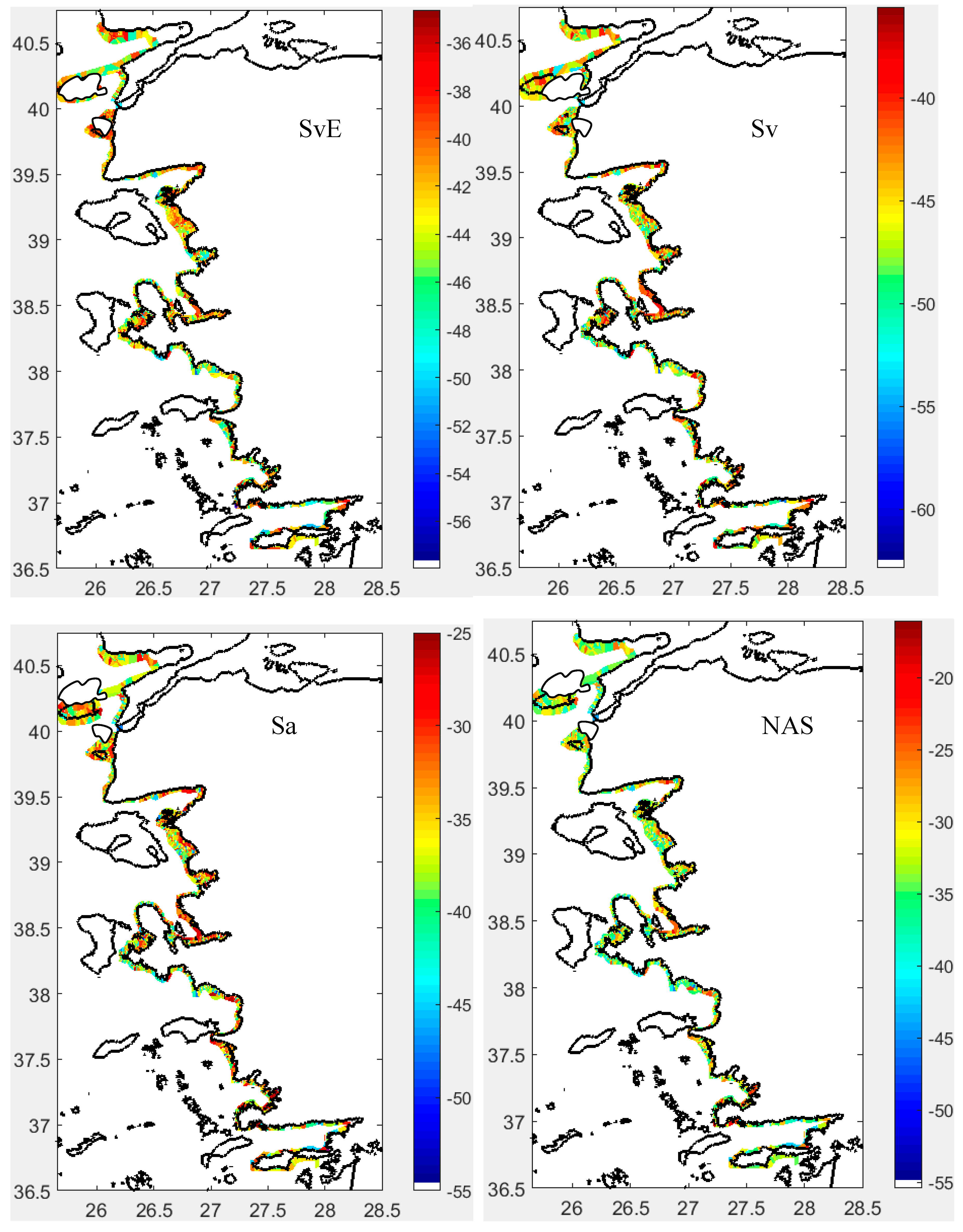
Figure 10.
Optimum number of the clusters estimated by silhouette analysis applied to the data matrix (a), and followed k-means analysis (b).
Figure 10.
Optimum number of the clusters estimated by silhouette analysis applied to the data matrix (a), and followed k-means analysis (b).
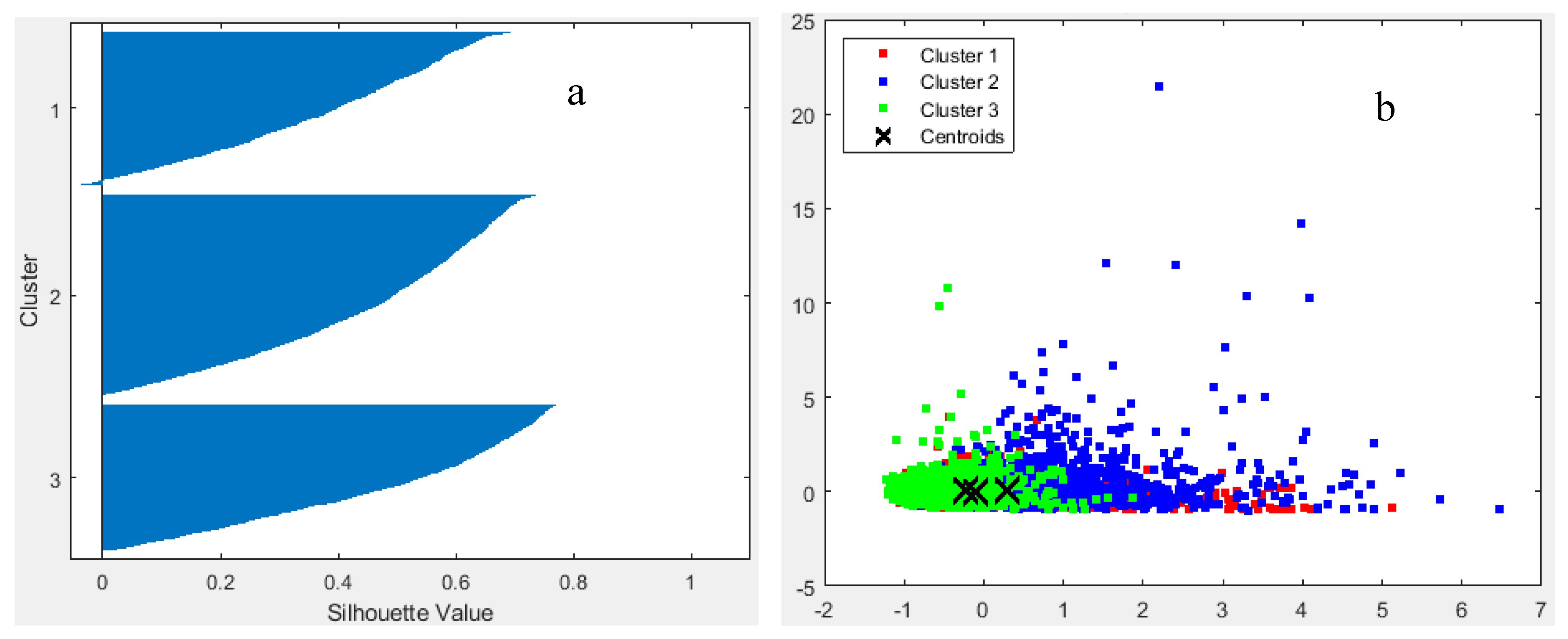
Figure 11.
Spatial distribution of clusters estimated by k-means.
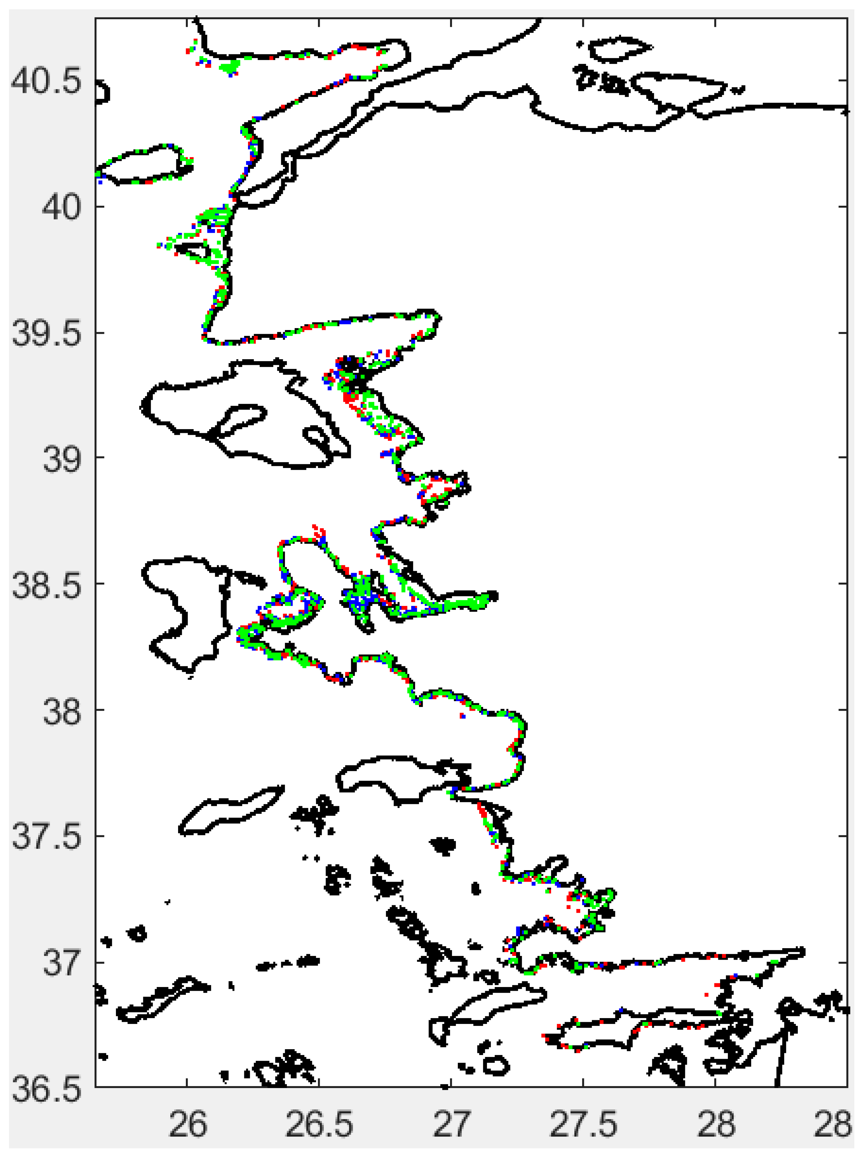
Figure 12.
Co-linearity of the basic morph and acoustical variables for the fish schools classified with number of the clusters estimated by k-means analysis (cluster 1: red, 2: blue, and 3: green, a) and test of the discrimination of the clusters with CAP with cluster number (b).
Figure 12.
Co-linearity of the basic morph and acoustical variables for the fish schools classified with number of the clusters estimated by k-means analysis (cluster 1: red, 2: blue, and 3: green, a) and test of the discrimination of the clusters with CAP with cluster number (b).
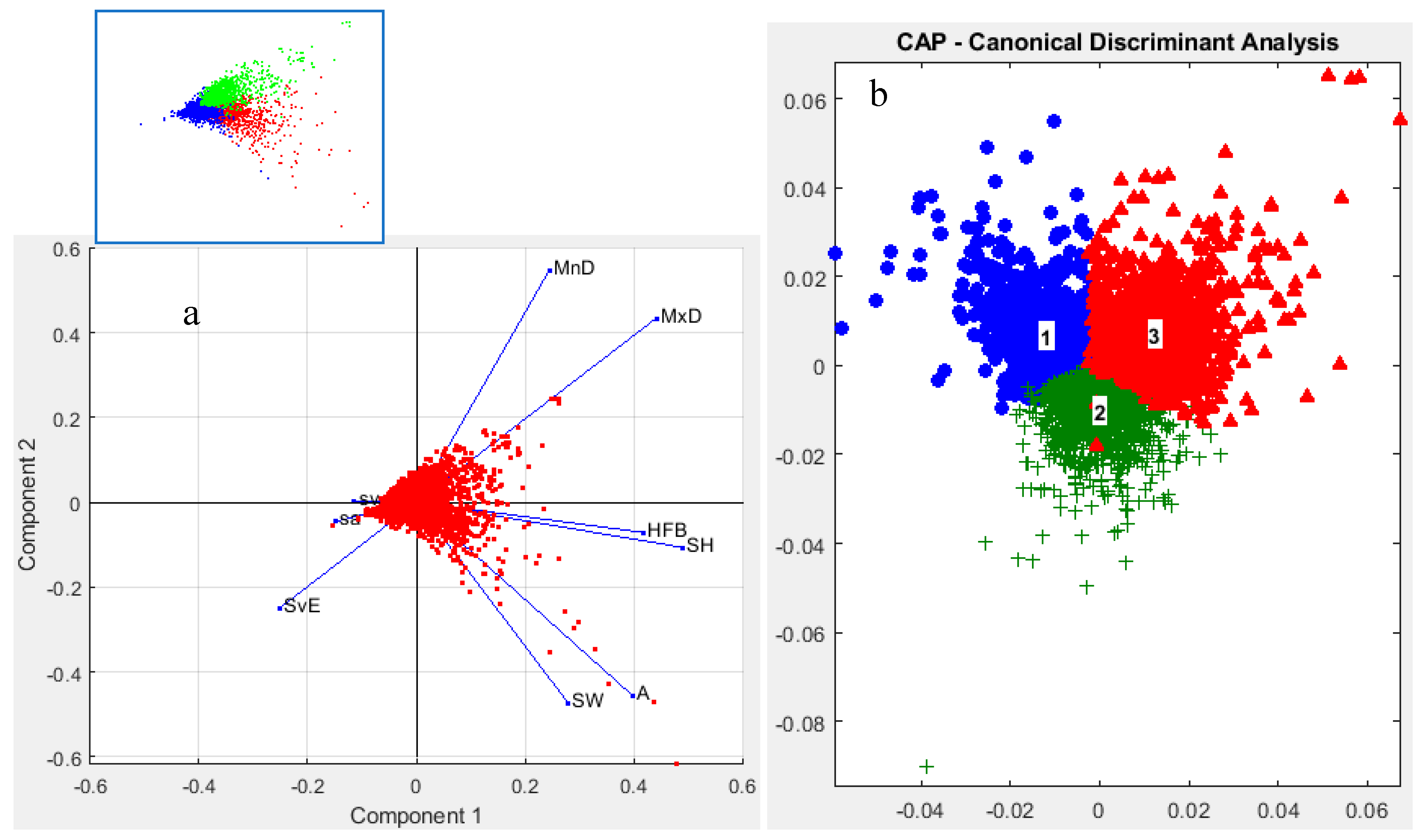
Figure 13.
PCA analysis result, school classified by the bottom depth in different colors, morph and acoustical variables overlapping on configuration of PCA with correspondingly colored circle in scale of each variable strength and the CAP analysis with cluster number (1: 10 m, so on, and 6: ≥80 m).
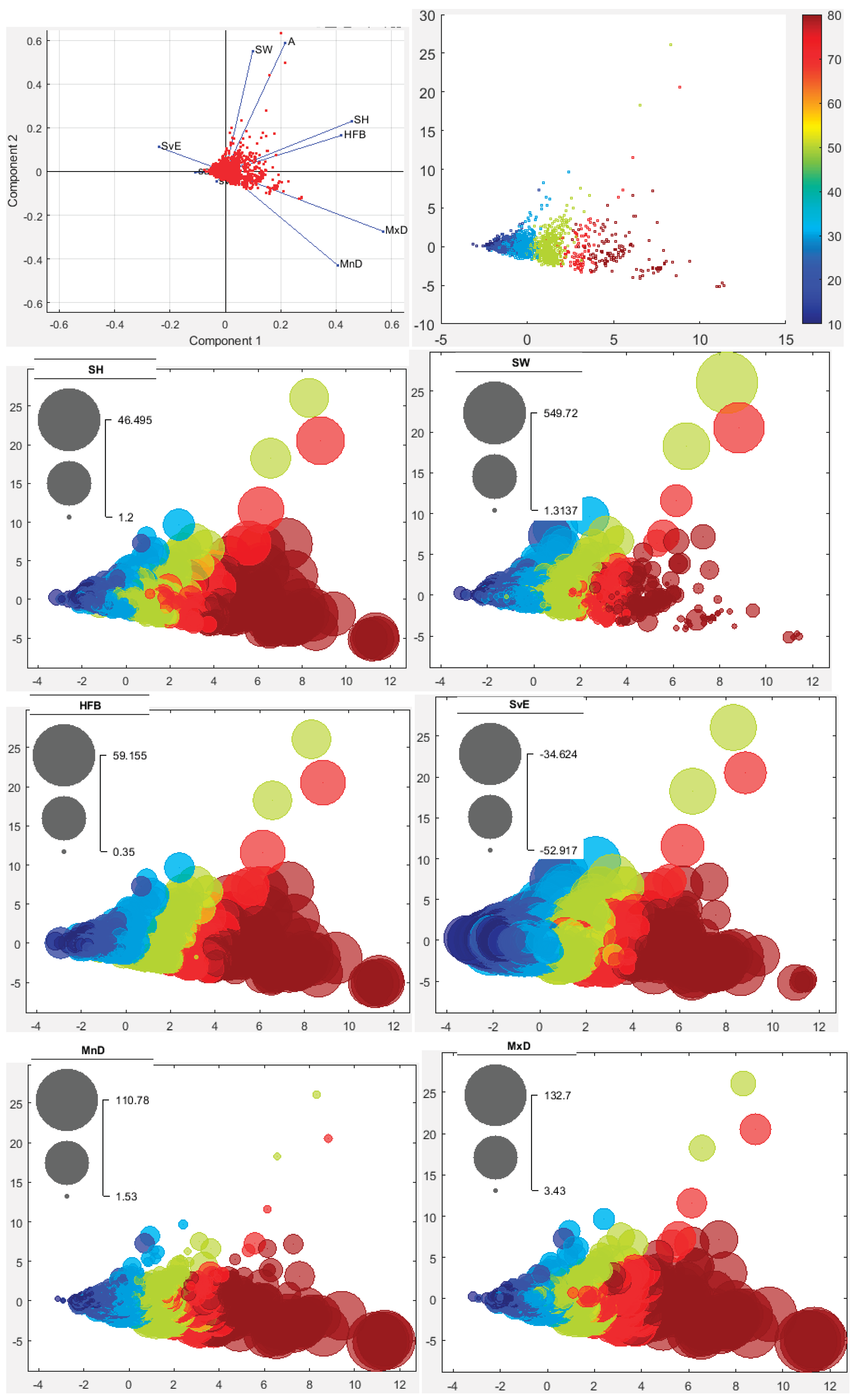
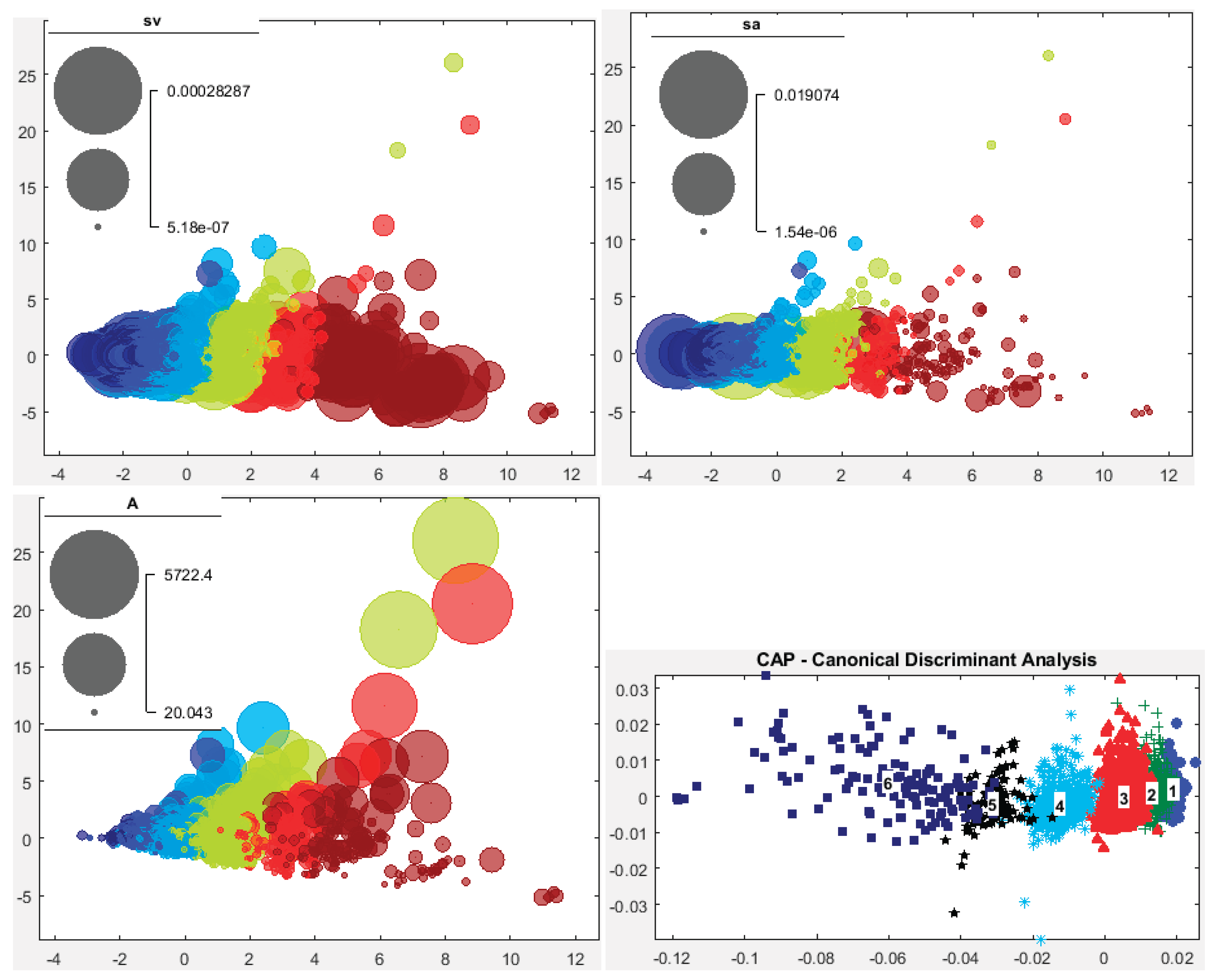

Table 1.
The configuration parameters of the digital echo sounder and settings during the data collection.
Table 1.
The configuration parameters of the digital echo sounder and settings during the data collection.
| Echosounder parameters | Values |
| Manufacturer and model | BioSonics (USA) and DT-X |
| Acoustic frequency | 206 kHz |
| Transducer type and shape | Split and circle |
| Source level | 220.4 dB re µPa at 1 m |
| Receive sensitivity, narrow-beam | -51.0 dB re counts per µPa |
| Receive sensitivity, wide-beam | -56.0 dB re counts per µPa |
| Beam width | 6.8 x 6.8° |
| System noise floor | -140 dB |
| Echosounder settings | |
| Transducer draft | 2.5 m from the surface water |
| Ping rate | 5 pings s-1 |
| Sound speed* | calculated by Visual Acquisition |
| Absorption coefficient* | calculated by Visual Acquisition |
| Data collection threshold | -140 dB |
| Pulse width | 0.1 ms |
| Maximum depth | 70 (200 in cases) m |
*referring the water temperature, salinity and pH.
Table 2.
Score of k-means and possible identical variables for each cluster. Color denote the corresponding each cluster number estimated in Figure. 10b. Cls: cluster and no.
Table 2.
Score of k-means and possible identical variables for each cluster. Color denote the corresponding each cluster number estimated in Figure. 10b. Cls: cluster and no.
| Cls | SH | SW | HFB | SvE | MnD | MxD | sv | sa | A |
| 1 | 0.2983 | 0.0604 | 0.3284 | -0.0707 | -0.28 | -0.1207 | -0.2421 | -0.1077 | 0.1341 |
| 2 | -0.2172 | 0.0362 | -0.2457 | 0.4633 | -0.0938 | -0.2165 | 0.2097 | 0.1214 | -0.0574 |
| 3 | -0.0966 | -0.0825 | -0.1006 | -0.3242 | 0.4735 | 0.3482 | -0.114 | -0.0404 | -0.0636 |
Disclaimer/Publisher’s Note: The statements, opinions and data contained in all publications are solely those of the individual author(s) and contributor(s) and not of MDPI and/or the editor(s). MDPI and/or the editor(s) disclaim responsibility for any injury to people or property resulting from any ideas, methods, instructions or products referred to in the content. |
© 2025 by the authors. Licensee MDPI, Basel, Switzerland. This article is an open access article distributed under the terms and conditions of the Creative Commons Attribution (CC BY) license (http://creativecommons.org/licenses/by/4.0/).
Copyright: This open access article is published under a Creative Commons CC BY 4.0 license, which permit the free download, distribution, and reuse, provided that the author and preprint are cited in any reuse.


