
Submitted:
18 October 2024
Posted:
21 October 2024
You are already at the latest version
Abstract
Bathymetric data is crucial for benthic monitoring in coastal areas but is traditionally obtained through costly and geographically limited acoustic methods. This study uses Satellite-Derived Bathymetry (SDB) in the Eastern Mediterranean, focusing on the Cretan Sea in Greece. It explores how variations in water column optical properties affect SDB models over four years (2019-2022) using Sentinel-2 satellite data. The research covers two areas with contrasting features: Chania Gulf and the open waters around Chrissi Island. Three methodologies were tested: band-ratio, linear-logarithmic, and an inherent optical properties linear model. Significant spatio-temporal variations in SDB models were found due to seasonal changes in water column properties, such as temperature and suspended organic materials. Linear optical properties-based methods performed best, achieving a mean RMSE close to 1 meter, slightly outperforming the ratio-based method. The logarithmic method was less effective, with RMSE values ranging from 1.3 to 1.5 meters. A preliminary Kalman Filter (KF) analysis increased RMSE to the decimeter level. This study demonstrates the impact of water column optical properties on SDB models. It highlights the value of SDB for cost-effective, high-resolution coastal mapping in complex coastlines like those in Greece.
Keywords:
Satellite-derived bathymetry (SDB)
; Water optical properties
; Mediterranean waters
; empirical method
; Kalman filter (KF)
1. Introduction
Seafloor topography, or bathymetry, is vital for various marine activities. Accurate bathymetric maps and data are crucial for navigational safety, helping surface ships, submarines, and remote vehicles avoid underwater hazards and chart safe, efficient routes. Traditionally, bathymetric data has been gathered using shipborne systems with echo sounders and airborne systems with lidar. While these methods are precise, they are also expensive, labor-intensive, and geographically limited, restricting the frequency of surveys. As a complementary approach, Satellite-Derived Bathymetry (SDB) offers additional data in a fast and cost-efficient way, particularly for shallow waters (less than 30 meters deep), by deriving seabed depths from high- to medium-resolution multispectral satellite imagery. SDB enhances them by enabling the mapping of remote and hard-to-reach areas, filling critical gaps in global bathymetric data while at the same time [1].
Advancements in remote sensing technologies have expanded bathymetric research, mainly through high-resolution satellite imagery [2]. Multispectral sensors, especially the green and blue bands, can penetrate up to 25 meters below the sea surface in clear water [3]. The Sentinel-2 MSI sensors, with 10-meter spatial resolution, support bathymetric purposes using freely available datasets. Seafloor topography is dynamic, influenced by natural phenomena like tides, storms, sediment deposition, and human activities such as dredging, fishing, and underwater construction. These changes can be spatial and temporal, making studying spatio-temporal variations in SDB estimates crucial.
The foundational methodology was established in the 1970s [4] and worked in high-transparency waters with a homogeneous bottom. The method differentiates radiances between pixels due to depth differences. Each radiation wavelength penetrates to different depths within the water column and decays exponentially, with the bottom albedo assumed constant [5]. In [3], the satellite spectral bands are considered to have different attenuation rates, requiring minimal calibration data. [6] analyzed optical water properties, needing detailed information on the water column’s optical properties. Tests with a uniform, sand-type bottom showed the method works for any radiation wavelength and water category. Furthermore, the inherent optical properties derived from satellite imagery are used by [7] to estimate SDB, enabling direct analysis without additional sampling.
The study focused on the Eastern Mediterranean, specifically Chrissi Island and Chania Gulf, examining optical properties like absorption, backscattering, and diffuse attenuation coefficients. Greece’s aquatic environment presents both challenges and opportunities for remote sensing bathymetry. With stable year-round conditions and clear waters conducive to SDB. It has the potential to revolutionize hydrographic surveying. SDB’s cost-effectiveness and high-resolution capabilities make it ideal for addressing maritime landscape challenges, from defense and marine trade to scientific research and environmental conservation [8,9].
The Eastern Mediterranean’s unique geological and environmental characteristics further complicate these issues. Factors such as seasonal weather patterns, water characteristics, and human activities can impact the reliability and applicability of SDB estimates. Therefore, a focused study was conducted on the spatio-temporal variations of SDB in this region. This study aimed to understand how variations in water column optical properties affect SDB estimates over time and space. The research addressed several sub-questions, including the impact of seasonal and weather patterns, integrating different satellite-derived products, and choosing satellite image quality and atmospheric correction processors. To achieve these objectives, the study followed a structured approach. It began with downloading seasonal satellite imagery and merging the best images over five years. To ensure high quality, the data underwent rigorous preprocessing, including atmospheric, sunglint, and water column corrections. Bathymetric information was then extracted and compared with ground truth data for validation.
The study extended beyond bathymetric mapping to evaluate water column properties, specifically Inherent Optical Properties (IOPs) and Apparent Optical Properties (AOPs) across seasons. This evaluation helped to understand their influence on SDB estimates and their relevance in hydrographic surveying. Comparative analysis between bathymetry and seasonal variations in IOPs and AOPs provided valuable insights. For future research, data assimilation aimed to refine depth estimations with in-situ measurements. However, additional steps, such as error modelling and algorithm adjustments, are needed.
2. Materials
2.1. Study Area
The study area focuses on Crete Island, located in Greece, which lies in the Southern Aegean Sea, part of the Eastern Mediterranean basin. The island extends approximately between the meridians 23° 28′ E and 26° 21′ E and between the parallels 34° 46′ N and 35° 40′ N. The broader study area is situated on Crete, surrounded by the deepest basin in Greece, with a depth of approximately 2,500 meters in the southern Aegean region. This basin interacts with the Levantine Basin and the Ionian Sea through the eastern and western straits of Crete Island [10].
For SDB estimation, the area is classified into two distinct area of interest (AOI) as seen in Figure 1. The first study area is an embayment of the Cretan Sea located northwest of Crete Island, and it is called Chania Gulf by the name of the local city. It has a length of approximately 22 km, a mean latitude of 35° 33′ N, and a mean longitude of 23° 54′ E. The second study area is located in Chrissi Island, the southeast (SE) part of Crete, approximately 15 km offshore from Ierapetra city, with a mean latitude of 34° 52′ N and a mean longitude of 25° 42′ E.
Generally, the waters are transparent, and the seabed is dominated by sandy substrates with a few rocky outcrops [11]. The west part is included in the NATURA2000 network with the code GR4340003 [12], while the marine part is delimited by the depth curve of 50 m and characterized by the presence of Posidonia oceanica meadows. However, It is noted that the bathymetry increases significantly in the area. Hence, only coastal areas up to 30 m depth are optimal for generating SDB estimates [12]. Additionally, the tidal signal is 15 cm and can be neglected for SDB estimates [8]. The anthropogenic activity is more dominant than Chrissi island because Chania is a well-known tourist destination, with fishing spot areas and sea sports activities conducted from late spring to late autumn.
The typical Mediterranean climate with mild, rainy winters and hot, dry summers characterizes Crete island. The atmosphere can be quite humid, depending on the proximity to the sea, while winter is relatively mild [11]. The complex ocean circulation patterns and water mass interactions can result in localized areas of higher nutrient concentrations, especially in upwelling zones or regions with vigorous vertical mixing [10]. The study areas were selected mainly because of the profound water clarity and secondly because of the diametrically opposite location concerning the AOI. Chania Gulf is a more enclosed area of Crete Island, while Chrissi Island is in open seas. Hence, investigating SDB estimates under different hydrodynamic conditions can produce significant insights for the Eastern Mediterranean.
2.2. Satellite Data
Sentinel mission products are freely available for download via the Copernicus Open Access Hub. This study used Level-1C raw satellite imagery to extract water optical properties, utilizing adjustable atmospheric correction parameters. As indicated in Table 1, the imagery spanning from 2019 to 2022 was filtered by month and limited to 2% or less cloud coverage. The selected period aligns with recent in-situ measurements and was extended by five years to capture significant bathymetry changes. Additionally, Sun-Zenith Angle (SZA) products above 70° were excluded to reduce solar reflection [13].
2.3. Field Data
In empirical SDB estimation used in this study, field data were used to calibrate and validate the SDB models. For Chrissi Island, ground truth data came from the Hellenic Navy Hydrographic Service’s Electronic Navigational Chart (ENC) GR3CFDES (scale 1:90,000), last updated on 23 February 2022, with depths referenced to the Low Astronomical Tide (LAT). For Chania Gulf, the Hellenic Center for Marine Research collected data during bathymetric surveys from January 2014 to May 2015. Instruments included a Humminbird Single Beam Echo Sounder (SBES) and a Reson 7125 dual-head Multibeam Echo Sounder (MBES). Positioning errors were reduced using a Real-Time Kinematic (RTK) solution from the Hellenic Positioning System (HEPOS), with depth corrections applied for LAT and the sensor’s draught [11].
3. Methods
3.1. Empirical Satellite-Derived Bathymetry (SDB)
In the current study, the SDB models under investigation are the linear-logarithmic algorithm proposed by [4], the band-ratio transformation developed by [3], and the inherent optical properties linear model (IOPLM) proposed by [7]. Lyzenga developed a method for studying marine environments with low suspended particles, chlorophyll, and organic matter levels. This method assumes that the physical and chemical properties of the water column depicted in a satellite image remain consistent. The ratio of attenuation coefficients due to light diffusion in two spectral zones should remain constant across the entire image [14]. However, this assumption may only hold in some cases, as reflectances from the water bottom may vary depending on the sediment composition.
One spectral band’s use for deriving depth estimates is primarily based on the reflectivity of the seabed, also known as albedo. If the reflectivity of the seafloor decreases, it can lead to an overestimation of the sea depth. However, shortly after, the same researcher discovered that analyzing two spectral bands can account for the variability of the seafloor’s reflectivity [14]. This results in a more precise estimation of depth, which can be calculated using the following equation:
where is the water leaving reflectance, is the reflectance of the optically deep water areas of the image, , , are the multiple regression analysis coefficients and z the estimated water depth.
A significant disadvantage of the linear-logarithmic algorithm in coastal environments consisting of underwater vegetation, such as algae or seagrass, is that the bottom reflectance in shallow water is lower than that in deep water . As a result, in shallower waters, the difference is smaller than zero, thus the natural logarithm is not defined. The different spectral zones of passive sensors exhibit distinct spectral absorptions (attenuations), and the depth values in the Lyzenga equation vary as a function of the logarithm; therefore, the ratio of the logarithms, for example, between blue and green bands, will also change according to the depth.
A variation in the bottom albedo, caused by changes in underwater vegetation or sediment, affects both spectral zones similarly, while changes in depth significantly impact the zone with higher absorption. Thus, the variation in the reflectance ratio between spectral zones due to depth will be much more significant than the variation caused by changes in bottom quality [15]. Consequently, when investigating a coastal area with a constant depth but different bottom compositions, satellite imagery pixels displaying varying reflectance due to sediment and vegetation will have a nearly consistent logarithmic reflectance ratio. Hereafter, a ratio transform algorithm to determine the bottom depth is proposed by [3], regardless of the bottom quality or existing vegetation. It can be calibrated to actual depths using data from a nautical chart or a bathymetric plot or through field measurements using the following mathematical formula:
where is an adjustable constant, which serves to tune the ratio to the depth of the chart or filed measurements, n is a constant that is associated with the area of interest, and m_0 is an offset constant for the depth that corresponds to 0 m (z=0). It should be noted that the constant n is chosen to ensure that the logarithm is always positive, so the ratio produces linear or proportional results as a function of the change in depth. In addition, the coefficients and can be determined by statistically correlating the reflectance values and field data at the corresponding pixel positions.
The last SDB method tested in this study is based on the IOPs and their fluctuations with depth; thus, the IOPLM was developed by [7]. This model utilizes the blue and green bands from WorldView-2 multispectral images, which offer very high resolution, to gather a wide range of water depth data. The formula consists of the following components:
where and are the regression coefficients; and are the inherent optical parameters of the blue band (i) and the green band (j), related to the absorption and backscattering coefficient. Finally, z is the depth estimation. The inherent optical property parameter u can be calculated after Equation 4.
Here, and are model constants that change with various water optical properties. Their values may vary with the particle phase function and differ from ocean to coastal waters. To be applied to both coastal and open water bodies, [6] use the averaged values = 0.0895 and = 0.1247 to develop the multiband quasi-analytical algorithm (QAA). This algorithm aimed to retrieve the absorption and backscattering coefficients from remote sensing reflectances of optically deep waters. Because “u” is just a ratio of the backscattering coefficient to the sum of absorption and backscattering coefficients, knowledge of the absorption coefficient enables estimating the backscattering coefficient and vice versa.
In addition, is the subsurface remote sensing reflectance. It can be obtained by the conversion of the atmospherically corrected reflectance Rrs (λ) [16], as follows:
To summarise the steps of the last method, one has to start by calculating the subsurface reflectances from the atmospherically corrected remote sensing reflectances for both the green and blue bands. Then, derive the inherent optical parameter “u” from Equation 5 for both blue and green bands. Finally, the ratio of the “u” parameter between the two bands has to be plotted (scatter plot) against the field measurements, and after regression analysis, the regression coefficients are deduced. This linear equation is the SDB estimation for the scene of interest.
In addition, the SDB estimations for the summer period following the C2RCC atmospheric processor were also subjected to this process. On the contrary, the ACOLITE processor calculates the water optical parameters automatically using QAA [6], and the user should implement the last step of regression analysis and calculate the linear response equation. An important note is that this IOPLM method was initially developed for very high spatial resolution (~ 2 m) satellites such as WV-2, SPOT, and Pleiades. In this study, the Sentinel-2 products belong to the high spatial resolution, and all the tests were executed with the best value of 10 m of visible bands.
In conclusion, two factors primarily influenced the selection of the three methodologies mentioned above for remote sensing bathymetric derivation. Firstly, these methodologies are based on distinct principles and utilize different techniques for depth estimation, thus providing a diverse and comprehensive approach. Secondly, they offer varying approaches to the relationship with the water’s optical properties, a crucial aspect of this research. Within this context, the linear transformation technique does not accommodate variations in the water’s optical properties, operating under the assumption of a homogeneous water column throughout the testing period. Conversely, the other two methodologies integrate the variability of the water’s optical properties into their computation, providing a more dynamic representation of the aquatic environment.
The technique of band ratio transformation accommodates the oscillations in the water’s optical properties indirectly by measuring the actual responses of the spectral bands, which encapsulate the influence of these optical properties. Conversely, the IOPLM method operates on a more direct principle. It is grounded on the inherent optical parameter ‘u’, which explicitly incorporates the responses associated with absorption and scattering phenomena within the water column.
3.2. Kalman Filter (KF) Smoothing
The Kalman Filter is an algorithm used to estimate the state of a linear dynamic system in the presence of uncertainty and noise. It operates through two main steps: prediction and update. In the prediction step, the filter estimates the system’s next state based on the current state and control inputs [17]. The filter utilized in this study uses the field data as the initial state. In contrast, the SDB estimates is used as the measurement input for updating the bathymetry model, as notated in Equation 6 to Equation 10.
The filtering involves calculating the predicted state estimate using the state transition model and any control inputs , and predicting the estimate’s uncertainty by considering both the previous uncertainty and process noise . The update step refines this prediction by incorporating new measurements. The Kalman Gain is calculated to determine how much the new measurement should influence the updated state estimate. The updated state estimate then, the Kalman Gain moderates this correction based on the difference between the predicted and actual measurements. Finally, the estimated covariance is updated to reflect the reduced uncertainty after incorporating the measurement.
Through these iterative prediction and update steps, the Kalman Filter continuously refines the state estimate, providing a more accurate and reliable estimate of the system’s state over time, even in noise and uncertainty. The KF can be further refined and optimized based on the specific characteristics of the data, the research objectives, and the use of an iterative KF to model the error and reformulate the SDB equations
3.3. Water Optical Properties
Ocean color is influenced by its optical properties, which are categorized into Inherent Optical Properties (IOPs) and Apparent Optical Properties (AOPs) [18]. IOPs depend only on the medium (seawater) and are not affected by external factors. Key IOPs include absorption, where light energy is converted to heat or chemical energy, and scattering, where light changes direction or wavelength [19]. AOPs are influenced by both the IOPs and the geometry of light propagation. AOPs include reflectance and diffuse attenuation coefficients, which describe how light is scattered or absorbed through water [20].
IOPs and AOPs are connected through the Radiative Transfer Theory (RTE), where IOPs are used to calculate radiance, from which AOPs are derived. In remote sensing, inversion techniques are employed to estimate water column properties like bio-optical parameters and seafloor depth from known radiance values [19,21]. Beyond the inversion techniques mentioned above, alternative, more empirical methods exist to assess the radiation propagation state within a specific water column and remove the additive haze effect sourced from scattering. One such method is Dark Object Subtraction (DOS), initially proposed by [22]. This technique is employed under the assumption that in deep-water regions, any radiation reflected from the seabed is virtually absent due to high absorption levels. Consequently, the sensor’s reflectance recordings in these regions are attributed solely to sources other than the bottom substrate. By subtracting the deep-water pixel values from the pixel values across the entire imagery, it is posited that what remains is essentially the bottom reflectance.
In conclusion, the water column’s inherent and apparent optical properties are pivotal in determining the precision and dependability of Satellite-Derived Bathymetry. These optical characteristics present both obstacles and avenues for methodological enhancements. Although factors such as water clarity, absorption, and scattering coefficients may impose constraints, the advancement in understanding their impacts and integrating corrective measures has contributed to the ongoing refinement of accurate and robust SDB algorithms. For satellite observations, the reflectance signal (Rrs) is a mix of water-leaving signals and sunlight reflected off the water surface (sunglint). Proper sunglint removal is critical, as ignoring it can lead to significant errors in depth estimation [23]. The method by [19] was used for sunglint correction, which applies linear regression between near-infrared (NIR) and visible bands to estimate and remove sunglint from visible wavelengths.
3.3. Workflow
Despite the multitude of Satellite-Derived Bathymetry models available for bathymetry estimate extraction, preprocessing is nearly ubiquitous across all techniques. The preliminary steps for SDB analysis include atmospheric correction for Level-1C products, image resampling, clipping the imagery to correspond with the study region, and application of a sea-land mask using the NIR band (B8) of Sentinel-2A to spot marine features. After these preprocessing stages, the comprehensive methodology implemented in this study is presented in the workflow chart in Figure 2.
The Sentinel-2 mission provides 13 spectral bands, covering the visible near-infrared (VNIR) and short-wave infrared (SWIR) regions. Three visible bands—red (R), green (G), and blue (B)—with a spatial resolution of 10 meters are essential for generating Satellite-Derived Bathymetry (SDB) estimates. However, Sentinel-2’s multispectral bands vary in resolution, necessitating an initial resampling step to ensure uniformity across all bands. To improve bathymetry accuracy, this study adjusted all bands to the highest possible spatial resolution (10 meters). A subset of Sentinel-2 Level-1C images, covering approximately 100 square kilometers with a 10-meter resolution, focused on the area of interest (AOI). An RGB image confirmed the AOI and a land cover mask was applied to highlight marine features. Using the NIR band, land areas were masked out based on a threshold or polygon, isolating aquatic regions. Following the method by [24], a linear regression between the NIR and visible bands was applied to adjust pixel values and emphasize marine areas. Atmospheric corrections were made using the Dark Object Subtraction (DOS) method to correct for atmospheric scattering.
Two atmospheric correction (AC) processors, ACOLITE DSF and Case 2 Regional CoastColour (C2RCC), were employed. ACOLITE, developed by the Royal Belgian Institute of Natural Science (RBINS), is used for aquatic applications on satellites like Sentinel-2 and Landsat [26]. Its Dark Spectrum Fitting (DSF) algorithm estimates atmospheric path reflectance by using multiple dark targets in the scene to determine the best-fitting aerosol model [27]. C2RCC, an ocean color processor with multi-mission capabilities, works by inverting radiative transfer simulations through neural networks, applying an IOP model to retrieve water properties [28]. ACOLITE DSF also includes sunglint correction, which estimates sunglint using SWIR bands and applies it to VNIR bands [29]. This process requires prior knowledge of aerosol optical properties from in-situ measurements or the Copernicus Atmospheric Monitoring Service (CAMS) model [30].
The DOS method assumes that dark objects in the image contain significant atmospheric scattering, and this atmospheric offset is subtracted from each pixel [22]. The best target for DOS is water with zero reflectance [31]. ACOLITE DSF automatically removes negative reflectances to avoid outliers. The study analyzed band response to light attenuation using the logarithmic-linear band model [4], band-ratio transformation [3], and IOP model [7]. The processors use nonlinear least squares to compute key IOPs, including absorption and backscattering coefficients, turbidity, and suspended particulate matter (SPM) concentrations [32,33]. Chlorophyll-a (Chl-a) concentration was calculated using the blue/green ratio algorithm in the ACOLITE DSF processor. C2RCC also provided chlorophyll-a estimates, helping understand biological activity and seasonal variations in water properties influenced by river runoff, water mixing, salinity, and temperature [28].
Several error metrics were used to evaluate the accuracy of SDB estimates. The Root Mean Square Error (RMSE) measures prediction accuracy, with lower values indicating closer alignment between satellite-derived depths and field measurements [34]. The Mean Absolute Error (MAE) quantifies the average magnitude of errors without regard to direction, while the Median Absolute Error (MedAE) provides a more robust measure against outliers [35]. The Mean Absolute Percentage Error (MAPE) expresses errors as a percentage, which is useful for comparing performance across different datasets [36]. These discrepancies in in-depth estimates were compared to the S-44 Ed. 6 Standard predictions for the total vertical uncertainty (TVU) associated with a Special Order survey [37]. Lower values across these metrics suggest more accurate depth estimations, indicating the effectiveness of this study’s applied atmospheric correction and SDB methods.
4. Results and Discussion
4.2. Water Optical Properties Analysis
The diffuse attenuation, absorption, and backscattering coefficient describe the water optical properties for both study areas. The breakdown of these coefficients shows a similar pattern for both study areas, as seen in Figure 1. Overall, the diffuse attenuation coefficient describes how rapidly light diminishes with depth. A higher value indicates that light diminishes faster, suggesting murkier waters, while a lower suggests more transparent waters. Hence, it shows a general decrease for winter datasets as depth increases. This indicates that waters tend to be more apparent in deeper parts. The higher values near the surface indicate particle concentration. Like winter, the values decrease with depth during spring. This pattern suggests that the surface waters are relatively murkier, and clarity increases with depth. The change from winter to spring might be less pronounced, but the general trend of more transparent waters at depth remains consistent.
Afterward, the absorption represents the fraction of light absorbed by substances in the water, such as dissolved organic matter, phytoplankton, and detritus. A higher absorption coefficient suggests that more light is absorbed, decreasing water clarity, while a lower value suggests more transparent water. During winter, the absorption values of all bands generally decrease with depth; thus, this trend indicates that the amount of absorbing substances (like phytoplankton or dissolved organic matter) is higher near the surface and decreases at deeper parts.
Similarly, the backscattering coefficient indicates the amount of incident light scattered back out of the water. A higher value implies more particles that scatter light, while a lower value means more transparent water. Concerning winter datasets, the backscattering coefficients decrease with depth, implying fewer particles in deeper waters. This pattern is consistent with the trend observed for the absorption coefficient. During the spring, the backscattering coefficients also tend to decrease with depth. As for the summer season, the process and outcome were conducted under C2RCC; the optical properties evaluated were the diffuse attenuation, total absorption, and backscattering coefficients.
The interplay between these optical properties and bathymetry estimates was evident with the turbidity variation shown in Formazin Nephelometric Units (FNU), measured using an infrared spectral band. At the same time, the multiplot on the right illustrates the SPM fluctuations in grams over a cubic meter of water. As diffuse attenuation increases, for example, in shallow waters, satellite-derived depth estimates tend to be less accurate, especially from more straightforward methods like Linear. Similarly, pronounced absorption peaks can skew depth predictions by altering the perceived reflectance from the seafloor.
By scattering light in various directions, high backscattering values can introduce noise into the satellite data, leading to potential discrepancies in in-depth estimates. [16]. One can obtain that the general pattern variation was stable and located up to approximately 10 m depth. However, a Chl-a concentration of 3.5 mg was considered a low (not eutrophic) water body; hence, its impact on SDB estimates was assumed minimum and neglected in the investigation process. Additionally, the summer variations in Chrissi Island dominated compared to the Chania Gulf, mainly sourced from shallow water flora. Photosynthesis becomes more active as the days get longer and the weather gets warmer.
4.1. SDB Model
The Linear method consistently exhibits stable performance throughout the year, primarily leveraging the reflectance of the green band, with its winter predictions proving to be the most accurate. The Band Ratio and IOPLM methods consistently yield superior results across all seasons, displaying good performance metrics. However, a subtle decline was discerned during the autumn season. Regarding band combinations, the IOPLM method pre-dominantly employed the coastal blue paired with the green band across all seasons. Conversely, the Band Ratio method was based on the blue-green combination for winter and fall, while the green-blue pairing was used during summer. A mild underestimation of depth calculations by the Band Ratio method was evident during the winter and summer. Notably, the depth estimates from all methods approximated 24 m during autumn.
The results indicate that the Band Ratio and IOPLM methods performed effectively across all seasons, while the linear method delivered consistent but less accurate estimates, as indicated in Table 1. Furthermore, IOPLM predicted better depth estimates in almost the entire study period. Figure 3 represents the average RMSE metrics for every year and every method to provide a more comprehensive view of the performance. It is noticeable that the linear method delivered less accurate estimates but was consistent with the mean RMSE of 1.5 m. The other two methods were also stable over the study period, close to mean RMSE 1.0 m, with slightly better results from the IOPLM method.
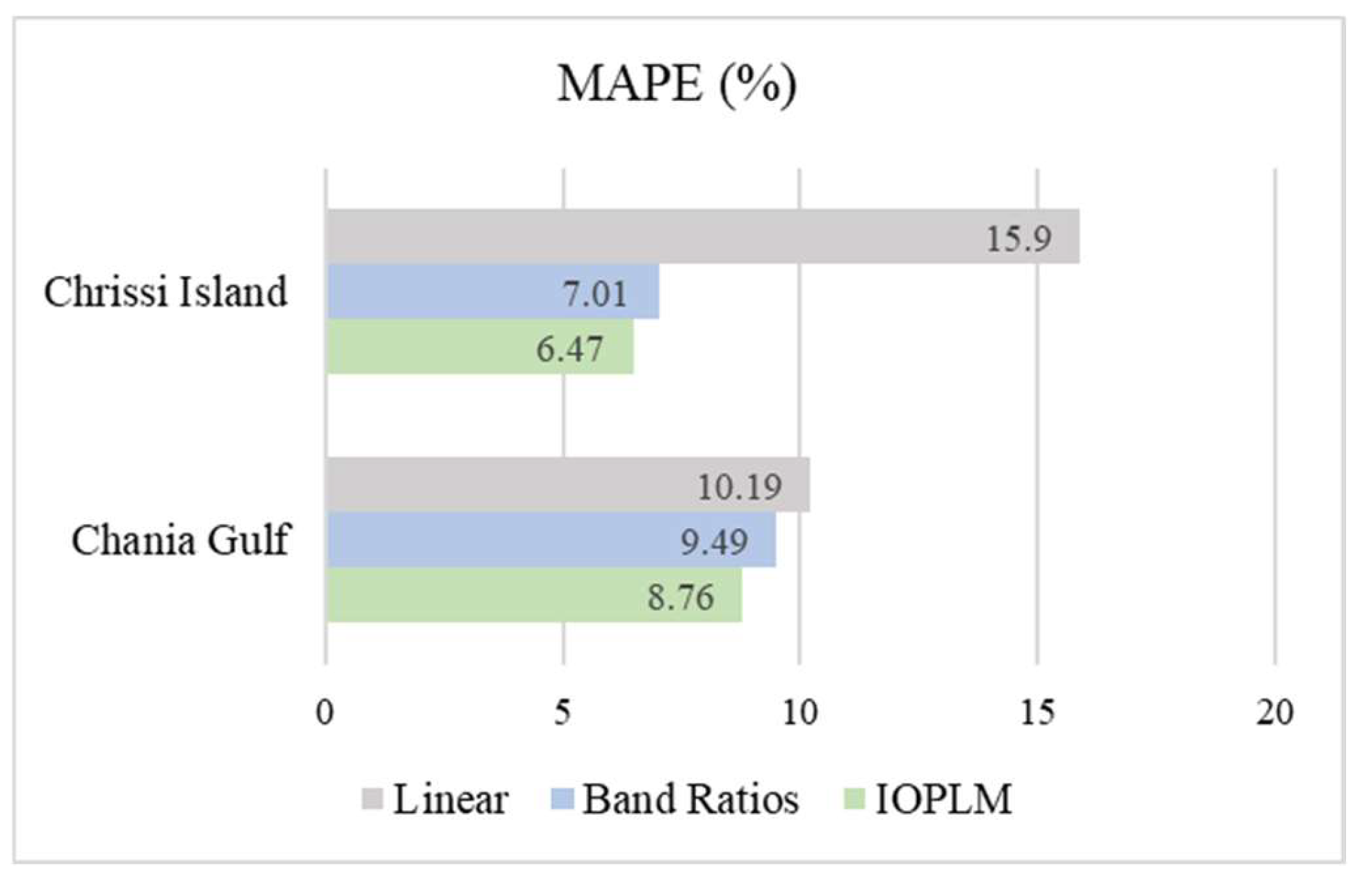
Concluding this subsection, MAPE was determined by utilizing the best results over each year among the three methods for both study sites. The core aim of this investigation was to evaluate the two water bodies’ unique characteristics and the effectiveness of the SDB methods under the premise that using the same passive satellite sensor with identical filtering options would yield imagery with consistent quality attributes. Figure x represents every method’s calculated mean MAPE value for both study areas.
Figure 4.
MAPE Metric Evaluation of SDB Methods Concerning both Study Sites.
The Linear method was presented to overestimate depths even during its optimal performance. This was evident in the western shallow part of the island, where the depth variations between 7 m and 10 m were not adequately displayed. Similar behavior was recorded in the southern rocky seabed, where erroneous reflectances and depth estimation occurred. The other two methods that count for the actual band responses described the bathymetry variations more effectively.
The remote sensing reflectance (Rrs) value showed peak response in the green band (560 nm) regarding very shallow waters, followed by the blue band (490 nm) and the coastal blue (443 nm) band with lower values. In contrast, in shallow and intermediate waters, the transition between the band’s response was smooth, with the blue band (490 nm) maintaining the highest values, closely followed by green (560 nm) and lower coastal blue (443 nm). As the depth increased, the responses of the coastal blue and blue bands converged, while the green band’s response was consistently lower, and over 21 m in deep areas, the response of coastal blue dominates against the others; however, this behavior seemed erroneous.
The above responses indicate the Linear method’s primary exploitation of the green band for its depth estimates, and combinations of coastal blue and blue against the green band were prevalent in ratio-based methods. The level of reflectance observed in deeper regions, approaching 23 m, served as a compelling indicator of the water’s transparency and the SDB’s ability to estimate depths up to this point. It was noted that the remote sensing reflectances among the different products over the study period slightly differ due to the shallow magnitude of these values; however, this slight deviation could make the difference for an accurate SDB estimation.
In areas around Chrissi Island featuring steeper depth gradients, the precision of satellite-derived depth estimates showed a decline, as indicated in the bathymetry plot for both regions in Figure 6 and Figure 7. This reduction in accuracy was particularly noticeable during summer and autumn, especially for depths exceeding 20 m. The impact was most significant in the Linear method and Band Ratio transformation. Factors like shadowing effects and water column optical properties variations contributed to less accurate estimates. However, the IOPLM method, designed to account for inherent optical properties directly, was more successful in mitigating these challenges. The multispectral image’s coastal blue or blue with green band combinations showed a closer relation to depth changes and provided more accurate information. Figure 5 illustrates a set of samples gathered in the island’s northern part (summer 2022) ranging from very shallow waters to deep to investigate the remote sensing response over depth changes. After the C2RCC atmospheric correction and sunglint effect removal, the satellite image was taken.
The variability in the optical milieu of Chania Gulf posed challenges for satellite-derived bathymetry in specific seasons, most notably when influenced by local river runoff. Despite these challenges, the general transparency of the water remained evident. The Linear method displayed remarkable performance in the Chania Gulf compared to Chrissi Island. The Band Ratio transformation likewise showed exceptional and consistent capabilities in feature mapping across all seasons, albeit with minor fluctuations during instances with elevated turbidity. The IOPLM method was similarly proficient in capturing bathymetric variations in the gulf, yielding dependable outcomes. Nonetheless, the method displayed heightened sensitivity to changes in IOPs during reduced water clarity, whether caused by river runoff or wind-induced shallow water mixing.
The maximum depth estimations were slightly lower across all methods in deeper areas, particularly during late summer and autumn. The western part of the gulf, which primarily comprises sandy seabed, was mapped more accurately than the eastern half, dominated by rocky outcrops. This disparity could be due to the difference in bottom albedo, with sandy constituents reflecting lighter than the darker rocks. In addition, the gradual shift from shallow to deep waters in the gulf contributed to better performance, particularly for the Linear method. The maximum reliable depth estimation was slightly lower than Chrissi Island, close to 21 m.
4.3. Assessment of Model Accuracy
Figure 9 demonstrates the most favorable result for this study site, obtained using the IOPLM method during autumn of 2021. An RMSE value of 0.54 m was achieved compared to in-situ measurements, which serve as the reference standard. Additionally, boundaries for CATZOC B adjusted to a depth of 24 m, under IHO’s guidelines, were incorporated into the plot to validate the bathymetric estimates, as illustrated in Figure 8. The total number of individual depth estimates laid into these boundaries was 20 out of 21 (95.24 %), delineating the high accuracy of the SDB outcome even in depths of 24 m.
In assessing bathymetry mapping methods for Chrissi Island, the Linear technique underperformed compared to ratio-based methods as seen in Figure 9. It overestimated depths in the western shallow and southern rocky areas, with RMSE values ranging from 1.18 m to 1.90 m. In contrast, the Band-Ratio and IOPLM methods achieved superior results, with best RMSE values of 0.76 m and 0.54 m, and worst values of 1.68 m and 1.65 m, respectively. The Linear method’s overestimation was likely due to rocky outcrops absorbing more light, affecting depth readings, particularly in the northeastern region (6 to 12 m depth). The Band-Ratio and IOPLM methods proved more robust, with IOPLM being the most suitable for the area, especially when using high-quality Sentinel-2 MSI imagery during winter and spring, processed with the ACOLITE DSF atmospheric correction algorithm.
In Chania Gulf, performance varied significantly among methods, mainly due to late spring turbidity changes from local river runoff. The IOPLM method was particularly sensitive to these variations. The Linear method excelled in summer 2021 with an RMSE of 0.68 m but struggled in autumn 2019, recording an RMSE of 2.07 m, indicating major overestimation. The Band-Ratio technique also performed well, achieving an RMSE of 0.64 m in summer 2018, but its performance declined in summer 2019 (2.12 m RMSE), primarily underestimating depths in the eastern area. IOPLM’s best performance was in spring 2021 (0.86 m RMSE), while its least effective result was in spring 2019 (2.40 m RMSE), showing significant underestimation, particularly in the eastern gulf.
The Linear method’s poor performance was attributed to its reliance on a single spectral band, limiting its adaptability to changing water properties. In contrast, the ratio-based methods, particularly IOPLM, were sensitive to variations, notably in 2019, capturing depth estimations influenced by river inflows. Given the geographic conditions and the quality of Sentinel-2 MSI imagery, the Band-Ratio technique emerged as the most versatile method, especially in late summer or early autumn. While the ACOLITE DSF algorithm was effective, the C2RCC processor also performed well in summer, particularly under severe sunglint, delivering notable results alongside the Linear method.
4.4. Kalman Filter (KF)
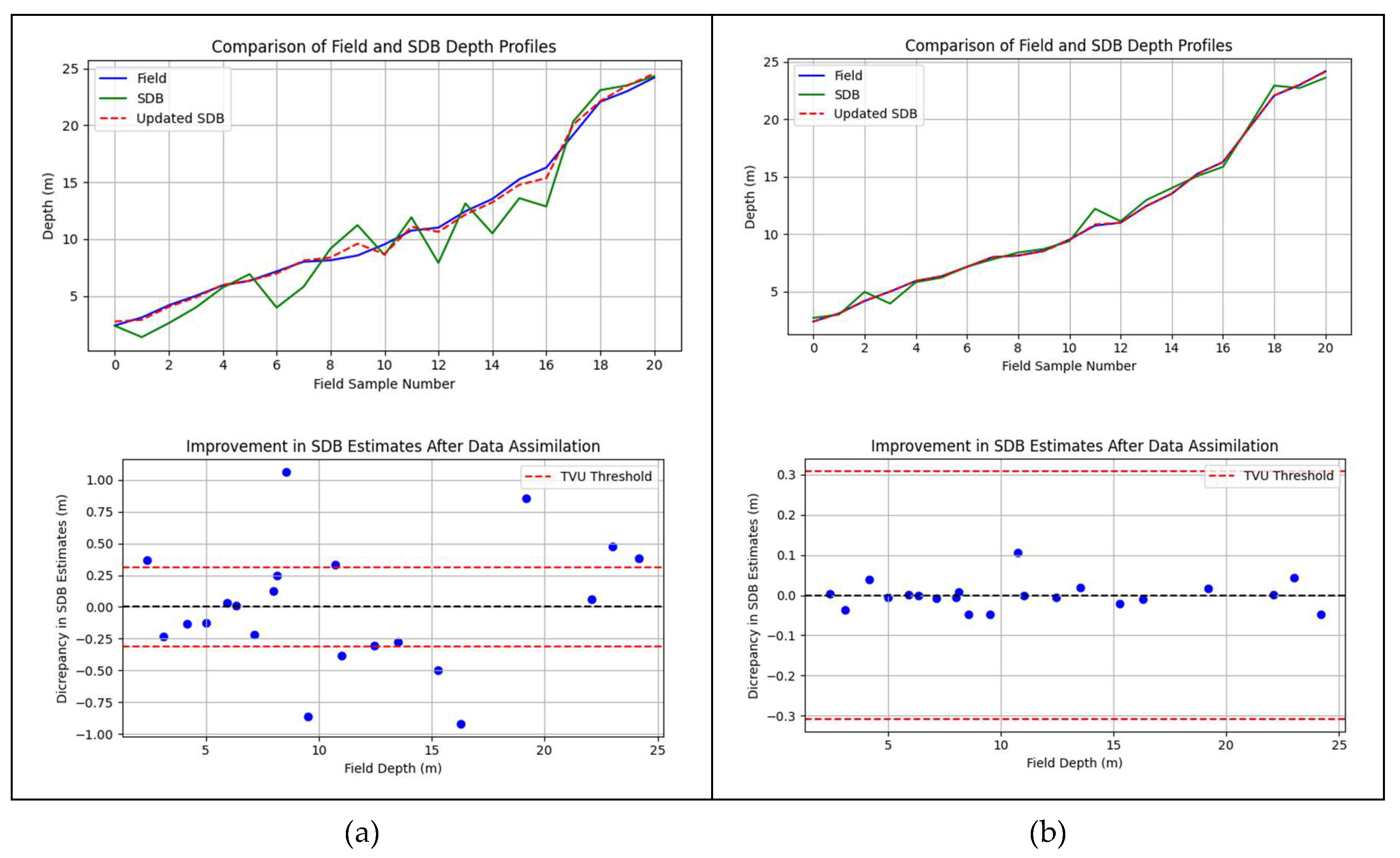
Data assimilation methods, such as Kalman filtering, effectively extract information from noisy observations. When combined with a physics-based model, this approach provides accurate bathymetry estimates and an uncertainty assessment [38]. Applying the Kalman filter significantly reduces estimation errors and results in smoother data outputs. Figure 9 illustrates the results after applying the filter to the Chrissi Island study area using the Linear and IOPLM methods. The filter was applied to the Linear SDB estimates, which show more significant depth discrepancy to the field data, and the IOPLM method, which provides more precise depth estimates. The Kalman filter smooths the best SDB estimates and improves accuracy at greater distances. However, for linear estimates, only 51% of the data samples fall within the TVU range, in contrast with IOPLM data that falls 100% within the TVU.
The performance of the SDB estimation methods shows significant improvement after applying an update, as indicated in Table 2. Initially, the Linear method exhibits high error rates due to using lower-quality sample data, with an RMSE of 1.81, MAE of 1.48, and MedAE of 1.16. After the update, these errors are substantially reduced: RMSE decreases to 0.47, MAE to 0.37, and MedAE to 0.30, reflecting a marked enhancement in accuracy. In contrast, the IOPLM method starts with much lower error rates—an RMSE of 0.54, MAE of 0.40, and MedAE of 0.27—and the update further enhances its performance, reducing RMSE to 0.05, MAE to 0.04, and MedAE to 0.02. It is important to note that the filter was applied to sample data. Further investigation is necessary when working with the entire area generated by SDB and time series data, especially concerning error prediction, modelling, and refining the SDB algorithms. Nevertheless, the method’s ability to dynamically adapt is evident.
5. Conclusions
The research extensively explored the complexities and nuances of Satellite-Derived Bathymetry (SDB) in the Eastern Mediterranean. The study’s multifaceted approach, which considers the region’s unique hydrodynamic characteristics, spatio-temporal variations, and optical properties variations, significantly contributed to the knowledge of the specific field. The study underscored the critical role that spatio-temporal variations play in the accuracy of SDB estimates. The significance of these variations cannot be overstated; they served as a foundation for developing new methodologies and refining existing ones to improve data reliability in hydro-spatial applications.
One of the most significant findings of this research was the strong correlation between water column optical properties and SDB estimates. Explicitly identifying this correlation could enable researchers and practitioners to develop more accurate models for bathymetric estimation. Moreover, the need for concurrent data on optical properties and bathymetry has been substantiated, offering a more holistic approach to underwater mapping and analysis. The in-depth comparative analysis of various SDB methods provided actionable insights into their performance under different conditions over approximately five years. The study identified specific methods that offer higher reliability in correlation with the optical properties of the Eastern Mediterranean. This is critical for decision-makers who must choose the most appropriate method for their specific needs, thereby enhancing the quality and reliability of hydro-spatial data.
By combining different SDB methods into merged products, the study achieved unprecedented accuracy and reliability in bathymetric estimates. This multi-method approach represents a significant advancement in the field, suggesting a new standard for future research and applications. It shows that the robustness and reliability of these merged products offer tangible benefits for applications that require a high degree of precision, such as navigation safety and marine conservation efforts. The study’s findings on the influence of seasonal and weather patterns on SDB estimates provide valuable insights for future research and applications. These findings have practical implications, as they assist researchers and practitioners in planning data collection schedules to avoid times when turbidity or other factors may affect accuracy. Thus, understanding these patterns can lead to more strategic data collection and better outcomes.
While the primary focus of the research was to investigate known variables, unexpected findings also emerged. These anomalies in SDB method performance under unique conditions offer opportunities for further investigation. Unpacking these unexpected findings could pave the way for new research directions, leading to a deeper understanding of SDB methodologies and their limitations. While all three methods offer valuable insights into Chrissi Island’s bathymetry models, their performance varies with seasons and the corresponding optical properties fluctuations. The IOPLM method, given its sophisticated approach, consistently emerges as the most reliable across both regions. Understanding the interplay between these methods, optical properties, and depth profiles is crucial for informed marine and coastal management decision-making. Correlating the variations in optical properties with the method statistics reveals that seasons with higher turbidity or significant suspended matter can hinder the accuracy of satellite-derived bathymetry, especially for the Linear method. Such particles scatter light differently, affecting the satellite’s ability to discern depth based on reflectance alone
6. Future Research
While SDB technology has advanced markedly, challenges around fluid dynamics, ocean colour, and clarity impact modelling. Consequently, over the past two years, a growing trend has investigated the feasibility of deriving bathymetric information in coastal regions solely through satellite-based spatial data. [20,39]. Launched in September 2018, the Ice, Cloud, and Elevation Satellite-2 (ICESat-2) features the Advanced Topographic Laser Altimeter System (ATLAS), a photon-counting lidar operating at a wavelength of 532 nm. Initial data from ICESat-2 have underscored its capability to provide global bathymetric lidar measurements in shallow coastal waters with depths less than 40 m, which can be fused with multispectral imagery and generate SDB estimates. Furthermore, advancements in Machine Learning (ML) algorithms and Artificial Intelligence (AI) could potentially automate processing further and reduce limitations imposed by user-software interaction and data volume [2,9,40].
In summary, satellite-derived bathymetry has made tremendous advances enabled by improved sensors and algorithms. While challenges remain, continued technological improvements indicate its increasing role in coastal mapping applications as a supplemental survey method, offering cost-effective seabed data for regions not yet covered by more uncertain acoustic or LiDAR sensors, given the right environmental conditions. Its cost-efficiency, spatial coverage, and timeliness make it a strong choice for various hydro-spatial tasks. These include scouting remote areas, mapping extremely shallow zones that pose navigational risks, and routinely tracking changes in shallow sea floors [41].
Author Contributions
Conceptualization, F.M. and H.S.; methodology, I.T.; software, I.T.; validation, F.M. and I.T.; formal analysis, I.T.; investigation, F.M. and I.T.; resources, I.T.; data curation, I.T.; writing—original draft preparation, F.M and I.T.; writing—review and editing, F.M.; visualization, F.M and I.T.; supervision, H.S. All authors have read and agreed to the published version of the manuscript.
Funding
This research received no external funding.
Data Availability Statement
the satellite imagery data is openly accessible via the ESA portal. The terrestrial data for training and model validation can be inquired via email to the corresponding author
Acknowledgements
The author would like to thank the ESA for providing free open-access satellite imagery. In addition, the author would like to thank the Greek navy for providing the field data.
Conflicts of Interest
The authors declare no conflicts of interest.
References
- Ashphaq, M.; Srivastava, P.K.; Mitra, D. Review of Near-Shore Satellite Derived Bathymetry: Classification and Account of Five Decades of Coastal Bathymetry Research. J. Ocean Eng. Sci. 2021, 6, 340–359. [CrossRef]
- Louvart, P.; Cook, H.; Smithers, C.; Laporte, J. A New Approach to Satellite-Derived Bathymetry: An Exercise in Seabed 2030 Coastal Surveys. Remote Sens. 2022, 14. [CrossRef]
- Stumpf, R.P.; Holderied, K.; Spring, S.; Sinclair, M. Determination of Water Depth with High-Resolution Satellite Imagery over Variable Bottom Types. 2003, 48, 547–556.
- Lyzenga, D. Passive Remote-Sensing Techniques for Mapping Water Depth and Bottom Features. Appl. Opt. 1978. [CrossRef]
- Jupp, D. International Journal of Remote Reconstruction of Sand Wave Bathymetry Using Both Satellite Imagery and Multi-Beam Bathymetric Data : A Case Study of the Taiwan Banks. In Proceedings of the Proceedings of the Symposium on Remote Sensing of the Coastal Zone; Gold Coast, Queensland, Australia, 1988.
- Lee, Z.; Carder, K.L.; Arnone, R.A. Deriving Inherent Optical Properties from Water Color: A Multiband Quasi-Analytical Algorithm for Optically Deep Waters. Appl. Opt. 2002, 41, 5755. [CrossRef]
- Zhang, X.; Ma, Y.; Zhang, J. Shallow Water Bathymetry Based on Inherent Optical Properties Using High Spatial Resolution Multispectral Imagery. Remote Sens. 2020, 12. [CrossRef]
- Streftaris, N.; Zenetos, A.; Papathanassiou, E. Globalisation in Marine Ecosystems: The Story of Non-Indigenous Marine Species across European Seas. Oceanogr. Mar. Biol. 2005, 43, 419–453. [CrossRef]
- Mandlburger, G. A Review of Active and Passive Optical Methods in Hydrography. Int. Hydrogr. Rev. 2022, 28, 8–52. [CrossRef]
- Chaikalis, S.; Parinos, C.; Möbius, J.; Gogou, A.; Velaoras, D.; Hainbucher, D.; Sofianos, S.; Tanhua, T.; Cardin, V.; Proestakis, E.; et al. Optical Properties and Biochemical Indices of Marine Particles in the Open Mediterranean Sea: The R/V Maria S. Merian Cruise, March 2018. Front. Earth Sci. 2021, 9, 1–20. [CrossRef]
- Drakopoulou, P.; Kapsimalis, V.; Parcharidis, I.; Pavlopoulos, K. Retrieval of Nearshore Bathymetry in the Gulf of Chania, NW Crete, Greece, from WorldWiew-2 Multispectral Imagery. 2018, 54. [CrossRef]
- .
- 2022; 13. ESA S2 MSI ESL Team COPERNICUS SPACE COMPONENT SENTINEL OPTICAL IMAGING MISSION PERFORMANCE CLUSTER SERVICE Sentinel-2 Annual Performance Report-Year 2022; 2023;
- Lyzenga, D. Shallow-Water Bathymetry Using Combined Lidar and Passive Multispectral Scanner Data. Int. J. Remote Sens. 1985, 6, 115–125. [CrossRef]
- Philpot, W.D. Bathymetric Mapping with Passive Multispectral Imagery. Appl. Opt. 1989, 28, 1569. [CrossRef]
- .
- Ribeiro, M.I. Kalman and Extended Kalman Filters : Concept , Derivation and Properties. In Institute for Systems and Robotics Lisboa Portugal; 2004; p. 42.
- Mobley, C.D.; Stramski, D.; Paul Bissett, W.; Boss, E. Optical Modeling of Ocean Waters: Is the Case 1 - Case 2 Classification Still Useful? Oceanography 2004, 17, 60–67. [CrossRef]
- Mobley, C.D. The Oceanic Optics Book. Int. Ocean Colour Coord. Gr. Dartmouth, NS, Canada 2022, 924. [CrossRef]
- Mavraeidopoulos, A.K. Satellite Derived Bathymetry with No Use of Field Data. Int. Sci. Conf. Des. Manag. Harb. Coast. Offshore Work. 2023, 1–8.
- Mavraeidopoulos, A.K.; Oikonomou, E.; Palikaris, A.; Poulos, S. A Hybrid Bio-Optical Transformation for Satellite Bathymetry Modeling Using Sentinel-2 Imagery. Remote Sens. 2019, 11, 1–16. [CrossRef]
- Chavez, P.S. An Improved Dark-Object Subtraction Technique for Atmospheric Scattering Correction of Multispectral Data. Remote Sens. Environ. 1988, 24, 459–479. [CrossRef]
- Goodman, J.A.; Lee, Z.P.; Ustin, S.L. Influence of Atmospheric and Sea-Surface Corrections on Retrieval of Bottom Depth and Reflectance Using a Semi-Analytical Model: A Case Study in Kaneohe Bay, Hawaii. Appl. Opt. 2008, 47. [CrossRef]
- Traganos, D.; Poursanidis, D.; Aggarwal, B.; Chrysoulakis, N.; Reinartz, P. Estimating Satellite-Derived Bathymetry (SDB) with the Google Earth Engine and Sentinel-2. Remote Sens. 2018, 10, 1–18. [CrossRef]
- Hedley, J.D.; Harborne, A.R.; Mumby, P.J. Simple and Robust Removal of Sun Glint for Mapping Shallow-Water Benthos. Int. J. Remote Sens. 2005, 26, 2107–2112. [CrossRef]
- 2 August 2021; 26. RBINS ACOLITE User Manual (QV - August 2,2021); Royal Belgian Institute of Natural Sciences (RBINS), Belgium, 2021;
- Vanhellemont, Q. Adaptation of the Dark Spectrum Fitting Atmospheric Correction for Aquatic Applications of the Landsat and Sentinel-2 Archives. Remote Sens. Environ. 2019, 225, 175–192. [CrossRef]
- Doerffer, R.; Schiller, H. The MERIS Case 2 Water Algorithm. Int. J. Remote Sens. 2007, 28, 517–535. [CrossRef]
- Brockman, C.; Doerffer, R.; Peters, M.; Stelzer, K.; Embacher, S.; Ruescas, A. Evolution of the C2RCC Neural Network for Sentinel 2 and 3 for the Retrieval of Ocean Colour Products in Normal and Extreme Optically Complex Waters. 2004, 1–14.
- Hollingsworth, A.; Engelen, R.J.; Textor, C.; Benedetti, A.; Boucher, O.; Chevallier, F.; Dethof, A.; Elbern, H.; Eskes, H.; Flemming, J.; et al. Toward a Monitoring and Forecasting System for Atmospheric Composition: The GEMS Project. Bull. Am. Meteorol. Soc. 2008, 89, 1147–1164. [CrossRef]
- Caballero, I.; Stumpf, R.P. Atmospheric Correction for Satellite-Derived Bathymetry in the Caribbean Waters: From a Single Image to Multi-Temporal Approaches Using Sentinel-2A/B. Opt. Express 2020, 28, 11742. [CrossRef]
- Nechad, B.; Ruddick, K.G.; Neukermans, G. Calibration and Validation of a Generic Multisensor Algorithm for Mapping of Turbidity in Coastal Waters. Remote Sens. Ocean. Sea Ice, Large Water Reg. 2009 2009, 7473, 74730H. [CrossRef]
- Nechad, B.; Ruddick, K.G.; Park, Y. Calibration and Validation of a Generic Multisensor Algorithm for Mapping of Total Suspended Matter in Turbid Waters. Remote Sens. Environ. 2010, 114, 854–866. [CrossRef]
- Chai, T.; Draxler, R.R. Root Mean Square Error (RMSE) or Mean Absolute Error (MAE)? -Arguments against Avoiding RMSE in the Literature. Geosci. Model Dev. 2014, 7, 1247–1250. [CrossRef]
- Willmott, C.J.; Matsuura, K. Advantages of the Mean Absolute Error (MAE) over the Root Mean Square Error (RMSE) in Assessing Average Model Performance. Clim. Res. 2005, 30, 79–82. [CrossRef]
- Makridakis, S. Accuracy Measures: Theoretical and Practical Concerns. Int. J. Forecast. 1993, 9, 527–529. [CrossRef]
- I: S-44 6th Edition, 2020; 37. IHO S-44 6th Edition: IHO Standards For Hydrographic Surveys; Monaco, 2020;
- Ghorbanidehno, H.; Lee, J.; Farthing, M.; Hesser, T.; Kitanidis, P.K.; Darve, E.F. Novel Data Assimilation Algorithm for Nearshore Bathymetry. J. Atmos. Ocean. Technol. 2019, 36, 699–715. [CrossRef]
- Thomas, N.; Pertiwi, A.P.; Traganos, D.; Lagomasino, D.; Poursanidis, D.; Moreno, S.; Fatoyinbo, L. Space-Borne Cloud-Native Satellite-Derived Bathymetry (SDB) Models Using ICESat-2 And Sentinel-2. Geophys. Res. Lett. 2021, 48, 1–11. [CrossRef]
- Mohamed, H.; Nadaoka, K.; Nakamura, T. Towards Benthic Habitat 3D Mapping Using Machine Learning Algorithms and Structures from Motion Photogrammetry. 2020.
- Herrmann, J.; Magruder, L.A.; Markel, J.; Parrish, C.E. Assessing the Ability to Quantify Bathymetric Change over Time Using Solely Satellite-Based Measurements. Remote Sens. 2022, 14, 1–15. [CrossRef]
Figure 1.
The study area is situated in the Cretan Sea and divided into AOI (a) the Chania Gulf, and (b) Chrissi Island.
Figure 1.
The study area is situated in the Cretan Sea and divided into AOI (a) the Chania Gulf, and (b) Chrissi Island.
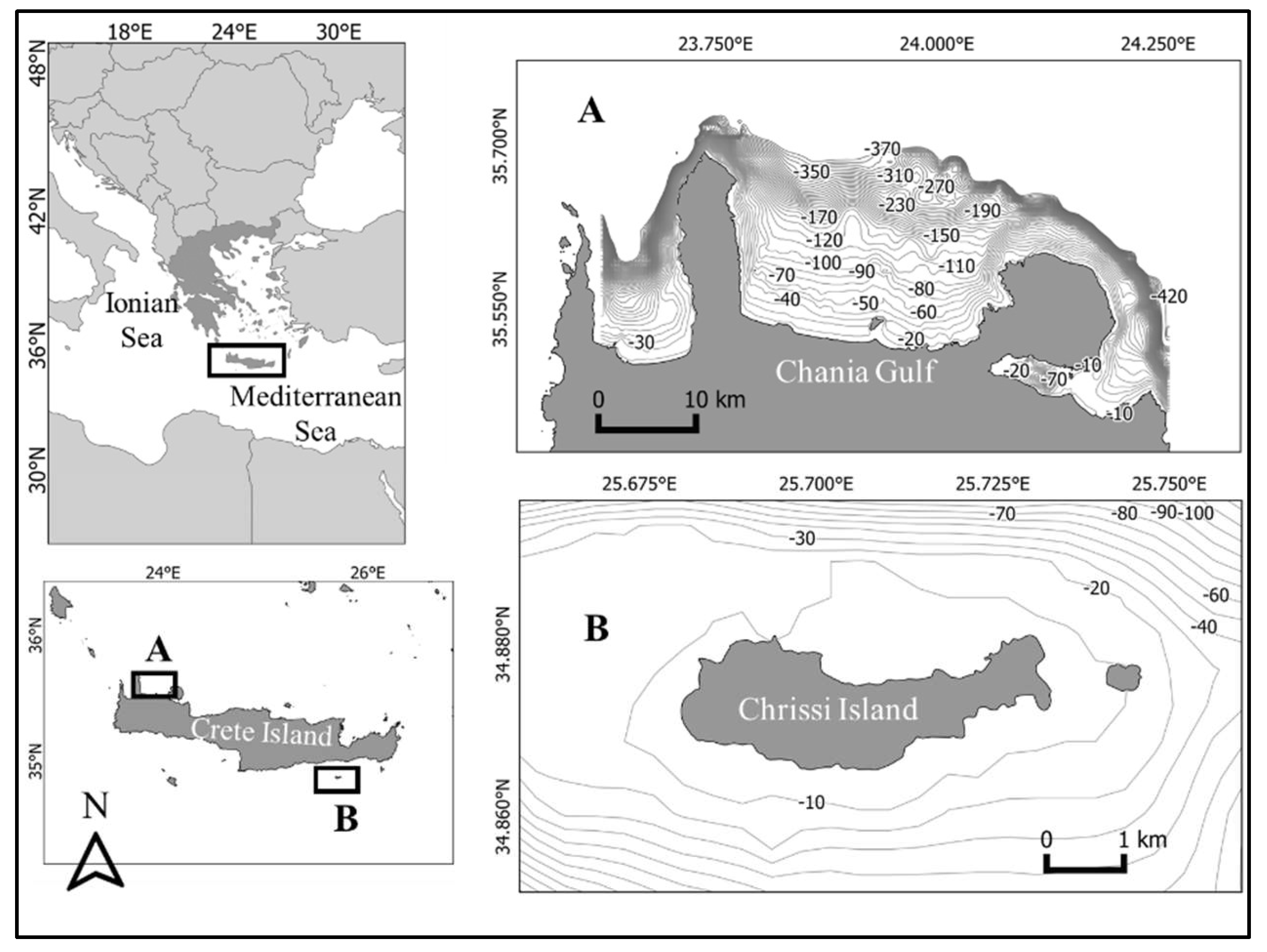
Figure 2.
Figure 2. Illustration of SDB workflow processing.
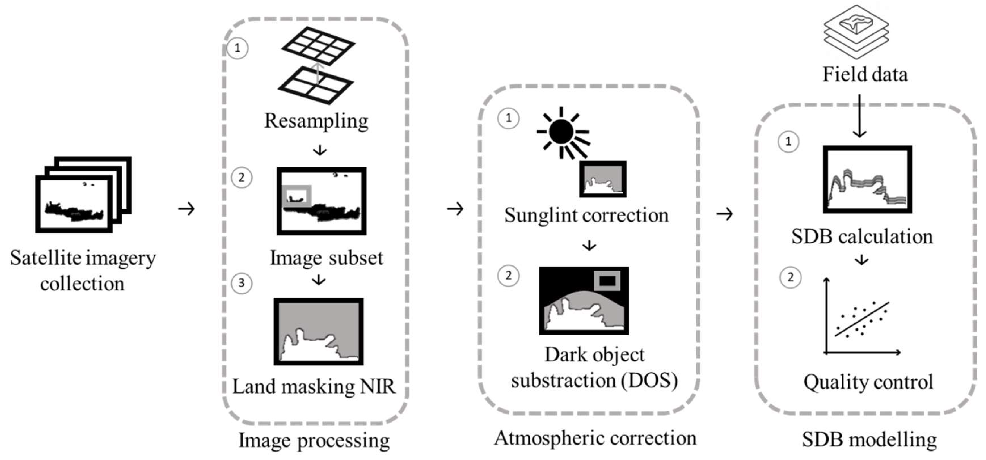
Figure 3.
Typical AOP and IOP’s variations in a seasonal basis in 2020 for (a) Chania Gulf and (b) Chrissi Island.
Figure 3.
Typical AOP and IOP’s variations in a seasonal basis in 2020 for (a) Chania Gulf and (b) Chrissi Island.
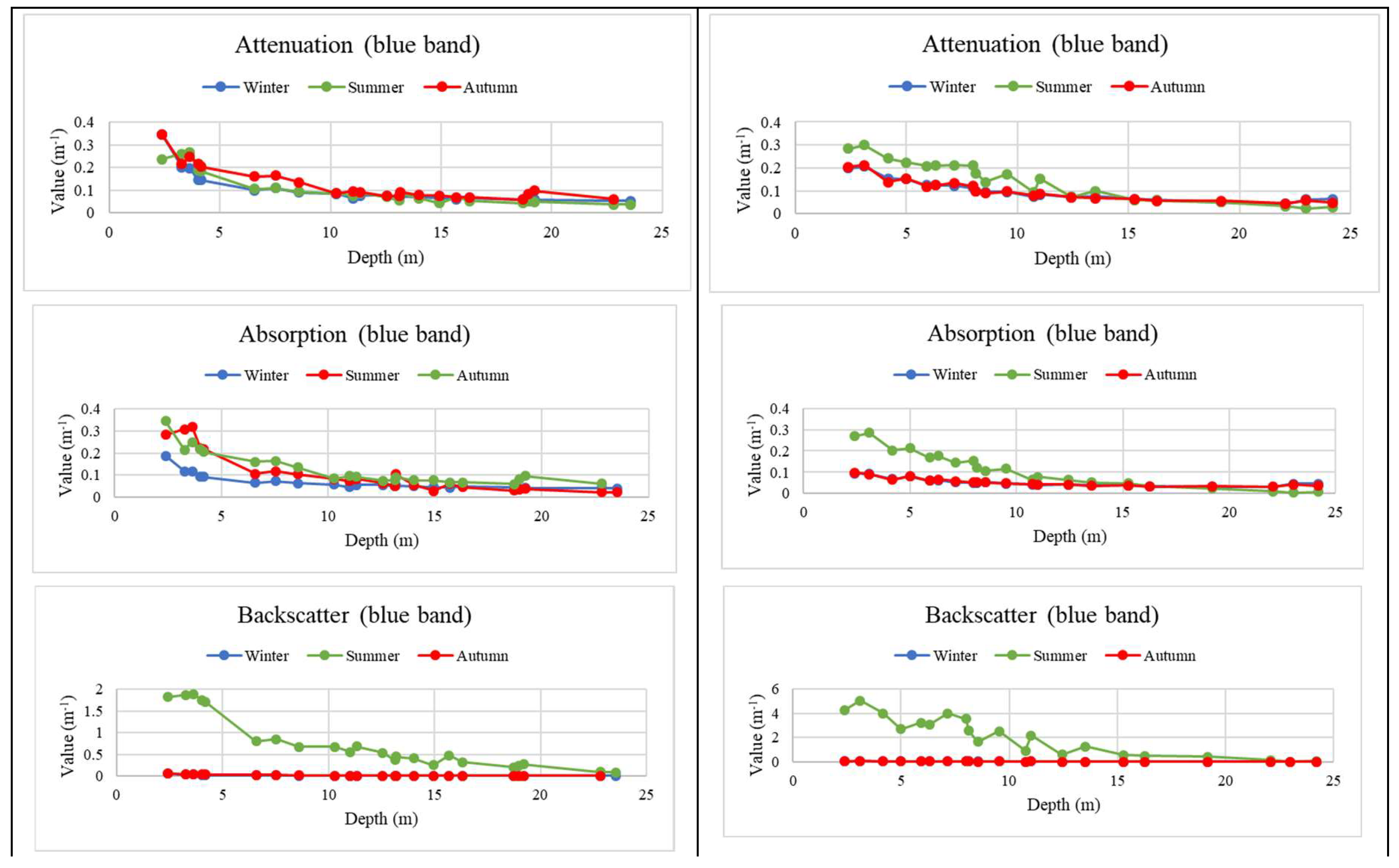
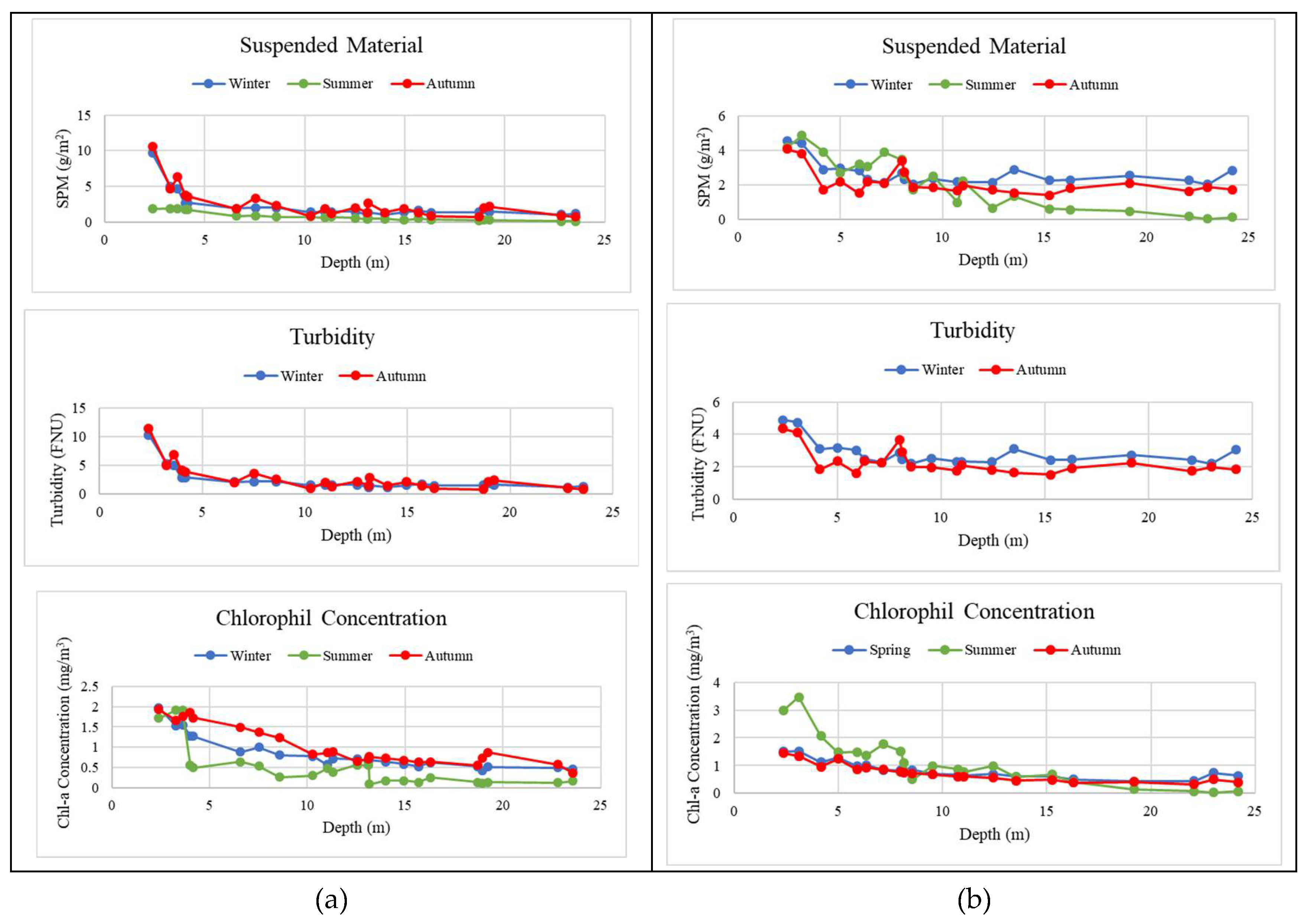
Figure 4.
Error metrics of SDB estimates across all seasons for (a) Chania Gulf and (b) Chrissi Island.
Figure 4.
Error metrics of SDB estimates across all seasons for (a) Chania Gulf and (b) Chrissi Island.
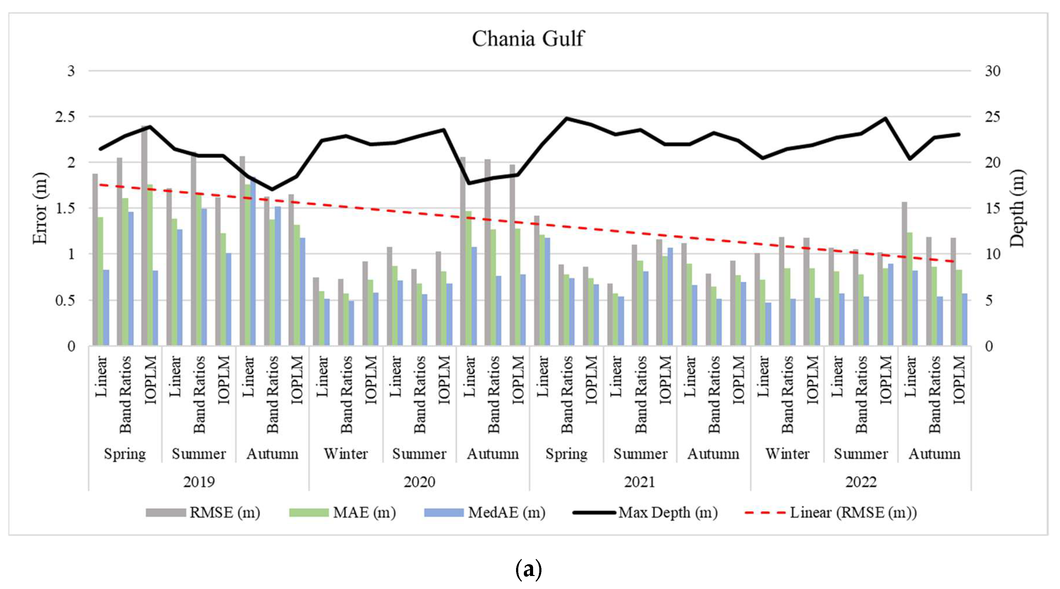
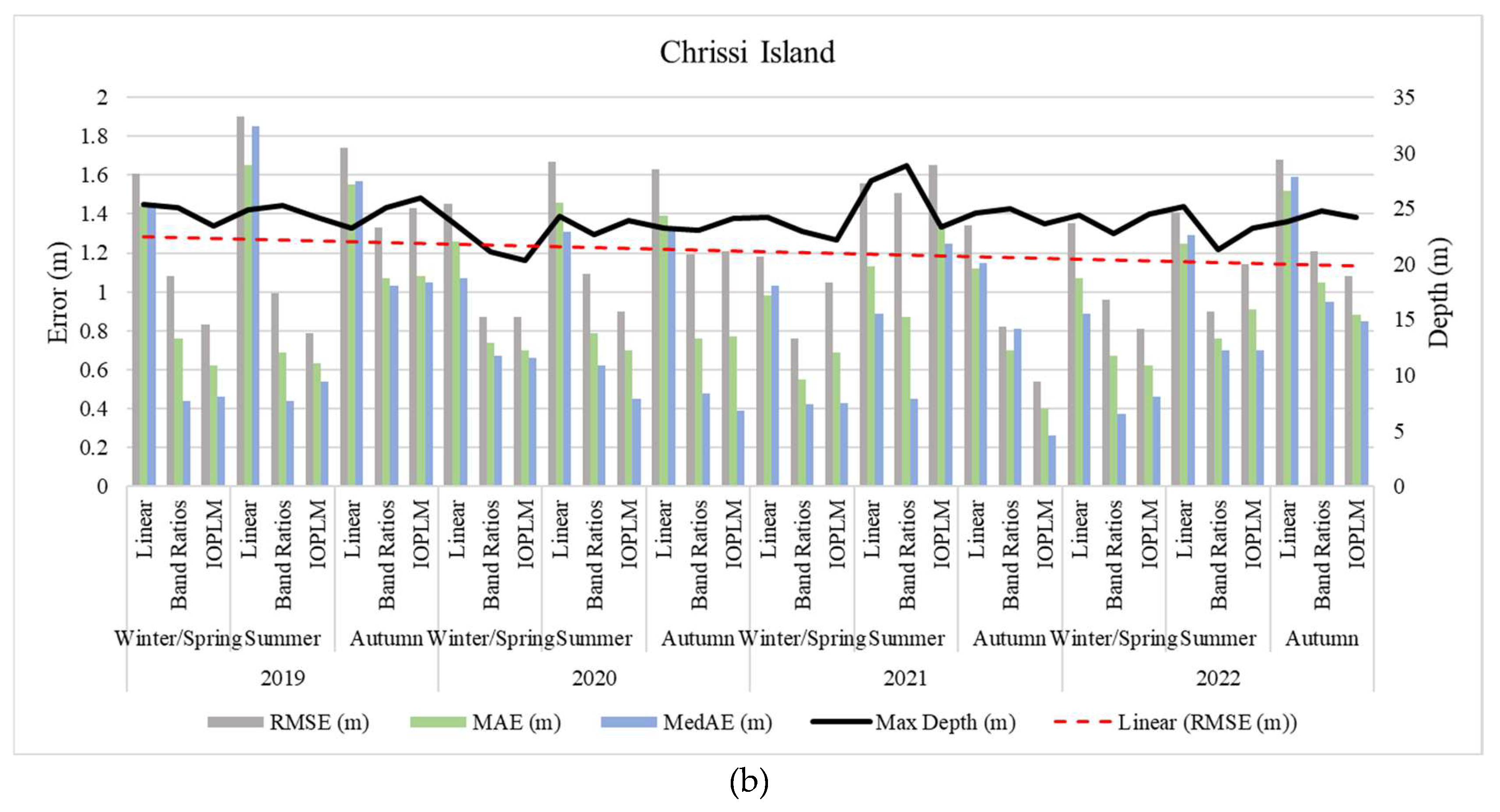
Figure 5.
Spectrum Analysis Concerning Remote Sensing Reflectance (Rrs).
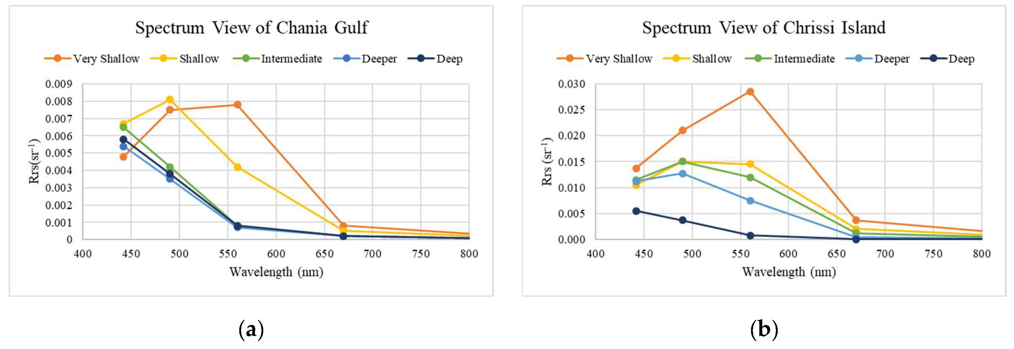
Figure 6.
Typical SDB model in Chania Gulf: (a) Autumn, (b) Winter/Spring, and (c) Summer.
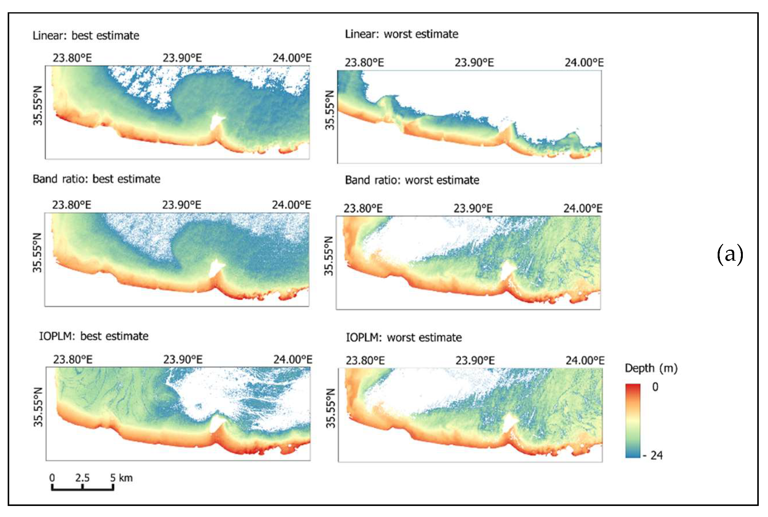
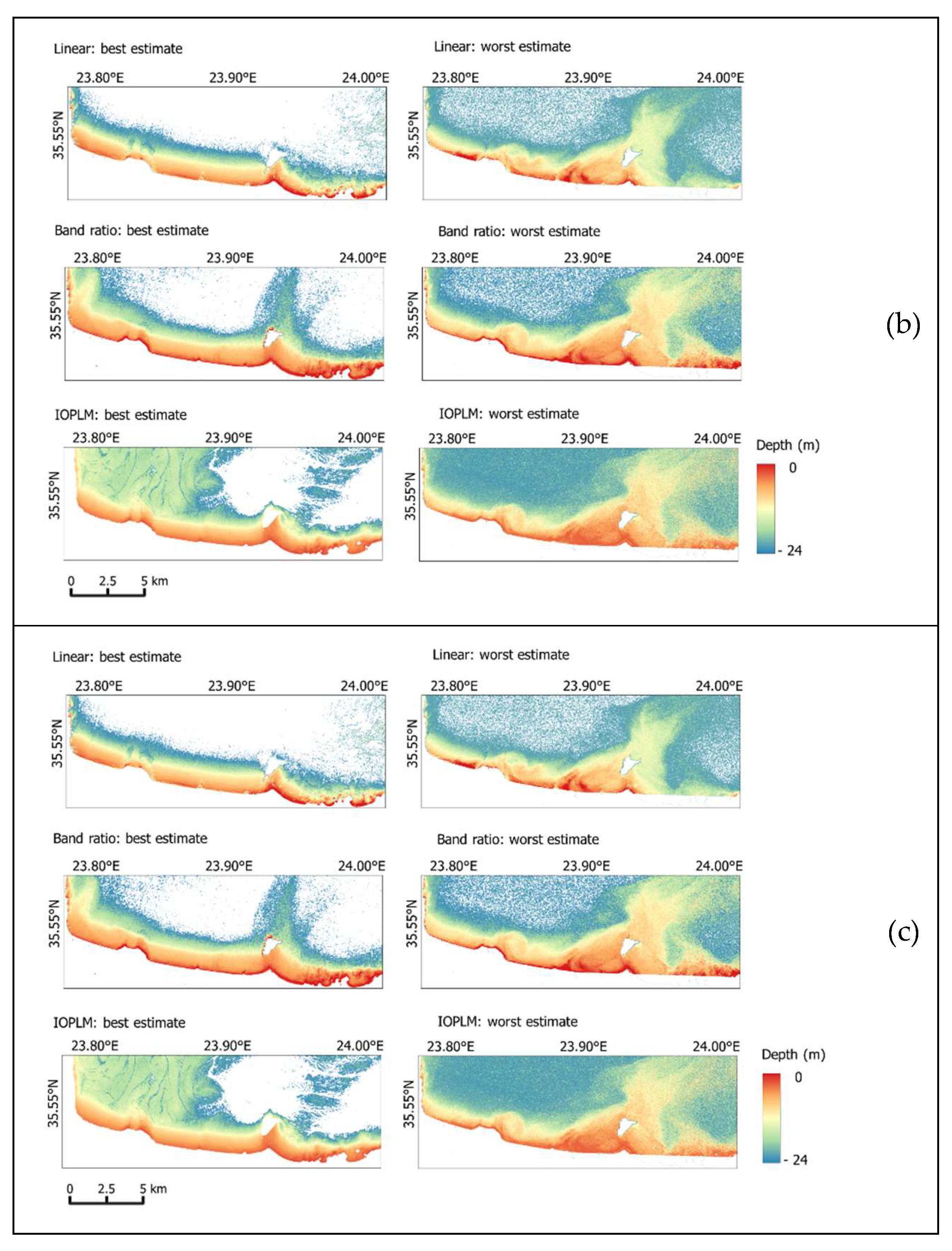
Figure 7.
Typical SDB model in Chrissi Island: (a) Autumn, (b) Winter/Spring, and (c) Summer.
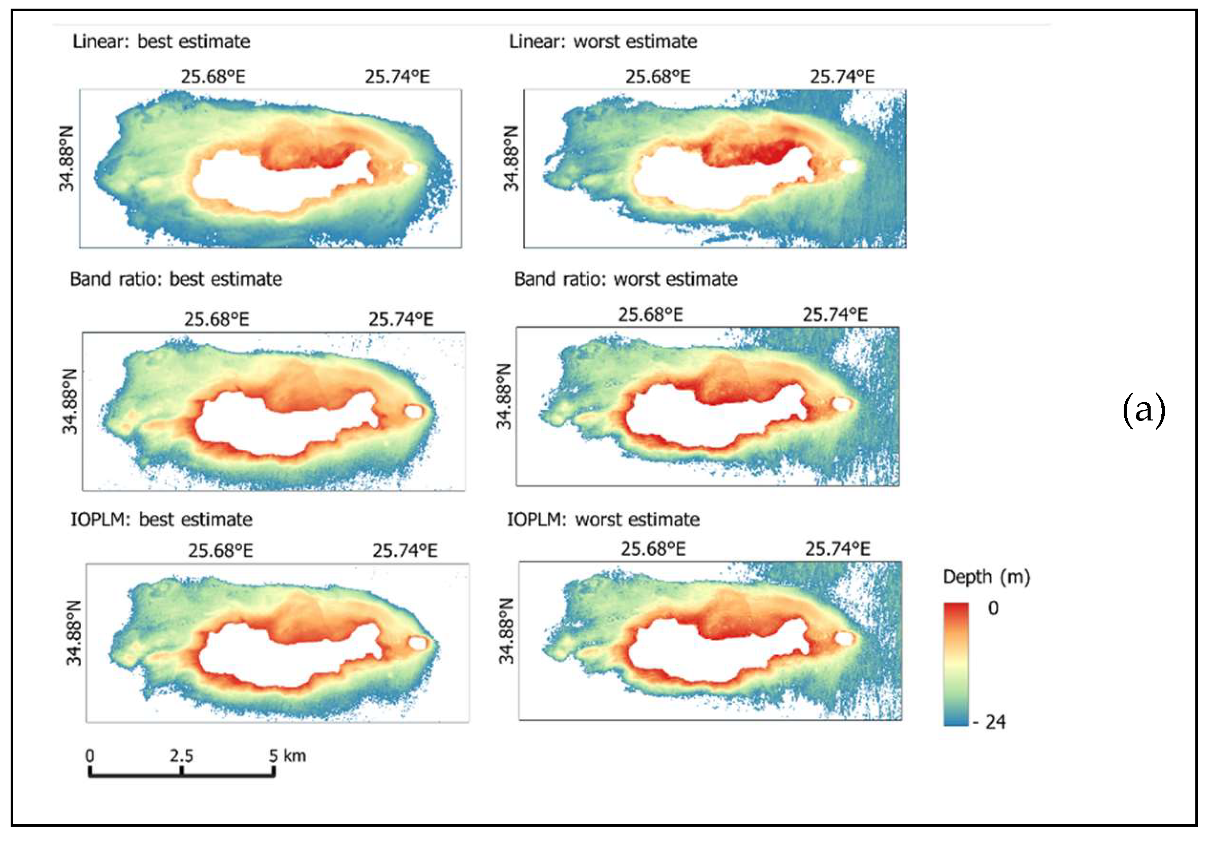
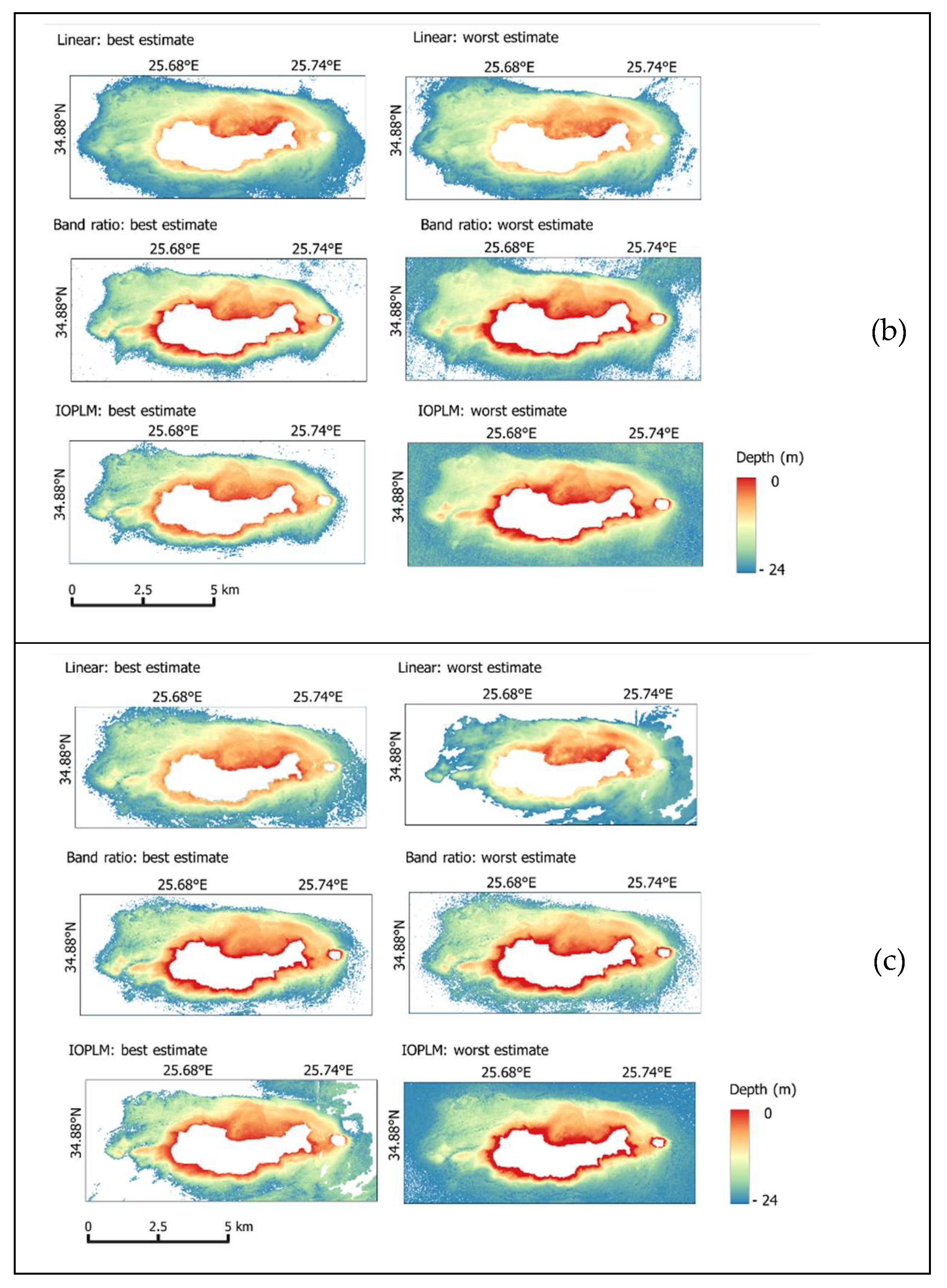
Figure 8.
Error classification of SDB model based on CATZOC: (a) Chania Gulf and (b) Chrissi Island.
Figure 8.
Error classification of SDB model based on CATZOC: (a) Chania Gulf and (b) Chrissi Island.
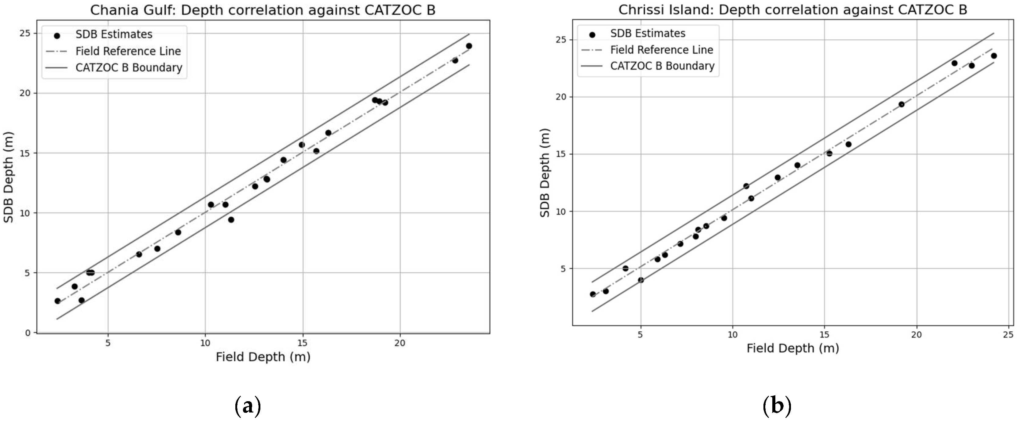
Figure 9.
Multi-Bathymetric Plot for Chrissi Island: The first row (1) shows the Linear method’s best performance on the left and least on the right. The second row (2) presents the Band-Ratio method’s best on the left and least on the right. The third row (3) displays the IOPLM method’s best on the left and least on the right.
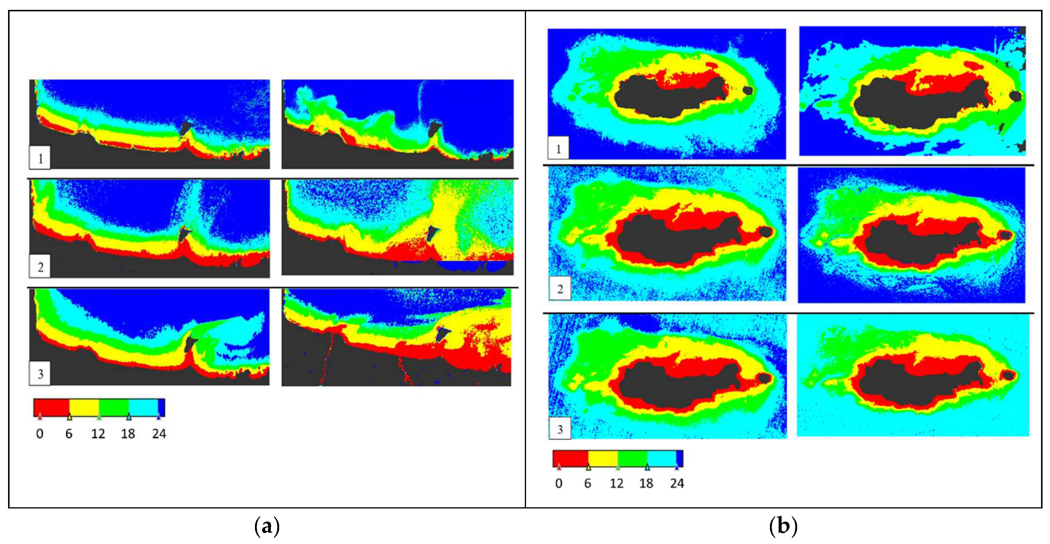
Figure 9.
SDB Linear Method’s Estimations Before and After KF Employment for Chrissi Island Case: (a) Linear SDB estimates and (b) IOPLM SDB estimates.
Figure 9.
SDB Linear Method’s Estimations Before and After KF Employment for Chrissi Island Case: (a) Linear SDB estimates and (b) IOPLM SDB estimates.

| Year | Season | Sensing Date (UTC time) | Cloud Coverage (%) | Sun Zenith Angle (degree) | Sun Azimuth Angle (degree) |
|---|---|---|---|---|---|
| Spring | 19-Mar-2019 / 09:10:46 | 0.2309 | 39.50 | 149.45 | |
| 2019 | Summer | 21-Aug-2019 / 09:10:50 | 0.1704 | 27.70 | 140.30 |
| Autumn | 25-Oct-2019 / 09:10:48 | 0 | 48.36 | 163.00 | |
| Winter | 23-Jan-2020 / 09:10:41 | 0.8564 | 57.44 | 157.70 | |
| 2020 | Summer | 30-Aug-2020 / 09:10:51 | 0 | 30.28 | 145.03 |
| Autumn | 13-Nov-2020 / 09:10:51 | 0.9878 | 54.27 | 164.79 | |
| Spring | 13-Mar-2021 / 09:10:47 | 0.1587 | 41.63 | 150.29 | |
| 2021 | Summer | 30-Aug-2021 / 09:10:49 | 0 | 30.21 | 144.91 |
| Autumn | 24-Oct-2021 / 09:10:49 | 0 | 48.20 | 162.93 | |
| Winter | 11-Feb-2022 / 09:10:42 | 0.3548 | 52.44 | 154.67 | |
| 2022 | Summer | 20-Aug-2022 / 09:10:19 | 0 | 27.53 | 139.93 |
| Autumn | 04-Oct-2022 / 09:10:54 | 1.3555 | 41.31 | 158.50 |
Table 2.
Metrics Response of Linear Method Before and After KF Improvement.
| SDB Method | Metric | Value (m) |
|---|---|---|
| Linear | RMSE | 1.81 |
| RMSE updated | 0.47 | |
| MAE | 1.48 | |
| MAE updated | 0.37 | |
| MedAE | 1.16 | |
| MeadAE updated | 0.30 | |
| IOPLM | RMSE | 0.54 |
| RMSE updated | 0.05 | |
| MAE | 0.40 | |
| MAE updated | 0.04 | |
| MedAE | 0.27 | |
| MeadAE updated | 0.02 |
Disclaimer/Publisher’s Note: The statements, opinions and data contained in all publications are solely those of the individual author(s) and contributor(s) and not of MDPI and/or the editor(s). MDPI and/or the editor(s) disclaim responsibility for any injury to people or property resulting from any ideas, methods, instructions or products referred to in the content. |
© 2024 by the authors. Licensee MDPI, Basel, Switzerland. This article is an open access article distributed under the terms and conditions of the Creative Commons Attribution (CC BY) license (http://creativecommons.org/licenses/by/4.0/).
Copyright: This open access article is published under a Creative Commons CC BY 4.0 license, which permit the free download, distribution, and reuse, provided that the author and preprint are cited in any reuse.


