
Submitted:
06 February 2025
Posted:
07 February 2025
You are already at the latest version
Abstract
This study enhances the accuracy of optical satellite-derived bathymetric datasets in a shallow, mixed benthic, low wave energy coastal environment by identifying the optimal combination of input satellite imagery, spectral bands, and empirical derivation techniques. A total of 109 unique derivations were performed based on an exhaustive combination of these variables. These deri-vations were calibrated and validated using 1,064,536 ground truth observations. Results revealed that the multiband linear technique consistently outperformed the band ratio technique, achieving the best results with input bands from PlanetScope SuperDove imagery. The top-performing derivation attained an R² value of 0.94 and an RMSE of 0.41m when compared with ground truth data, surpassing published RMSE values in similar environments. Further validation beyond the calibration site confirmed its effectiveness within depths of 0.5m to 5m, demonstrating an RMSE of 0.51m, albeit with a gradual reduction in accuracy with increasing depth. This research not only identifies the optimal combination of variables but also provides valuable insights into how the number of input bands, their spatial resolution, and their specific spectral properties (central wavelength and bandwidth) influence the quality of satellite-derived bathymetry datasets. Challenges remain in accounting for mixed benthic types and their variable albedos.
Keywords:
Satellite-derived bathymetry (SDB)
; empirical techniques
; coastal sedimentary environments
; multiband linear technique
; band ratio technique
; Sentinel-2
; PlanetScope SuperDove
; Pleiades Neo
; Benthos
Introduction
Coastal sedimentary nearshore environments inherently exhibit a dynamic nature, displaying variations in both time and space. These environments are comprised of both sub- and supra-aqueous zones, and their morphology is shaped by the existing geology, topography, sediment supply and sea level, and forced by a range of oceanographic and geologic processes [1]. These processes occur on both short and long-term time-scales and drive geomorphic evolution, and they include sea level rise; tides and currents; storm magnitude, frequency, direction, and duration; wind, climatic cycles (e.g. Southern Annular Mode); sand type and supply; and tectonic uplift and subsidence of the coastal zone [2].
Forecasting the evolution of nearshore sedimentary environments as they respond to variations in oceanographic and geologic processes is crucial for ensuring the resilience of coastal areas in the context of climate change. Predictive models like Delft3D and X-beach have been utilised to aid understanding of shoreline change. However, these models are limited by the costly input of up-to-date medium-resolution (1-10m) bathymetric grids and the validation of model outputs through repeat bathymetric surveys [1]. Conventionally, echo sounders and airborne Light Detection and Ranging (LiDAR) bathymetric systems have been utilised to capture these datasets. These are high-precision technologies that are essential for obtaining precise bathymetric information (i.e. within a few centimetres) [3,4], capable of meeting International Hydrographic Organization Standards for Hydrographic Survey [5]. However, these methods have inherent limitations in terms of cost and time constraints [6] and the dynamic nature of the nearshore potentially renders the outputs dataset outdated shortly after the survey has concluded. These cost and time restraints often result in spatially sparse bathymetric observations being interpolated over large distances, with vertical uncertainty being introduced [7]. In contrast, satellite-derived bathymetry (SDB) is cost-effective, non-intrusive, able to survey remote locations, capable of extensive coverage, spatially and temporally continuous, and repeatable at user-defined intervals [8]. Hence, it is a more efficient mechanism for obtaining bathymetric information, albeit with large error margins (root mean square error (RMSE) ~1m) [1,6,9,10,11]. Consequently, SDB may not be suitable for all applications, such as maritime construction or port surveys; however, it is well-suited for coastal monitoring and modelling purposes, where its utility is maximised.
SDB is inferred from both passive and active space-borne sensors, although, more commonly from passive imaging sensors [12]. Passive methods (the focus of this research) relate water leaving radiance to depth based on the Beer-Lambart Law (Eq. 1) which proposes an exponential relationship between the attenuation of light in water and water depth [13]. This law suggests that the remaining water leaving radiance (Id) in a medium (pure water) is a function of incident light intensity (I0) and reduces with increased passage (p). It is also dependent on the specific attenuation coefficient (k) which varies with wavelength. This is expressed by:
Along with SDB being limited by depth, SDB is also limited by other factors that prohibit electromagnetic energy from interacting with the seafloor and being reflected to space-based sensors, including excess turbidity, high sea-states, sea-surface reflectance, and atmospheric scattering [14]. Complex mixed bottom types with spatially variant albedo further contribute to increased uncertainties.
Within optical SDB literature, there are two major approaches commonly cited; empirical and analytical (physics-based) approaches [12,15]. Analytical approaches are based on the radiative transfer of light within a water body and require the input of multiple in situ measurements, including water quality parameters and seafloor albedo [15]. Hence, the approach is limited by the requirement of simultaneous in situ measurements distributed throughout the surveyed area at the time of image capture to account for the fluctuating and spatially variant nature of the nearshore environment [8,15].
Empirical approaches, rather than solving depth based on the physics of light attenuation through a defined medium, typically employ linear and non-linear regressions to estimate depth based solely on corresponding depth observations and the reflectance of single or multiple bands [12]. Traditional empirical approaches in contrast to analytical approaches are simpler to implement and although not as accurate as analytical approaches in heterogeneous environmental conditions, do produce quality results in homogenous environments and at depths less than 20m [15].
An evaluation of SDB dataset quality in an optically shallow, mixed bottom, low wave energy coastal environment derived from diverse space-borne multi-spectral sensors, each possessing unique spectral properties and spatial resolutions, and estimated using different empirical techniques, would greatly assist coastal practitioners both globally and locally, enabling the capture of optimised, cost-effective, spatially, and temporally extensive bathymetric grids. This would increase the capacity to monitor and model coastal sedimentary responses to sea level rise in similar environments and enable coastal practitioners to best manage beach amenity, coastal infrastructure, and coastal ecology on optically shallow, mixed bottom, low wave energy coasts. However, such studies are currently limited in number and scope, warranting further investigation.
Review papers of existing literature do provide meta-analysis of the mean correlation coefficient and RMSE values of many major derivation techniques in a range of coastal environments [3,12]. However, these reviews are constrained by the limited publication of spectral information used in the SDB derivations and the extensive timescale of the sourced literature, leading to a disparity in imaging quality (spatially, spectrally, and radiometrically). More recent work by Evagorou et al. [6] made significant headway in determining an optimised SDB derivation method for a similar environment by empirically testing the best combination of input satellite imagery, input spectral bands, and derivation techniques. However, Evagorou et al. [6] utilised conventional PlanetScope 4-band imagery instead of exploring the potentially superior PlanetScope SuperDove constellation, which offers enhanced spectral resolution in the visible spectrum [16]. This highlights the need for further investigation to fully leverage these advancements.
Furthermore, the relationship between the number of input bands, their spatial resolution, and their specific spectral properties (central wavelength and bandwidth) with output SDB dataset quality remains unknown. Evagorou et al. [6] identified that the impact of spatial resolution of satellite imagery on SDB quality should be a subject of future work. Similarly, the influence of improved spectral sampling of the visible spectrum on dataset quality remains uncertain. While most studies traditionally use green and blue wavelengths for SDB derivations due to their lower absorption by the water column than other visible wavelengths [17,18,19], recent observations suggest that providing more input spectral data to machine learning algorithms enhances accuracy, prompting a shift towards the use of hyper-spectral data for SDB derivations [20,21]. Questions remain as to whether this applies to SDB derivations performed with traditional derivation techniques.
This research aims to enhance the accuracy of optical SDB datasets utilising empirical techniques in an optically shallow, mixed bottom, low wave energy coastal environment. The study determines an optimal SDB derivation method based on a selection of the best-performing combination of three critical variables; the input satellite imagery, each with unique spatial resolutions and spectral properties (Sentinel-2, Pleiades Neo & PlanetScope SuperDove); the input spectral bands utilised in the SDB derivation; and the empirical derivation technique itself (multiband linear and band ratio). Furthermore, the research aims to describe how the number of input bands, their spatial resolution, and their specific spectral properties (central wavelength and bandwidth) influence dataset quality (RMSE).
The objectives are as follows:
Identification of the optimal combination of variables for generating accurate bathymetric datasets within a small sub-site.
Determination of a parsimonious model to estimate dataset quality (RMSE) based on predictor variables spatial resolution and spectral suitability of input bands. Where spectral suitability is a metric of spectral resolution given the coastal water application.
Validation of the optimised SDB dataset performance across diverse conditions within a broader study site, including different bottom types and varying depths.
Materials and Methods
Study Area—Adelaide Metropolitan Coast
The research was conducted along the Adelaide Metropolitan Coastline located within the Gulf St Vincent, extending from the water line to 3km offshore (100km2) (Figure 1). The sediments in the region are characterised by mixed terrigenous-carbonate sands, dominated by biogenic carbonate including bryozoans, coralline algae, molluscs and foraminifera [22]. Sediments are transported northward by longshore drift, driven by oblique wave impact upon the coast at a rate of 100,000m3/yr [23,24]. Multiple bottom types are present, including, seagrass meadow (Posidonia and Amphibolis), bare sand, and limestone reefs [23].
The site was chosen for several compelling reasons. Primarily, the coastline experiences low wave breaker energy, as Kangaroo Island blocks large swells generated in the Southern Ocean [25]. Typical significant wave height (Hs) ranging from 0.01 to 0.5m (Figure 1). These conditions are favourable for SDB applications, as increased wave action leads to increased whitewash and suspended sediments, both of which reduce the penetration of sunlight into the water column. Secondarily, this site benefits from the availability of annual nearshore bathymetric surveys conducted by the South Australian Coast Protection Board, contributing a substantial dataset that serves as valuable ground truth for evaluating the accuracy and reliability of the optimised SDB datasets. Additionally, this coastline is both heavily developed and significantly impacted by erosion on the downdrift side of artificial structures. To maintain beaches in this contested environment sand nourishment, sand recycling and sand bypassing are being utilised [26]. Therefore, this was a valuable opportunity to bolster bathymetric data collection capability in a vulnerable coastal environment.
While SDB technology enables surveying of extensive coastlines, to optimise workflow a smaller representative 1.2km2 sub-site was selected 5km south of the Port Adelaide River Mouth (Figure 1). The choice of this sub-site was based on several criteria, including, access to existing satellite imagery in the region; the representativeness of the sub-site in terms of bottom type characteristics and slope, ensuring it aligned with the broader Adelaide coast's characteristics; and the ability to capture bathymetric LiDAR data in that location.
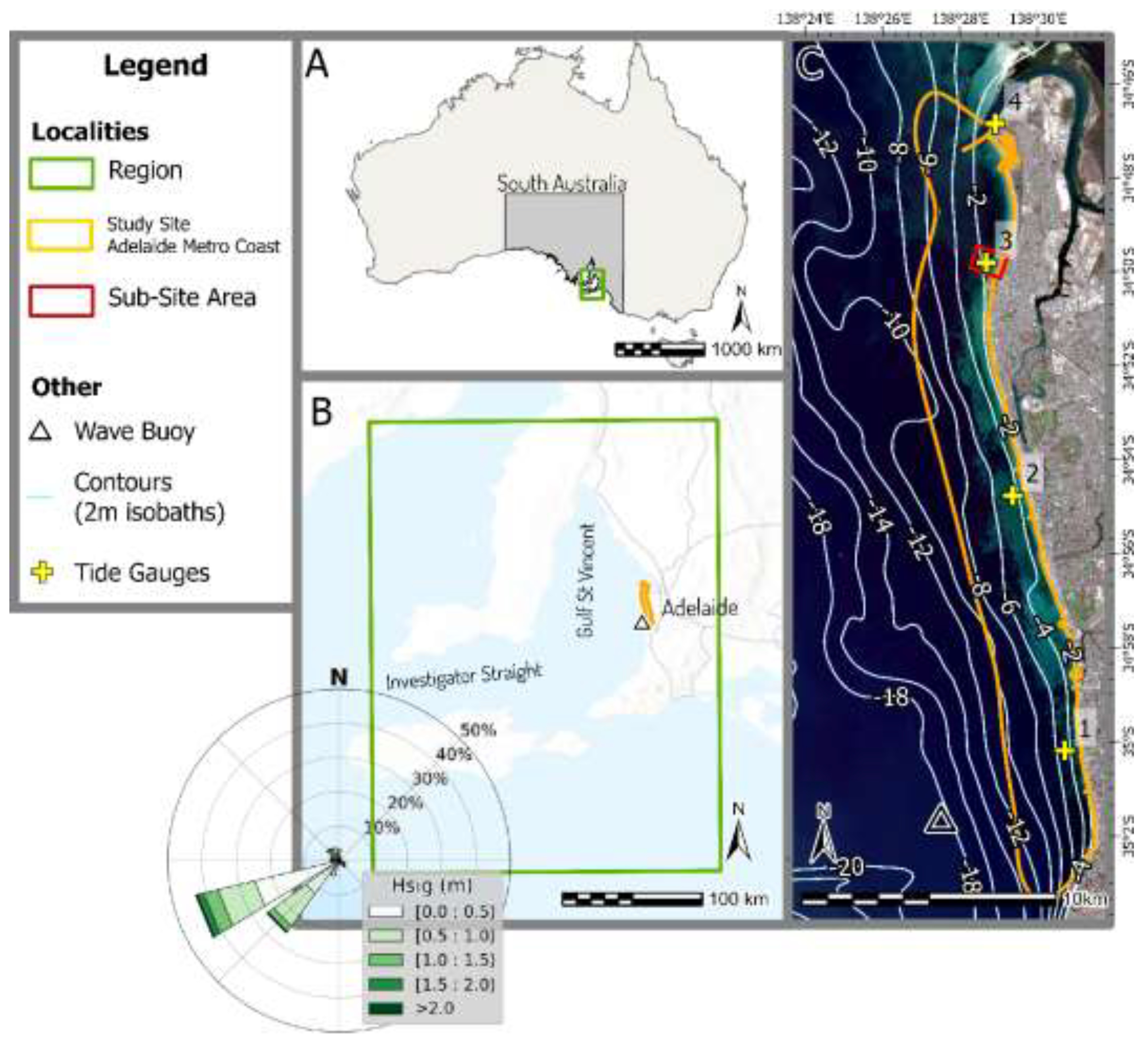
Figure 1.
Insert A depicts the study site’s regional setting within the Australian continent. Insert B displays the study site’s regional location, centred around the Gulf St Vincent along with a wave rose depiction of local swell conditions recorded over the past two years [27]. The broader study site’s spatial extent and bathymetric contours [28] are depicted in insert C. Also within insert C is a red rectangle displaying the location of the sub-site.
Multi-Resolution Optical Datasets
The study utilised wavelengths within the visible spectrum associated with satellite imagery from three distinct spaceborne multi-spectral instruments: Sentinel-2 (10m), PlanetScope SuperDove (3m), and Pléiades Neo (1.2m), offering unique spatial resolutions (pixel size) and spectral resolutions (number of bands and sampled portion of electromagnetic spectrum) (Table 1). In addition to selection based upon unique spatial and spectral resolutions, these satellites were chosen in part due to cost and the availability of archival imagery simultaneous with in situ data collection (Section 2.3). Sentinel-2 and PlanetScope SuperDove satellite imagery were obtained freely from Copernicus Browser and Planet Explorer archives respectively; in the case of the PlanetScope SuperDove, this data is only free of charge with an education and research license. Pleiades Neo imagery was obtained from AirBus through a tasked capture, with a reduced cost for research purposes. Further sensor technical details are provided in Appendix A.
To obtain the best quality imagery the following criteria were considered:
- The prevalence of cloud cover within the imagery.
- The date of image capture relative to in situ data collection (16th of January 2024 – see Section 2.3).
- Visible effects of sunglint over water.
- Visible effects of sea state.
- Visible effects of turbidity.
Considering the above criteria, an optimal multi-spectral image from each satellite provider was chosen, the details of which are listed in Table 2. These three multi-spectral images were collected within twelve minutes, ensuring minimal variability in environmental conditions. To facilitate fair comparison, each image was obtained at an equivalent surface reflectance level. All datasets were then reprojected to the Geocentric Datum of Australia 2020 (GDA2020) with a Universal Transverse Mercator (UTM) projection centred around zone 54 south.
Georectification
Satellite imagery underwent an assessment for spatial misalignment and was georectified accordingly. Initially, Pleiades Neo imagery was georectified using discernible points within the imagery that were surveyed using RTK GNSS, ensuring a precise georectification. Control points were confined to the land and kept level with the ground to mitigate errors associated with relief displacement. Consequently, the spatial distribution of control points could not be evenly spread across both the x and y extents. To prevent image distortion, a first-order polynomial (affine) transformation was applied using nearest neighbour resampling thus maintaining the original radiometric properties of the satellite imagery. The georectified Pleiades Neo image was then utilised as the 'truth' for an image-to-image first-order polynomial (affine) transformation of remaining multi-spectral images. The total RMSE on the x and y axes are reported in Table 3.
Coastal Water Separation
To isolate only marine inundated nearshore areas within the study area for analysis, pixels containing water were identified according to the normalised differenced water index (NDWI), as shown in Eq. 2, where and refer to display numbers in the green and near-infrared spectral bands, respectively. This was developed based on the Pleiades Neo imagery. A histogram thresholding algorithm was used to separate classes whilst maximising inter-class variance [29].
Sunglint Correction
The Hedley et al. (2005) method was employed to reduce sunglint (Eq. 3). This technique assumes that in deep water, near-infrared electromagnetic energy ) is almost completely absorbed throughout downwelling and upwelling passage in the water column. Consequently, the reflectance recorded in a deep-water region using the NIR band should ideally match the minimum value within that area . Any deviation from this minimum value serves as an indicator of the extent to which sunglint affects the reflectance in the visible bands . Following this assumption, the visible band can be corrected by determining the slope of a linear regression between the NIR and each visible band . Hence, the value for visible bands and the NIR band can be adjusted to match the minimum recorded NIR value observed over deep water [30].
SoNAR and LiDAR Bathymetry Data
The Department for Environment and Water collected twenty-nine sound navigation and ranging (SoNAR) profiles extending 1.5km from the shore at approximately 1km intervals along the metropolitan coast between December 2023 and January 2024 (Figure 2). In shallow waters, elevation was measured using land wading with real-time kinematic (RTK) global navigation satellite system (GNSS) techniques. For deeper waters, a high-frequency single-beam SoNAR was utilised. The data was quoted as having an accuracy of +/-5cm [31]. Elevations were provided every 0.5m along each profile, in total 75,876 observations were provided.
In addition to this dataset, a bathymetric LiDAR survey was conducted on 16th of January 2024 within the designated sub-site region using the ‘TDOT 3 green laser system’. The survey collected 988,660 point observations with a point spacing of 0.09m. This data was then validated against the existing SoNAR profile within the sub-site area (Figure 1). Subsequently, three surfaces representing the top of seafloor were generated from the point cloud using the binning method with a maximum cell assignment and no void fill; each surface had different spatial resolutions to ensure the spatial resolution corresponded with each multi-spectral image. Critically, all ground truth elevations represent the top of benthic features, not the underlying seabed. Therefore, the in situ data is comparable with SDB outputs which measure water column depth above the reflecting bottom surface (e.g. the top of a benthic feature).
All calibration and validation data were converted from bathymetric measurements to depth at the time of image capture of all three satellite images using a tidal adjustment based upon the ‘OTPS TPXO 9’ global tide model [32] with a resolution of 1/30 of a degree (≈4km). The preceding iteration of the TPXO 9 model has been validated against tide gauges in Australia, demonstrating an RMSE <0.12m [33]. The modelled tide was given in relation to mean sea level and demonstrated a total tidal range of 2.4cm from the south to north of the study site at time of image capture.
To further validate the tidal model in the gulf environment four tide gauges were positioned at equal intervals along the coast (Figure 1). Of the four, one tide gauge is a permanent system operated by Flinders Ports Pty Ltd, the remaining three were temporarily deployed with ‘RBR virtuso3’ loggers. Tide gauge logging parameters can be seen in Table 4. The vertical position of local tide gauges was known, as their deployed location was surveyed along with cross-shore profiles and the distance between the seafloor and sensor fixed. Hence, tidal heights were provided in relation to the tidal datum Australian Height Datum (AHD). The datum surface passes through approximate mean sea level.
Study Design
Identification of the Optimal Combination of Variables
The variables under scrutiny included the empirical derivation technique utilised, the input multi-spectral satellite image, and spectral bands employed in the SDB derivation process. This study utilised two dominant empirical derivation techniques found in literature to optimise passive SDB techniques; including the multiband linear technique [34,35] and the band ratio technique [36].
Lyzenga developed a semi-empirical algorithm, namely the ‘multiband linear technique’ to derive depth (Eq. 4). The algorithm leverages the exponential nature of attenuation of light as described by the Beer-Lambert Law [13] and assumes a constant bottom reflection difference between two spectral bands across all albedo types at any given depth, hence, multiple bands are used correct for the influence of variable bottom albedo [34,35]. Depth (d) can then be empirically determined if in situ data is present within the imagery by deriving coefficients from linear regression, specifically the y-intercept (m1) and slope (m0). Where is the water-leaving radiance of the band (w m−2 µm−1 sr−1) and is the atmospherically/sunlight corrected radiance in optically deep water, n is the number of bands (two or more), and i is the number of data points.
Throughout the literature the use of only blue and green bands prevails [17,18,19]. For use within this study, water leaving radiance was substituted for scaled water leaving reflectance as was the nature of the data at the completion of image pre-processing; this substitution has also been performed successfully within literature [37].
Stumpf, Holderied, and Sinclair (2003) provided an alternative to the multiband linear technique known as the ‘band ratio technique’. The band ratio technique derives depth based upon a linear relationship between depth and the ratio of the natural logarithm of atmospherically/sunlight corrected water leaving reflectance () values from one band to another. This technique commonly uses the two bands that penetrate furthest into the water column [17]. As the depth increases, the reflectance of both bands decreases. However, the natural logarithm of the band with higher absorption (typically blue in coastal water) decreases faster than the natural logarithm of the band with lower absorption (typically green in coastal waters). Consequently, the ratio of green to blue will increase with increasing depths. Thus, the depth-induced change in the ratio far outweighs that caused by alterations in bottom albedo, hence different bottom albedos at a constant depth will still yield the same ratio [38]. The band ratio algorithm can be seen in Eq. 5.
RMSE was used as a metric to assess dataset quality, as is common practice within SDB literature [39]. A reduced RMSE implies a lesser fluctuation in errors between the actual and derived water depths, indicating a better-performing SDB derivation. The RMSE equation is given in Eq. 6. The variable denotes the ground truth value of sample i, represents the SDB estimated value for sample i, and n is the number of samples.
Determination of the optimal combination of variables was achieved by exhaustively deriving depth with every possible combination of these variables. In total, 109 SDB derivations with unique variable combinations were generated and their RMSE values recorded for assessment. The final optimised dataset equated to the method with the lowest RMSE.
Determination of the Impact of Spatial Resolution and Spectral Suitability upon Dataset Quality
The study extended beyond identifying the optimal variable combinations. Equally significant was deciphering how predictor variables (spatial resolution and the spectral suitability of the input bands) influence dataset quality (RMSE).
Spectral suitability was created in this study as a metric of both spectral resolution and the applicability of the spectral bands for use in coastal water, hence, preferencing the use of bands that penetrate furthest through the coastal water column. Specifically, spectral suitability incorporates the number of bands used (N), the average bandwidth (AvBw) (nm) of these bands, and the spectral distance (SpD) (nm) of a given band’s central wavelength (λi) (nm) from the optimal wavelength for light penetration in coastal water. The optimal wavelength for light penetration in coastal water is identified as between 520 and 580nm dependent upon local water quality parameters such as chlorophyll concentration, salinity and temperature [40], hence, the midpoint (550nm) was selected as optimum. Both SpD and AvBw are given in nanometres whilst N is dimensionless, therefore, all input coefficients were normalised between an infinitely small number and 1 where a number close to 0 indicates suitability and 1 un-suitability. To normalise SpD, the coefficient was divided by the largest possible spectral distance observed between all input bands’ central wavelength and the optimal wavelength for coastal water penetration; this value was given as Δλ (nm). Likewise, AvBw was normalised by dividing by Δλ. These normalised variables were summed together to rank the spectral suitability of the input bands. The equation is as follows (Eq. 7).
A series of candidate multiple linear regressions (MLRs) were developed using all available SDB derivations for each technique (24 observations for band ratio and 85 observations for multiband linear technique). An exhaustive amount of MLRs were generated based on every possible combination of predictor variables. These models were then ranked using Akaike’s Information Criterion (AIC) [41]. The AIC metric served as a crucial tool for the best model selection where more simplistic and probabilistic models have lower AIC scores, and less parsimonious models demonstrate larger scores. It penalised overly complex models, thus mitigating the risk of fitting the model to data noise. Furthermore, AIC prioritised probabilistic models in accordance with each model’s maximum likelihood. AIC is given in Eq. 8 where ι is the maximum likelihood and k the number of parameters in the model including the y-intercept.
When comparing models, an evidence ratio (ER) was generated to quantitatively compare which model is more parsimonious than another. The evidence ratio formula is given in Eq. 9.
Validation of the Optimised SDB Method
Lastly, using the optimised SDB technique and the output equation of the line for calibration, a bathymetric surface was generated for validation across the entire study site using all available SoNAR data and remaining bathymetric LiDAR data unused in the calibration phase. Importantly, the in situ data is predominately outside the sub-site to avoid validating the model in an identical environment to the sub-site. This is essential to ensure the model's robustness and applicability beyond the sub-site boundaries. The dataset quality metric RMSE was observed, and residual errors analysed as a function of environmentally dependent variables such as observed depth and bottom type.
A summary of the complete study design has been provided in Appendix B.
Data Analysis
Identification of the Optimal Combination of Variables
The pre-processed multi-spectral images, along with the tidally corrected high-resolution bathymetric data obtained within the sub-site were input into the Jupyter Notebooks Python environment (script provided within supplementary material). 109 SDB derivations (listed in Appendix C) were then performed using exhaustive band combinations upon all satellite images using the multiband linear technique and the band ratio technique within the smaller sub-site.
Each derivation was calibrated and validated utilising in situ data within the sub-site. Calibration and validation data was predominantly derived with bathymetric LiDAR but also included the SoNAR profile 200004 which intersects the bathymetric LiDAR data (Figure 2). Observations were rasterised at the same resolution as the input bands, each cell value was assigned by the mean value of all observations within a given cell. The in situ data extended from 0m to 7.5m water depth at time of image capture and had a bi-modal distribution (Figure 3), hence, calibration and validation was underrepresented at the depth extremities. Half of the available bathymetric LiDAR data and SoNAR profiles were used as calibration, the remaining half were utilised as validation data.
Bottom type was classified at the pixel level for every validation observation to analyse the impact of bottom types upon data quality. Bottom type information was derived from the input Pleiades Neo imagery using iterative self-organising (ISO) cluster unsupervised classification. Two classes ‘sand’ and ‘non-sand’ bottom types were identified; ‘non-sand’ pixels were identified as lower albedo features. These low albedo features are thought to be primarily seagrass meadows [42]. The classification exhibited good agreement as demonstrated with an overall accuracy of 91.5% and a kappa value of 0.804. The output bottom type raster was resampled using nearest neighbour resampling to match the resolution of Sentinel-2 and PlanetScope Super Dove bands. Calibration data utilised within the sub-site was represented by the ‘sand’ bottom type more than the ‘non sand’ class accounting for 74% of the data.
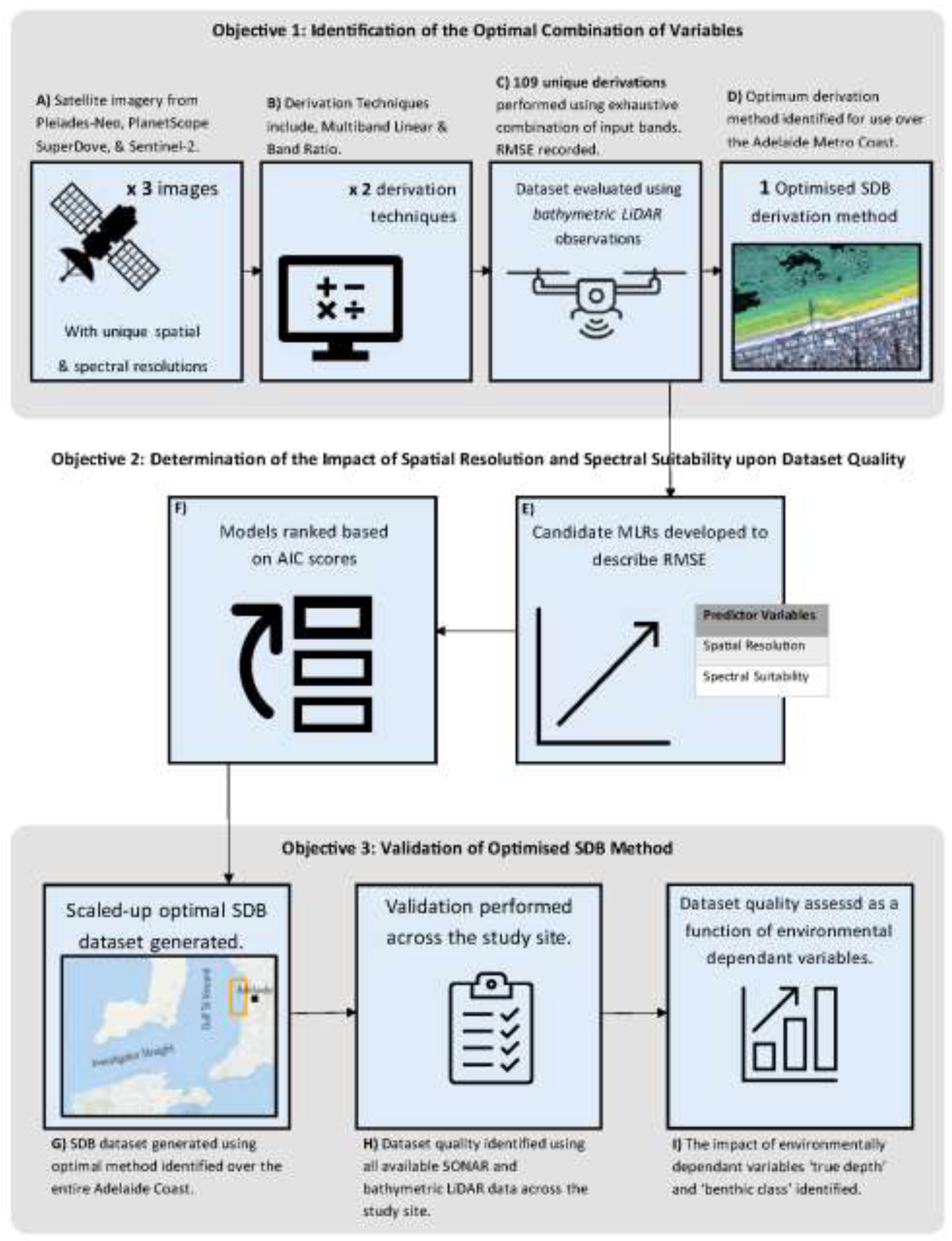
An overview of methods used to generate and assess the quality of SDB datasets is provided in Figure 4.
Determination of the Impact of Spatial Resolution and Spectral Suitability Upon Dataset Quality
For each of the 109 SDB derivations performed the critical variables thought to impact dataset quality were recorded, including the impact of spatial resolution (pixel size - m) and input spectral band suitability, allowing for the impact of these variables upon dataset quality to be statistically explored. The impact of spatial resolution and spectral suitability upon data quality (RMSE) was then modelled for each derivation technique using MLR. The following models were ranked based on their AIC scores:
- RMSE (m) ~ (Pixel Size (m)) and (Spectral Suitability)
- RMSE (m) ~ (Pixel Size (m))
- RMSE (m) ~ (Spectral Suitability)
Candidate models were ranked based on their parsimony as a function of their AIC and then compared based on their output ER. The Python script utilised to generate MLRs, and AIC scores is provided in the supplementary material
- 1.
- 2. Validation of the Optimised SDB Methods
The derivation process outlined in section 2.5.1 was again utilised to perform the optimal SDB derivation method across the entire study site. The in situ data used for accuracy assessment was equally distributed across the entire site along the horizontal axes. In situ data included bathymetric sub-site validation data (unused in the calibration phase), as well as all 28 remaining SoNAR profiles (Figure 2). In total, there were 13368 validation observations. Both the output SDB dataset and the validation data were restricted to an operational depth range determined based on model performance (per the results of section 3.3). Depth observations used in the validation of the optimal method throughout the study site were well distributed from a frequency perspective (Figure 5). The bottom type was overrepresented by the ‘sand’ bottom type (70%).
Furthermore, dataset quality checks were performed to understand the influence of environmental factors true depth, and bottom type upon dataset quality. This was achieved by assessing the mean average error in depths of 1m intervals and according to their ‘sand’ and ‘non-sand’ classes.
Results
Sunglint Correction
A before and after sunglint correction comparison over visibly affected water is presented in Figure 6.
Notably, in shallow water (≈<0.5m water depth) a weak NIR bottom reflectance was observed, hence the sunglint correction led to the reduction of digital numbers (DN) in visible bands regardless of the presence of sunglint. Regions affected by NIR bottom reflectance were identified in the Pleiades Neo imagery (Figure 7).
In Situ Data Agreement and Tidal Model Validation
In situ data used for calibration and validation was quality assured. Comparison between SoNAR and LiDAR derived measurements where overlap was present yielded an RMSE of 0.064m, indicating strong alignment between the datasets. A profile comparison is presented in Figure 8.
Additionally, validation of the tidal model with local tidal measurements demonstrated a positive linear relationship with good correlation (0.97 and 0.73 R2 respectively), and a similar gradient when plotted as a function of chainage from south to north along the coast (Figure 9). The TPXO 9 model had an RMSE of 0.04m when validated against the local tide gauges.
Identification of the Optimal Combination of Variables
Of the 109 unique SDB derivations, each utilising different band combinations, satellite imagery, and derivation techniques, the multiband linear technique consistently outperformed the band ratio technique. Analysis of each SDB derivation’s RMSE revealed a pattern that SDB derivations using the multiband linear technique were both more accurate and displayed lesser variance (interquartile range) compared to the band ratio technique (Figure 10). Particularly noteworthy was the performance of the multiband linear technique with PlanetScope SuperDove imagery, where it showcased the lowest mean RMSE values and interquartile range compared to all other combinations of input satellite image and derivation technique
The optimal combination of satellite imagery, input bands, and derivation technique was achieved using PlanetScope SuperDove imagery, input green-alt (535nm), green (570nm), and yellow bands (610nm), and using the multiband linear technique. This attained an RMSE of 0.408 (Figure 11). The following 9 of the top performing 10 SDB derivations all were performed using the multiband linear technique with input PlanetScope SuperDove imagery and slight variations of input bands always including at least two bands from the optimum band combination (Appendix C). The best SDB derivation using the band ratio technique was obtained using Pleiades Neo green and blue bands and ranked 69th overall (Appendix C). The optimised dataset displayed a high degree of linearity (R2 = 0.94) and performed well in depths greater than 1m and less than 5m (Figure 11), outside of this range SDB depth estimations deviated from the linear relationship, hence, SDB estimations in these regions were routinely shallow. The divergence between observed depth and derived depth in these regions can be seen when the two datasets’ cross-shore profiles are contrasted (Figure 12). Hence, in water >5m deep the optimal SDB derivation is not an effective estimation of water depth.
Determination of the Impact of Spatial Resolution and Spectral Suitability on Dataset Quality
The study found no correlation between spectral suitability and spatial resolution with dataset quality when analysing the RMSE from all SDB derivations using the band ratio technique. However, the best-performing technique, multiband linear technique, did show correlations with these variables (Table 5). Specifically, there was a weak positive correlation (R² = 0.31) between pixel size and RMSE and a moderate positive correlation (R² = 0.49) between spectral suitability and RMSE. The MLR model was strongest when both variables were used as predictors, with an R² of 0.78. The study determined that smaller pixel sizes and spectral suitability values resulted in reduced RMSE, indicating that as input bands become more suitable and spatial resolution is increased dataset quality is improved (Figure 13).
Furthermore, the AIC scores indicate that for the MLR technique, the model incorporating both spectral suitability and pixel size not only explains the greater variance but is also more parsimonious than either model using either variable alone (Table 5). The ER between the optimal model and the next best performing model was determined to be 7.26×10¹⁵, hence the model is 7.26×10¹⁵ times more parsimonious. Therefore, when both spectral suitability and spatial resolution are considered as predictors of dataset quality they provide an overwhelmingly more robust estimation of the drivers for dataset quality than other candidate models despite its increased complexity.
Validation of the Optimised SDB Method
The optimised dataset was validated across the broader study site in depths between 0.5m and 5m, as the optimised derivation proved unsuitable beyond these limits (Section 3.3); hence no estimation of depth was made beyond 5m and less than 0.5m water depth. Overall accuracy decreased compared to the sub-site validation, with RMSE increasing from 0.41m to 0.51m (Figure 14). Notably, in regions with depths greater than 4m, the correlation between satellite-derived depth and in situ depth observations weakened, making depth estimation less reliable. The variability observed in Figure 14 is largely attributed to environmental factors, particularly, heterogeneous bottom albedo within the study site. The grouping of observations within the dashed box are likely associated with a discrete, higher-albedo sandy substrate in the south of the site, highlighting the limitations of empirical methods in accounting for such environmental heterogeneity.
The output bathymetric raster is shown in Figure 15, along with validation cross-shore profiles distributed throughout the north, central, and south of the study site. These cross-shore profiles contain varying amounts of ‘non-sand’ pixels. The northern profile (200001) contains only ‘sand’ pixels. In this singular class, the optimised derivation successfully identifies four defined bars and troughs in the nearshore. However, at greater depths, the SDB dataset routinely diverges from true depth, underestimating depth by 1m at 5m water depth.
The following two profiles, situated in the central and southern parts of the study site, show the impact of ‘non-sand’ pixels on estimated depth. In these regions corresponding with regions seaward of the landward extent of seagrass, depth estimates frequently switch from underestimating to overestimating, often by 50cm, and in the case of profile 200021, by upwards of 2m at a true depth of 3.5m. Thus, the use of multiple bands for depth estimation does not appear to account for changes in albedo as a function of bottom type, as suggested in the literature [6,8,34].
Further investigation into the impact of environmental factors on the optimised derivation accuracy across the study site confirmed the deepening effect over ‘non-sand’ pixels and the inverse over ‘sand’ pixels (Figure 16). On average low albedo ‘non-sand’ pixel depth estimates were 19cm too deep and ‘sand’ pixels 15cm too shallow. Furthermore, it was observed that the total mean average error increased beyond observed depths of 2m; before reducing in depths >4m; however, this reduction in depths greater than 5m is unrealistic considering the output SDB dataset was restricted to 5m, therefore depth estimates over ‘non-sand’ (the dominant bottom type at this depth) were restricted from overestimating depth.
Discussion
Identification of the Optimal Combination of Variables
The study aimed to determine an optimal derivation method in an optically shallow, mixed bottom, low wave energy coastal environment, based on a selection of the best-performing combination of three critical variables; the input satellite imagery (Sentinel-2, Pleiades Neo & PlanetScope SuperDove); the input spectral bands utilised in the SDB derivation; and the empirical derivation technique itself (multiband linear and band ratio). This was in response to a need to expand on existing literature which is limited in number and scope, necessitating further investigation to fully leverage recent advancements in improved spatial and spectral resolution of low-earth orbiting satellites [16]. For example, recent work by Evagorou (2022) made significant progress in determining an optimised derivation method but overlooked the potential of the superior PlanetScope SuperDove constellation, warranting further investigation.
The investigation into identifying the optimal combination of variables yielded three major insights. Firstly, after analysing 109 unique SDB derivations, encompassing various band combinations, satellite imagery, and derivation techniques, it became evident that the multiband linear technique consistently outperformed the band ratio technique. This superior performance is evident in Figure 10, where derivations performed with the multiband linear technique exhibited reduced mean RMSE, and inter-quartile variance compared to the band ratio technique. Secondarily, the performance of the multiband linear technique when applied to PlanetScope SuperDove imagery consistently showcased the lowest mean RMSE values among all potential imagery and derivation technique combinations (Figure 10 & Appendix C). Lastly, the optimal derivation method was determined to involve the use of PlanetScope SuperDove imagery with input bands green-alt, green, and yellow, utilising the multiband linear technique. This achieved an R² value of 0.94 and an RMSE of 0.41m when compared to high-resolution bathymetric LiDAR observations within the sub-site from which it was calibrated, as shown in Figure 11. However, despite its accuracy within depths ranging from greater than 0.5m to less than 5m, the dataset exhibited divergence from true depth at depths outside of this range (Figures 11 & 12).
The results of a similar empirical approach by Evagorou et al. [6] contrast with the findings of this study. Specifically, Evagorou et al. [6] found that the band ratio technique outperformed the multiband linear technique at depths of 0-10m when applied to WorldView-2 and Sentinel-2 imagery, with RMSE values of 1.01m and 1.06m, respectively. Although the multiband linear technique performed better than the band ratio technique with 4-band PlanetScope imagery, it recorded the poorest RMSE (1.08m) among all input satellite imagery. The author's analysis of true depth's impact on mean residual error revealed that the multiband linear technique outperformed the band ratio technique at depths less than 4m. They observed that at depths greater than 4m, the band ratio technique routinely outperformed the multiband linear technique. Evagorou et al. [6] determined that the optimised derivation was achieved using only green and blue bands.
The discrepancy between studies regarding the determined optimal combination of variables may be due to a limitation of this study, regarding the equal vertical distribution of in situ bathymetric data within the sub-site. In situ data was spread between 0m to 7.5m water depth at time of image capture, however, the bi-modal distribution of depth within this range meant depths towards the extremities of this range were underrepresented in calibration and validation (Figure 3). Notably, in depths less than 0.5m and greater than 5m the presence of in situ data exponentially declines. Based on Evagorou et al. [6] analysis of the impact of depth across all combinations of derivation techniques and satellite images, this bi-modal distribution of in situ data may have advantaged the multiband linear technique. Therefore, the findings of this study should not be thought relevant in depths greater than 5m and less than 0.5m water depth.
Determination of the Impact of Spatial Resolution and Spectral Suitability upon Dataset Quality
Furthermore, the research aimed to describe how spatial resolution and the spectral suitability of the input bands (given the coastal application) influence dataset quality (RMSE). Despite traditional practices favouring the use of green and blue bands due to their superior penetration into the water column [17,18,19], recent observations suggest the potential benefits of hyper-spectral data for improving accuracy, particularly when employed with machine learning algorithms [20,21]. However, it remains uncertain whether such enhancements apply to SDB derivations performed with traditional techniques. Furthermore, Evagorou et al. [6] identified that the impact of spatial resolution of satellite imagery on SDB quality should be a subject of future work. Therefore, this study sought to address these uncertainties and provide insights into the impact of spatial and spectral characteristics of input bands on dataset quality, thus advancing our understanding of SDB derivation techniques in coastal environments.
The relationship between predictor variables (pixel size (m) and input spectral band suitability), and the response variable (SDB dataset RMSE (m)) was evaluated based on the results of 109 SDB derivations generated within the sub-site (Table 5). While no correlation was found between predictor variables (spectral suitability and pixel size) and RMSE using the band ratio technique, MLRs revealed correlations between both spectral suitability and pixel size with RMSE in SDB derivations obtained with the multiband linear technique. Specifically, there was a weak positive correlation between pixel size and RMSE, whereas a moderate positive correlation was observed between spectral suitability and RMSE, indicating that the spectral characteristics of input bands had a more pronounced influence on dataset quality than pixel size. The MLR model incorporating both predictor variables exhibited the strongest overall performance, explaining 78% of the variance in dataset quality. Furthermore, despite the increase in this model’s complexity, AIC model ranking determined this model to also be more parsimonious.
The finding suggest that spectral suitability could function as a theoretical means of band selection, however, the metric is limited by the assumption that optimum band selection will not change with bottom type. The impact of which has not been explored as detailed bottom type was not resolved beyond simply ‘sand’ and ‘non-sand’. To the best of the authors' knowledge, an a-priori mechanism for optimal band selection has not yet been published. The spectral suitability metric (Eq. 7), while a preliminary solution, provides an initial conceptual framework. Future studies should focus on refining the metric to account for a wider range of bottom types and site-specific water quality conditions.
Furthermore, the findings provide valuable insights into the factors that enhance the accuracy of SDB datasets in optically shallow, mixed bottom, low wave energy coastal environments. The superior performance of the multiband linear technique can be attributed to its ability to incorporate more spectral information. Furthermore, this ability to leverage multiple bands is particularly advantageous when using high-resolution imagery from satellites like PlanetScope SuperDove, which features narrower bandwidths and increased sampling near the optimal wavelengths for water penetration, specifically the green-alt, green, and yellow bands. Conversely, Sentinel-2's relatively wider bandwidths, fewer sampled wavelengths in the visible range, and larger pixel sizes limit its effectiveness for SDB in the studied environment.
Moreover, these findings suggest that hyper-spectral sensors, when used in conjunction with the multiband linear technique, may yield more accurate SDB outputs. Their capability to sample the electromagnetic spectrum at high resolution renders them highly suitable for nearshore applications. For example, the EnMap satellite sensor has 6.5nm spectral sampling intervals and an average bandwidth of 8.1nm within the visible spectrum range; and pixel sizes of 30m [43]. Theoretically, if the input bands utilised cover the spectral range identified as optimal (Section 3.3) (513 – 620nm), resulting in a total of 16 bands, the spectral suitability is calculated as 0.37, which is 57% more suitable than the spectral suitability of the optimal combination of bands (Appendix C). However, due to the inflated pixel size, the model-inferred RMSE for this theoretical SDB derivation is 1.17m (Equation 10); assuming fixed weather-dependent variables such as turbidity, sea state, and sunglint. Despite the modelled inflation of RMSE using EnMap input bands, the stark improvement in spectral suitability and the observed moderate correlation between the predictor variable and RMSE (Table 5) warrants further comparison of multi-spectral and hyper-spectral derived SDB products.
Validation of the Optimised SDB Method
Further validation of the optimised methods on the broader study site between depths of 0.5 and 5m revealed that the optimal derivation method performed well along the broader coastline. The achieved RMSE of 0.51m surpasses most empirical studies within literature, which similarly estimated depths using optical satellite data in mixed bottom type environments and in depths less than 10m. Most of these studies report RMS errors of no less than 0.8m ([6,44,45,46]), Few studies achieve the accuracy seen in this study without the use of machine learning. One such exception used PlanetScope data and reported an RMSE of 0.32m [47].
Whilst the overall dataset quality metrics were positive, problems were encountered accounting for different bottom types and their ranging albedos impact upon depth observations. On average, low albedo ‘non-sand’ pixels depth estimates were 19cm too deep and ‘sand’ pixels 15cm too shallow (Figure 16), indicating that the multiband linear technique is influenced by variable bottom albedo. This bias error is due to low albedo features reflecting less light energy due to absorption, similar to the effect that increased passage through the water column would incur [36]. The nature of calibration to variant albedo bottom types renders the equation of the line as the best solution to explain depth estimation variance yet not providing correct estimates for the unique bottom types.
Regarding the impact of true depth on SDB dataset quality, this study observed that total mean average error increased beyond observed depths of 2m; before reducing in depths >4m (Figure 17); although, this reduction in depths greater than 4m is unrealistic considering the output SDB dataset was restricted to 5m. Therefore, depth estimates over ‘non-sand’ (the dominant bottom type at this depth) were restricted from overestimating depth. Despite this finding the actual influence of increasing depth upon SDB dataset quality remains unknown due to the spatially correlated nature of true depth and bottom type. The dominant ‘non-sand’ bottom type within the study site is seagrass [42]. Seagrass has specific wave energy limitations for survival, resulting in a defined landward limit of seagrass growth, in part constrained by depth [48]. Within the study site seagrass was present in depths greater than 2m at time of image capture (Figure 16) and at greater densities in deeper water. The correlation between bottom types with true depth confounds the influence of true depth upon SDB dataset quality. A potential solution to this problem would be to construct independent bottom type regressions for calibration, prior to mosaicing each bottom type’s output bathymetric raster together for validation. This process has been demonstrated to improve RMSE from 1.31m to 1.16m when utilising empirical derivation techniques within a coral atoll environment [49]. This bottom type correction would not only account for the confounding impact of variable bottom albedo upon SDB dataset quality, but also enable the influence of increasing depth upon SDB dataset quality to be better understood.
Poor performance in shallow water (depths less than 0.5m) was demonstrated by a deviation between the estimated depth and the linear relationship with true depth (Figure 11). The cause of this deviation from the ln-linear relationship is uncertain; however, this study postulates that the source of this anomaly is introduced during the sunglint correction of visible bands. The Hedley et al. [30] sunglint removal algorithm adjusts each visible band based upon the amount of NIR reflectance thought to be attributed to sunglint, corresponding with the difference between the value of the NIR band of a pixel (RNIR) and the minimum NIR value (MINNIR) (Equation 3). However, as the MINNIR value is attributed to both sunglint and bottom reflectance in shallow water, the visible bands DN’s are being independently overly corrected by a factor of the slope of the linear relationship between each visible band and the NIR band (bi),resulting in optical change in colour and confounding depth estimates. Regions determined to contain NIR bottom reflectance were identified (Section 3.1). It was determined that in depths at time of image capture of less than 0.88m the majority of pixel observations were affected by NIR bottom reflectance (Figure 17). Furthermore, in increasingly shallower depths pixels are more affected by NIR bottom reflectance. For these reasons, it is proposed that poor SDB dataset quality in shallow water is attributed to the use of the Hedley et al. [30] sunglint correction method in regions where NIR bottom reflectance is present. Alternative methods for sunglint correction in shallow water should be sought.
Despite the identified limitations in SDB depth estimation as a function of variable bottom albedo and poor performance in shallow water, the identified optimised SDB method does enhance the capability for coastal practitioners to capture cost-effective, spatially and temporally extensive bathymetric grids with improved accuracy along the Adelaide Metropolitan Coast and in similar coastal environments between depths between 0.5 to 5m, such as protected gulfs. This, in turn, increases the capacity to monitor coastal sedimentary responses to sea level rise, aiding in the management of beach amenities, coastal infrastructure, and coastal ecology. However, caution should be taken when attempting to use calibration coefficients identified in this study to derive bathymetric datasets based on satellite imagery, as changes in environmental conditions at the time of image capture, such as, turbidity, high sea-states, sea-surface reflectance, and atmospheric scattering will impact the rate of light attenuation [14]; necessitating another calibration.
In addition to future research proposed into the capability of hyper-spectral satellites for depth estimation along the Adelaide Metropolitan Coast, future research should also incorporate the use of machine learning algorithms along the coast for SDB depth estimation. These algorithms can identify variability in environmental conditions using spectral indices and classification, hence, the technique may be a robust solution in heterogeneous environments [50]. Additionally, machine learning models, once trained using extensive in situ measurements encompassing diverse environmental conditions, can be deployed in differing locations, adapting to unique bottom types and water quality conditions. Conclusions
The study underscored the increased performance of the multiband linear technique in bathymetric estimation compared to the band ratio technique, particularly when applied to PlanetScope SuperDove imagery. This technique yielded the lowest RMSE values with input bands green-alt, green, and yellow.
Furthermore, the study emphasised the significance of both spatial resolution and spectral suitability in influencing dataset quality, as demonstrated by the most parsimonious model for estimating dataset quality (RMSE), which incorporates both predictor variables (spatial resolution and spectral suitability of input bands). The findings suggest that incorporating more spectral bands, especially those with narrower bandwidths and increased sampling near optimal wavelengths for water penetration, enhances empirical SDB accuracy. The research further indicates the potential benefits of hyper-spectral sensors, which, despite larger pixel sizes, offer extremely high spectral resolution that can improve bathymetric estimates.
Despite these advancements, validation of the optimised SDB dataset across diverse conditions within the broader study site revealed limitations in relation to shallow water (<0.5m) and challenges posed by variable bottom albedo. The findings suggest the need for alternative sunglint correction methods in shallow water and independent calibration of bottom types. The optimised SDB method identified in this study enhances the capability of coastal practitioners to capture cost-effective, spatially, and temporally extensive bathymetric datasets, thereby improving the monitoring and management of coastal environments. Future research should focus on integrating hyper-spectral data and machine learning techniques to further improve SDB methods and extend their applicability in diverse coastal conditions.
Author Contributions
Conceptualization, J.D.; methodology, J.D., D.B.; validation, J.D., G.M.d.S.; formal analysis, J.D.; data curation, J.D., G.M.d.S.; writing—original draft preparation, J.D.; writing—review and editing, J.D., D.B., G.M.d.S., P.H.; visualisation, J.D.; supervision, D.B., G.M.d.S., P.H.; project administration, J.D., D.B.; funding acquisition, J.D., D.B., P.H.
Funding
This research was funded by The Coast Protection Board, grant number DEW-DO027147 and by the Flinders University Innovation Partnership Seed Grant, grant number CNTR0015598.
Data Availability Statement
Multi-spectral satellite imagery is available online, in the case of the Pleiades Neo imagery it must be purchased from AirBus. Details required for purchase can be found in section 2.2 of this article. Calibration and validation datasets can likely be shared upon request pending approval from the Department for Environment and Water. For access to scripts used throughout the project please refer to the links within the supplementary materials.
Acknowledgments
The authors thank all members of the BEADS lab/Geospatial unit, particularly, Robert Keane and Claire Moore who proved invaluable in the bathymetric LiDAR data collection process. A special thanks to Marcio DaSilva for his ongoing support to the authors.
The authors express gratitude to the Department for Environment and Water’s Hydrographic Survey team for their provision of data, support with fieldwork, and interest in the project. Without their assistance the project’s findings would be less robust.
Conflicts of Interest
The authors declare no conflicts of interest.
Appendix A - Sensor Comparison for Sentinel-2, PlanetScope SuperDove, and Pleiades Neo
| Parameter | Sentinel-2 | PlanetScope SuperDove | Pleiades Neo |
| Pixel Size | 10–60 m | 3 m | 1.2 (30 cm for Panchromatic) |
| Swath Width | 290 km | 25 km | 14 km |
| Spectral Range | 443–2190 nm (Visible, NIR, SWIR) | 400–860 nm (Visible, NIR) | 430–950 nm (Visible, NIR) |
| Number of Bands | 13 | 8 | 6 |
| Temporal Resolution | 5 days | Daily (subject to constellation) | Daily (subject to tasking) |
| Radiometric Depth | 12-bit | 12-bit | 12-bit |
| Imaging Mode | Push-broom | Push-broom | Push-broom |
| Number of Satellites in Constellation | 2 | ~200 SuperDove | 4 |
| Launch Year | Sentinel-2A: 2015, Sentinel-2B: 2017 | 2020 | 2021–2022 |
| Data Accessibility | Copernicus Browser | Planet Explorer | Airbus |
| Cost | Free | Varies by license | High |
Appendix B - Summary of Study Design
Appendix C – Derivations Ranked by their RMSE Values
| ID | Derivation Technique | Input Imagery | Bands | R2 | RMSE | Mean Residual (Sand) | Mean Residual (Non-Sand) |
| 1 | Multiband Linear Method | PlanetScope SuperDove | Green(I), Green, Yellow | 0.936 | 0.408 | 0.009 | -0.029 |
| 2 | Multiband Linear Method | PlanetScope SuperDove | Green, Yellow | 0.934 | 0.415 | 0.033 | -0.095 |
| 3 | Multiband Linear Method | PlanetScope SuperDove | Green(I), Green, Red | 0.933 | 0.415 | 0.020 | -0.058 |
| 4 | Multiband Linear Method | PlanetScope SuperDove | Blue, Green(I), Green, Yellow | 0.932 | 0.418 | 0.007 | -0.023 |
| 5 | Multiband Linear Method | PlanetScope SuperDove | Blue, Green, Yellow | 0.932 | 0.420 | 0.022 | -0.064 |
| 6 | Multiband Linear Method | PlanetScope SuperDove | Blue, Green(I), Green, Red | 0.931 | 0.423 | 0.015 | -0.045 |
| 7 | Multiband Linear Method | PlanetScope SuperDove | Blue, Green(I), Green, Yellow, Red | 0.930 | 0.424 | 0.036 | -0.102 |
| 8 | Multiband Linear Method | PlanetScope SuperDove | Green(I), Green, Yellow, Red | 0.930 | 0.426 | 0.045 | -0.128 |
| 9 | Multiband Linear Method | PlanetScope SuperDove | Green(I), Yellow | 0.928 | 0.431 | 0.041 | -0.116 |
| 10 | Multiband Linear Method | PlanetScope SuperDove | Blue, Green(I), Yellow | 0.928 | 0.433 | 0.028 | -0.079 |
| 11 | Multiband Linear Method | PlanetScope SuperDove | Blue, Green, Red | 0.927 | 0.435 | 0.036 | -0.101 |
| 12 | Multiband Linear Method | PlanetScope SuperDove | Deep Blue, Blue, Green(I), Green, Yellow | 0.925 | 0.441 | 0.022 | -0.060 |
| 13 | Multiband Linear Method | PlanetScope SuperDove | Green, Red | 0.924 | 0.442 | 0.055 | -0.155 |
| 14 | Multiband Linear Method | PlanetScope SuperDove | Deep Blue, Blue, Green(I), Green, Yellow, Red | 0.924 | 0.442 | 0.044 | -0.122 |
| 15 | Multiband Linear Method | PlanetScope SuperDove | Deep Blue, Green(I), Green, Yellow | 0.924 | 0.442 | 0.027 | -0.075 |
| 16 | Multiband Linear Method | PlanetScope SuperDove | Blue, Green, Yellow, Red | 0.924 | 0.443 | 0.058 | -0.163 |
| 17 | Multiband Linear Method | PlanetScope SuperDove | Deep Blue, Blue, Green(I), Green, Red | 0.923 | 0.447 | 0.029 | -0.080 |
| 18 | Multiband Linear Method | PlanetScope SuperDove | Deep Blue, Green(I), Green, Yellow, Red | 0.922 | 0.448 | 0.054 | -0.148 |
| 19 | Multiband Linear Method | PlanetScope SuperDove | Green | 0.922 | 0.449 | -0.032 | 0.084 |
| 20 | Multiband Linear Method | PlanetScope SuperDove | Blue, Green(I), Red | 0.922 | 0.450 | 0.043 | -0.120 |
| 21 | Multiband Linear Method | PlanetScope SuperDove | Deep Blue, Green(I), Green, Red | 0.921 | 0.451 | 0.038 | -0.102 |
| 22 | Multiband Linear Method | PlanetScope SuperDove | Green(I), Green | 0.921 | 0.452 | -0.030 | 0.080 |
| 23 | Multiband Linear Method | PlanetScope SuperDove | Blue, Green(I), Yellow, Red | 0.920 | 0.454 | 0.063 | -0.177 |
| 24 | Multiband Linear Method | PlanetScope SuperDove | Deep Blue, Blue, Green, Yellow | 0.920 | 0.455 | 0.038 | -0.107 |
| 25 | Multiband Linear Method | PlanetScope SuperDove | Blue, Green(I), Green | 0.920 | 0.455 | -0.021 | 0.054 |
| 26 | Multiband Linear Method | PlanetScope SuperDove | Blue, Green | 0.920 | 0.456 | -0.017 | 0.042 |
| 27 | Multiband Linear Method | PlanetScope SuperDove | Green, Yellow, Red | 0.918 | 0.461 | 0.079 | -0.221 |
| 28 | Multiband Linear Method | PlanetScope SuperDove | Deep Blue, Blue, Green, Yellow, Red | 0.917 | 0.463 | 0.064 | -0.178 |
| 29 | Multiband Linear Method | PlanetScope SuperDove | Blue, Yellow | 0.917 | 0.465 | 0.065 | -0.184 |
| 30 | Multiband Linear Method | PlanetScope SuperDove | Green(I), Red | 0.916 | 0.465 | 0.067 | -0.185 |
| 31 | Multiband Linear Method | PlanetScope SuperDove | Deep Blue, Blue, Green(I), Yellow | 0.916 | 0.466 | 0.044 | -0.120 |
| 32 | Multiband Linear Method | PlanetScope SuperDove | Deep Blue, Blue, Green, Red | 0.915 | 0.468 | 0.050 | -0.138 |
| 33 | Multiband Linear Method | PlanetScope SuperDove | Deep Blue, Green, Yellow | 0.915 | 0.468 | 0.053 | -0.146 |
| 34 | Multiband Linear Method | PlanetScope SuperDove | Deep Blue, Blue, Green(I), Green | 0.914 | 0.471 | 0.003 | -0.007 |
| 35 | Multiband Linear Method | PlanetScope SuperDove | Deep Blue, Blue, Green(I), Yellow, Red | 0.914 | 0.472 | 0.069 | -0.190 |
| 36 | Multiband Linear Method | PlanetScope SuperDove | Green(I), Yellow, Red | 0.913 | 0.476 | 0.086 | -0.241 |
| 37 | Multiband Linear Method | PlanetScope SuperDove | Blue, Green(I) | 0.912 | 0.477 | -0.009 | 0.023 |
| 38 | Multiband Linear Method | PlanetScope SuperDove | Green(I) | 0.911 | 0.481 | -0.020 | 0.055 |
| 39 | Multiband Linear Method | PlanetScope SuperDove | Deep Blue, Blue, Green(I), Red | 0.911 | 0.481 | 0.056 | -0.154 |
| 40 | Multiband Linear Method | PlanetScope SuperDove | Deep Blue, Green(I), Green | 0.911 | 0.481 | 0.005 | -0.012 |
| 41 | Multiband Linear Method | PlanetScope SuperDove | Deep Blue, Green, Yellow, Red | 0.910 | 0.481 | 0.083 | -0.229 |
| 42 | Multiband Linear Method | PlanetScope SuperDove | Deep Blue, Green(I), Yellow | 0.910 | 0.482 | 0.060 | -0.165 |
| 43 | Multiband Linear Method | PlanetScope SuperDove | Deep Blue, Green, Red | 0.907 | 0.490 | 0.071 | -0.194 |
| 44 | Multiband Linear Method | PlanetScope SuperDove | Deep Blue, Blue, Green | 0.906 | 0.492 | 0.018 | -0.049 |
| 45 | Multiband Linear Method | PlanetScope SuperDove | Deep Blue, Green(I), Yellow, Red | 0.906 | 0.493 | 0.089 | -0.245 |
| 46 | Multiband Linear Method | PlanetScope SuperDove | Deep Blue, Green(I), Red | 0.901 | 0.507 | 0.079 | -0.217 |
| 47 | Multiband Linear Method | PlanetScope SuperDove | Deep Blue, Blue, Yellow | 0.901 | 0.507 | 0.078 | -0.217 |
| 48 | Multiband Linear Method | PlanetScope SuperDove | Blue, Yellow, Red | 0.900 | 0.508 | 0.106 | -0.298 |
| 49 | Multiband Linear Method | Pleiades Neo | Green, Red | 0.893 | 0.508 | 0.063 | -0.205 |
| 50 | Multiband Linear Method | PlanetScope SuperDove | Deep Blue, Blue, Green(I) | 0.900 | 0.508 | 0.025 | -0.067 |
| 51 | Multiband Linear Method | Pleiades Neo | Blue, Green, Red | 0.892 | 0.510 | 0.050 | -0.162 |
| 52 | Multiband Linear Method | PlanetScope SuperDove | Blue, Red | 0.897 | 0.517 | 0.098 | -0.275 |
| 53 | Multiband Linear Method | PlanetScope SuperDove | Blue | 0.896 | 0.518 | 0.018 | -0.052 |
| 54 | Multiband Linear Method | PlanetScope SuperDove | Deep Blue, Blue, Yellow, Red | 0.896 | 0.518 | 0.105 | -0.290 |
| 55 | Multiband Linear Method | Pleiades Neo | Deep Blue, Green, Red | 0.888 | 0.520 | 0.068 | -0.222 |
| 56 | Multiband Linear Method | Pleiades Neo | Green | 0.888 | 0.520 | -0.009 | 0.030 |
| 57 | Multiband Linear Method | Pleiades Neo | Deep Blue, Blue, Green, Red | 0.888 | 0.520 | 0.056 | -0.182 |
| 58 | Multiband Linear Method | PlanetScope SuperDove | Deep Blue, Green | 0.893 | 0.527 | 0.032 | -0.086 |
| 59 | Multiband Linear Method | Pleiades Neo | Deep Blue, Green | 0.884 | 0.529 | 0.015 | -0.050 |
| 60 | Multiband Linear Method | Pleiades Neo | Blue, Green | 0.880 | 0.538 | 0.003 | -0.011 |
| 61 | Multiband Linear Method | PlanetScope SuperDove | Yellow | 0.888 | 0.539 | 0.131 | -0.367 |
| 62 | Multiband Linear Method | PlanetScope SuperDove | Deep Blue, Blue, Red | 0.887 | 0.541 | 0.102 | -0.280 |
| 63 | Multiband Linear Method | Pleiades Neo | Deep Blue, Blue, Green | 0.878 | 0.542 | 0.019 | -0.061 |
| 64 | Multiband Linear Method | PlanetScope SuperDove | Deep Blue, Green(I) | 0.883 | 0.551 | 0.043 | -0.115 |
| 65 | Multiband Linear Method | Pleiades Neo | Blue, Red | 0.869 | 0.563 | 0.107 | -0.348 |
| 66 | Multiband Linear Method | Pleiades Neo | Deep Blue, Blue, Red | 0.865 | 0.570 | 0.106 | -0.345 |
| 67 | Multiband Linear Method | PlanetScope SuperDove | Deep Blue, Yellow | 0.873 | 0.574 | 0.126 | -0.347 |
| 68 | Multiband Linear Method | PlanetScope SuperDove | Deep Blue, Yellow, Red | 0.872 | 0.574 | 0.146 | -0.404 |
| 69 | Band Ratio Technique | Pleiades Neo | Green, Blue | 0.860 | 0.582 | -0.017 | 0.057 |
| 70 | Multiband Linear Method | PlanetScope SuperDove | Deep Blue, Blue | 0.868 | 0.585 | 0.071 | -0.193 |
| 71 | Multiband Linear Method | PlanetScope SuperDove | Yellow, Red | 0.866 | 0.588 | 0.165 | -0.462 |
| 72 | Band Ratio Technique | Pleiades Neo | Green, Deep Blue | 0.855 | 0.592 | -0.028 | 0.090 |
| 73 | Multiband Linear Method | Pleiades Neo | Blue | 0.853 | 0.595 | 0.033 | -0.109 |
| 74 | Multiband Linear Method | Pleiades Neo | Deep Blue, Blue | 0.849 | 0.603 | 0.060 | -0.196 |
| 75 | Multiband Linear Method | Pleiades Neo | Deep Blue, Red | 0.834 | 0.633 | 0.164 | -0.533 |
| 76 | Multiband Linear Method | Sentinel-2 | Green, Red | 0.860 | 0.641 | 0.171 | -0.307 |
| 77 | Multiband Linear Method | PlanetScope SuperDove | Deep Blue, Red | 0.841 | 0.641 | 0.170 | -0.466 |
| 78 | Multiband Linear Method | Sentinel-2 | Blue, Red | 0.857 | 0.648 | 0.211 | -0.406 |
| 79 | Multiband Linear Method | Pleiades Neo | Red | 0.815 | 0.669 | 0.194 | -0.630 |
| 80 | Multiband Linear Method | PlanetScope SuperDove | Red | 0.817 | 0.689 | 0.220 | -0.612 |
| 81 | Multiband Linear Method | Sentinel-2 | Blue, Green, Red | 0.837 | 0.691 | 0.177 | -0.315 |
| 82 | Multiband Linear Method | Pleiades Neo | Deep Blue | 0.790 | 0.711 | 0.140 | -0.453 |
| 83 | Multiband Linear Method | Sentinel-2 | Red | 0.791 | 0.782 | 0.322 | -0.697 |
| 84 | Multiband Linear Method | PlanetScope SuperDove | Deep Blue | 0.743 | 0.815 | 0.193 | -0.526 |
| 85 | Band Ratio Technique | Pleiades Neo | Blue, Deep Blue | 0.723 | 0.817 | 0.049 | -0.164 |
| 86 | Band Ratio Technique | Pleiades Neo | Deep Blue, Red | 0.717 | 0.827 | 0.281 | -0.915 |
| 87 | Multiband Linear Method | Sentinel-2 | Green | 0.749 | 0.858 | 0.183 | -0.321 |
| 88 | Multiband Linear Method | Sentinel-2 | Blue, Green | 0.746 | 0.863 | 0.199 | -0.355 |
| 89 | Multiband Linear Method | Sentinel-2 | Blue | 0.734 | 0.883 | 0.228 | -0.424 |
| 90 | Band Ratio Technique | Sentinel-2 | Green, Blue | 0.720 | 0.906 | 0.160 | -0.276 |
| 91 | Band Ratio Technique | PlanetScope SuperDove | Yellow, Red | 0.422 | 1.223 | 0.324 | -0.922 |
| 92 | Band Ratio Technique | PlanetScope SuperDove | Green, Blue | 0.379 | 1.268 | 0.327 | -0.925 |
| 93 | Band Ratio Technique | Pleiades Neo | Blue, Red | 0.320 | 1.281 | 0.573 | -1.855 |
| 94 | Band Ratio Technique | PlanetScope SuperDove | Blue, Yellow | 0.341 | 1.306 | 0.616 | -1.726 |
| 95 | Band Ratio Technique | PlanetScope SuperDove | Yellow, Deep Blue | 0.332 | 1.315 | 0.517 | -1.470 |
| 96 | Band Ratio Technique | PlanetScope SuperDove | Green, Green(I) | 0.225 | 1.416 | 0.510 | -1.448 |
| 97 | Band Ratio Technique | Pleiades Neo | Green, Red | 0.140 | 1.441 | 0.378 | -1.223 |
| 98 | Band Ratio Technique | PlanetScope SuperDove | Green, Deep Blue | 0.180 | 1.457 | 0.481 | -1.370 |
| 99 | Band Ratio Technique | PlanetScope SuperDove | Green(I), Yellow | 0.172 | 1.464 | 0.724 | -2.032 |
| 100 | Band Ratio Technique | PlanetScope SuperDove | Green(I), Blue | 0.151 | 1.482 | 0.534 | -1.496 |
| 101 | Band Ratio Technique | PlanetScope SuperDove | Green(I), Deep Blue | 0.087 | 1.537 | 0.578 | -1.633 |
| 102 | Band Ratio Technique | PlanetScope SuperDove | Green, Yellow | 0.065 | 1.555 | 0.755 | -2.115 |
| 103 | Band Ratio Technique | PlanetScope SuperDove | Deep Blue, Red | 0.055 | 1.564 | 0.703 | -1.979 |
| 104 | Band Ratio Technique | PlanetScope SuperDove | Green, Red | 0.036 | 1.579 | 0.602 | -1.694 |
| 105 | Band Ratio Technique | Sentinel-2 | Green, Red | 0.137 | 1.590 | 0.625 | -1.387 |
| 106 | Band Ratio Technique | PlanetScope SuperDove | Blue, Deep Blue | 0.021 | 1.592 | 0.664 | -1.871 |
| 107 | Band Ratio Technique | PlanetScope SuperDove | Blue, Red | 0.016 | 1.595 | 0.738 | -2.069 |
| 108 | Band Ratio Technique | PlanetScope SuperDove | Green(I), Red | 0.002 | 1.607 | 0.685 | -1.923 |
| 109 | Band Ratio Technique | Sentinel-2 | Blue, Red | 0.034 | 1.683 | 0.888 | -2.062 |
References
- A. Burke, H.-C. Chang, and H. E. Power, "Mapping Multidecadal Morphological Variability Via Satellite Derived Bathymetries," in IGARSS 2018-2018 IEEE International Geoscience and Remote Sensing Symposium, 2018: IEEE, pp. 1543-1546.
- S. Vitousek, P. L. Barnard, and P. Limber, "Can beaches survive climate change?," Journal of Geophysical Research: Earth Surface, vol. 122, no. 4, pp. 1060-1067, 2017.
- E. Salameh et al., "Monitoring beach topography and nearshore bathymetry using spaceborne remote sensing: A review," Remote Sensing, vol. 11, no. 19, p. 2212, 2019. [CrossRef]
- D. Mason, C. Gurney, and M. Kennett, "Beach topography mapping—a comparsion of techniques," Journal of Coastal Conservation, vol. 6, pp. 113-124, 2000. [CrossRef]
- I. H. Organization, "IHO Standards for Hydrographic Surveys," S-44 Edition 6.1.0 2020.
- E. Evagorou, A. Argyriou, N. Papadopoulos, C. Mettas, G. Alexandrakis, and D. Hadjimitsis, "Evaluation of Satellite-Derived Bathymetry from High and Medium-Resolution Sensors Using Empirical Methods," Remote Sensing, vol. 14, no. 3, p. 772, 2022. [CrossRef]
- E. Adediran, K. Lowell, C. Kastrisios, G. Rice, and Q. Zhang, "Exploring Ancillary Parameters for Quantifying Interpolation Uncertainty in Digital Bathymetric Models," Marine Geodesy, pp. 1-35, 2024. [CrossRef]
- S. D. Jawak, S. S. Vadlamani, and A. J. Luis, "A synoptic review on deriving bathymetry information using remote sensing technologies: models, methods and comparisons," Advances in remote Sensing, vol. 4, no. 02, p. 147, 2015.
- M. Al Najar, G. Thoumyre, E. W. Bergsma, R. Almar, R. Benshila, and D. G. Wilson, "Satellite derived bathymetry using deep learning," Machine Learning, pp. 1-24, 2021. [CrossRef]
- A. Pacheco, J. Horta, C. Loureiro, and Ó. Ferreira, "Retrieval of nearshore bathymetry from Landsat 8 images: A tool for coastal monitoring in shallow waters," Remote Sensing of Environment, vol. 159, pp. 102-116, 2015. [CrossRef]
- T. Sagawa, Y. Yamashita, T. Okumura, and T. Yamanokuchi, "Satellite derived bathymetry using machine learning and multi-temporal satellite images," Remote Sensing, vol. 11, no. 10, p. 1155, 2019.
- M. Ashphaq, P. K. Srivastava, and D. Mitra, "Review of near-shore satellite derived bathymetry: Classification and account of five decades of coastal bathymetry research," Journal of Ocean Engineering and Science, vol. 6, no. 4, pp. 340-359, 2021. [CrossRef]
- E. P. Green, "Mapping bathymetry, p: 219-233 in Edwards, AJ (ed.) Remote sensing handbook for tropical coastal management," ed: UNESCO Publishing. Paris, 2000.
- T. D. Leder, M. Baucic, N. Leder, and F. Gilic, "Optical Satellite-Derived Bathymetry: An Overview and WoS and Scopus Bibliometric Analysis," Remote Sensing, vol. 15, no. 5, Mar 2023, Art no. 1294. [CrossRef]
- J. Gao, "Bathymetric mapping by means of remote sensing: methods, accuracy and limitations," Progress in Physical Geography, vol. 33, no. 1, pp. 103-116, 2009.
- Y.-H. Tu, K. Johansen, B. Aragon, M. M. El Hajj, and M. F. McCabe, "The radiometric accuracy of the 8-band multi-spectral surface reflectance from the planet SuperDove constellation," International Journal of Applied Earth Observation and Geoinformation, vol. 114, p. 103035, 2022. [CrossRef]
- E. Gülher and U. Alganci, "Satellite-Derived Bathymetry Mapping on Horseshoe Island, Antarctic Peninsula, with Open-Source Satellite Images: Evaluation of Atmospheric Correction Methods and Empirical Models," Remote Sensing, vol. 15, no. 10, May 2023, Art no. 2568. [CrossRef]
- J. Kibele and N. T. Shears, "Nonparametric empirical depth regression for bathymetric mapping in coastal waters," IEEE Journal of Selected Topics in Applied Earth Observations and Remote Sensing, vol. 9, no. 11, pp. 5130-5138, 2016. [CrossRef]
- X. Shen, L. Jiang, and Q. Li, "Retrieval of near-shore bathymetry from multispectral satellite images using generalized additive models," IEEE Geoscience and Remote Sensing Letters, vol. 16, no. 6, pp. 922-926, 2018. [CrossRef]
- E. Alevizos, T. Le Bas, and D. D. Alexakis, "Assessment of PRISMA Level-2 Hyperspectral Imagery for Large Scale Satellite-Derived Bathymetry Retrieval," Marine Geodesy, vol. 45, no. 3, pp. 251-273, May 2022. [CrossRef]
- Y. Wang, M. Chen, X. Xi, and H. Yang, "Bathymetry Inversion Using Attention-Based Band Optimization Model for Hyperspectral or Multispectral Satellite Imagery," Water, vol. 15, no. 18, p. 3205, 2023. [CrossRef]
- A. D. Short, Australian coastal systems: beaches, barriers and sediment compartments. Springer, 2020.
- R. P. Bourman, C. V. Murray-Wallace, and N. Harvey, Coastal Landscapes of South Australia. University of Adelaide Press, 2016.
- M. Huiban, T. Womersley, K. Kaergaard, and M. Townsend, "A multidecadal analysis of the Adelaide metropolitan littoral sediment cell derived from shoreline profile measurements," in Australasian Coasts and Ports 2019 Conference: Future directions from 40 [degrees] S and beyond, Hobart, 10-13 September 2019, 2019: Engineers Australia Hobart, pp. 624-629.
- B. Perry, B. Huisman, D. Roelvink, P. Hesp, and G. M. da Silva, "Investigating Southern Annular Mode (SAM) as a Driver for Longshore Transport on Adelaide's Managed Beaches in South Australia," Journal of Coastal Research, vol. 113, no. sp1, pp. 246-250, 2024.
- A. D. Short, "Adelaide beach management 1836–2025," in Pitfalls of Shoreline Stabilization: Selected Case Studies: Springer, 2012, pp. 15-36.
- S. A. R. D. I. Flinders University. "SAWaves." https://sawaves.org/ (accessed March, 2023).
- T. Whiteway, Australian bathymetry and topography grid, June 2009. Geoscience Australia, Department of Industry, Tourism and Resources, 2009.
- N. Otsu, "A threshold selection method from gray-level histograms," IEEE transactions on systems, man, and cybernetics, vol. 9, no. 1, pp. 62-66, 1979. [CrossRef]
- J. Hedley, A. Harborne, and P. Mumby, "Simple and robust removal of sun glint for mapping shallow-water benthos," International Journal of Remote Sensing, vol. 26, no. 10, pp. 2107-2112, 2005.
- E. P. A., "Monitoring Sand Movements along the Adelaide Coastline," in "Department for Environment and Heritage, South Australia, Available online: http://www.environment.sa.gov.au/coasts/pdfs/no32.pdf [6th December 2004]," South Australia Coastal Protection Board, 2000.
- G. D. Egbert and S. Y. Erofeeva, "Efficient inverse modeling of barotropic ocean tides," Journal of Atmospheric and Oceanic technology, vol. 19, no. 2, pp. 183-204, 2002.
- K. Rogers, L. Lymburner, R. Salum, B. P. Brooke, and C. D. Woodroffe, "Mapping of mangrove extent and zonation using high and low tide composites of Landsat data," Hydrobiologia, vol. 803, pp. 49-68, 2017. [CrossRef]
- D. R. Lyzenga, "Passive remote sensing techniques for mapping water depth and bottom features," Applied optics, vol. 17, no. 3, pp. 379-383, 1978. [CrossRef]
- D. R. Lyzenga, "Shallow-water bathymetry using combined lidar and passive multispectral scanner data," International journal of remote sensing, vol. 6, no. 1, pp. 115-125, 1985. [CrossRef]
- R. P. Stumpf, K. Holderied, and M. Sinclair, "Determination of water depth with high-resolution satellite imagery over variable bottom types," Limnology and Oceanography, vol. 48, no. 1part2, pp. 547-556, 2003. [CrossRef]
- D. G. Pratomo, M. N. Cahyadi, I. H. Hariyanto, and M. A. Syariz, "Lyzenga Algorithm for Shallow Water Mapping Using Multispectral Sentinel-2 Imageries in Gili Noko Waters," in BIO Web of Conferences, 2024, vol. 89: EDP Sciences, p. 07006. [CrossRef]
- W. D. Philpot, "Bathymetric mapping with passive multispectral imagery," Applied optics, vol. 28, no. 8, pp. 1569-1578, 1989. [CrossRef]
- S. Mudiyanselage, A. Abd-Elrahman, B. Wilkinson, and V. Lecours, "Satellite-derived bathymetry using machine learning and optimal Sentinel-2 imagery in South-West Florida coastal waters," Giscience & Remote Sensing, vol. 59, no. 1, pp. 1143-1158, Dec 2022. [CrossRef]
- S. Chen, C. Xue, T. Zhang, L. Hu, G. Chen, and J. Tang, "Analysis of the optimal wavelength for oceanographic lidar at the global scale based on the inherent optical properties of water," Remote Sensing, vol. 11, no. 22, p. 2705, 2019. [CrossRef]
- H. Akaike, "Information theory as an extension of the maximum likelihood principle–In: Second International Symposium on Information Theory (Eds) BN Petrov, F," Csaki. BNPBF Csaki Budapest: Academiai Kiado, 1973.
- Benthic Habitat Survey Sites.
- L. Guanter et al., "The EnMAP spaceborne imaging spectroscopy mission for earth observation," Remote Sensing, vol. 7, no. 7, pp. 8830-8857, 2015. [CrossRef]
- A. P. Yunus, J. Dou, X. Song, and R. Avtar, "Improved bathymetric mapping of coastal and lake environments using Sentinel-2 and Landsat-8 images," Sensors, vol. 19, no. 12, p. 2788, 2019. [CrossRef]
- D. Traganos, D. Poursanidis, B. Aggarwal, N. Chrysoulakis, and P. Reinartz, "Estimating Satellite-Derived Bathymetry (SDB) with the Google Earth Engine and Sentinel-2," Remote Sensing, vol. 10, no. 6, Jun 2018, Art no. 859. [CrossRef]
- K. K. W. Tang and M. R. Mahmud, "The Accuracy of Satellite Derived Bathymetry in Coastal and Shallow Water Zone," International Journal of Built Environment and Sustainability, vol. 8, no. 3, pp. 1-8, 2021. [CrossRef]
- D. Poursanidis, D. Traganos, N. Chrysoulakis, and P. Reinartz, "Cubesats Allow High Spatiotemporal Estimates of Satellite-Derived Bathymetry," Remote Sensing, vol. 11, no. 11, Jun 2019, Art no. 1299. [CrossRef]
- M. Vacchi, M. Montefalcone, C. N. Bianchi, C. Morri, and M. Ferrari, "Hydrodynamic constraints to the seaward development of Posidonia oceanica meadows," Estuarine, Coastal and Shelf Science, vol. 97, pp. 58-65, 2012. [CrossRef]
- X. Ji, Y. Ma, J. Zhang, W. Xu, and Y. Wang, "A Sub-Bottom Type Adaption-Based Empirical Approach for Coastal Bathymetry Mapping Using Multispectral Satellite Imagery," Remote Sensing, vol. 15, no. 14, p. 3570, 2023. [CrossRef]
- F. Tonion, F. Pirotti, G. Faina, and D. Paltrinieri, "A machine learning approach to multispectral satellite derived bathymetry," ISPRS Annals of the Photogrammetry, Remote Sensing and Spatial Information Sciences, vol. 3, pp. 565-570, 2020. [CrossRef]
Figure 2.
The spatial distribution of cross-shore profiles extending 1.5km seaward at 1km intervals. Profiles are numbered from 200001 in the north to 200029 in the south.
Figure 2.
The spatial distribution of cross-shore profiles extending 1.5km seaward at 1km intervals. Profiles are numbered from 200001 in the north to 200029 in the south.
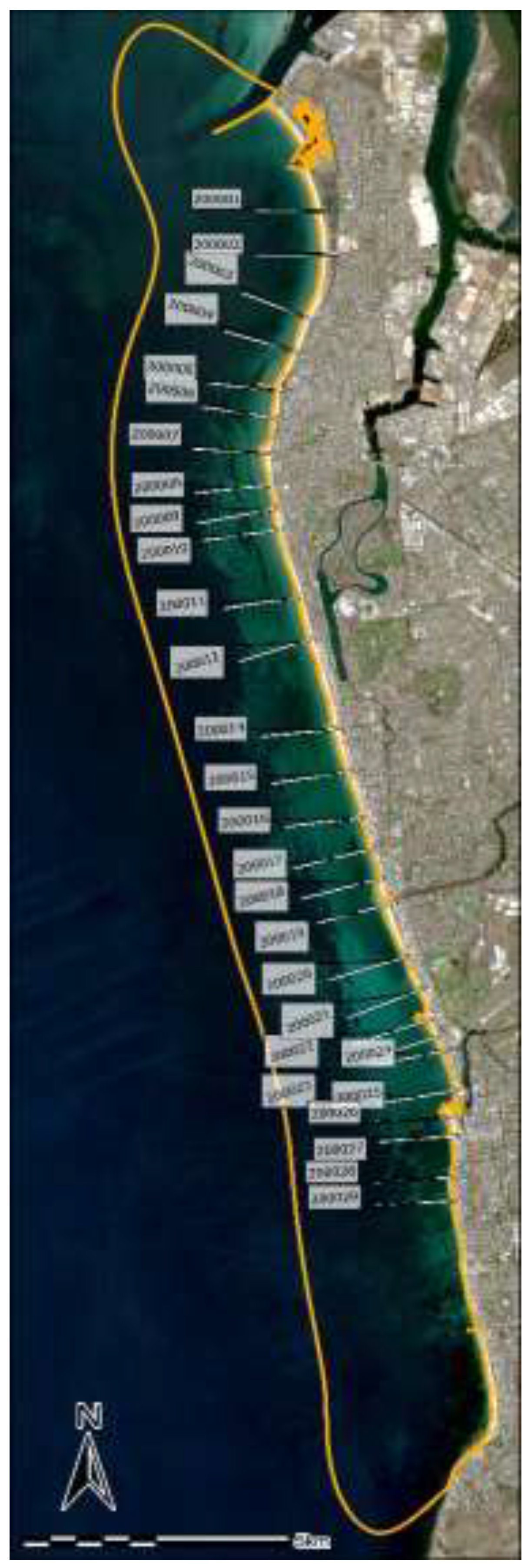
Figure 3.
The frequency distribution of in situ depth data resampled to the pixel size of PlanetScope SuperDove cells (3m) within the sub-site. The distribution is identified as bimodal. Some transparency has been applied to the calibration symbology so an overlap between the two classes may be observed.
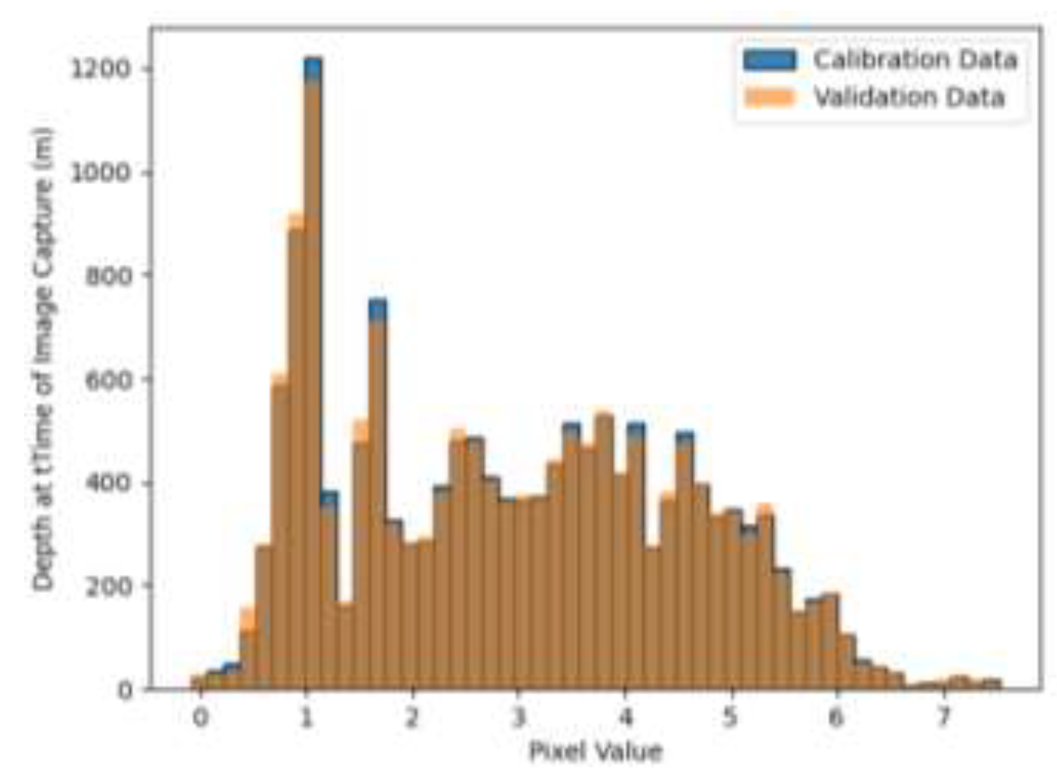
Figure 4.
An overview of technical methods followed to generate and assess the quality of SDB datasets. .
Figure 4.
An overview of technical methods followed to generate and assess the quality of SDB datasets. .
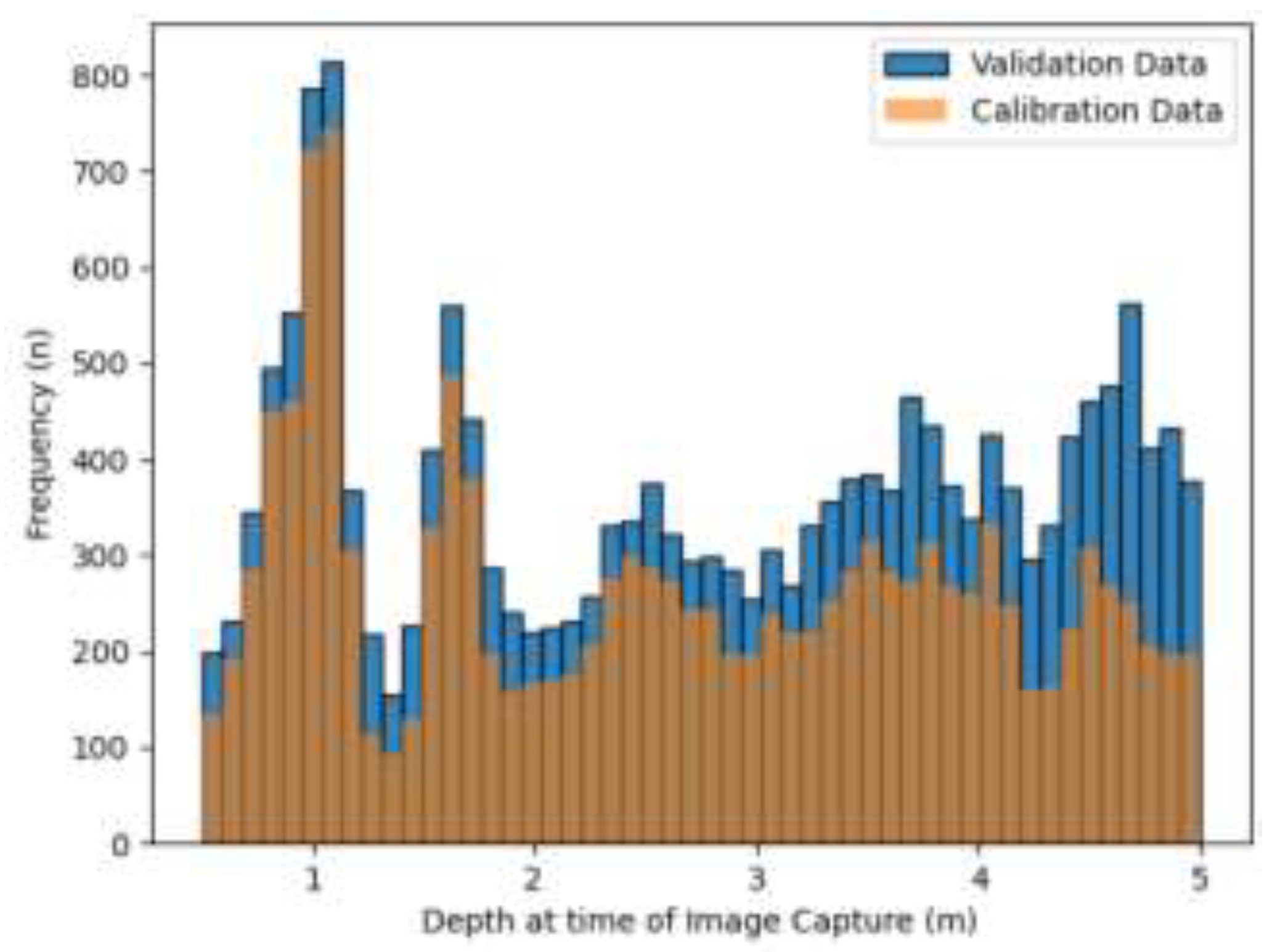
Figure 5.
The frequency distribution of in situ depth data resampled to the pixel size of PlanetScope SuperDove cells (3m) within the study site.
Figure 5.
The frequency distribution of in situ depth data resampled to the pixel size of PlanetScope SuperDove cells (3m) within the study site.
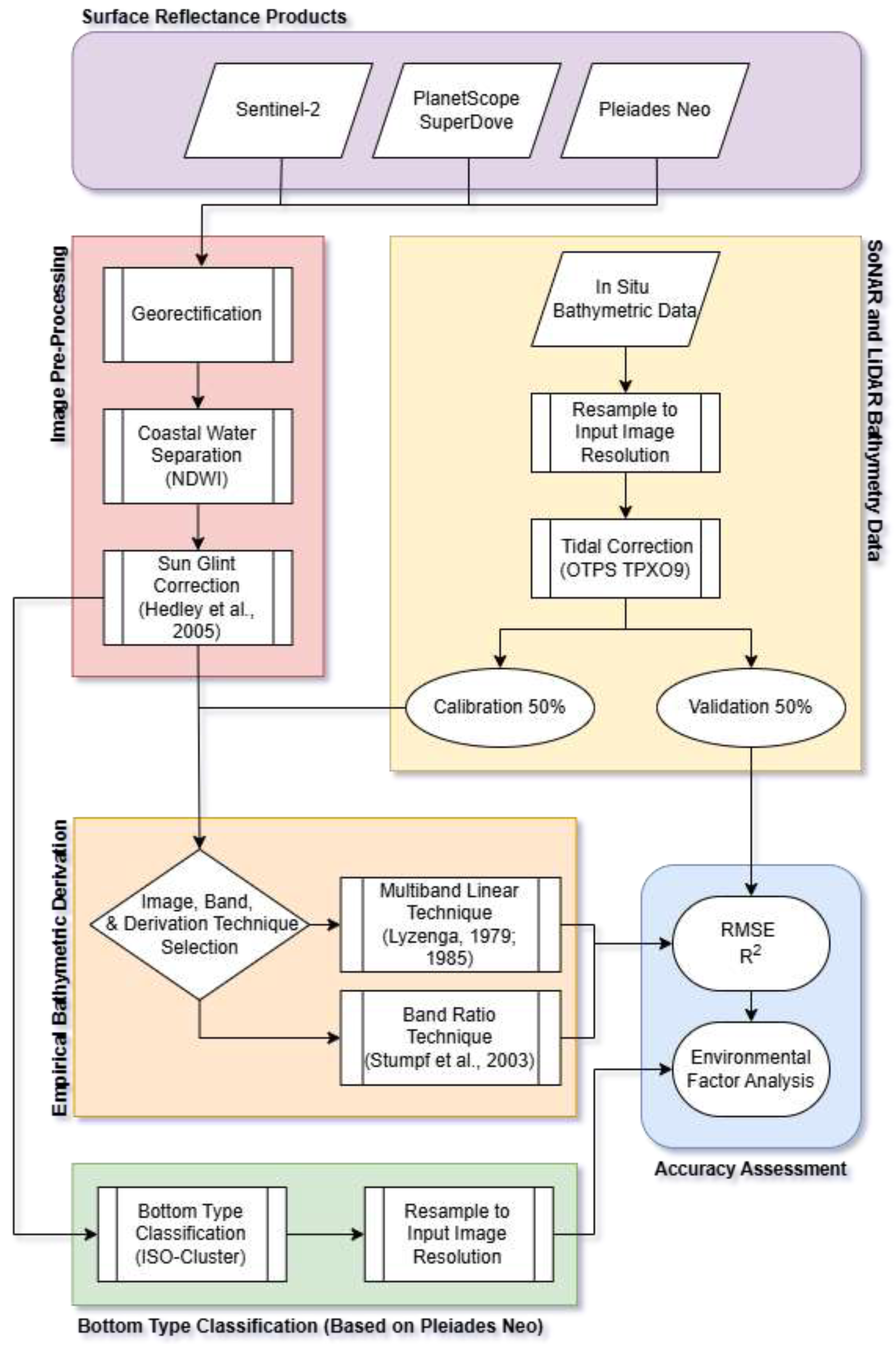
Figure 6.
Before (A) and after (B) the sunglint correction is applied over Pleiades Neo RGB satellite imagery. The imagery is stretched using a minimum/maximum stretch over the displayed extent.
Figure 6.
Before (A) and after (B) the sunglint correction is applied over Pleiades Neo RGB satellite imagery. The imagery is stretched using a minimum/maximum stretch over the displayed extent.
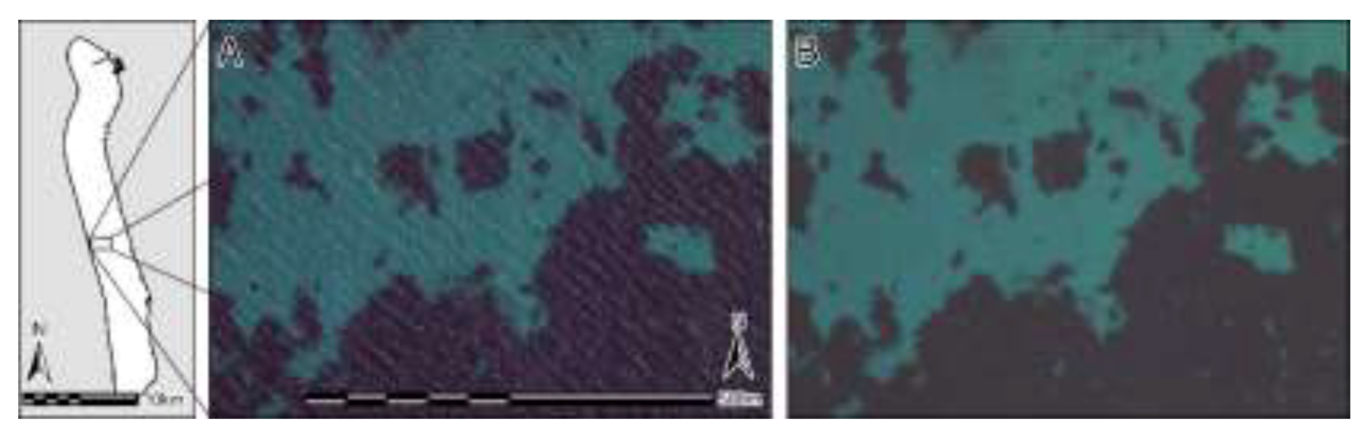
Figure 7.
Depiction of the impact of sunglint correction in shallow water where NIR bottom reflectance is present. Spectral profiles are extracted from the Pleiades Neo multi-spectral image along profile 200015. Spectral profiles have been extracted before sunglint correction was applied, and after sunglint correction was applied. Associated Pleiades Neo RGB satellite imagery is stretched using a minimum/maximum stretch over the marine inundated areas in the displayed extent.
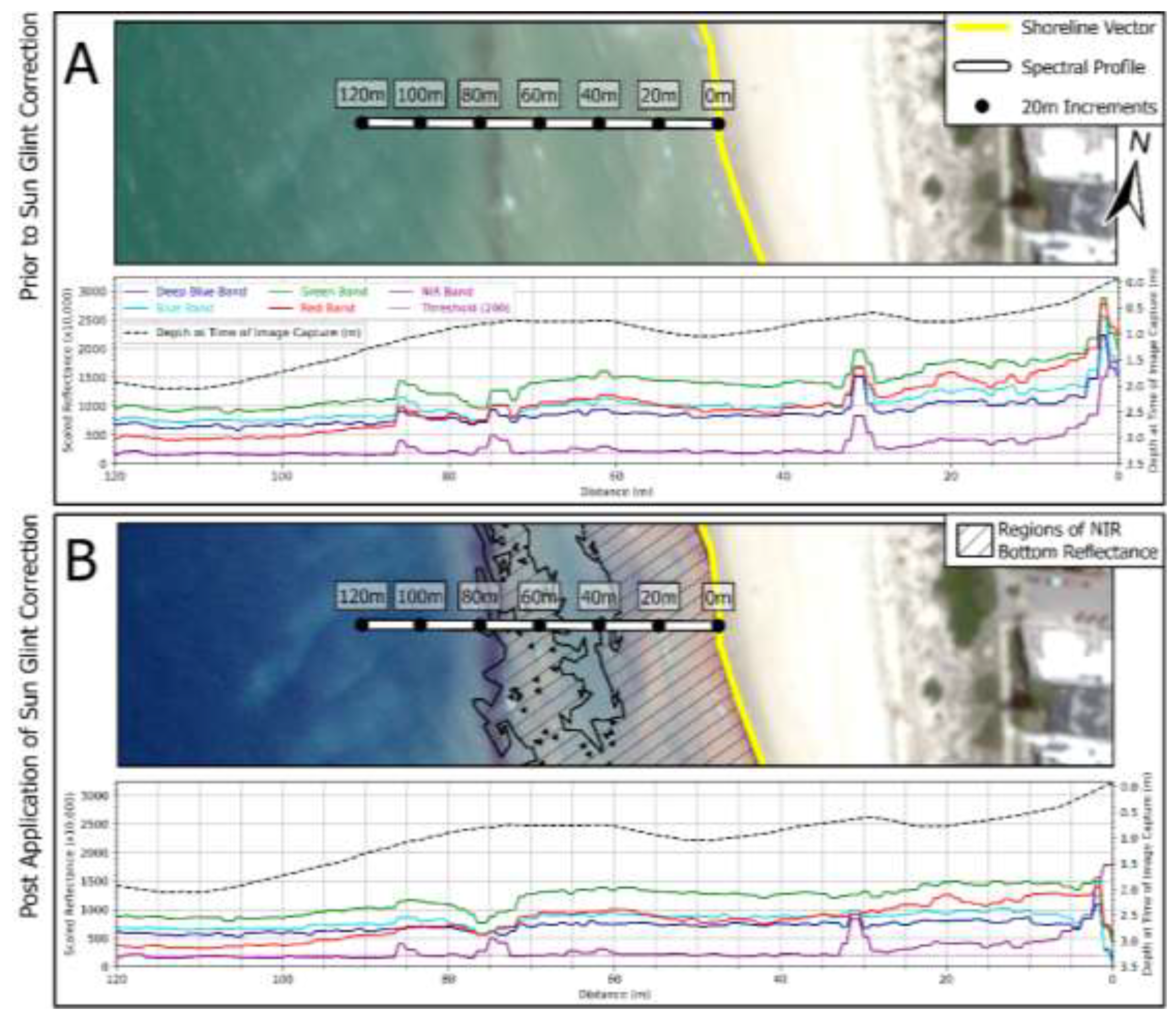
Figure 8.
A depiction of the bathymetric LiDAR surface generated seaward of the shoreline at the time of multi-spectral image capture and its comparison with available SoNAR data within the sub-site (Profile 200004) captured on the same day. All elevations given are in relation to Australian Height Datum (AHD) (m). Pleiades Neo red-green-blue (RGB) imagery underlies the bathymetric raster.
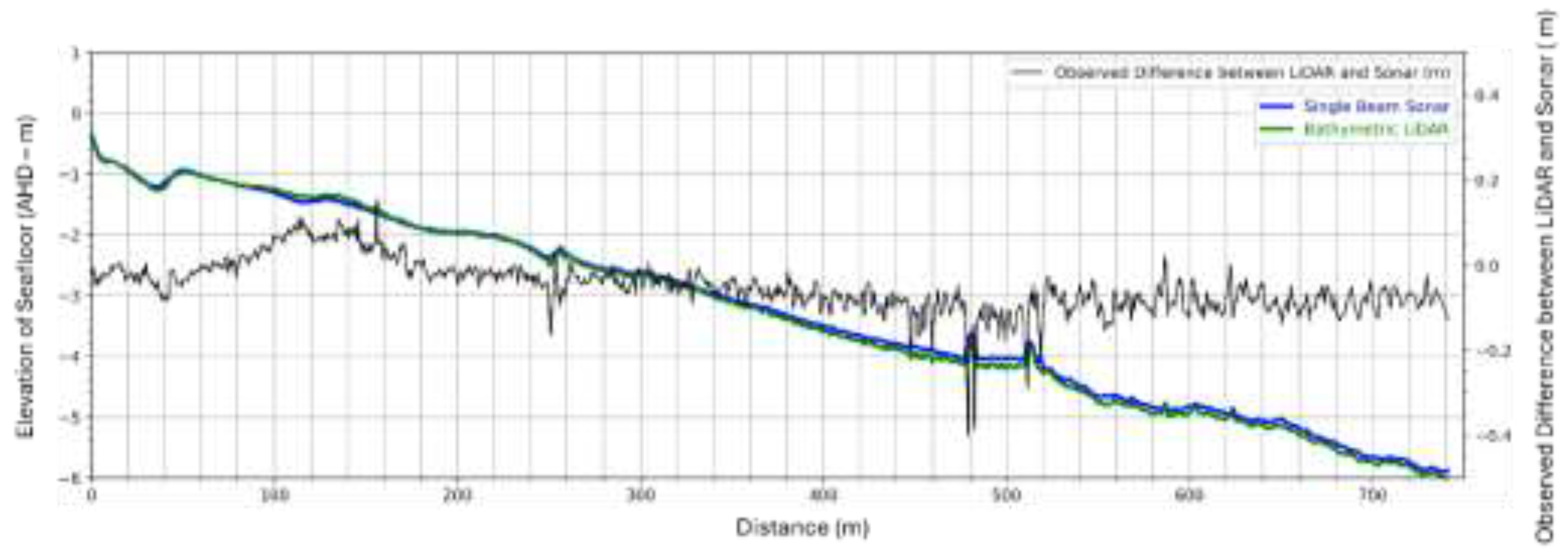
Figure 9.
Comparison between TPXO 9 global tide model and the observed sea-surface height along the length of the study site.
Figure 9.
Comparison between TPXO 9 global tide model and the observed sea-surface height along the length of the study site.
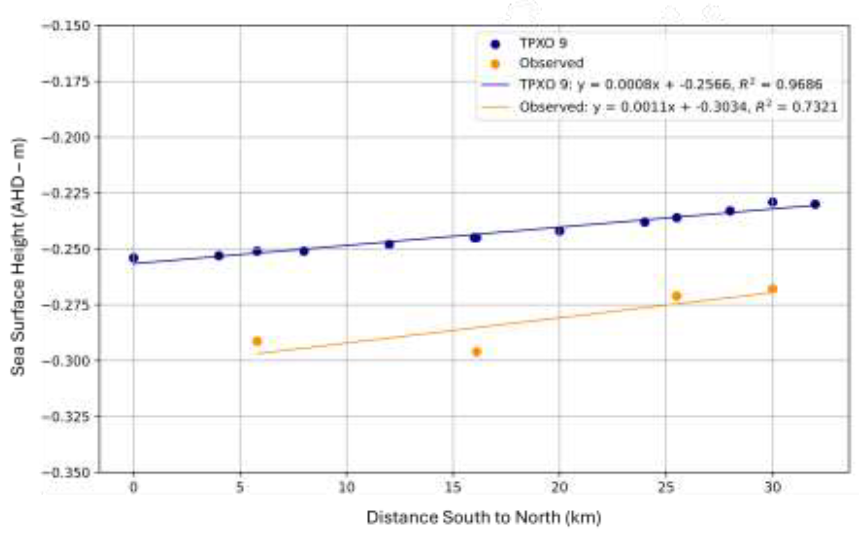
Figure 10.
Boxplots depicting RMSE values for different combinations of satellite imagery and derivation techniques. mean (x̄), third quartile (Q3), and maximum.
Figure 10.
Boxplots depicting RMSE values for different combinations of satellite imagery and derivation techniques. mean (x̄), third quartile (Q3), and maximum.
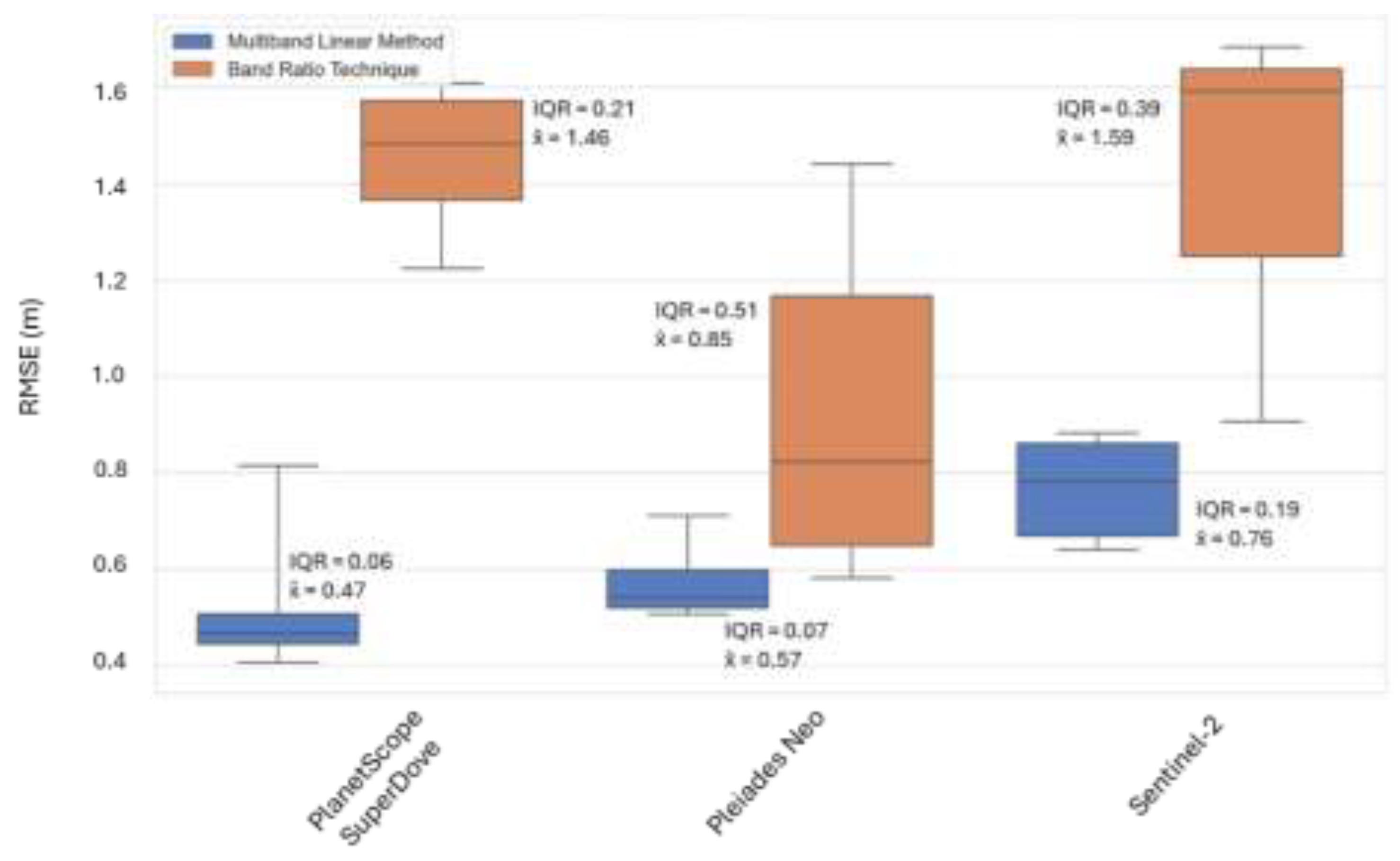
Figure 11.
Depth at time of image capture inferred from the optimised derivation (multiband linear technique on PlanetScope SuperDove using, G-alt, G and Y Bands) plotted against validation data present within the sub-site.
Figure 11.
Depth at time of image capture inferred from the optimised derivation (multiband linear technique on PlanetScope SuperDove using, G-alt, G and Y Bands) plotted against validation data present within the sub-site.
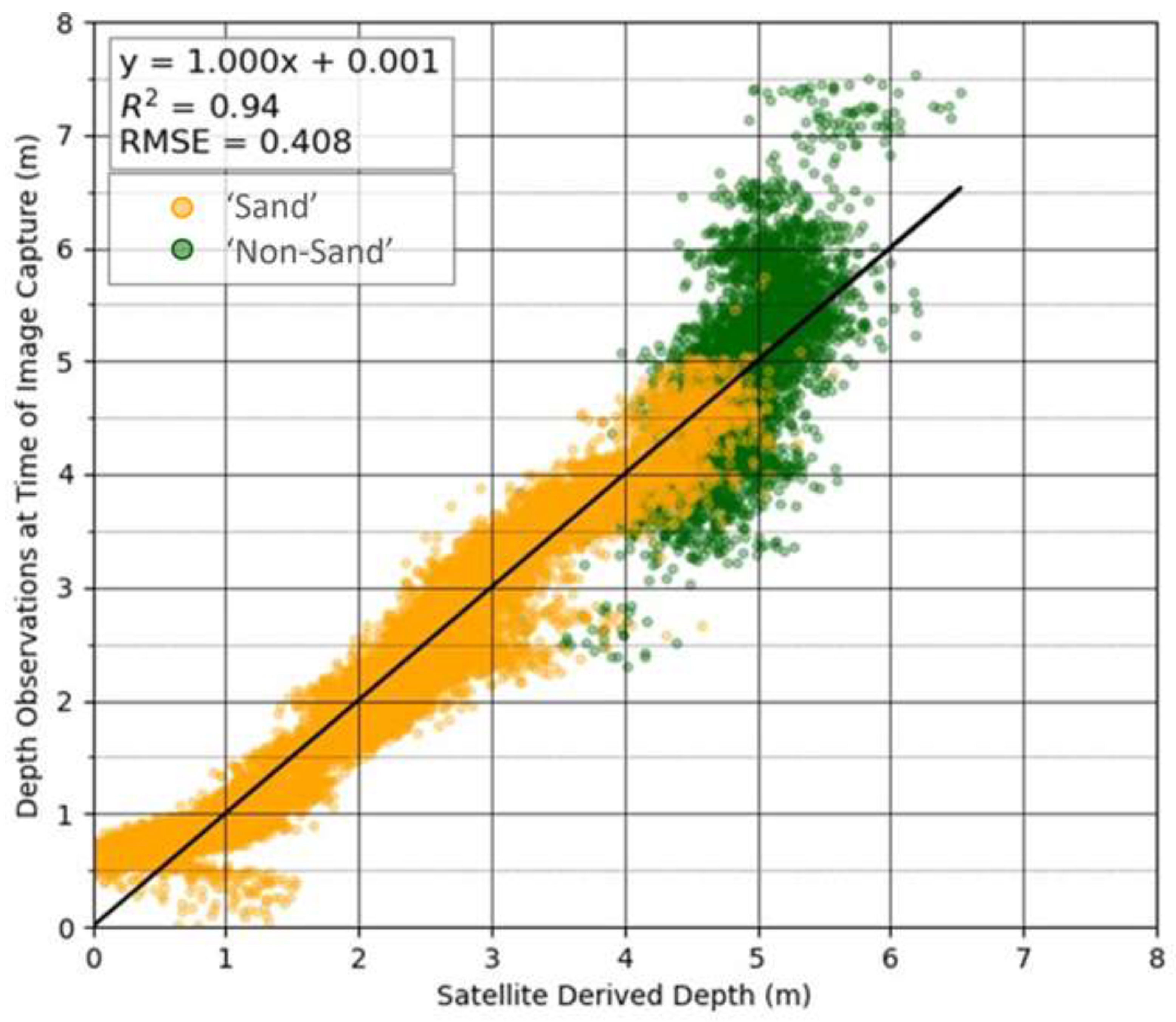
Figure 12.
A depiction of the optimal SDB surface within the sub-site which represents depth at the time of image capture and a comparison with available tidally corrected validation data along profile 200004. Pleiades Neo RGB imagery underlies the bathymetric raster.
Figure 12.
A depiction of the optimal SDB surface within the sub-site which represents depth at the time of image capture and a comparison with available tidally corrected validation data along profile 200004. Pleiades Neo RGB imagery underlies the bathymetric raster.
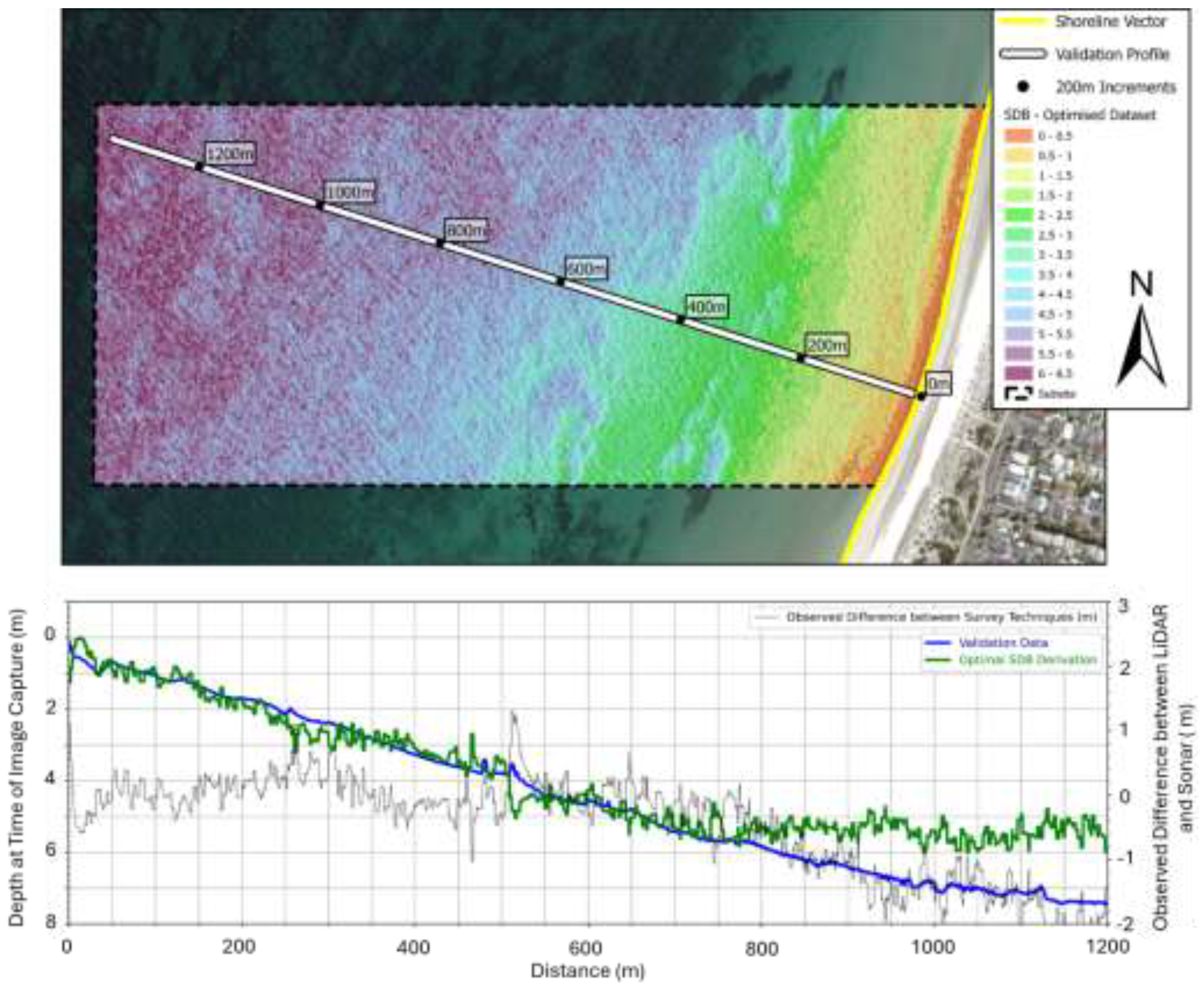
Figure 13.
A 3D representation of the model explaining the greatest variance, incorporating both spectral suitability and pixel size (m). RMSE (m) = 0.1748 + 0.1934 * (Spectral Suitability) + 0.0268 * (Pixel Size (m)).
Figure 13.
A 3D representation of the model explaining the greatest variance, incorporating both spectral suitability and pixel size (m). RMSE (m) = 0.1748 + 0.1934 * (Spectral Suitability) + 0.0268 * (Pixel Size (m)).
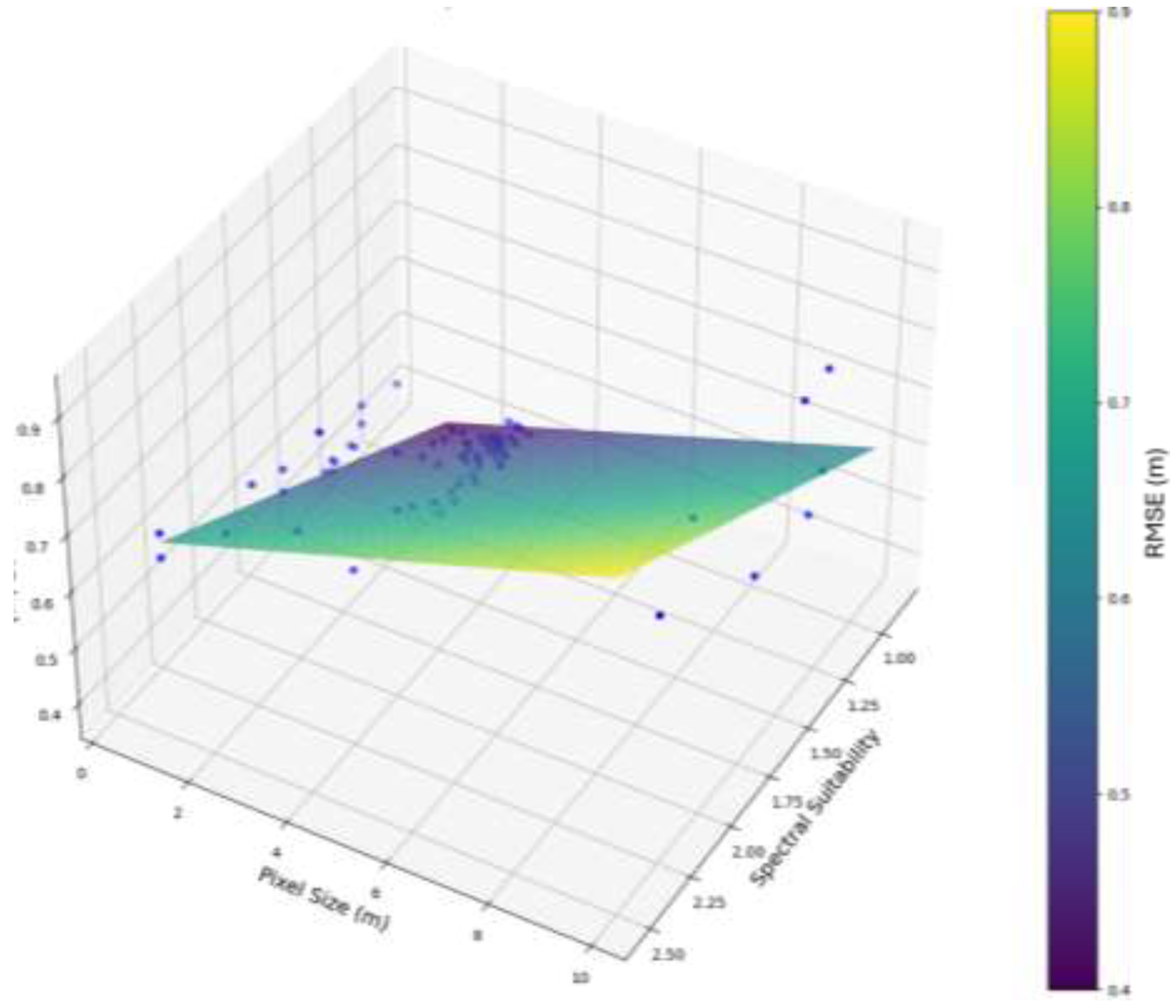
Figure 14.
Validation of the optimised dataset across the entire study site using calibration data obtained within the sub-site. The dashed box encapsulates 9.6% of observations where the SDB surface markedly underestimated depth (2-2.75m), these observations are associated with a discrete, higher-albedo sandy substrate in the south of the site. .
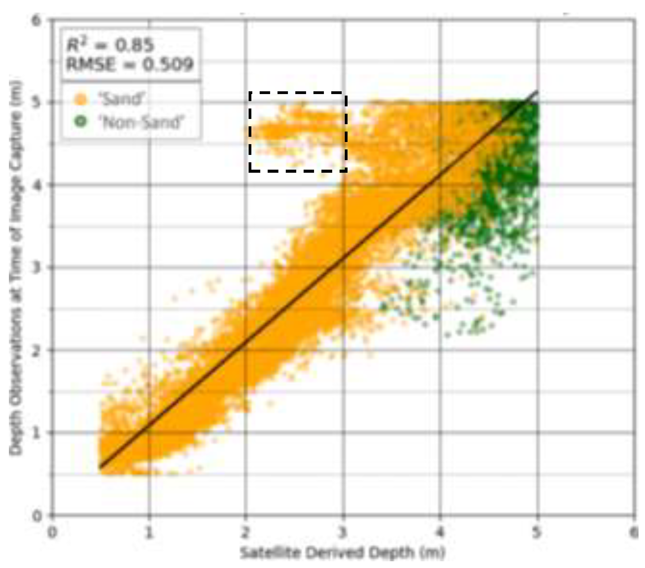
Figure 15.
An illustration and quality assessment of the optimised derivation method applied across the entire study site. The first pane depicts the optimised surface restricted between 0.5m and 5m depth at time of image capture.The second pane presents an enlarged view of the three profiles (200001, 200014, 200027) and presents raw imagery, bottom type classification, and the optimised SDB dataset. The third pane details the cross-shore bathymetry from both the satellite derivation and the true depth across the three profiles, along with the difference between the two survey methods on the secondary axis. The landward extent of ‘non-sand’ pixels is shown with the magenta dashed line.Some gaps exist in the SDB estimation because of depth being restricted between 0.5-5m.
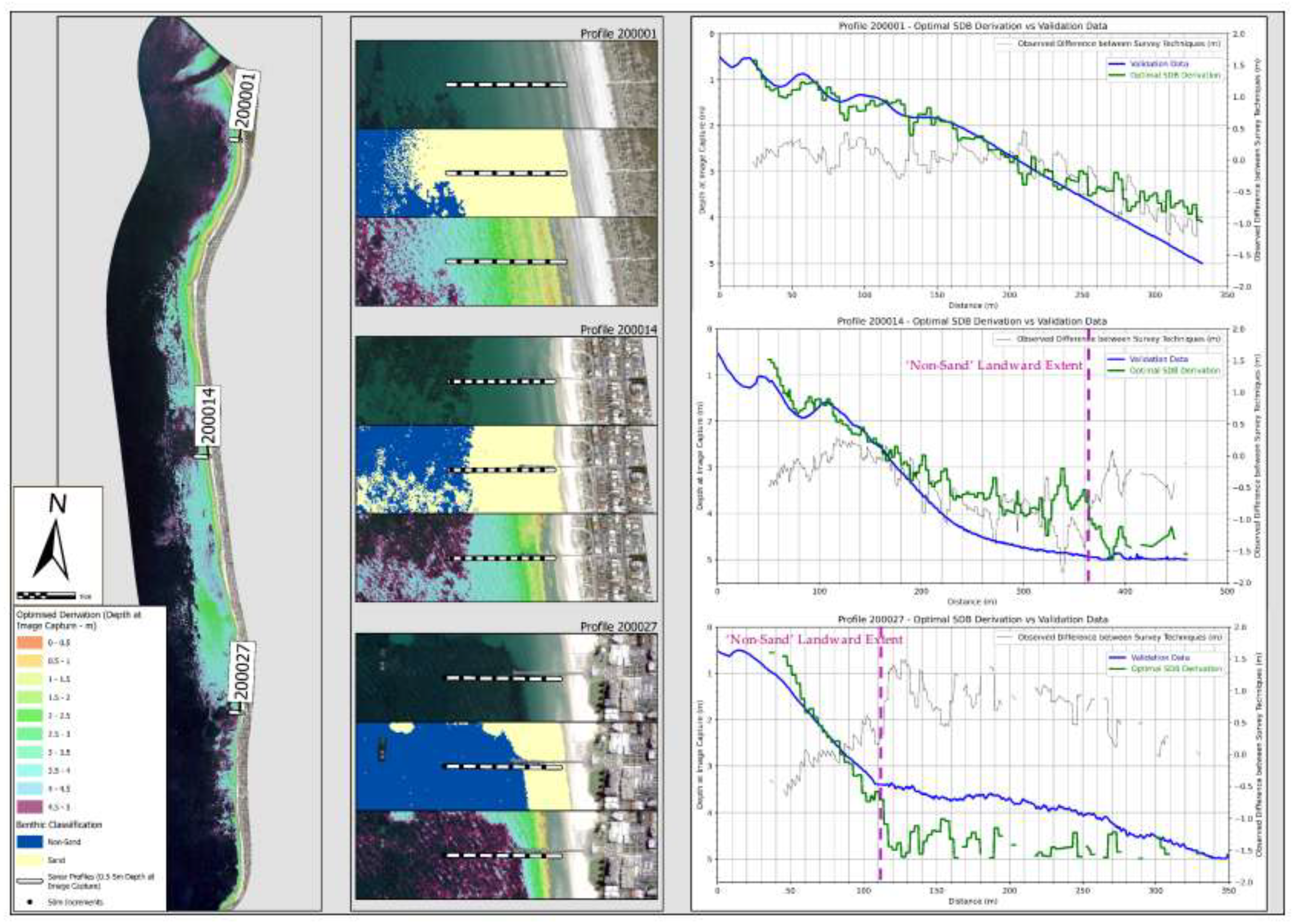
Figure 16.
A depiction of the impact of environmental factors (depth and bottom type) upon dataset quality (mean residual error - m). The figure shows mean residual errors (m) recorded in 1m depth classes and grouped by their bottom type.
Figure 16.
A depiction of the impact of environmental factors (depth and bottom type) upon dataset quality (mean residual error - m). The figure shows mean residual errors (m) recorded in 1m depth classes and grouped by their bottom type.
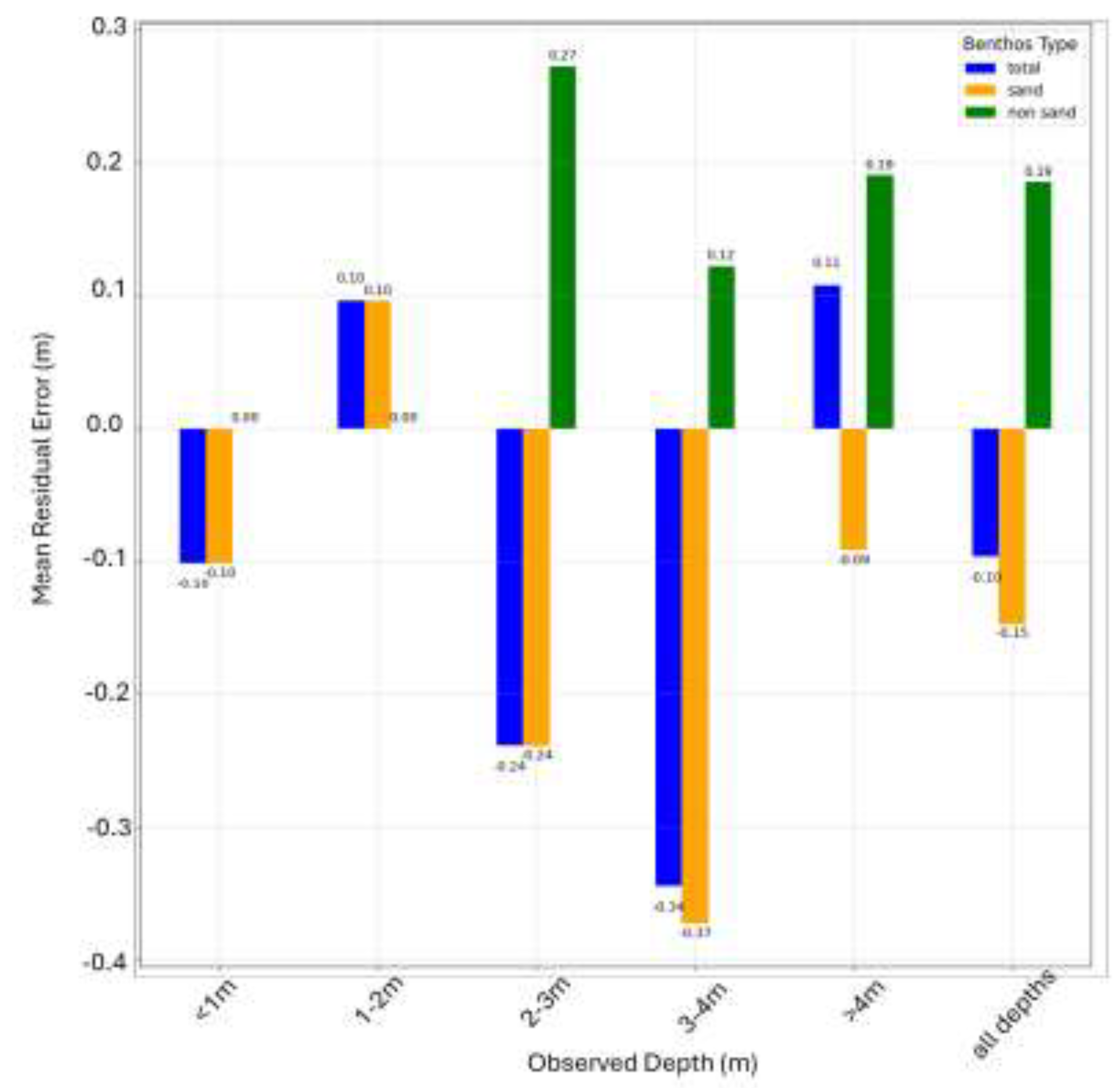
Figure 17.
The frequency distribution of in situ depth data classified by whether the pixel is affected or unaffected by NIR bottom reflectance at time of image capture. Where depth is less than 0.88m most pixel observations were affected by NIR bottom reflectance.
Figure 17.
The frequency distribution of in situ depth data classified by whether the pixel is affected or unaffected by NIR bottom reflectance at time of image capture. Where depth is less than 0.88m most pixel observations were affected by NIR bottom reflectance.
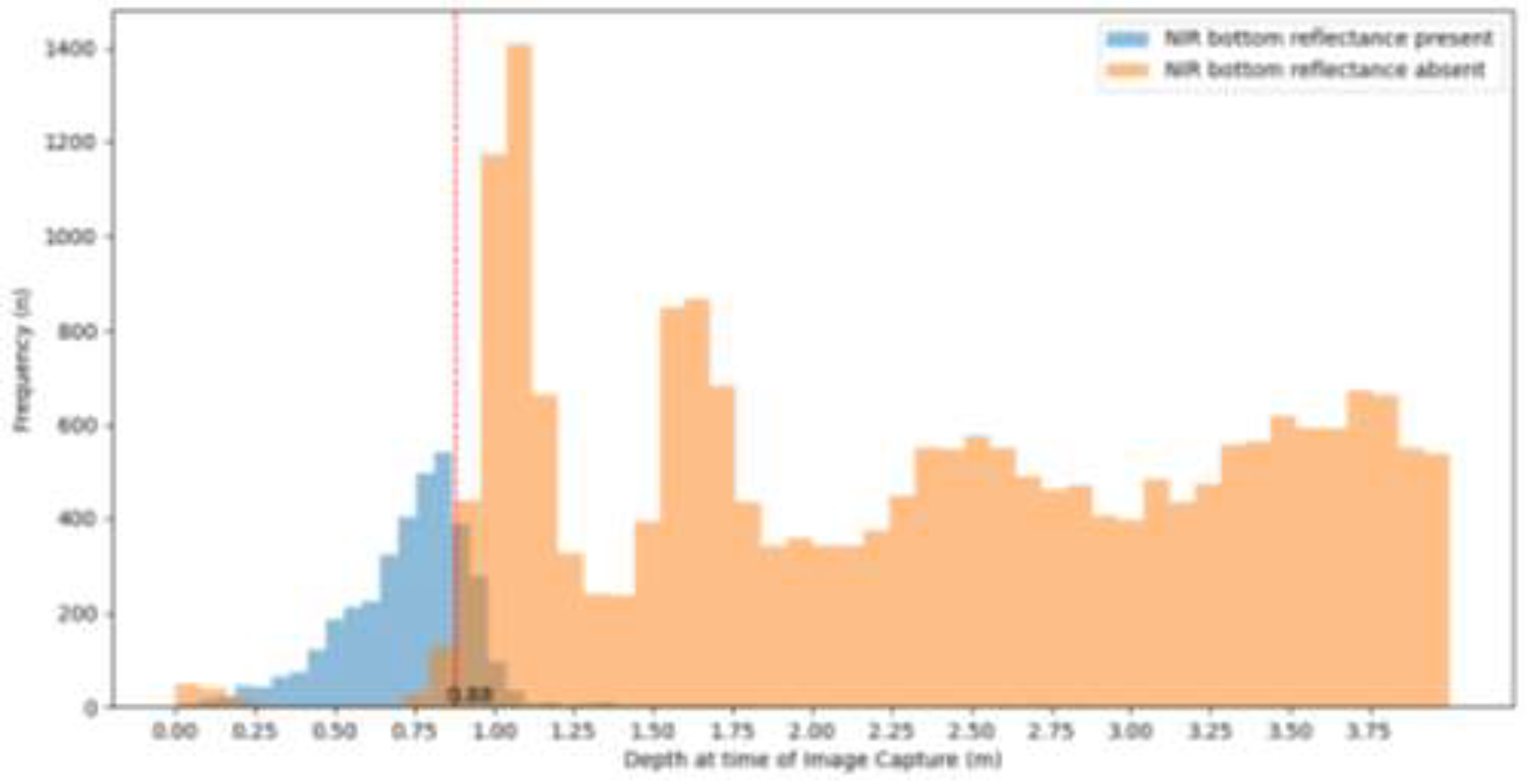

Table 1.
A multi-spectral instrument overview for each of the utilised images within the visible range. Band IDs have been standardised to with a master band ID.
Table 1.
A multi-spectral instrument overview for each of the utilised images within the visible range. Band IDs have been standardised to with a master band ID.
| Sentinel-2 (10m) | PlanetScope SuperDove (3m) | Pléiades Neo (1.2m) | |||||
|---|---|---|---|---|---|---|---|
| Master Band ID | Band Name | Band ID | Wavelength (nm) | Band ID | Wavelength (nm) | Band ID | Wavelength (nm) |
| 1 | Deep Blue | 1 | Discarded due to 60m resolution | 1 | 431-452 | 1 | 400-450 |
| 2 | Blue | 2 | 459-525 | 2 | 465-515 | 2 | 450-520 |
| 3 | Green (alt) | - | - | 3 | 513-549 | - | - |
| 4 | Green | 3 | 541-577 | 4 | 547-583 | 3 | 530-590 |
| 5 | Yellow | - | - | 5 | 600-620 | - | - |
| 6 | Red | 4 | 649-680 | 6 | 650-680 | 4 | 620-690 |
Table 2.
Metadata of the satellite imagery used in the study
| Satellite | Product ID | Acquisition Date | Acquisition Time (UTC +10:30) |
|---|---|---|---|
| Sentinel-2 | S2A_MSIL2A_20240121T003701_N0510_R059_T54HTG_20240121T030545 | 21st Jan 2024 | 11:07:01 |
| PlanetScope SuperDove | 20240121_004724_68_2478_3B_AnalyticMS_8b | 21st Jan 2024 | 11:17:24 |
| Pléiades Neo | PNEO3_202401210048521_MS-FS_ORT | 21st Jan 2024 | 11:18:52 |
Table 3.
Published georectification residual error.
| Satellite Image | Control Points (n) | Total XY RMSE (m) | Total XY RMSE (pixel) |
|---|---|---|---|
| Pleiades Neo | 10 | 0.48 | 0.4 |
| PlanetScope SuperDove | 87 | 2.77 | 0.92 |
| Sentinel-2 | 70 | 5.4 | 0.54 |
Table 4.
Logging parameters of local tide gauges.
| Tide Gauge ID | Type | Events per second (Hz) | Duration (min) | Interval (min) |
|---|---|---|---|---|
| 1, 2, 3 | RBR virtuso3 | 16 | 1 | 5 |
| 4 | Data Logger Mindata / Hadar 4500 / 555 | 1 | 1 | 5 |
Table 5.
Ranked candidate MLR models used to explain the impact of predictor variables spectral suitability and pixel size (m) upon the response variable RMSE (m).
Table 5.
Ranked candidate MLR models used to explain the impact of predictor variables spectral suitability and pixel size (m) upon the response variable RMSE (m).
| Derivation Technique | Observations (n) | Predictor Variables | Model Equation | R2 | AIC | ER |
|---|---|---|---|---|---|---|
| Multiband Linear | 85 | Spectral Suitability, Pixel Size (m) | RMSE (m) = 0.1748 + 0.1934 * (Spectral Suitability) + 0.0268 * (Pixel Size (m)) | 0.78 | -262.6736 | 1 |
| Spectral Suitability | RMSE (m) = 0.2563 + 0.1976 * (Spectral Suitability) | 0.49 | -193.5218 | 7.26×10¹⁵ | ||
| Pixel Size (m) | RMSE (m) = 0.4334 + 0.0277 * (Pixel Size (m)) | 0.31 | -168.5168 | 3.38×10²⁰ | ||
| Band Ratio | 24 | Spectral Suitability, Pixel Size (m) | RMSE (m) = 1.6484 + -0.2993 * (Spectral Suitability) + 0.0296 * (Pixel Size (m)) | 0.14 | 16.3757 | 1.312 |
| Spectral Suitability | RMSE (m) = 1.8404 + -0.3624 * (Spectral Suitability) | 0.08 | 15.8323 | 1 | ||
| Pixel Size (m) | RMSE (m) = 1.1969 + 0.0359 * (Pixel Size (m)) | 0.08 | 15.8452 | 1.007 |
Disclaimer/Publisher’s Note: The statements, opinions and data contained in all publications are solely those of the individual author(s) and contributor(s) and not of MDPI and/or the editor(s). MDPI and/or the editor(s) disclaim responsibility for any injury to people or property resulting from any ideas, methods, instructions or products referred to in the content. |
© 2025 by the authors. Licensee MDPI, Basel, Switzerland. This article is an open access article distributed under the terms and conditions of the Creative Commons Attribution (CC BY) license (http://creativecommons.org/licenses/by/4.0/).
Copyright: This open access article is published under a Creative Commons CC BY 4.0 license, which permit the free download, distribution, and reuse, provided that the author and preprint are cited in any reuse.


