
Submitted:
23 January 2026
Posted:
23 January 2026
You are already at the latest version
Abstract
Critical slowing down and topological freezing in lattice gauge theory can be aggravated by thegauge-redundant link representation, which obscures simpler geometric structure available in al-ternative variables. We introduce Flux-Space Flow Matching (FFM), a generative samplingframework for 2D compact U(1) theory that operates directly on gauge-invariant flux (plaquette-angle) variables. By formulating the dynamics in flux space, the Wilson action is locally factorized,allowing us to train a continuous-time Neural ODE to approximate the equilibrium distributionwithout suffering from the stiff curvature typical of the coupled link formulation. We impose theglobal topological sector constraint via a deterministic “Relax-and-Project” mechanism and applyan independent Metropolis–Hastings accept/reject step as a bias-control procedure. Validated onL∈{48,64}lattices, FFMachievesacceptanceratesof50–70% atL= 48 andreducestheintegratedautocorrelation time of the topological charge by over 500×compared to Hybrid Monte Carlo atβ = 6.0 (on our run lengths). We validate model fidelity against thermodynamic observables, Wilsonloops, and Creutz ratios, finding agreement with the expected non-perturbative confinement scalingwithinthetestedregime. Furthermore, wedemonstratethatSpatialβ-Conditioningenableszero-shot approximation of inhomogeneous thermodynamics, spontaneously nucleating vortex–antivortexpairs in response to spatially varying coupling profiles. These results suggest that identifying theappropriate geometric degrees of freedom can be a more effective path to scalable neural samplingthan architectural complexity alone.
Keywords:
Lattice Gauge Theory
; machine learning
; AI4Science
1. Introduction
Lattice Gauge Theory (LGT) provides the non-perturbative framework for studying gauge fields. The standard method for numerical estimation is Hybrid Monte Carlo (HMC). However, as the lattice spacing decreases towards the continuum limit, HMC algorithms exhibit critical slowing down and topological freezing, which increase the autocorrelation time of observables.
Generative neural sampling methods aim to mitigate this by producing independent configurations [1,2,3]. Normalizing Flows, specifically Gauge Equivariant Flows [4], have demonstrated the ability to sample without autocorrelation by building symmetries directly into the network architecture. Following proof-of-principle studies [4,5], recent work has focused on scalable architectures for high-dimensional manifolds [2,6]. However, the standard approach relies on equivariant coupling layers [7]. While these architectures rigorously preserve symmetry, they often incur prohibitive costs due to determinant computations or restricted expressivity.
In this work, we are motivated by classic duality and Villain-type analyses of the 1980s [8,9], which make the topological excitation content of compact Abelian models explicit and highlight the utility of flux/defect-based representations. Historically, such duality transformations have allowed physicists to map a system with complex constraints or strong couplings into a dual space where the degrees of freedom decouple or become weakly interacting, offering a significant computational advantage. We leverage this principle to circumvent the limitations of direct link-based sampling.
We propose Flux-Space Flow Matching (FFM), a framework for Compact LGT that integrates three specific components.
First, we transform the problem usage from link variables to gauge-invariant dual flux variables. In this representation, the local Bianchi identity becomes vacuous, yet we explicitly acknowledge that the global constraint imposed by the toroidal geometry remains.
Second, to address critical slowing down, we implement Spatial -Conditioning, replacing global scalar conditioning with a local field.
Third, we build on the Flow Matching framework [10], which regresses the neural vector field onto optimal transport paths, offering superior stability over likelihood-based training. This formulation relates to the Probability Flow ODE of Score-Based Models [11], identifying the generative process as a deterministic flow [12].
We demonstrate that FFM enables scalable sampling on lattices with stable Metropolis correction, and—by validating against thermodynamic, confinement, and topology-sensitive observables—show that it achieves high-fidelity ensembles, bridging geometric deep learning with lattice-sampling methodology grounded in statistical mechanics.
2. Background
2.1. Link to Flux Transformation
Transformation. Standard LGT is formulated in terms of link variables defined on oriented edges of a periodic square lattice (a 2-torus). Here denotes a lattice site, are direction indices, and is the unit vector in direction . The Wilson action reads
This link formulation induces a dense interaction graph: each link participates in two adjacent plaquettes, producing strong local couplings that lead to a stiff energy landscape and critical slowing down.
Figure 1.
Link to Flux Transformation. Visualization of the mapping from gauge-redundant link variables (edges) to gauge-invariant flux variables (plaquettes).
Figure 1.
Link to Flux Transformation. Visualization of the mapping from gauge-redundant link variables (edges) to gauge-invariant flux variables (plaquettes).
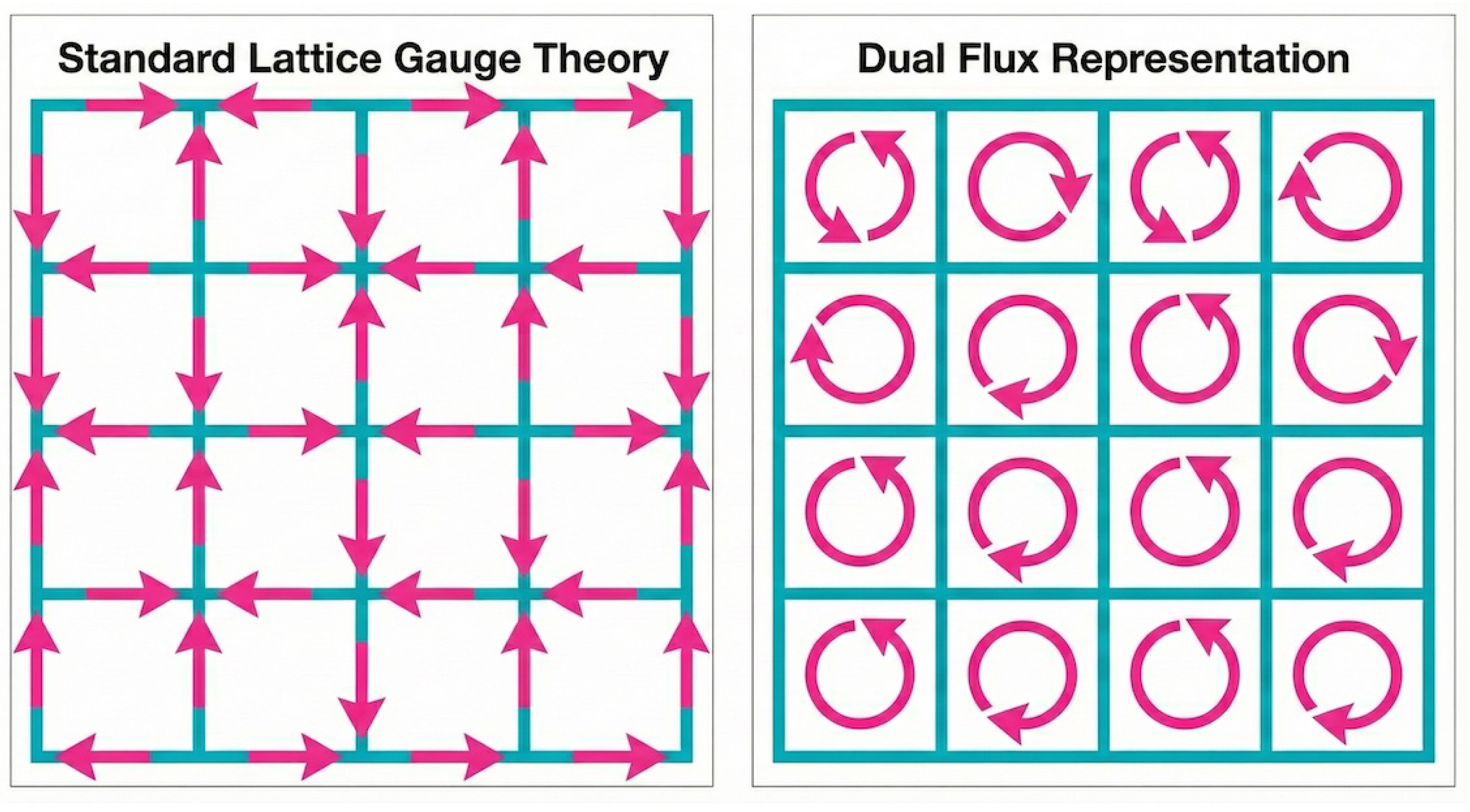
To mitigate this, we change variables from links to plaquette degrees of freedom. Let denote an oriented plaquette and define the Wilson plaquette variable
Throughout this work, we use the term flux to refer to the plaquette angle (equivalently, to the plaquette phase ). In this basis the action becomes
Let denote the lattice volume; in on an torus, V equals the total number of plaquettes (and also the number of sites). Ignoring global constraints and measure effects, the local statistical weight is well-approximated by the factorized form
which yields a locally factorized optimization and sampling landscape compared to the coupled link formulation. Throughout, our goal is computational efficacy and empirical correctness of lattice observables, not a one-to-one reproduction of a specific analytic dual construction; in particular, the link-to-plaquette map is many-to-one, and the induced plaquette measure includes gauge redundancy and (on the torus) global degrees of freedom.
Absence of Local Constraints. A potential concern is whether an arbitrary plaquette field corresponds to a valid underlying link configuration. In two dimensions, the usual local Bianchi identity is vacuous because there are no 3-cells (), so no local geometric consistency constraint couples neighboring plaquettes. Moreover, as detailed in Appendix A, on any simply connected patch with boundary, implies local realizability: every plaquette configuration on can be reproduced by a (gauge-fixed) assignment of links. Thus, in there are no local constraints that re-introduce dynamical coupling beyond the factorized plaquette action.
Global Sector Constraint on the Torus. Consequently, the remaining stiffness is global and topological on , manifesting as the quantization of the total flux (topological charge)
with the precise lifting/branch structure discussed in Appendix A. We enforce this global sector constraint via a manifold-style projector (“Relax-and-Project”) and use an independent Metropolis–Hastings accept/reject step as a bias-control mechanism (Section 3.3).
2.2. Spatial -Conditioning
A key architectural choice in our conditional generator is to avoid injecting a global conditioning vector into every layer and instead present the inverse coupling as a spatial channel. Concretely, we lift the scalar to a field (constant in the homogeneous case, but representable as spatially varying in general) and concatenate it with the flux representation at the network input:
This is a reasonable inductive bias for locality and translation-equivariance: is provided in the same tensor format as the physical degrees of freedom, and its influence on the generated configuration is mediated through the same local convolutional computations rather than through per-layer global modulation pathways (e.g., FiLM-style feature-wise affine transforms).
This design is particularly relevant near criticality. Markov-chain methods propagate information through a sequence of updates, so long-range correlations emerge only after many steps and suffer from critical slowing down. In contrast, our model produces an entire configuration in parallel. Although the conditioning enters locally via , the deep hierarchical network has an effective receptive field that can span the lattice (via depth and/or dilation), enabling the synthesis of the long-range correlations required at large correlation length within a single forward pass. This does not eliminate the need for an exactness mechanism when required (e.g., a global accept/reject correction), but it amortizes the construction of correlated configurations across values within one trained model.
3. Generative Architecture: FluxUNet
3.1. Network Architecture (FluxUNet)
To implement the FFM framework, we parameterize the time-dependent velocity field using FluxUNet, a specialized Residual U-Net designed for compact angular variables on a toroidal lattice. Several architectural choices are motivated by the geometry of the lattice and by numerical stability of continuous-time flows:
- Toroidal Topology (). All convolutional layers employ circular padding, enforcing periodic boundary conditions and preventing boundary artifacts.
- Residual Parameterization. We use residual blocks, , which bias the network toward incremental feature updates rather than abrupt re-mappings. This typically stabilizes optimization and reduces spurious high-frequency responses. In our setting, it yields smoother spatial predictions under periodic convolutions and improves numerical robustness.
- Smooth Nonlinearity and Normalization. We use SiLU activations and Group Normalization () instead of ReLU or BatchNorm. SiLU provides a smooth nonlinearity, and GroupNorm avoids dependence on batch statistics, which is beneficial when training vector fields with small or varying batch sizes.
3.2. Training Strategy: Ensemble Distillation
We generate the training corpus using massively parallel persistent local Metropolis chains with a checkerboard update scheme; all hyperparameters (warmup, decorrelation interval, proposal amplitude, and scheduling) are documented in Appendix B. While individual short chains may remain trapped in metastable regions of configuration space, aggregating many chains initialized from random hot starts () yields broad empirical coverage of typical configurations.
We observe an implicit denoising effect consistent with the spectral bias of convolutional networks [13]: the model preferentially captures low-frequency, large-scale structure while being less prone to memorizing high-frequency artifacts present in imperfectly equilibrated training sets. We therefore treat FluxUNet as an ensemble distiller in the empirical sense that its generated configurations exhibit improved agreement of lattice observables with reference results. Any claim of asymptotic correctness is instead attributed to the Metropolis correction described below.
Prior flow-based samplers for LGT often employ stacks of discrete invertible coupling layers [4]. In contrast, we adopt a continuous-time formulation in flux space and train the dynamics with an ODE-style flow matching objective. This provides a smooth transport/denoising learning signal well suited to compact angular variables, and it prioritizes accurate reproduction of lattice observables rather than an explicit analytic dual construction.
3.3. Sector-Projected Metropolis-Corrected Sampling (IMH)
Our simulations impose periodic boundary conditions, so the lattice is topologically a torus and flux configurations decompose into integer total-flux sectors. We therefore include an explicit sector projection step that removes residual non-integer drift in the total flux by shifting only the global mean. We then apply an Independent Metropolis–Hastings (IMH) correction using the model’s estimated proposal density.
Let the target density be . One IMH step proceeds as:
- 1.
- Base distribution. Sample .
- 2.
- Flow proposal (CNF). Integrateusing an adaptive Runge–Kutta solver with tolerance to obtain . In parallel, we track an estimated log proposal density by integrating the instantaneous change-of-variables equation for the flow (divergence of ), using a Hutchinson trace estimator.
- 3.
- Toroidal wrapping. Map the angles to the principal branch
- 4.
-
Nearest-sector projection (global constraint). Compute the total wrapped fluxand project by shifting only the global mean:This step preserves the nearest integer sector label Q and enforces exactly.
- 5.
- IMH acceptance Accept with probability . The acceptance ratio is:
Note on proposal-density estimation and exactness. The sector projection (10) is a deterministic global constraint enforcement that maps unconstrained proposals onto a codimension-one manifold (and is piecewise-defined due to the nearest-sector rounding). As a result, the exact proposal density of the projected samples requires a measure-consistent treatment on the constrained manifold. In addition, the divergence entering is estimated stochastically via Hutchinson, which is unbiased for the trace but does not yield an exact likelihood when exponentiated. For these reasons, the IMH step in (11) should be interpreted as a Metropolis-corrected, bias-limited correction rather than a strictly exact sampler. We provide a quantitative empirical validation of the method’s fidelity and efficiency in the following section.
4. Results: Empirical Validation
We focus our evaluation on Compact LGT on lattices. As detailed in Section 3.2, we utilize a Distilled Ensemble strategy to train on samples () using a single NVIDIA A100 GPU for 20 epochs. All sampling benchmarks employ an adaptive Runge–Kutta integrator (DOPRI5/RK45). We analyze the results from five perspectives.
4.1. Thermodynamic Consistency Checks
We quantify precision by monitoring the Energy Density during training. As shown in Figure 2, the model converges rapidly to the physical manifold. The final ensemble achieves a Mean Absolute Error (MAE) of 0.00095 relative to the theoretical prediction. For a detailed validation against the Von Mises distribution, see Appendix C.
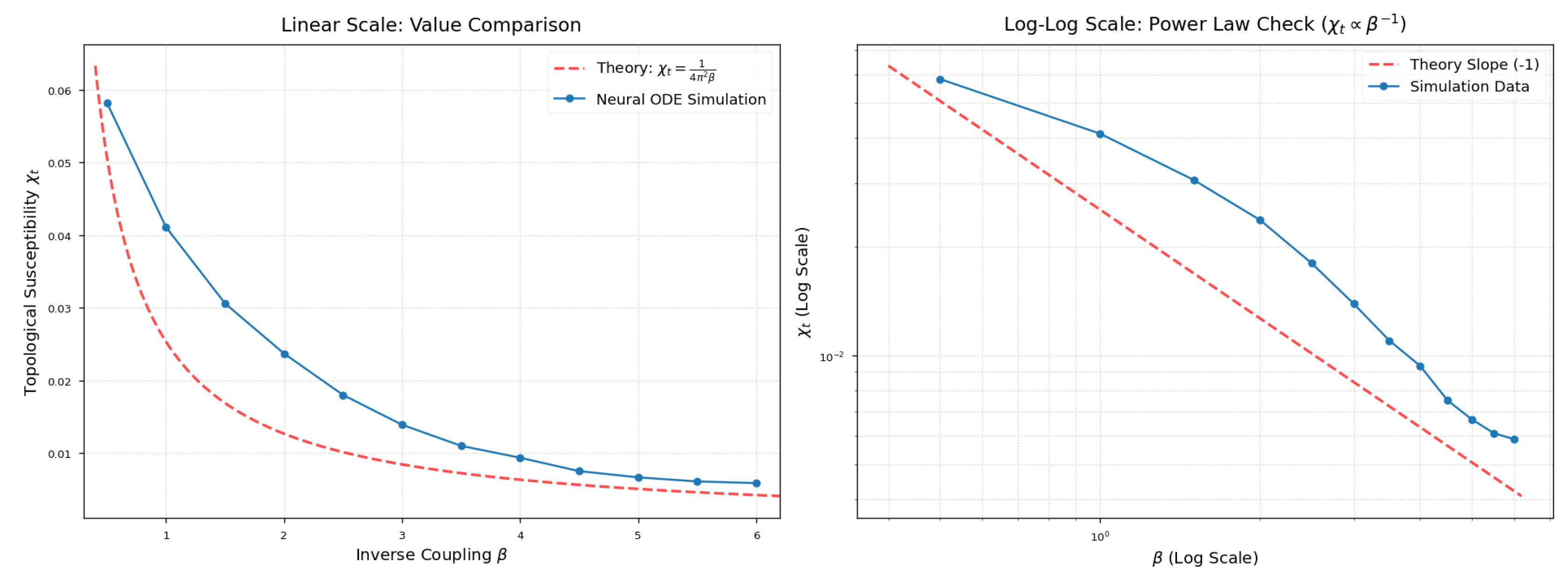
This allows for precise spectroscopy of the topological susceptibility (Figure 3). Notably, our measured susceptibility slightly exceeds the perturbative non-compact limit (). This deviation is physically robust, reflecting the additional contribution from non-perturbative vortex excitations characteristic of the Compact theory, confirming that the generative model captures full non-perturbative dynamics beyond the Gaussian approximation. The deviation at high reflects expected Finite Volume Effects as the correlation length approaches the lattice size L. Finite- reconstructions via phase reweighting and sector-aware reconstruction, reported in Appendix E, further confirm the pipeline’s internal consistency within a statistically controlled analysis window.
4.2. Sampling Efficiency Benchmarks
Performance analysis.Table 1 demonstrates a clear separation between (i) mixing, quantified by , and (ii) absolute wall-clock throughput, quantified by ESS/s. At low coupling (e.g., ), HMC benefits from inexpensive leapfrog updates and achieves substantially higher ESS/s for Q (about higher than FFM in our benchmark). In this regime, our FFM sampler is not wall-clock competitive because the DOPRI5 proposal requires repeated model evaluations and divergence estimation. This is a compute-cost issue rather than a mixing issue, since remains order unity.
At larger , HMC exhibits pronounced topological freezing: at , becomes extremely large with substantial run-to-run variability (), indicating practically non-ergodic behavior on the simulated timescale. In contrast, the conditional FFM sampler maintains across the tested values, yielding a reduction in at .
Crucially, this advantage is amortized across parameter space: the same trained conditional model is used for all , whereas HMC typically requires re-thermalization (and often re-tuning of integrator hyperparameters) at each . Consequently, despite a higher per-step cost, FFM crosses over in absolute wall-clock efficiency for the topological observable at (ESS/s in Table 1), precisely where HMC begins to freeze.
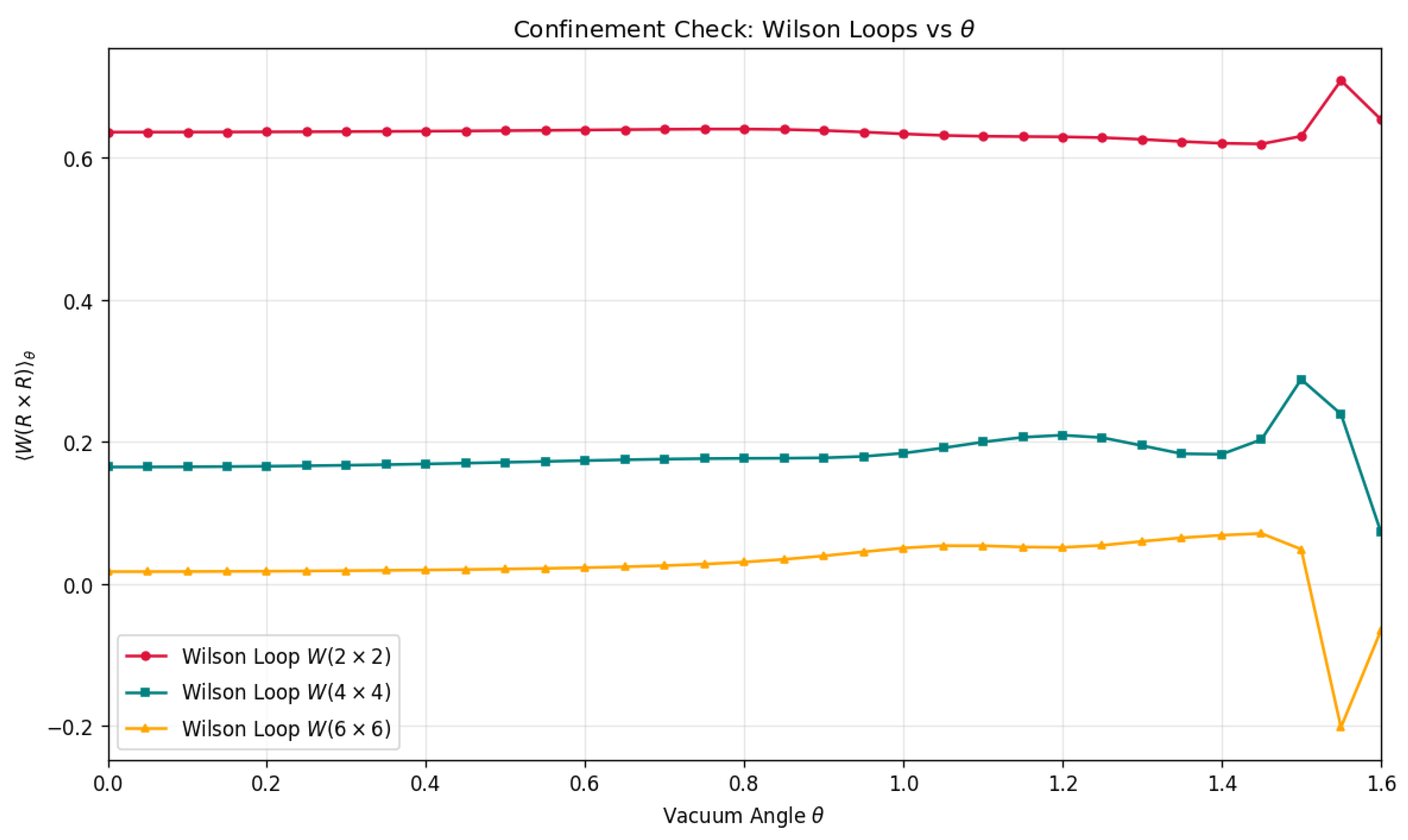
4.3. Confinement Diagnostics: V(R) and Creutz Ratios
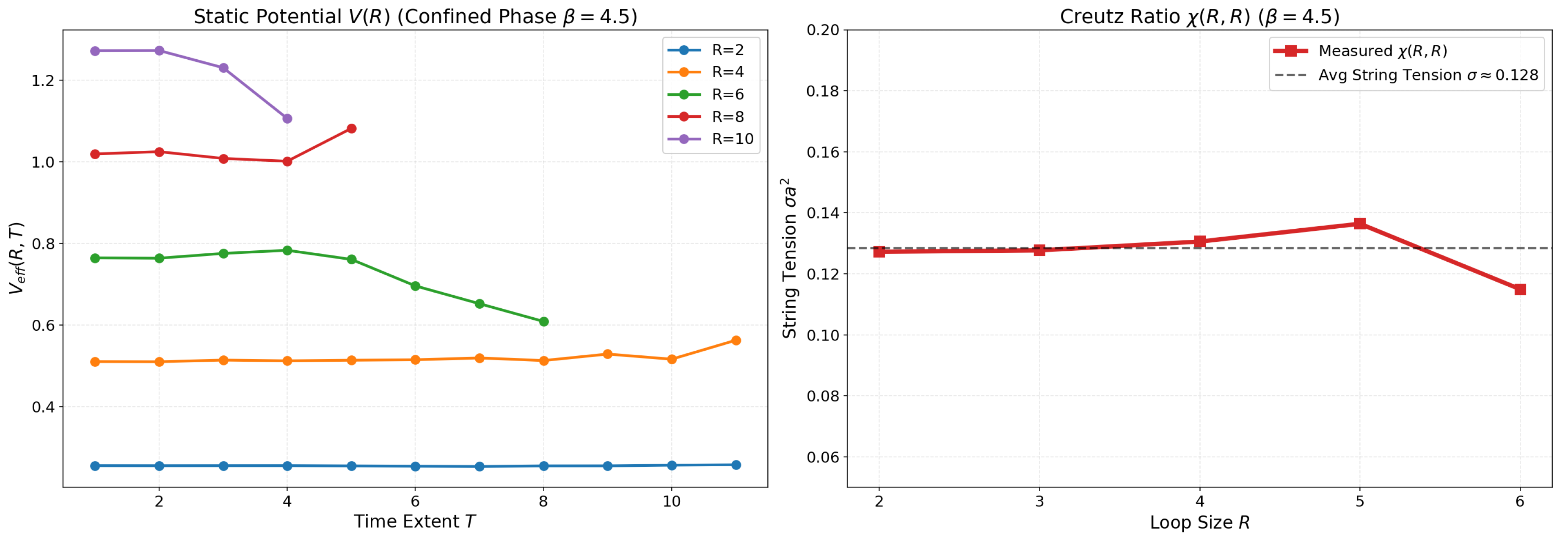
Using our FFM sampler, we successfully resolved the static potential across two distinct physical regimes (Figure 4). The comparison reveals that FFM correctly captures the expected -dependence of confinement observables:
- Strong Coupling (): The system exhibits harsh confinement characteristics. The potential rises steeply (), and Wilson loop signals decay rapidly, reflecting a "stiff" gauge field.
- Scaling Regime (): As the system approaches the continuum limit, the string tension softens significantly to . Remarkably, the model preserves the linear confining potential even in this weak coupling limit, consistent with confinement in 2D compact U(1) across couplings.
A striking feature of the static potentials is the Ground State Dominance. The flatness of effective potential plateaus suggests early plateau behavior / limited excited-state contamination within the accessible T-window for loop sizes with reliable signal.
4.4. Multiscale Sensitivity (ERF Analysis)
To probe how FluxUNet aggregates information across length scales, we computed the Effective Receptive Field (ERF) by measuring the sensitivity of representative internal activations to localized perturbations of the input flux field (Figure 5). The ERF maps reveal a clear separation between shallow, predominantly local processing and deep, globally aggregated processing:
- Local sensitivity (short-range features). In early and intermediate layers, the ERF is sharply localized: the response is concentrated in a compact neighborhood around the perturbed site. This indicates that these layers primarily encode short-range structure, such as local plaquette-angle fluctuations and short-wavelength textures. Such locality is consistent with the fact that many thermodynamic contributions are governed by local statistics, and it provides an inductive bias that avoids unnecessarily entangling distant regions when learning microscopic structure.
- Global sensitivity (long-range features). In the bottleneck layer, the ERF becomes broad and diffuse, indicating that deep features depend on information distributed across the lattice. This pattern is consistent with the network forming global summaries that cannot be inferred from a small patch alone. In particular, sector-dependent structure on a torus (e.g., correlations tied to the total-flux sector Q or other global modes) is inherently nonlocal; representing such effects requires access to long-range context. We emphasize that ERF demonstrates capacity for global dependence, not that the network explicitly computes Q.
4.5. Generalization to Spatial -Conditioning
Standard algorithms typically require re-thermalization or careful annealing for every new potential landscape. In contrast, our model—trained with Spatial -Conditioning—exhibits a qualitative zero-shot response to unseen conditions. To demonstrate this, we evaluate the model on a "Dipole Trap" configuration (Figure 6) without any retraining. We engineer a spatial coupling profile with a vacuum background () and two localized "hot spots" (). We then compute the local magnetic flux density directly from the generated plaquettes:
where is the principal branch of the plaquette angle.
The results reveal a sharp statistical separation: the model consistently generates a concentration of positive flux () in one trap and negative flux () in the other. This emergence of a conjugate pair is not random; it allows the system to satisfy the global topological neutrality of the torus () while entropically localizing the necessary fluctuations within the low-stiffness regions where the energetic cost is minimal (). This behavior is consistent with the network having learned a local conditional dependence . This represents a functional capability beyond standard algorithms: the model can simulate domain walls and flux defects zero-shot, whereas standard HMC would typically require running a new chain for every variation in the profile.
5. Discussion
Dual Flux Transformation
Our results suggest that, in 2D compact at large , topology-sensitive slowing down is severe for standard link-based HMC on accessible timescales, whereas operating in gauge-invariant flux (plaquette-angle) variables yields proposals with markedly improved mixing for topology-sensitive observables. This performance leverages the factorization of the action in the dual basis (Section 2), which effectively decouples the local dynamics.
Similarly, the “Relax-and-Project” mechanism (Section 3.3) ensures global topological validity without restricting the local generative freedom. We then wrap these proposals in an Independent Metropolis–Hastings (IMH) step using an estimated proposal density (via a stochastic trace/divergence estimator). While the stochastic estimator precludes strict detailed balance, our validation confirms that the model, operating in the transformed dual basis, achieves high fidelity, empirically reproducing sensitive thermodynamic, confinement, and topology-related observables to high accuracy. We note that the current implementation reflects a practical compromise between training throughput and numerical precision; further gains in observable fidelity may be achievable with higher-precision arithmetic at the cost of increased training time.
Sampling Efficiency.
A central empirical advantage of FFM is its robust topological mixing. As detailed in Section 4.2 (Table 1), the HMC baseline exhibits extremely large and unstable integrated autocorrelation times for Q, consistent with non-ergodic behavior. In contrast, the conditional FFM sampler maintains across the tested values. This “near-i.i.d.” behavior suggests that the FFM proposal distribution has strong phase-space overlap across the relevant topological structure, allowing the chain to decorrelate in a small number of steps. Although the ESS gain varies by observable, we emphasize that our sampling method can be easily parallelized on modern GPUs to achieve superior performance.
Local Topological Control
The Statistical Dipole Trap experiment demonstrates the utility of Spatial -Conditioning. The ability to spontaneously nucleate conjugate flux concentrations solely through spatially varying profiles is consistent with the model having learned the local conditional statistics of the theory. Rather than treating the inverse coupling as a global scalar, the network utilizes it as a dynamic background field, enabling zero-shot qualitative control over the vacuum structure. As discussed in Section 2, a single trained model samples a continuous range of , amortizing training cost across the tested interval and yielding practical efficiency gains significantly greater than single-point ESS comparisons imply.
Theoretical Boundaries: Dimensionality and the Bianchi Constraint
A rigorous assessment must acknowledge the dimensional boundaries of this approach. The efficacy of the dual flux representation described here relies on the "2D Privilege": in two dimensions, plaquettes tile the plane without enclosing 3-volumes. Consequently, the dual variables are free from local geometric constraints.
In 3D and 4D, however, fluxes live on the faces of elementary cubes. They must satisfy a nontrivial local geometric constraint (discrete Bianchi identity) up to integers. Naive independent sampling in 4D would violate this consistency, leading to non-physical states. Therefore, FFM is not claimed as a universal solution for 4D Gauge Theory in its current form, but rather as a competitive alternative for 2D Compact U(1). Within this domain, it provides a highly efficient mechanism for mitigating critical slowing down in the calculation of topological observables.
Scaling Behavior
We validate FFM on lattices up to (Appendix D). Thermodynamic fidelity (energy density MAE ) and topological susceptibility scaling remain robust at larger volumes. The acceptance rate decreases as expected for independent proposal methods in higher-dimensional phase spaces (7– at vs. 50– at ), while topological autocorrelation remains . Confinement observables, including string tension extraction via Creutz ratios, remain stable, confirming that the physics fidelity of the method scales with system size.
6. Conclusion
We have presented Flux-Space Flow Matching (FFM), a framework that resolves topological freezing in 2D Compact LGT. By lifting the dynamics to the gauge-invariant dual flux representation, we diagonalize the interaction and render sampling tractable. Combined with a “Relax-and-Project” paradigm, FFM yields an IMH-corrected kernel achieving a improvement in topological tunneling rates over HMC. Additionally, Spatial -Conditioning enables zero-shot synthesis of topological defects. Our results suggest that scalable neural sampling requires architectures that respect the native geometric structure of the theory.
Appendix A. Validity of Direct Plaquette Generation in D=2
Appendix A.1. Discrete Variables
Let be a 2D square lattice. Link variables are on oriented edges, parameterized as with . The plaquette variable on an elementary face is
Equivalently, in terms of angles,
where is the forward difference operator.
Appendix A.2. Absence of Local Bianchi Constraints in D=2
On a lattice, the Bianchi identity is the vanishing of the exterior derivative of the 2-cochain : , where is a 3-cochain evaluated on elementary 3-cells (cubes). In , there are no 3-cells; hence the condition is vacuous. Therefore, unlike , there is no local geometric consistency constraint coupling neighboring plaquettes.
Appendix A.3. Local Surjectivity (Constructive Validity on a Patch)
Consider any simply connected local patch (e.g., a receptive-field-sized region) with open boundary. Because has no nontrivial 2-cycles, , so every 2-cochain is exact. Concretely, one may explicitly construct links realizing an arbitrary plaquette field on by an axial-gauge choice. For example, set
then the plaquette constraint reduces to . Fix on the bottom boundary (e.g., ) and define recursively for ,
This yields a valid link configuration on reproducing exactly the prescribed plaquettes. Hence, locally the map is surjective: arbitrary local plaquette fields correspond to some underlying links.
Appendix A.4. Global Topology on the Torus T2
Our simulations use periodic boundary conditions, so the lattice is topologically a torus. In this case , and plaquette configurations decompose into topological sectors characterized by an integer total flux (first Chern number). To state this without ambiguity from branch cuts, it is convenient to work with a real-valued lift: choose integers such that
Thus, the only constraint on plaquettes imposed by the torus topology is the quantization of the total flux Q. In contrast, there are also two global holonomies (Wilson/Polyakov loops along the two non-contractible cycles) which are not determined by plaquettes, i.e. they are global degrees of freedom required to reconstruct links but do not constrain the local plaquette field.
Appendix A.5. Conclusion
In , the absence of local Bianchi constraints implies that the plaquette field behaves locally as an unconstrained scalar field on faces, justifying direct generative modeling of . Global topology only induces an integer-valued total-flux sector label on ; no local geometric consistency constraints analogous to are present.
Appendix B. Training Data Generation (Local Metropolis, L = 48)
To generate the training corpus used in Section 3.2, we run massively parallel persistent local Metropolis updates on the link-angle variables () of a 2D periodic lattice. Updates use a checkerboard (even/odd) scheme and a symmetric uniform proposal with ; accept/reject follows the standard Metropolis rule for the Wilson action at the chain’s fixed coupling .
Configuration and schedule.
We evolve persistent chains in parallel on GPU at lattice size . Each chain is assigned a fixed coupling sampled as a random permutation of , yielding broad coverage of weak-to-strong coupling within each saved batch. Chains are initialized from i.i.d. random link angles .
Warmup, thinning, and storage.
We perform warmup sweeps. We then save dataset chunks, separated by sweeps. Each chunk stores FP32 real-channel link embeddings with , together with the corresponding .

Table A1.
Key hyperparameters for the local-Metropolis data generator.
| Lattice size | |
| Batch size (parallel chains) | |
| range (per batch) | (permuted linspace) |
| Proposal amplitude | |
| Warmup sweeps | |
| Sweeps between saves | |
| Number of saved chunks | |
| Output format | FP32: and |
Appendix C. Supplementary Fidelity Checks
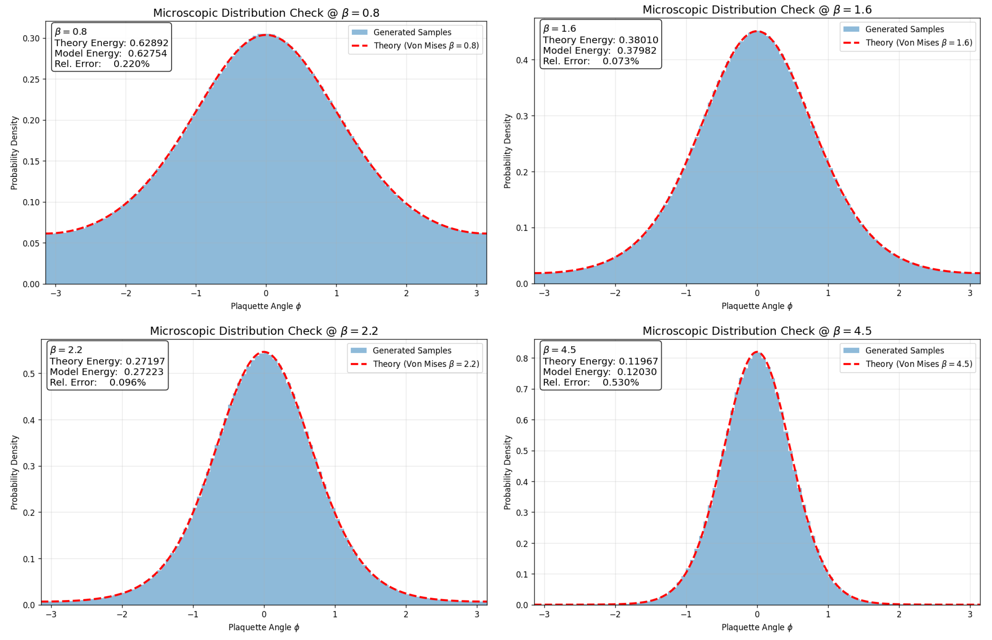
To further substantiate the high fidelity of the generative model, we compare the generated Action Density against the theoretical Von Mises distribution (Figure A1). The near-perfect alignment confirms that the flow matching objective successfully targets the true Boltzmann measure.
Figure A1.
Supplementary Fidelity Verification. Direct histogram comparison of Generative Samples (Red) vs Theoretical Von Mises Density (Teal) across varying inverse couplings . The tight agreement across the entire range confirms the precision of the learned marginals.
Figure A1.
Supplementary Fidelity Verification. Direct histogram comparison of Generative Samples (Red) vs Theoretical Von Mises Density (Teal) across varying inverse couplings . The tight agreement across the entire range confirms the precision of the learned marginals.
Appendix D. Scaling Validation: L = 64 Lattices
To verify that FFM scales beyond the primary benchmarks, we train and evaluate on lattices ( sites). Training was performed on samples using a single NVIDIA B200 GPU for 20 epochs. This appendix reports key fidelity checks demonstrating that the method’s physics accuracy is preserved at larger volumes.
Appendix D.1. Thermodynamic Fidelity
Figure A2 shows the energy density across . The model achieves MAE , comparable to the result (MAE ).
Figure A2.
Energy density check for . MAE confirms thermodynamic fidelity scales with lattice size.
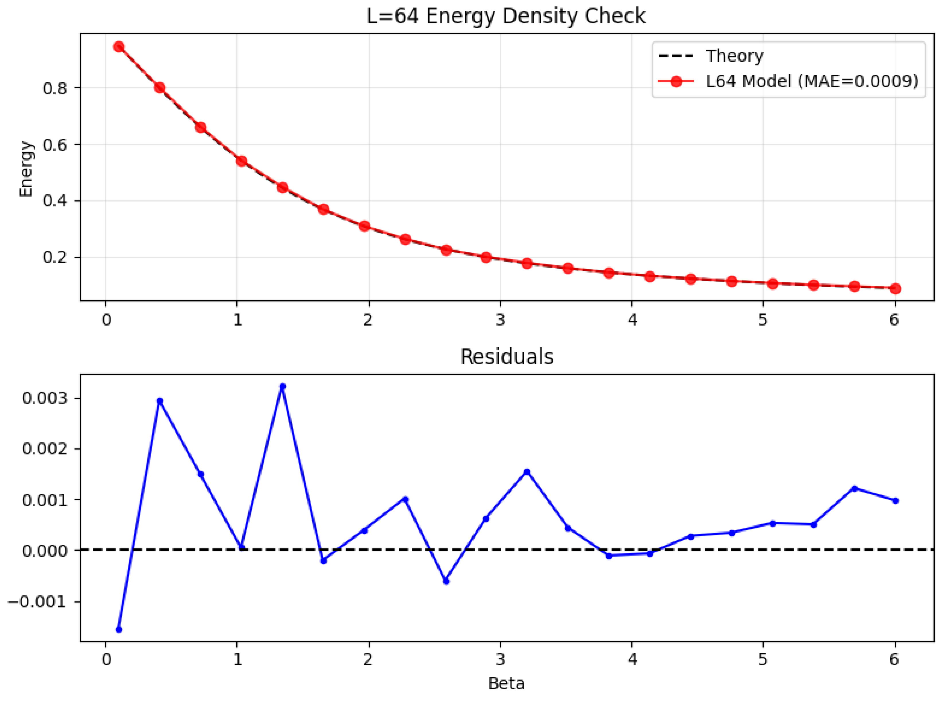
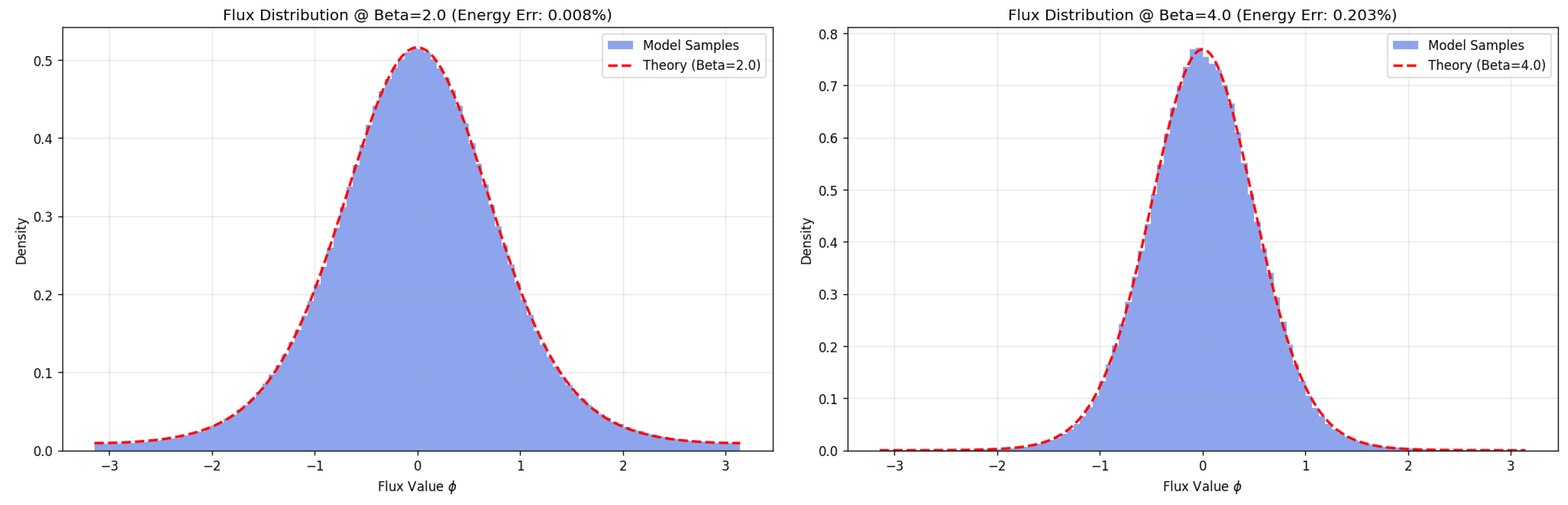
Figure A3 further validates the marginal flux distributions at representative values. At , the model achieves an energy error of just , demonstrating exceptional precision in the intermediate coupling regime.
Figure A3.
Von Mises distribution comparison for at (left, error) and (right, error). The tight alignment confirms the model learns the correct Boltzmann statistics.
Figure A3.
Von Mises distribution comparison for at (left, error) and (right, error). The tight alignment confirms the model learns the correct Boltzmann statistics.
Appendix D.2. Topological Susceptibility
Figure A4 confirms scaling, with values consistently above the non-compact perturbative limit due to vortex contributions.
Figure A4.
Topological susceptibility scaling for . The power-law is preserved.
Appendix D.3. Confinement Diagnostics
Figure A5 shows the static potential and Creutz ratios at . The string tension is consistent with the result at the same coupling (, see Figure 4), and plateaus remain stable for .
Figure A5.
Static potential (left) and Creutz ratios (right) for at . Average string tension , consistent with the benchmark.
Figure A5.
Static potential (left) and Creutz ratios (right) for at . Average string tension , consistent with the benchmark.
Appendix D.4. Sampling Efficiency
Table A2 reports FFM sampling efficiency at . While acceptance rates are lower than (as expected for independent proposals in larger phase spaces), the topological autocorrelation remains .
Table A2.
FFM sampling efficiency on 2D lattices. Values are mean ± std over three random seeds.
| Acc. | ESS/s | ||
| 2.0 | |||
| 4.0 | |||
| 5.0 | |||
| 6.0 |
Appendix D.5. Conclusion
These results demonstrate that FFM scales successfully from to , with physics fidelity preserved across all diagnostics: thermodynamic observables (MAE ), marginal distributions ( error), topological susceptibility scaling, and confinement behavior (string tension consistent with ). While acceptance rates decrease with increasing volume—an expected limitation of independent proposal methods—the topological autocorrelation remains , consistent with the benchmarks. The successful scaling to suggests that FFM can extend to even larger lattices with appropriate computational resources.
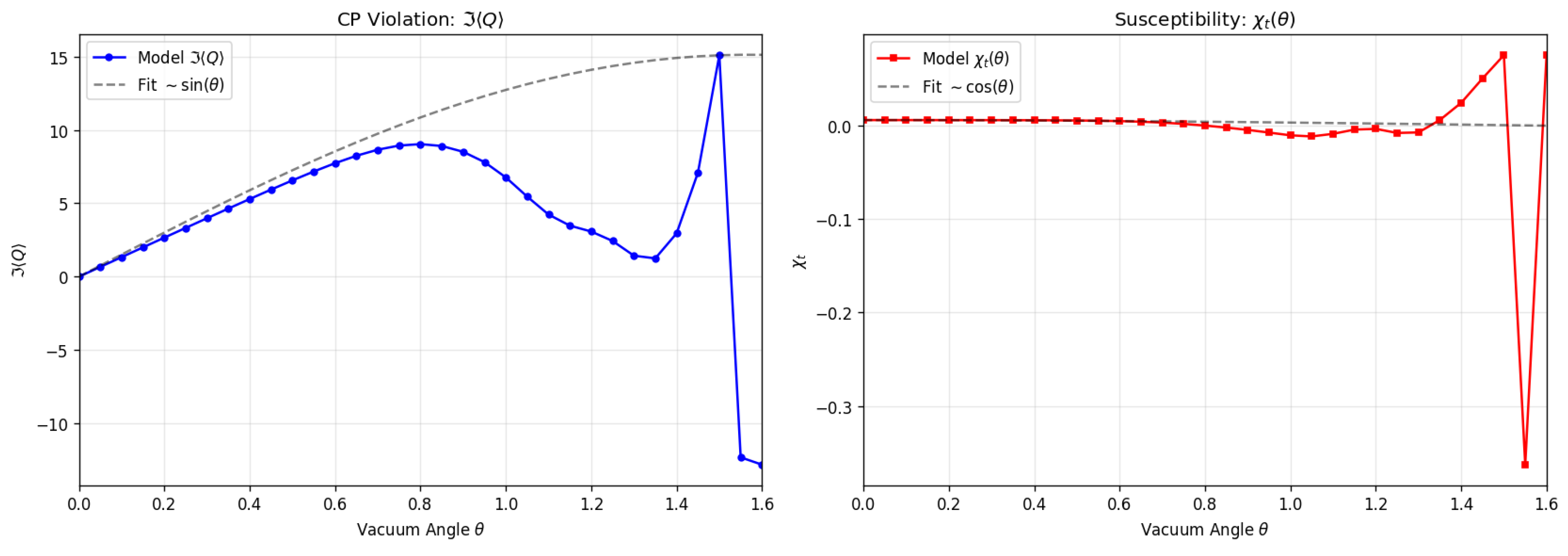
Appendix E. Finite-θ Vacuum Checks via Reweighting
This appendix reports auxiliary finite- diagnostics used to support the fidelity of our learned sampler and analysis pipeline. These measurements are not intended as primary physics claims at large ; rather, they serve as stress tests demonstrating internal consistency within a statistically controlled window (, ).
Appendix E.1. Reweighting Protocol and CP-Even/CP-Odd Extraction
All finite- observables are reconstructed from a ensemble using phase reweighting. We define the complex ratio estimator
Here is the (projected) global topological charge and is its empirical distribution in the ensemble (sector decomposition).
In principle, CP-even observables yield real expectation values, whereas CP-odd quantities are purely imaginary in the CP-symmetric limit. Accordingly, we extract the reported values as:
The explicit in Eq. (A10) removes a small non-physical imaginary component that may arise from finite-statistics asymmetries in the empirical .
Figure A6.
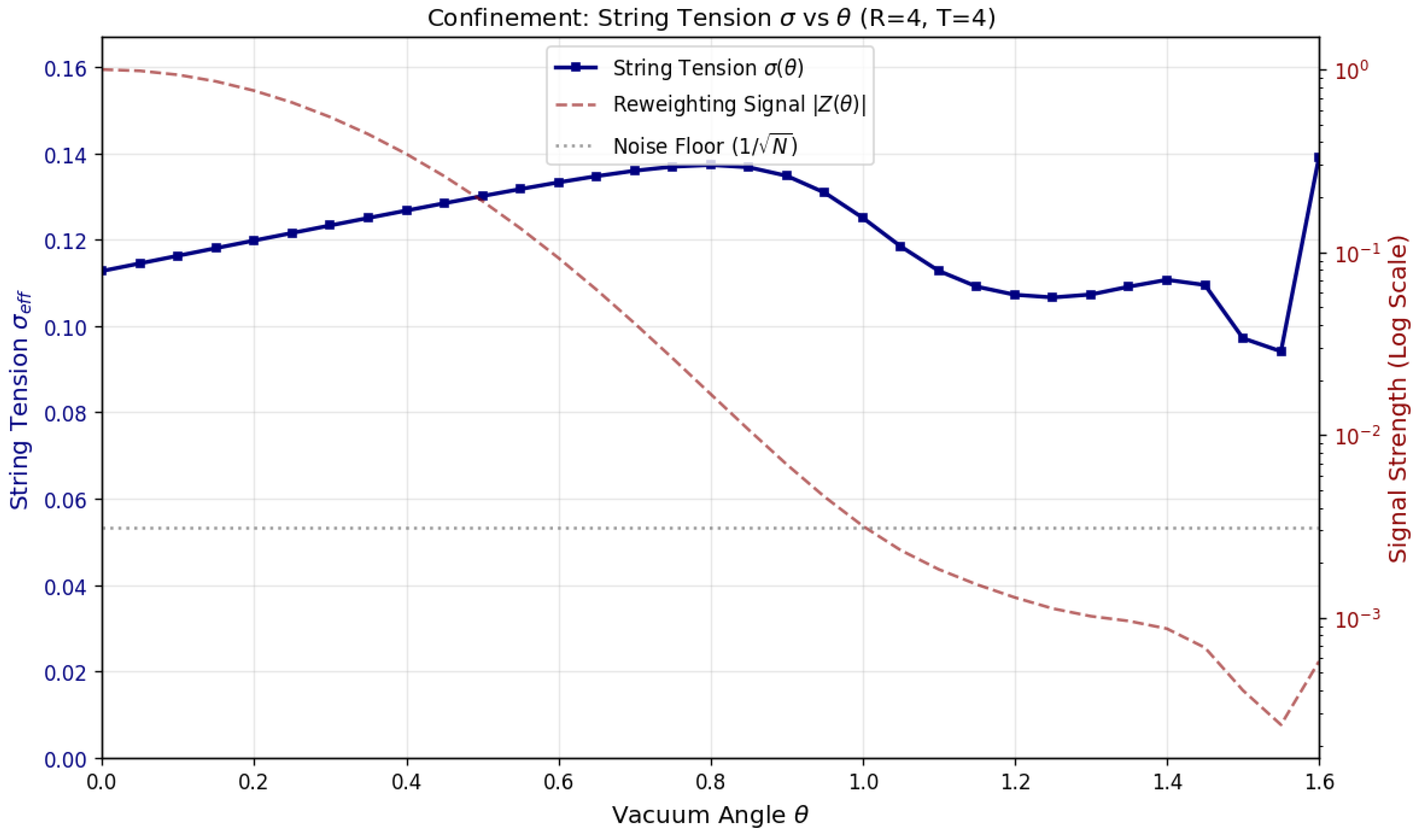
Reweighting signal strength and noise floor, overlaid with effective string tension . The signal crosses the noise floor near .
Figure A6.
Reweighting signal strength and noise floor, overlaid with effective string tension . The signal crosses the noise floor near .
Appendix E.2. Analysis Window, Noise Floor, and Interpretation Scope
The reweighting denominator magnitude decays rapidly with due to phase cancellations across topological sectors. Once becomes comparable to the statistical noise scale , ratio estimators may become noise-dominated and develop spurious structure. For completeness, the measured topological-charge statistics for this run are:
For clarity, we therefore refer to the reported range as an analysis window rather than a “trust window”:
Within this window, the sub-interval corresponds to the region where remains at or above the noise floor for the present statistics (Figure A6), and we treat it as the regime in which reweighted estimates are comparatively well-conditioned. By contrast, the region should be interpreted primarily as a numerical stability test of the pipeline under severe phase cancellations, not as a domain for precision finite- physics. In particular, near the upper end (), the reconstruction is strongly noise-dominated, consistent with the observed instability in susceptibility-like diagnostics and in larger-loop observables.
Appendix E.3. Observables Within the Analysis Window
Within the analysis window, we examine four representative quantities:
- 1.
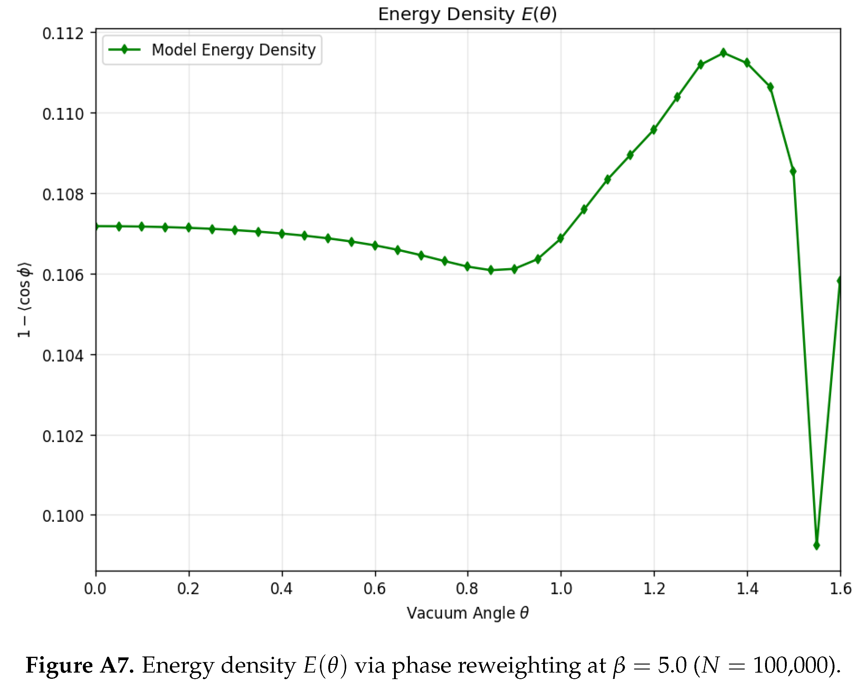
- Energy density : The action density, serving as a bulk thermodynamic check. The reconstructed values remain smooth and vary modestly over (Figure A7).
Figure A7.
Energy density via phase reweighting at ().
- 2.
- Wilson loops for : Probes of confinement at multiple length scales. Small and intermediate loops are broadly stable; larger loops exhibit increased sensitivity near (Figure A8).
- 3.
- Effective confinement proxy : Extracted from a fixed loop (), providing a finite-volume proxy for string tension. Over the majority of the trust window, evolves smoothly (see Figure A6).
- 4.
- CP-odd / topological response: Including and susceptibility-like proxy . These quantities are particularly sensitive to phase cancellations; the visible breakdown near is consistent with the analysis-window boundary (Figure A9).
Figure A9.
CP-odd diagnostics (, ) via reweighting. Instability near marks the trust-window boundary.
Figure A9.
CP-odd diagnostics (, ) via reweighting. Instability near marks the trust-window boundary.
Appendix E.4. Takeaway
These checks show that, despite the rapid decay of the reweighting signal, our learned sampler combined with sector-aware reconstruction yields qualitatively stable finite- observables across . We use these experiments strictly as fidelity tests of the sampling-and-reconstruction pipeline, and we avoid physics-facing interpretation in the noise-dominated regime.
References
- Albergo, M.S.; Kanwar, G.; Shanahan, P.E. Flow-based generative models for Markov chain Monte Carlo in lattice field theory. Physical Review D 2019, 100, 034515. [Google Scholar] [CrossRef]
- Abbott, R.; Albergo, M.S.; Botev, A.; Boyda, D.; Cranmer, K.; Hackett, D.C.; Kanwar, G.; et al. Normalizing flows for lattice gauge theory in arbitrary space-time dimension. arXiv 2023, arXiv:2305.02402. [Google Scholar] [CrossRef]
- Komijani, J.; et al. Super-resolving normalising flows for lattice field theories. SciPost Physics 2026, 19, 077. [Google Scholar]
- Kanwar, G.; Albergo, M.S.; et al. Equivariant flow-based sampling for lattice gauge theory. Physical Review Letters 2020, 125, 121601. [Google Scholar] [CrossRef] [PubMed]
- Albergo, M.S.; Boyda, D.; Hackett, D.C.; Kanwar, G.; et al. Introduction to Normalizing Flows for Lattice Field Theory. arXiv 2021, arXiv:2101.08176. [Google Scholar] [CrossRef]
- Favoni, M.; Ipp, A.; Müller, D.; Schuh, D. Lattice Gauge Equivariant Convolutional Neural Networks. Physical Review Letters 2022, 128, 032003. [Google Scholar] [CrossRef] [PubMed]
- Rezende, D.J.; Mohamed, S. Variational Inference with Normalizing Flows. International Conference on Machine Learning, 2015. [Google Scholar]
- Bander, M.; Itzykson, C. Quantum-field-theory calculation of the two-dimensional Ising model correlation function. Physical Review D 1977, 15, 463. [Google Scholar] [CrossRef]
- Savit, R. Duality in field theory and statistical systems. Reviews of Modern Physics 1980, 52, 453. [Google Scholar] [CrossRef]
- Lipman, Y.; Chen, R.T.; Ben-Hamu, H.; Nickel, M.; Le, M. Flow matching for generative modeling. arXiv 2022, arXiv:2210.02747. [Google Scholar]
- Song, Y.; Sohl-Dickstein, J.; Kingma, D.P.; Kumar, A.; Ermon, S.; Poole, B. Score-Based Generative Modeling through Stochastic Differential Equations. International Conference on Learning Representations 2021.
- Gerdes, M.; de Haan, P.; Bondesan, R.; Cheng, M.C.N. Non-Perturbative Trivializing Flows for Lattice Gauge Theories. arXiv 2024, arXiv:2410.13161. [Google Scholar]
- Rahaman, N.; Baratin, A.; Arpit, D.; Draxler, F.; Lin, M.; Hamprecht, F.; Bengio, Y.; Courville, A. On the spectral bias of neural networks. International Conference on Machine Learning 2019, 5301–5310. [Google Scholar]
Figure 2.
Training Fidelity and Convergence. Evolution of the Action Density during training using the adaptive dopri5 solver. The model rapidly equilibrates to the target energy density, demonstrating efficient and precise learning of the bulk thermodynamics.
Figure 2.
Training Fidelity and Convergence. Evolution of the Action Density during training using the adaptive dopri5 solver. The model rapidly equilibrates to the target energy density, demonstrating efficient and precise learning of the bulk thermodynamics.
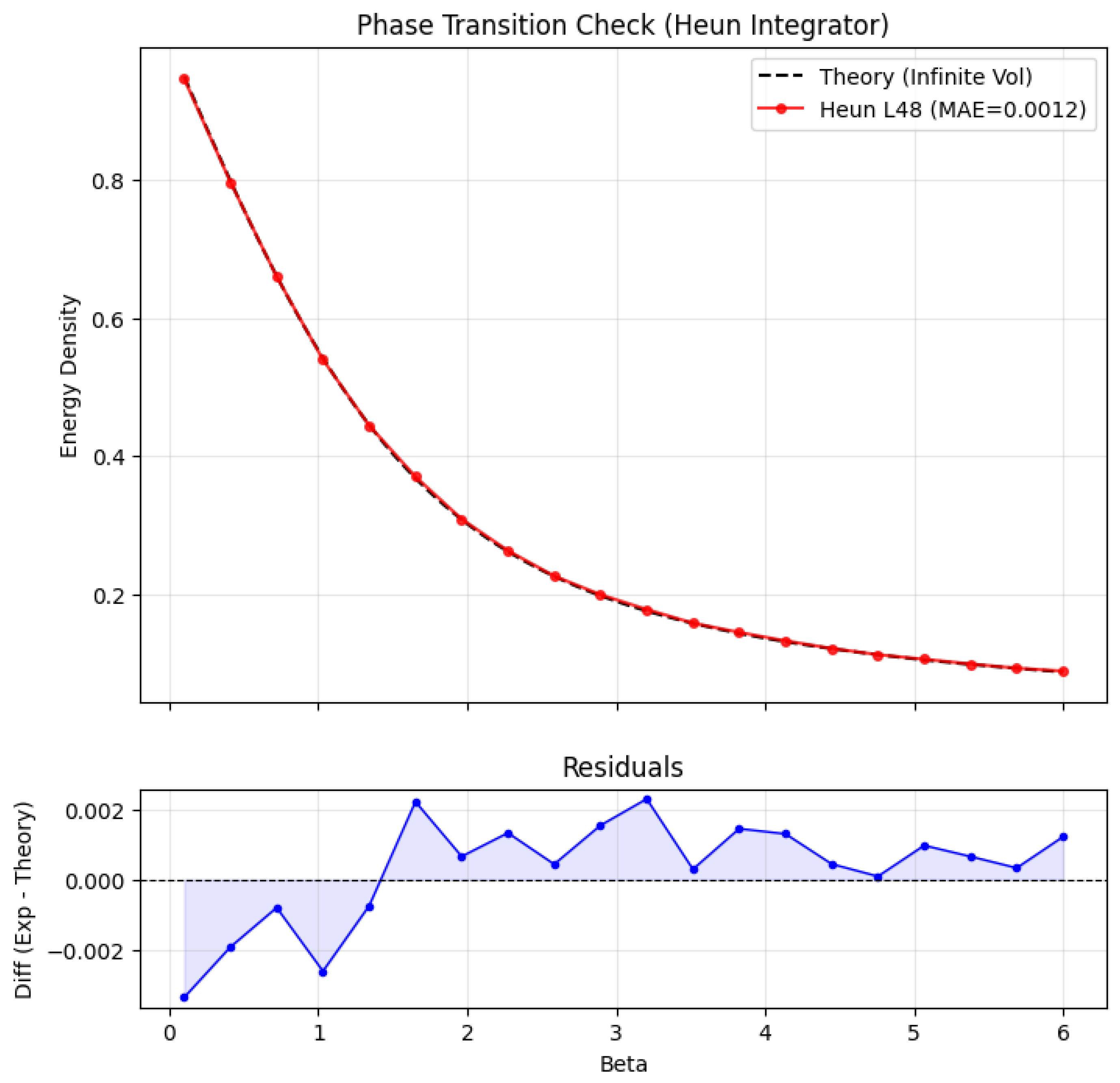
Figure 3.
Topological Susceptibility Scaling. (Left) Log-log scaling of confirms the expected power-law behavior . (Right) The product converges towards but remains consistently above the non-compact perturbative limit (, Dashed), quantitatively isolating the non-perturbative vortex contribution surviving in the continuum limit.
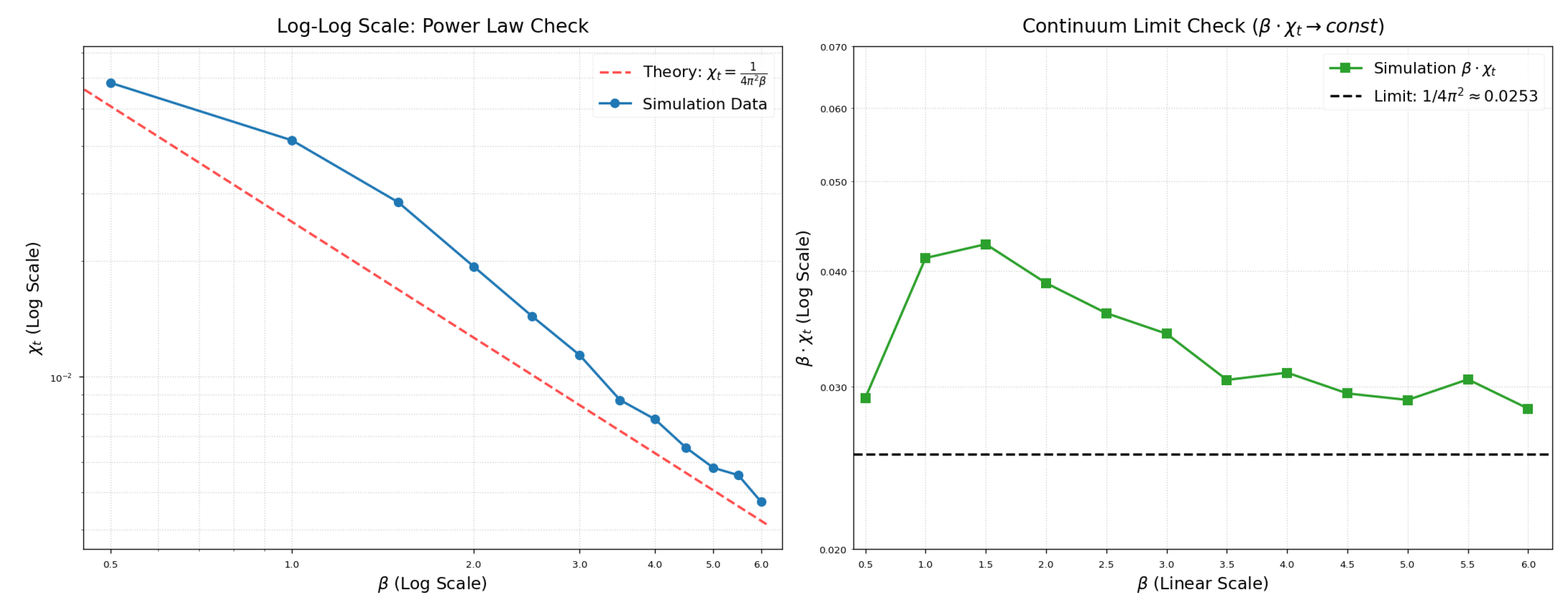
Figure 4.
Static Potential Analysis. (Left) and Creutz Ratios (Right) for Strong Coupling (, Top) and Scaling Regime (, Bottom). While the strong coupling signal decays rapidly (stable up to ), the scaling regime admits reliable potential extraction up to , confirming that the model captures the correct renormalization of the string tension across regimes.
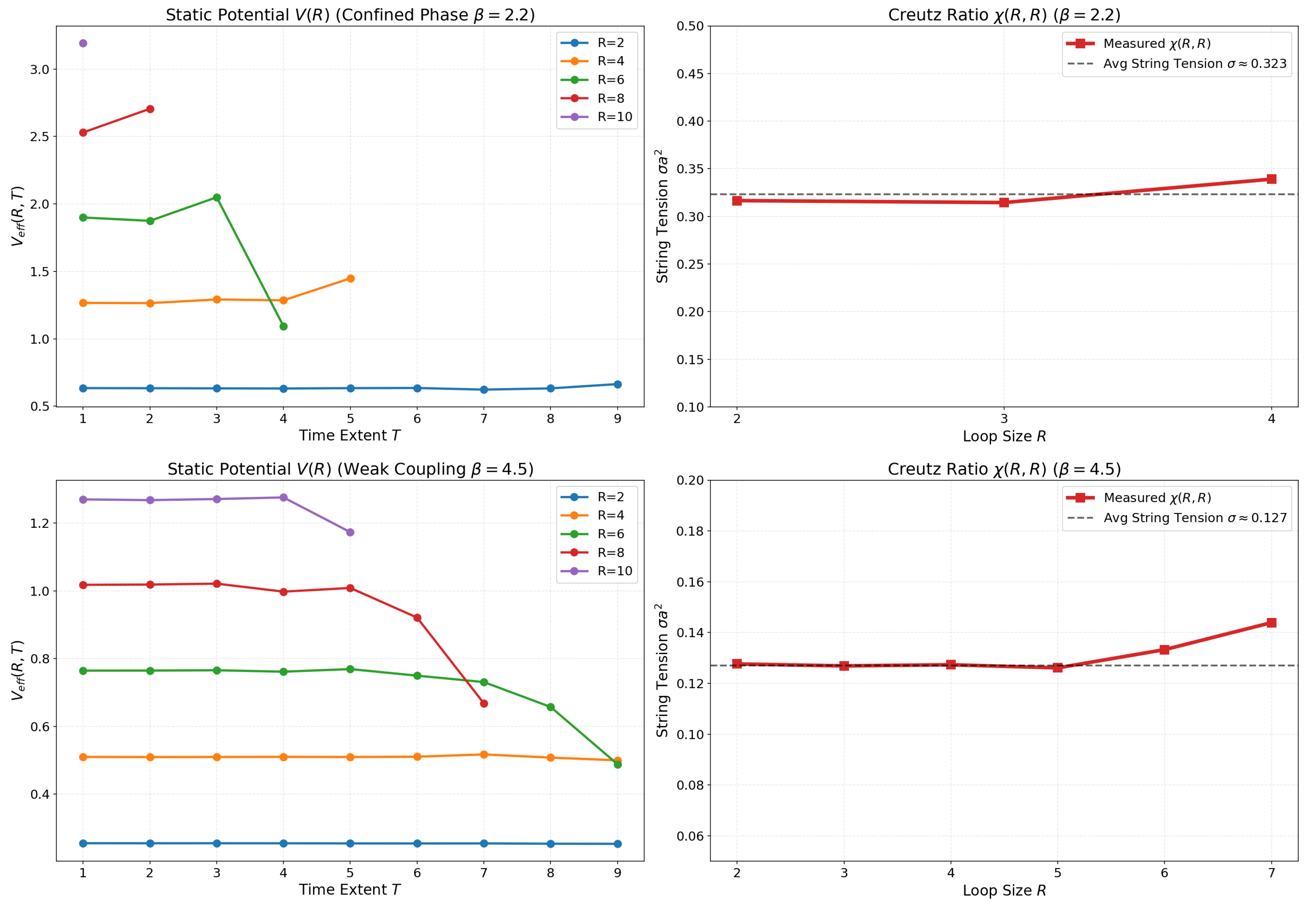
Figure 5.
Structural Scale Separation. Effective Receptive Field (ERF) analysis of the FluxUNet. ERF indicates predominantly local sensitivity in shallow paths and broader/global sensitivity in the bottleneck, consistent with a multiscale representation.
Figure 5.
Structural Scale Separation. Effective Receptive Field (ERF) analysis of the FluxUNet. ERF indicates predominantly local sensitivity in shallow paths and broader/global sensitivity in the bottleneck, consistent with a multiscale representation.
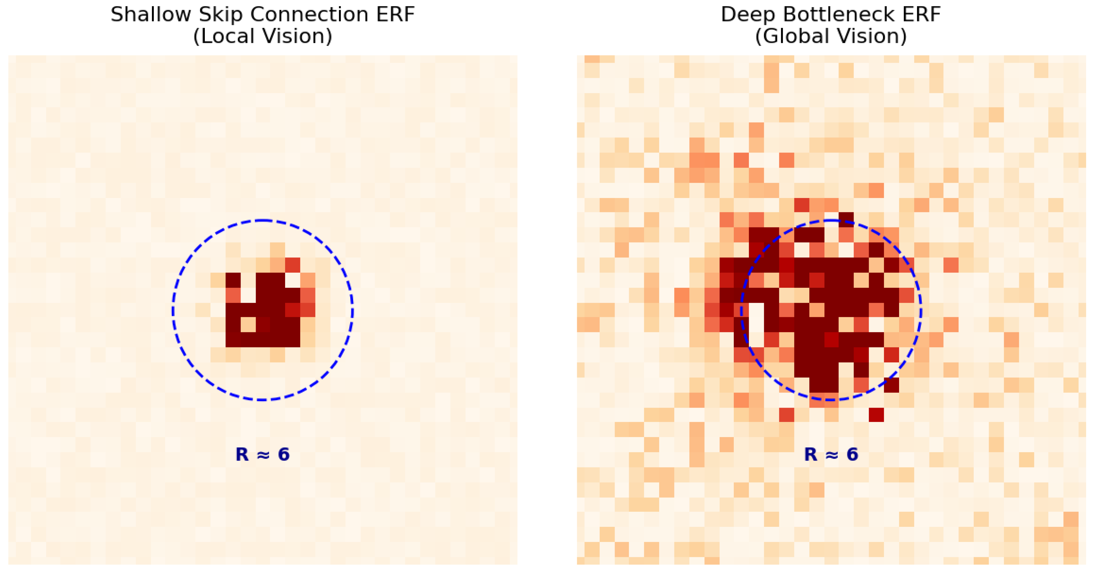
Figure 6.
Zero-Shot Generalization. We engineer a spatial coupling profile () with two localized "hot spots". Using Classifier-Free Guidance (), the model spontaneously generates a Vortex () and Anti-Vortex () pair significantly more often than random chance, confirming the ability to manipulate global topology via local boundary conditions.
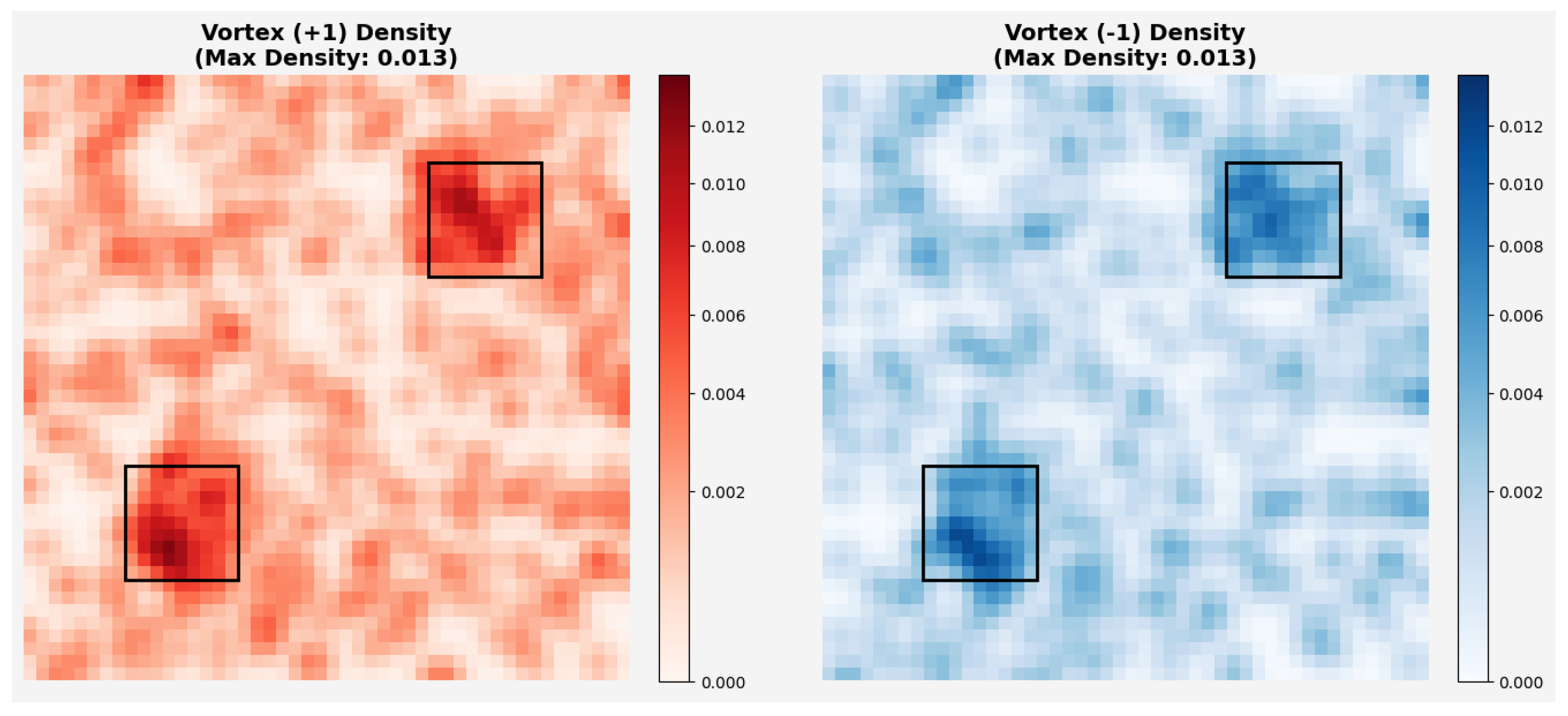
Table 1.
Sampling efficiency on 2D gauge theory (). We denote the integer total flux (topological charge) by Q, and measure its autocorrelation time , together with wall-clock throughput (ESS/s) and MH acceptance rate. Values are mean ± std over three random seeds.
Table 1.
Sampling efficiency on 2D gauge theory (). We denote the integer total flux (topological charge) by Q, and measure its autocorrelation time , together with wall-clock throughput (ESS/s) and MH acceptance rate. Values are mean ± std over three random seeds.
| HMC (baseline) | FFM (our model) | |||||
|---|---|---|---|---|---|---|
| 2.0 | ||||||
| 4.0 | ||||||
| 5.0 | ||||||
| 6.0 | ||||||
Note: All experiments were run on a single GPU using the same implementation and software stack. FFM uses one trained conditional model shared across all , whereas HMC requires separate thermalization (and typically retuning) when moving in parameter space. At low , reduced FFM ESS/s is a compute-cost issue (ODE solve) rather than a mixing issue, since remains .
Disclaimer/Publisher’s Note: The statements, opinions and data contained in all publications are solely those of the individual author(s) and contributor(s) and not of MDPI and/or the editor(s). MDPI and/or the editor(s) disclaim responsibility for any injury to people or property resulting from any ideas, methods, instructions or products referred to in the content. |
© 2026 by the authors. Licensee MDPI, Basel, Switzerland. This article is an open access article distributed under the terms and conditions of the Creative Commons Attribution (CC BY) license (http://creativecommons.org/licenses/by/4.0/).
Copyright: This open access article is published under a Creative Commons CC BY 4.0 license, which permit the free download, distribution, and reuse, provided that the author and preprint are cited in any reuse.


