
Submitted:
22 January 2026
Posted:
23 January 2026
You are already at the latest version
Abstract
Accurately capturing the interaction between fluid motion, chemical reactions, and electric fields is essential for understanding flame behavior in advanced combustion systems relevant to propulsion, energy conversion, and emissions control. In this work, we present a two-dimensional computational framework in cylindrical coordinates for simulating laminar non-premixed flames with electrostatic coupling representative of weakly ionized plasma-assisted combustion environments. The solver employs a high-order compact finite difference scheme for spatial discretization, enabling improved resolution of steep gradients commonly observed in reacting flows, together with a fourth-order temporal integration method to ensure numerical stability and accuracy. Detailed combustion chemistry is incorporated through a steady flamelet formulation, providing an efficient yet robust description of chemical kinetics within the CFD framework. To account for electric field-assisted effects in a simplified and physically consistent manner, the governing equations are extended to include Poisson’s equation for the electric potential and transport equations for one positively and one negatively charged species, assuming a weakly ionized regime in which neutral species dominate the flow dynamics. Electric field effects are modeled by solving species continuity equations for one positively charged and one negatively charged species, coupled with Poisson’s equation for the electric potential to obtain a self-consistent electric field. The resulting electrostatic and plasma-induced effects enter the governing equations through explicit source terms in the momentum and energy equations, accounting for electric body forces and Joule heating for weakly ionized plasma. A systematic parametric study is conducted using a canonical co-flow methane–air diffusion flame to examine the influence of flow conditions and combustor geometry. The results show that plasma forcing leads to a noticeable increase in flame length, as identified by extended OH and CH radical distributions. This behavior is attributed to a combination of electric-field-driven charged species drift, enhanced convective transport, and localized Joule heating, which collectively modify scalar transport and delay radical recombination along the axial direction. Overall, the proposed high-order framework provides a validated and computationally efficient tool for high-resolution simulation of chemically reacting flows with weak plasma coupling, offering new insight into the role of electric fields in laminar non-premixed flame dynamics.
Keywords:
laminar diffusion flame
; flamelet modeling
; electrodynamics
; electric field-flame interaction
1. Introduction
The accurate prediction of flame dynamics in complex flow configurations remains a pivotal challenge in the design and optimization of modern combustion systems, including gas turbines, aero-engine combustors, and next-generation energy conversion devices [1,2]. These systems often operate under conditions where intricate couplings between fluid dynamics, detailed chemical kinetics, and external forcing mechanisms dictate performance, stability, and emission characteristics. Among the promising strategies for active combustion control, the application of plasma-assisted combustion has gained significant interest due to its non-intrusive nature and potential to extend flammability limits, enhance stabilization, and reduce pollutant formation [3,4]. At the core of this phenomenon lies the interaction between an imposed or self-induced electric field and the naturally occurring charged species (ions and electrons) generated through chemi-ionization processes within the flame front [5]. This interaction gives rise to electrostatic forces and localized heating, which can modify local flow fields, scalar transport, and ultimately, the global flame structure and liftoff characteristics [6,7].
Numerically capturing these multiscale, multiphysics interactions presents a formidable computational task. Consequently, reduced-order combustion models have become indispensable for practical engineering simulations. The flamelet concept, originally formalized by Peters [11], has proven particularly powerful for non-premixed combustion. It decouples the detailed chemical kinetics from the flow field by assuming the flame structure resembles that of a one-dimensional laminar flame embedded within the local flow. In this approach, thermo-chemical quantities such as species mass fractions and temperature become unique functions of a few controlling scalars, typically the mixture fraction and a reaction progress variable. This manifold can be pre-computed and tabulated, offering a substantial reduction in computational expense while retaining a high degree of chemical accuracy [12,13]. The flamelet/progress-variable (FPV) formulation [14] has been successfully extended and validated for a wide range of configurations, including lifted and partially premixed flames [15,16]. The integration of electric field effects into such a framework introduces additional layers of complexity. The electric field couples with the flow through the motion of charged particles. Accurate modeling requires not only a suitable description of the ionization chemistry but also the solution of additional transport equations for charged species and Poisson's equation for the electric potential to ensure a self-consistent field [17]. Early models, such as those by Hu et al. [18], often assumed a constant, externally applied electric field, neglecting the crucial feedback of charge separation on the field itself. More recent works have advanced the coupling. For instance, Yamashita et al. [19] solved the Gauss law in simulations of a capillary flame, while Belhi et al. [20,21] incorporated detailed ion transport within a DNS framework, revealing significant modifications to flame stabilization due to electrostatic forces. However, resolving the full set of ion species transport equations within a detailed chemistry framework remains computationally prohibitive for multi-dimensional design studies.
Di Renzo et al. [22] proposed an efficient flamelet progress-variable method tailored for weak electric fields. They reduced the description of charged species transport to just two scalar quantities representing the total positive and negative charge densities. These scalars are transported with source terms, and mobilities averaged from the underlying detailed ionization mechanism, which is pre-processed and stored within the flamelet manifold. This approach allows for the incorporation of complex ionization kinetics without increasing the number of transported species during the computational fluid dynamics (CFD) solution, yielding speedups of up to 40 times compared to detailed ion transport simulations [22]. Their model successfully captured the characteristic "diodic" effect, where flame response differs for positive and negative voltage polarities, and demonstrated the critical role of heavy anions in flame stabilization dynamics.
On the numerical methodology, achieving high spatial accuracy is essential for resolving the sharp gradients in species concentrations, temperature, and electric potential prevalent in flame zones and boundary layers. High-order compact finite difference schemes offer a compelling alternative to traditional second-order methods or spectral techniques [23]. These schemes achieve high formal accuracy (e.g., fifth-order) on compact stencils, providing excellent spectral resolution with favorable stability properties and reduced numerical dissipation, which is crucial for long-time integration and capturing instabilities [24,25]. Their application to combustion simulations, however, has been relatively limited. Dobbins and Smooke [26] employed a compact scheme for unsteady laminar flame calculations, while more recently, Biazar and Mehrlatifan [27] applied it to reaction-convection-diffusion equations. In the context of complex flow geometries, high-order methods are particularly valuable. Hasan and Gross [28] studied the effectiveness of a higher-order-accurate compact finite difference for investigating spatial instabilities in inward radial Rayleigh–Bénard–Poiseuille flows. Haque et al. [29] applied compact finite-difference discretization to flamelet-based scalar transport in laminar flames, where accurate resolution of steep gradients and transport–chemistry coupling is essential. Their results showed that the compact scheme provides enhanced spectral-like accuracy while maintaining numerical stability in the presence of strong convective acceleration. Subsequent studies further extended this approach to turbulent flame configurations, demonstrating its capability to capture multiscale interactions between turbulence, scalar transport, and combustion dynamics. The model was validated against benchmark experimental data for a laminar co-flow diffusion flame [30] and employed to conduct a systematic parametric study on the effects of Reynolds number, velocity ratio, and combustor geometry. The results underscored the utility of high-order methods in providing accurate predictions of flame structure and scalar fields. However, this framework did not incorporate any plasma or electric field effects.
A clear need therefore remains for a unified, high-fidelity computational framework that efficiently couples flamelet-based combustion modeling with high-order compact discretization and a physically consistent yet tractable weakly ionized plasma model to enable predictive, high-resolution simulations of plasma-assisted laminar and turbulent flames and to elucidate electric-field effects on flame stabilization, liftoff, and scalar transport.
To address this gap, the present work introduces a novel computational framework for the simulation of weakly ionized plasma-assisted laminar non-premixed flames. The solver is developed in cylindrical coordinates and solves the Navier–Stokes equations coupled with transport equations for positive and negative charged species, along with an electric field solver, and is implemented in Fortran. The fluid dynamics and scalar transport are solved using a high-order accurate compact finite difference scheme, extending the methodology validated in [28,29] to ensure sharp resolution of gradients in velocity, species, and electric potential fields. Combustion chemistry is efficiently incorporated via a steady flamelet/progress-variable approach, where the thermo-chemical state is retrieved from pre-computed tables parameterized by mixture fraction and progress variable. This involves solving transport equations for two representative charge density scalars (PP and MM) and Poisson’s equation for the electric potential, with all necessary properties (mobilities, diffusivities, source terms) being derived from a detailed ionization mechanism and stored within the flamelet manifold. The resulting electric field and charge densities introduce source terms into the momentum and energy equations, accounting for electrostatic body forces and Joule heating. The proposed high-order compact finite difference method for weakly ionized plasma-assisted flamelet transport aims to provide a robust, efficient, and accurate tool for advancing the fundamental understanding and predictive capability of plasma-combustion interactions in laminar diffusion flames.
2. Numerical Model
2.1. Computational Fluid Dynamics Model
2.1.1. Governing Equations
The non-dimensionalized compressible Navier–Stokes equations are solved using a compact finite difference scheme. The governing equations for mass, momentum, energy, and mixture fraction are formulated in conservative vector form in cylindrical coordinates.
Here, Q denotes the state vector defined in Eq. (2). The flux vectors A (=E(1))and B (=E(2)) are given in Eq. (3), while the source term vectors C and D are specified in Eqs. (4) and (5), respectively [9]. The Navier–Stokes equations are non-dimensionalized using the reference density, fuel inflow velocity , reference temperature =300 K, and channel half height . Pressure and gravitational acceleration are scaled by and respectively. The Prandtl number () is set to unity. In the governing equations, the effect of the electric field on charged species transport is introduced through electric drift terms that appear in the convective fluxes. These terms are expressed in non-dimensional form using electric Péclet numbers, where and denote the electric Péclet numbers for positively and negatively charged species, respectively. Each electric Péclet number is defined as the ratio of the characteristic electric drift velocity to the reference flow velocity, . The inclusion of and allows the model to capture the asymmetric response of positive and negative charge carriers to the applied electric field in a physically consistent and computationally tractable manner, which is appropriate for weakly ionized flow conditions.
The source terms represent the net volumetric production of positive and negative charge carriers due to ionization and recombination processes in the weakly ionized plasma. These terms ensure local charge conservation and provide the coupling between charged species transport and the electrostatic field through Poisson’s equation, while avoiding the need for detailed plasma chemistry modeling.
The variables u and v denote the streamwise (r-direction) and wall-normal (z-direction) velocity components, respectively. The static pressure is represented by p, denotes the density, e is the total energy, and Z is the mixture fraction. The total energy e is defined as the sum of the internal energy and the kinetic energy . The term appearing in H arises from the Boussinesq approximation, with the gravitational acceleration acting in the r-direction, as illustrated in Figure 1. [29]
Equations (7) express the stress tensor, with and being the Reynolds number and the dynamic viscosity, respectively. The density in the model is evaluated using the ideal gas law (), where R is the gas constant.
The mixture fraction, Z is dependent on the flow velocities (), density (), and mass diffusivity (). The mass diffusivity for all the species is considered identical (), and is derived using the relation between mass and thermal diffusion, i.e., Lewis number (). The mixture fraction ranges from 0-1, with 0 being oxidizer only flow and 1 being the fuel only flow.
The wall-normal first derivatives of the Navier–Stokes equations are discretized using fifth-order accurate upwind- and downwind-biased compact finite difference schemes [8]. The viscous terms are evaluated with a fourth-order accurate compact finite difference formulation, with coefficients taken from Shukla et al. [31]. The resulting tridiagonal systems are solved using the Thomas algorithm. Temporal integration is performed with a fourth-order Runge–Kutta scheme, where superscripts n and n+1 denote consecutive time levels. Further details of the numerical methodology are provided in Refs. [29].
2.1.2. Electric Field Implementation
The electrostatic potential is governed by the axisymmetric Poisson equation in cylindrical coordinates (r,z), assuming invariance in the azimuthal direction. Under this assumption, the governing equation is written as
Introduce characteristic scales L, φ, for length, potential, and charge density, respectively, and define the dimensionless variables
With these definitions, Eq. (1) becomes
where the dimensionless parameter
In the implementation below, the scales such that λ = 1, so the right-hand side becomes simply −.
Finite Difference Discretization
The dimensionless Poisson equation is discretized on a uniform structured grid in the (r,z) plane. Second-order central finite differences are employed for both the radial and axial diffusion terms. The cylindrical geometry is accounted for explicitly in the radial discretization through the 1/r dependence, resulting in asymmetric coefficients for the neighboring radial nodes.
A standard second order finite difference approximation of equation at an interior grid point (i,j) (2 ≤ i ≤ Nr −1, 2 ≤ j ≤ Nz −1) yields,
where the (dimensionless) coefficients are
Rearranging for , gives the Gauss – Seidel update formula
At each interior grid point, the discretized equation couples the potential at the current node to its four nearest neighbors. The resulting algebraic equation preserves second-order accuracy and reflects the geometric effects inherent to cylindrical coordinates. The discrete form is rearranged to yield a pointwise update expression for the electric potential, which is subsequently used in the iterative solution procedure.
Successive Over-Relaxation (SOR) Method
The resulting system of linear algebraic equations is solved using a Gauss–Seidel-based successive over-relaxation (SOR) method. In this approach, the Gauss–Seidel update is combined with the solution from the previous iteration using a relaxation factor ω, where 1 < ω < 2 . The over-relaxation accelerates convergence by extrapolating the solution toward its steady-state value.
The potential is updated sequentially at all interior grid points, while Dirichlet boundary conditions are enforced by prescribing zero potential along all domain boundaries. Convergence is assessed by monitoring the maximum absolute change in the potential field between successive iterations. The iterative process is terminated once the residual falls below a prescribed tolerance.
2.2. Flamelet Model
The flame dynamics are evaluated using the steady flamelet approach. In this approach the flow field and flame chemistry are decoupled, then the time and space evolution of the temperature and the species concentrations are predicted using the evolution of the mixture fraction, Z. Equation (16)-(20) show the expressions for the steady flamelet model used in this study. Here, in Equation (16) denotes the temperature and the mass fraction of the species, which is evaluated through the integration of and across the Z space. The term represents for a given value of Z and is the probability density function (PDF). As Z ranges from 0 to 1, the β-distribution is used to calculate the PDF shown in Equation 17[32], where, is the gamma function. The terms and are calculated using the variance of the mixture fraction, (Equations 18 and 19) and which must be of positive non-zero value (Equation 20).
The flamelet table is generated using the open-source chemical kinetics code called Cantera. A one-dimensional counter-flow diffusion flame model [33] is considered for the methane-air combustion. This model provides the temperature and the species mass fraction for different values of Z (0 ≤ Z ≤ 1). The mixture fraction in this model can be calculated using the mass fractions of the fuel and oxidizer or through nitrogen mass fraction [34]; Since both these expressions yield similar Z profiles; either of these can be used to calculate Z. The N2-based approach is used in this study to generate the flamelet table [29]
Here, is the mass fraction of N2 at the grid point, is the initial N2 mass fraction in the oxidizer stream, and is the N2 mass fraction in the fuel stream. Figure 1 shows the schematic diagram of the counterflow diffusion flame for flamelet generation and the dependency of temperature and species mass fraction on the mixture fraction (Z) observed from the flamelet table. The specific heat capacity () of the individual species is calculated using the NASA polynomials coefficient [35,36,37], where is the universal gas constant (8.314 J/mol-K), marks the different species, - are the polynomial coefficients and is the temperature in a grid point. The value of the polynomial coefficients are obtained from the GRI-Mech 3.0 thermodynamic database [40].
2.3. Boundary Conditions
The simplified schematic diagram of the 2D combustor domain with boundary conditions are illustrated in Figure 2(a). The co-flow combustor geometry is based on the experimental investigations of McEnally and Pfefferle [39] and Bennett et al. [38]. The experimental study's dimension and flow conditions are also used to validate the developed model. The inner diameter of the fuel inlet (Z=1) is 11.1 mm, which is surrounded by a 0.8 mm thick wall, followed by concentric annular air inlet (Z=0) of 95.2 mm outer diameter and 3.4 mm thick outer wall. The combustion chamber has a diameter (D) of 102 mm with 200 mm in length (L). Fuel and air inlet mass flow rates are specified as 3.608✕10-6 and 8.65✕10-4 kg/s, respectively at 300 K. No-slip wall is considered for the combustor wall. Inflow (Riemann invariants-based non-reflecting condition [40]) and outflow (characteristics-based [41]) conditions are selected for the inlets and outlet, where the reference profiles are prepared using 1D NS equations (Equations 21).
The developed model solves the cylindrical NS equation, which provides the flexibility to conduct numerical studies on both a 2D planar body and a cylindrical computational domain [42]. Adopting the code to solve for 2D planner domain requires setting the radii to be infinitely long. This minimizes the influence of azimuthal components (θ). The flow is considered in the inward radial direction, where the inner and outer radius, is set at 107, and the outer radius, is the sum of and the length of the combustor.
Uniform grid distribution is considered along the r-direction (stream-wise), while grid clustering is employed in z-direction (wall-normal) as presented in Figure 2(b). The analytical relationship applied.
3. Results and Discussion
3.1. Grid Independence (Mesh Convergence) Study
A grid independence study was performed to ensure that the numerical predictions are not influenced by spatial discretization and that the selected mesh provides an adequate balance between accuracy and computational efficiency. Three structured meshes of increasing resolution were considered for the two-dimensional axisymmetric computational domain: a coarse grid with 144×72 cells (Grid-1), a medium grid with 288×144 cells (Grid-2), and a fine grid with 576×288 cells (Grid-3).
The assessment of mesh sensitivity was carried out by comparing the axial centerline temperature profiles obtained using the three grids. Figure 3 illustrates the variation of temperature along the combustor axis for all mesh resolutions. As shown, noticeable deviations are observed between Grid-1 and the finer meshes, particularly in regions characterized by steep temperature gradients near the flame zone. In contrast, the temperature distributions obtained using Grid-2 and Grid-3 are nearly indistinguishable over the entire axial distance, including the peak temperature location and the downstream decay region.
The close agreement between the medium and fine grids indicates that further mesh refinement beyond 288×144 does not lead to a meaningful change in the predicted temperature field. Considering that Grid-3 contains approximately four times more computational cells than Grid-2, while offering negligible improvement in solution accuracy, Grid-2 was selected as the production mesh for all subsequent simulations. This choice ensures grid-independent results while maintaining reasonable computational cost.
3.2. Model Validation
The present numerical model is validated against the well-established axisymmetric laminar methane–air diffusion flame studied by Michael D. Smooke et al., under identical operating and geometric conditions. Figure 4 compares temperature profiles plotted as a function of mixture fraction at axial locations corresponding to those reported in the Smooke study. The present predictions closely reproduce both the peak flame temperature and its location near the stoichiometric mixture fraction, as well as the downstream decay trend, demonstrating excellent agreement with the benchmark results.
In the reference configuration, Smooke et al. [43] considered an unconfined, axisymmetric coflow methane–air diffusion flame at atmospheric pressure. The fuel was injected through a central circular nozzle of radius Ri = 0.2 cm, surrounded by an annular air coflow with an outer radius Ro = 2.5 cm. Both the methane jet and the surrounding air stream entered the domain with uniform axial velocities of approximately 35 cm s⁻¹, yielding a laminar flow regime with a characteristic Reynolds number of Re ≈ 100, based on the fuel-jet diameter and inlet conditions. Detailed transport properties and finite-rate chemistry were employed in the original simulations, providing a stringent reference for validation.
Under these same conditions, the present model captures the temperature–mixture-fraction correlations at multiple axial locations (e.g., 1–2 cm above the burner), with only minor deviations in peak magnitude. This level of agreement confirms the accuracy of the numerical formulation and supports its suitability for predicting laminar non-premixed methane–air diffusion flames under canonical Smooke-type configurations.
3.3. Analysis
Figure 5, Figure 6, Figure 7 and Figure 8 present a comparative visualization of the baseline case (left side of each panel, without plasma forcing) and the plasma-forced case (right side of each panel) in terms of OH radical distribution, temperature, mixture fraction (Z), and H₂O mass fraction. These fields collectively describe the evolution of the reactive zone, heat release, mixing behavior, and product formation, thereby providing a comprehensive picture of the plasma–flame interaction.
In the absence of the electric field (base case), the OH contours show a narrow reaction zone originating near the jet base and extending downstream in a relatively slender and symmetric structure. This behavior is characteristic of a diffusion-controlled flame stabilized primarily by thermal and molecular transport processes. The OH concentration gradually decays along the axial direction, indicating a progressive reduction in reaction intensity as reactants are depleted and the flow expands radially. With the electric applied, the OH field exhibits a noticeable modification in both magnitude and spatial extent. The OH-rich region becomes more pronounced near the base and persists farther downstream compared to the baseline case. This enhancement suggests that plasma forcing promotes radical production and sustains active chemistry over an extended region. This behavior is consistent with plasma-assisted pathways that generate additional active species and accelerate chain-branching reactions, thereby reinforcing the reaction zone even under conditions where purely thermal chemistry would weaken.
The temperature contours further corroborate this interpretation. In the baseline case, the high-temperature core remains confined close to the jet axis and decays gradually downstream. When plasma forcing is introduced, the temperature field shows an intensified and more elongated high-temperature region. The increase in both peak temperature and axial penetration of elevated temperatures indicates that plasma forcing contributes additional energy to the system and enhances overall heat release. Importantly, the spatial correspondence between elevated temperature and enhanced OH concentration highlights the strong coupling between chemical activity and thermal transport in the plasma-assisted case. The influence of plasma forcing on scalar transport is evident from the mixture fraction (Z) contours. Without plasma forcing, the Z field shows a relatively smooth axial decay with limited radial spreading, reflecting mixing dominated by the underlying flow field. In contrast, the plasma-forced case exhibits a redistribution of Z near the core region, with altered gradients and enhanced axial persistence. This behavior suggests that plasma forcing not only affects chemistry but also modifies the effective mixing characteristics, either through localized heating, electrohydrodynamic effects, or plasma-induced perturbations to the flow.
Finally, the H₂O contours reveal the cumulative effect of plasma forcing on product formation. In the baseline case, H₂O production follows the expected trend of gradual buildup downstream of the reaction zone. With plasma forcing, the H₂O-rich region becomes stronger and extends over a larger axial distance, consistent with the enhanced OH and temperature fields. This increase in product formation provides further evidence that plasma forcing promotes sustained combustion chemistry rather than merely altering local thermal conditions.
Taken together, these results demonstrate that plasma forcing influences the flame or reactive jet through a combination of enhanced radical chemistry, increased heat release, and modified scalar transport. Rather than acting solely as an external energy source, the plasma interacts synergistically with the flow and chemical kinetics, leading to measurable changes in reaction-zone structure and downstream evolution. These findings highlight the potential of plasma forcing as an effective control mechanism for stabilizing and intensifying reactive flows, particularly under conditions where conventional thermal stabilization is limited.
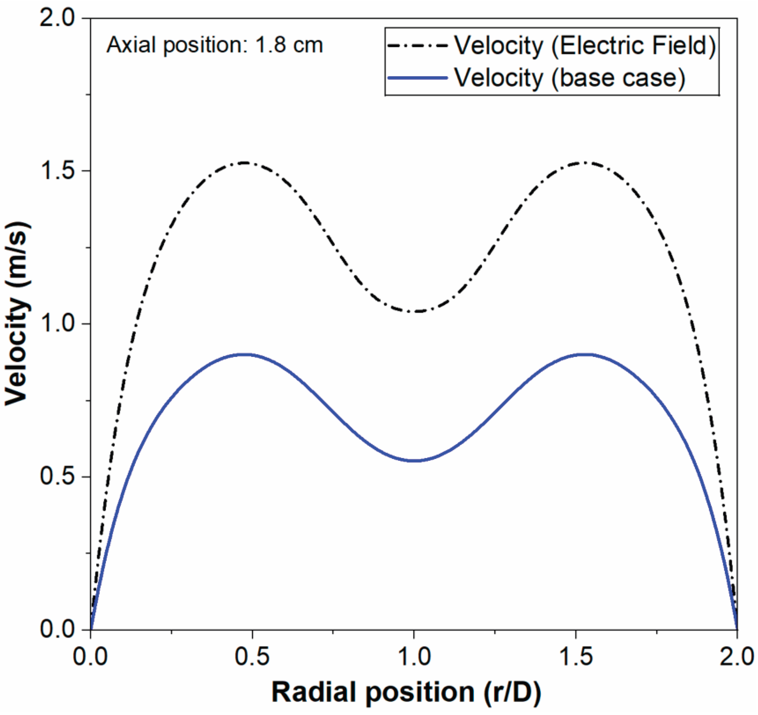
The Figure 9 and Figure 10 present radial velocity profiles at two axial locations (0.5 cm and 1.8 cm), comparing the baseline hydrodynamic case with the electric-field-assisted case.
At the upstream location (axial position = 0.5 cm), both cases exhibit similar double-peaked radial velocity distributions with maxima away from the centerline and zero velocity at the walls (r/D = 0 and 2). The electric-field case shows only a marginal increase in velocity magnitude compared to the base case, while the overall profile shape remains nearly unchanged. This indicates that, close to the inlet, the flow is still primarily governed by inlet momentum and viscous effects, and the electric field induces only a weak perturbation.
At the downstream location (axial position = 1.8 cm), the influence of the electric field becomes much more pronounced. While the baseline case shows significantly reduced velocities due to viscous dissipation and flow development, the electric-field-assisted case maintains substantially higher velocity levels across the entire radial span. The enhancement is especially evident near the off-center peak regions, where the velocity under electric forcing is markedly larger than in the base case. This behavior suggests that the electric body force associated with charged species transport provides sustained flow acceleration downstream, counteracting momentum decay.
4. Conclusions
A high-order compact finite difference framework was developed and applied to simulate weakly ionized electric-field-assisted laminar methane–air diffusion flames in a two-dimensional axisymmetric configuration. The solver couples the compressible Navier–Stokes equations with transport equations for one positively and one negatively charged species and a self-consistent solution of Poisson’s equation for the electric potential, while combustion chemistry is incorporated through a steady flamelet/progress-variable formulation. Fifth-order accurate compact schemes were employed for convective terms, fourth-order compact discretization for viscous terms, and a fourth-order Runge–Kutta method for time integration. Grid-independence was established using three meshes (144×72, 288×144, and 576×288), with the 288×144 grid yielding grid-independent centerline temperature predictions while reducing computational cost by approximately a factor of four relative to the finest grid. Validation against the canonical Smooke laminar methane–air diffusion flame (Re ≈ 100, inlet velocity ≈ 35 cm s⁻¹) demonstrated close agreement in temperature–mixture-fraction profiles, accurately reproducing both peak temperature location near stoichiometric conditions and downstream decay behavior.
Electric-field-assisted simulations showed clear quantitative and qualitative departures from the baseline case. Plasma forcing resulted in an extended OH-rich reaction zone and sustained high-temperature regions over a longer axial distance compared to the hydrodynamic flame. Radial velocity profiles revealed that, while differences near the inlet (x ≈ 0.5 cm) were minimal, electric-field forcing maintained substantially higher velocity magnitudes downstream (x ≈ 1.8 cm), counteracting viscous momentum decay and enhancing convective transport. These coupled effects led to increased H₂O production and delayed radical recombination, consistent with electric-field-driven charge transport and Joule heating. Overall, the results demonstrate that even under weakly ionized conditions, electric fields can significantly alter flame structure, scalar transport, and flow dynamics. The proposed high-order framework provides a numerically accurate and computationally efficient foundation for future investigations of plasma-assisted combustion in laminar and turbulent configurations, including parametric studies involving electric-field strength, geometry, and unsteady forcing.
Nomenclature
| Combustor inner diameter | |
| Reference diameter/fuel inlet diameter | |
| Froude number | |
| Combustor length | |
| Flame length | |
| Navier-Stokes | |
| Reynolds number | |
| vair/vfuel | Ratio of air and fuel velocity at inlet |
| Mixture fraction |
References
- Turns, S.R. An Introduction to Combustion: Concepts and Applications; McGraw-Hill: New York, NY, USA, 2012.
- Lieuwen, T.; Yang, V. (Eds.) Gas Turbine Emissions; Cambridge University Press: Cambridge, UK, 2013.
- Starikovskiy, A.; Aleksandrov, N. Plasma-assisted ignition and combustion. Prog. Energy Combust. Sci. 2013, *39*, 61–110. [CrossRef]
- Ju, Y.; Sun, W. Plasma assisted combustion: Dynamics and chemistry. Prog. Energy Combust. Sci. 2015, *48*, 21–83. [CrossRef]
- Fialkov, A.B. Investigations on ions in flames. Prog. Energy Combust. Sci. 1997, *23*, 399–528. [CrossRef]
- Belhi, M.; Domingo, P.; Vervisch, P. Direct numerical simulation of the effect of an electric field on flame stability. Combust. Flame 2010, *157*, 2286–2297. [CrossRef]
- Han, J.; Belhi, M.; Bisetti, F.; Im, H.G.; Chen, J.Y. The i-V curve characteristics of burner-stabilized premixed flames: Detailed and reduced models. Proc. Combust. Inst. 2017, *36*, 1241–1250. [CrossRef]
- P. Fan, The standard upwind compact difference schemes for incompressible flow simulations, J. Comput. Phys. 322 (2016) 74–112. [CrossRef]
- W. Gao, Z. Shi, T. Xuan, W. Shang, H. Bao, Z. He, J.M. García-Oliver, A numerical study on transient soot evolution of spray A flames based on a parcel tracing methodology, Phys. Fluids 37 (2025). [CrossRef]
- R.R. Dobbins, M.D. Smooke, A Fully Implicit, Compact Finite Difference Method for the Numerical Solution of Unsteady Laminar Flames, Flow, Turbul. Combust. 85 (2010) 763–799. [CrossRef]
- Peters, N. Laminar diffusion flamelet models in non-premixed turbulent combustion. Prog. Energy Combust. Sci. 1984, *10*, 319–339. [CrossRef]
- Pierce, C.D.; Moin, P. Progress-variable approach for large-eddy simulation of non-premixed turbulent combustion. J. Fluid Mech. 2004, *504*, 73–97. [CrossRef]
- Ihme, M.; Pitsch, H. Prediction of extinction and reignition in nonpremixed turbulent flames using a flamelet/progress variable model. Combust. Flame 2008, *155*, 90–107. [CrossRef]
- Fiorina, B.; Gicquel, O.; Vervisch, L.; Carpentier, S.; Darabiha, N. Approximating the chemical structure of partially premixed and diffusion counterflow flames using FPI flamelet tabulation. Combust. Flame 2005, *140*, 147–160. [CrossRef]
- Domingo, P.; Vervisch, L.; Veynante, D. Large-eddy simulation of a lifted methane jet flame in a vitiated coflow. Combust. Flame 2008, *152*, 415–432. [CrossRef]
- Pecquery, F.; Moureau, V.; Lartigue, G.; Vervisch, L.; Roux, A. Modelling nitrogen oxide emissions in turbulent flames with air dilution: Application to LES of a non-premixed jet-flame. Combust. Flame 2014, *161*, 496–509. [CrossRef]
- Speelman, N.; de Goey, L.P.H.; van Oijen, J.A. Development of a numerical model for the electric current in burner-stabilised methane-air flames. Combust. Theory Model. 2015, *19*, 159–187. [CrossRef]
- Hu, J.; Rivin, B.; Sher, E. The effect of an electric field on the shape of co-flowing and candle-type methane-air flames. Exp. Therm. Fluid Sci. 2000, *21*, 124–133. [CrossRef]
- Yamashita, K.; Karnani, S.; Dunn-Rankin, D. Numerical prediction of ion current from a small methane jet flame. Combust. Flame 2009, *156*, 1227–1233. [CrossRef]
- Belhi, M.; Domingo, P.; Vervisch, P. Modelling of the effect of DC and AC electric fields on the stability of a lifted diffusion methane/air flame. Combust. Theory Model. 2013, *17*, 749–787. [CrossRef]
- Belhi, M.; Casey, T.A.; Han, J.; Bisetti, F.; Im, H.G.; Chen, J.Y. A computational study of the effects of AC electric fields on a laminar diffusion flame. Proc. Combust. Inst. 2015, *35*, 3537–3545.
- Di Renzo, M.; De Palma, P.; de Tullio, M.D.; Pascazio, G. An efficient flamelet progress-variable method for modeling non-premixed flames in weak electric fields. J. Comput. Phys. 2021, *428*, 109963. [CrossRef]
- Lele, S.K. Compact finite difference schemes with spectral-like resolution. J. Comput. Phys. 1992, *103*, 16–42. [CrossRef]
- Fu, D.; Ma, Y. A high order accurate difference scheme for complex flow fields. J. Comput. Phys. 1997, *134*, 1–15. [CrossRef]
- Fan, P. The standard upwind compact difference schemes for incompressible flow simulations. J. Comput. Phys. 2016, *322*, 74–112. [CrossRef]
- Dobbins, R.R.; Smooke, M.D. A fully implicit, compact finite difference method for the numerical solution of unsteady laminar flames. Flow Turbul. Combust. 2010, *85*, 763–799. [CrossRef]
- Biazar, J.; Mehrlatifan, M.B. A compact finite difference scheme for reaction-convection-diffusion equation. Chiang Mai J. Sci. 2018, *45*, 1559–1568.
- Hasan, M.K.; Gross, A. Numerical instability investigation of inward radial Rayleigh–Bénard–Poiseuille flow. Phys. Fluids 2021, *33*, 034120. [CrossRef]
- Haque, M.A.; Hasan, M.K.; Mahamud, R. A High-Order Compact Finite Difference Scheme for Flamelet-Based Scalar Transport in Non-Premixed Laminar Flames. Manuscript in Preparation; 2024. [CrossRef]
- McEnally, C.S.; Pfefferle, L.D. Experimental study of nonfuel hydrocarbon concentrations in coflowing partially premixed methane/air flames. Combust. Flame 1999, *118*, 619–632. [CrossRef]
- R.K. Shukla, M. Tatineni, X. Zhong, Very high-order compact finite difference schemes on non-uniform grids for incompressible Navier–Stokes equations, J. Comput. Phys. 224 (2007) 1064–1094. [CrossRef]
- B. Cuenot, The Flamelet Model for Non-Premixed Combustion, in: Turbul. Combust. Model., Springer, 2011: pp. 43–61. [CrossRef]
- B. Franzelli, J. Rocchi, P. Wolf, A.G. Coriolis, T. Cedex, Cantera tutorial-V2.1, (2010) 1–55.
- Ansys Fluent Theory Guide (8.4.4 Flamelet Import), ANSYS Inc. (2011). https://www.afs.enea.it/project/neptunius/docs/fluent/html/th/node158.htm.
- S. Gordon, B.J. McBride, Computer program for calculation of complex chemical equilibrium compositions rocket performance incident and reflected shocks, and Chapman-Jouguet detonations (NASA-SP-273), 1976. https://ntrs.nasa.gov/citations/19780009781.
- COMSOL Documentation (CHEMKIN Data and NASA Polynomials), COMSOL (n.d.). https://doc.comsol.com/5.6/doc/com.comsol.help.chem/chem_ug_chemsptrans_re.07.12.html.
- M.N. Soloklou, A.A. Golneshan, Numerical investigation on effects of fuel tube diameter and co-flow velocity in a methane/air non-premixed flame, Heat Mass Transf. Und Stoffuebertragung 56 (2020) 1697–1711. [CrossRef]
- G.P. Smith, D.M. Golden, M. Frenklach, N.W. Moriarty, B. Eiteneer, M. Goldenberg, C.T. Bowman, R.K. Hanson, S. Song, W.C. Gardiner Jr., V. V. Lissianski, Z. Qin, GRI-MECH 3.0, (n.d.). http://www.me.berkeley.edu/gri_mech/.
- C.S. McEnally, L.D. Pfefferle, Experimental study of nonfuel hydrocarbon concentrations in coflowing partially premixed methane/air flames, Combust. Flame 118 (1999) 619–632. [CrossRef]
- J.-R. Carlson, Inflow/Outflow Boundary Conditions with Application to FUN3D (NASA/TM–2011-217181), Hampton, Virginia, 2011. http://fun3d.larc.nasa.gov/papers/NASA-TM-2011-217181.pdf.
- A. Gross, H.F. Fasel, Characteristic Ghost Cell Boundary Condition, AIAA J. 45 (2007) 302–306. [CrossRef]
- M.K. Hasan, A. Gross, Numerical instability investigation of inward radial Rayleigh–Bénard–Poiseuille flow, Phys. Fluids 33 (2021) 034120. [CrossRef]
- Smooke, M. D., Y. Xu, R. M. Zurn, P. Lin, J. H. Frank, and M. B. Long. "Computational and experimental study of OH and CH radicals in axisymmetric laminar diffusion flames." In Symposium (International) on Combustion, vol. 24, no. 1, pp. 813-821. Elsevier, 1992. [CrossRef]
Figure 1.
Schematic of the counter-flow diffusion flame used in flamelet generation , and temperatures and species mass fraction in a flamelet as a function of the mixture fraction (right). [29].
Figure 1.
Schematic of the counter-flow diffusion flame used in flamelet generation , and temperatures and species mass fraction in a flamelet as a function of the mixture fraction (right). [29].
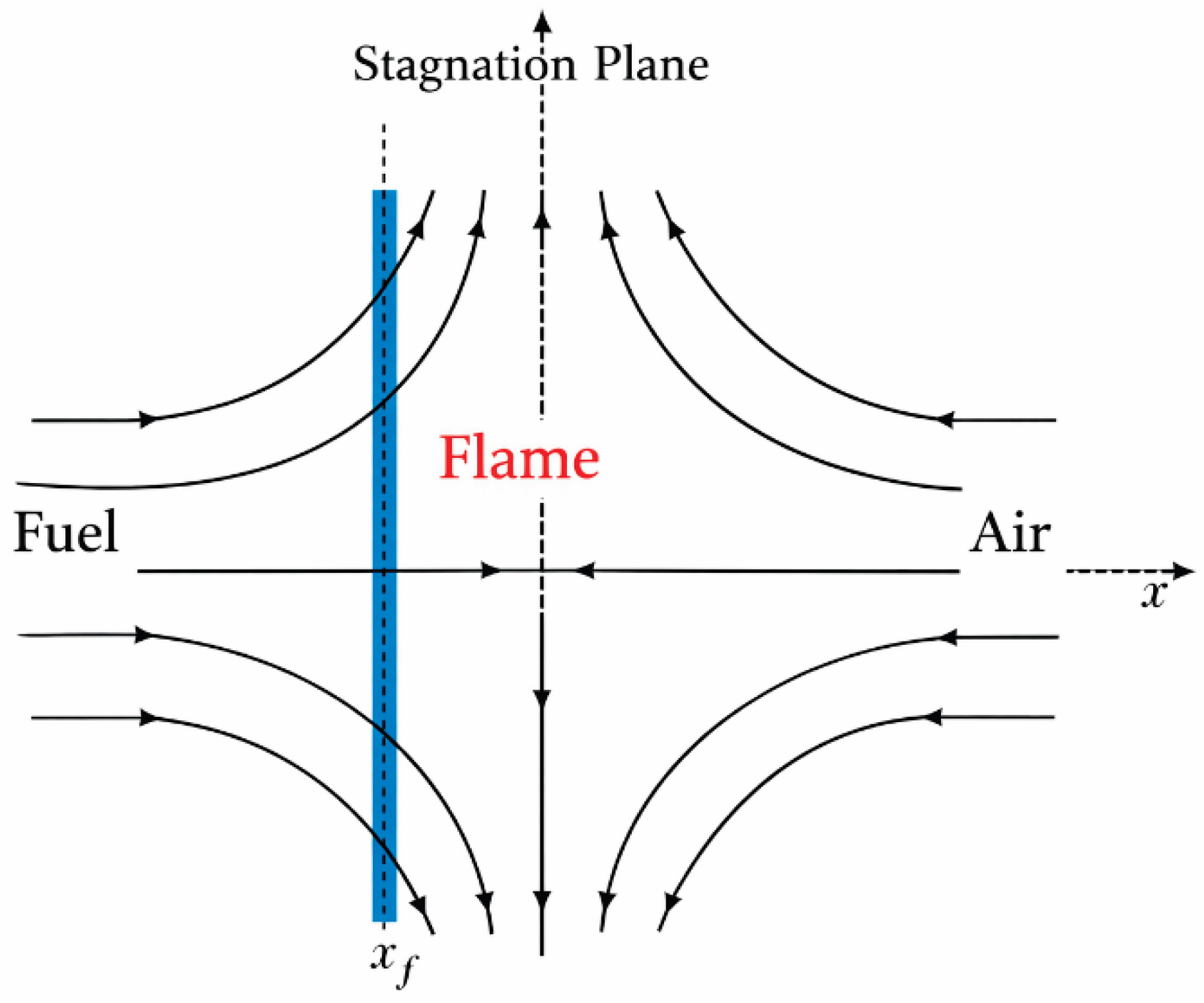
Figure 2.
(a) Schematic representation of the computational domain with the imposed boundary conditions, (b) Grid generation illustrating mesh clustering near the walls using a hyperbolic tangent stretching function.
Figure 2.
(a) Schematic representation of the computational domain with the imposed boundary conditions, (b) Grid generation illustrating mesh clustering near the walls using a hyperbolic tangent stretching function.
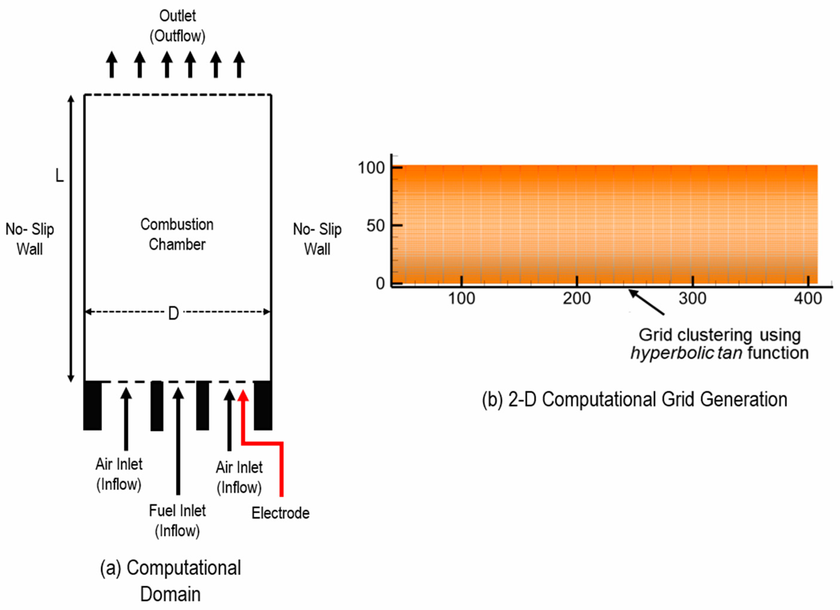
Figure 3.
Comparison of axial temperature distributions for the two-dimensional non-premixed laminar methane–air flame obtained using three different grid resolutions.
Figure 3.
Comparison of axial temperature distributions for the two-dimensional non-premixed laminar methane–air flame obtained using three different grid resolutions.
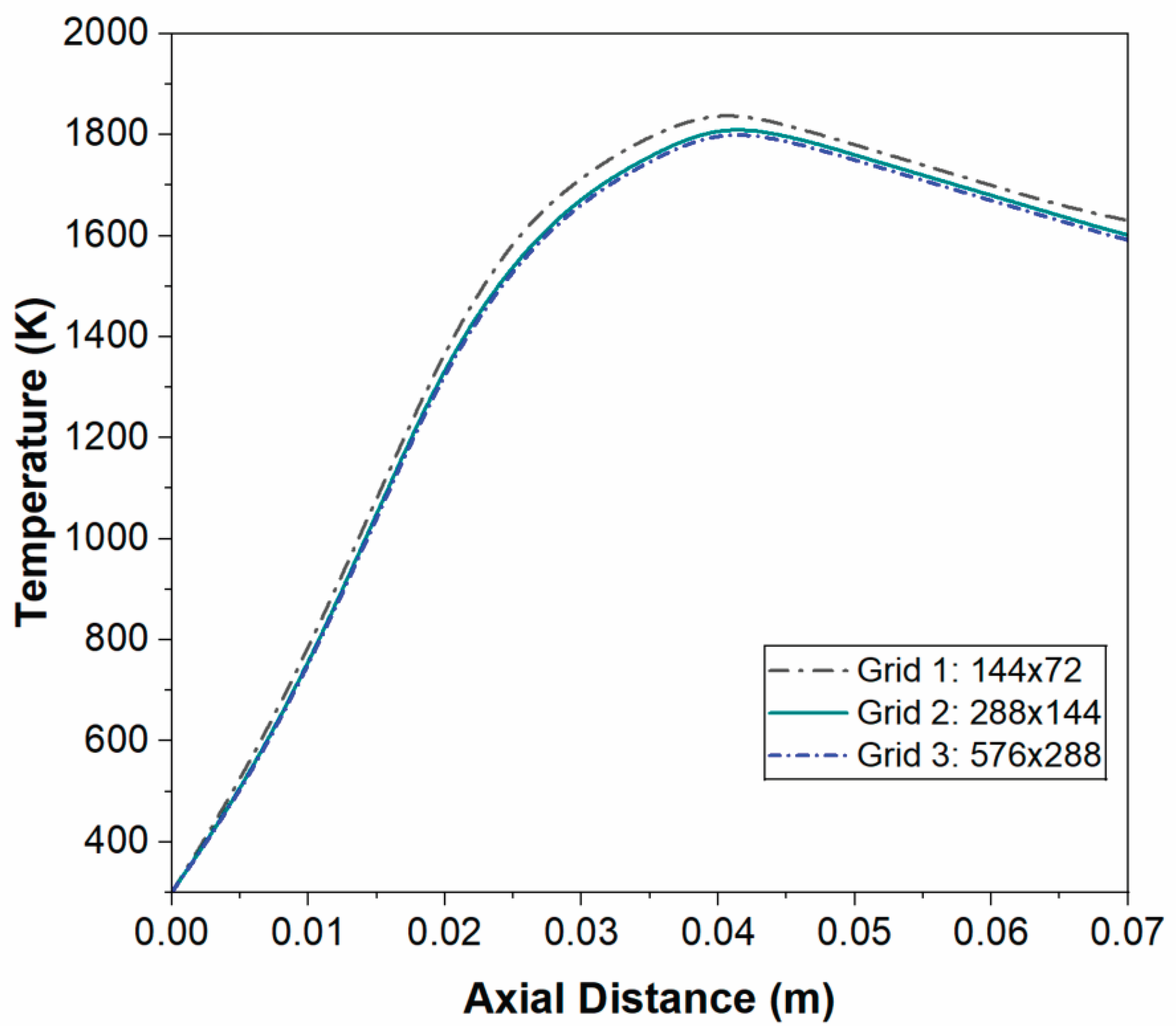
Figure 4.
Temperature–mixture fraction profiles of a laminar methane–air diffusion flame at different axial locations: comparison between the present model and Smooke et al. [43].
Figure 4.
Temperature–mixture fraction profiles of a laminar methane–air diffusion flame at different axial locations: comparison between the present model and Smooke et al. [43].
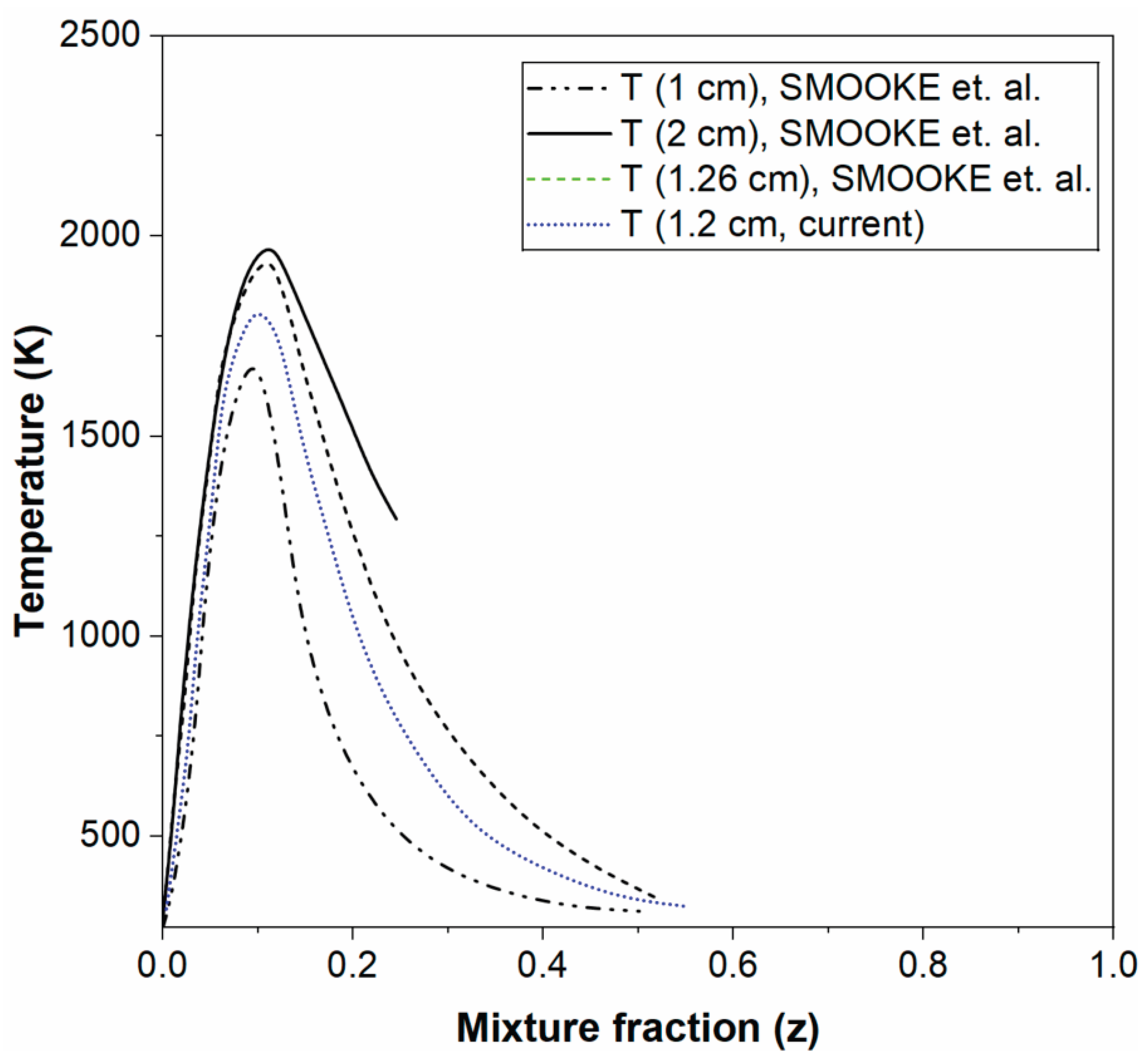
Figure 5.
Contours of OH mass fraction in the r–x plane comparing the baseline case without plasma forcing (left) and the plasma-forced case (right). Plasma forcing significantly modifies the spatial distribution and persistence of OH radicals, indicating enhanced and sustained chemical activity near the jet core and along the axial direction.
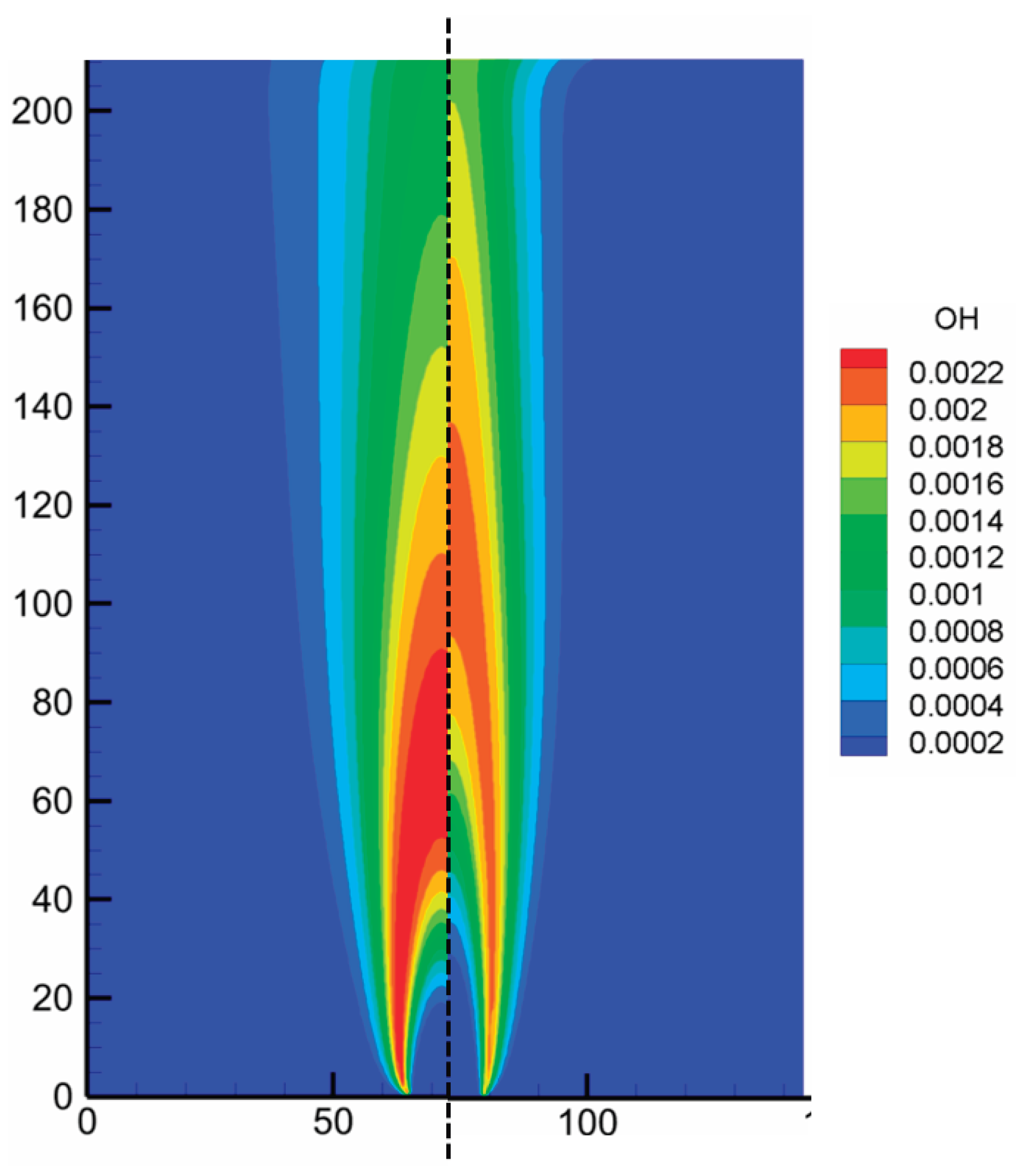
Figure 6.
Contours of temperature in the r–x plane comparing the baseline case without plasma forcing (left) and the plasma-forced case (right). Plasma forcing significantly modifies the spatial distribution and persistence of OH radicals, indicating enhanced and sustained chemical activity near the jet core and along the axial direction.
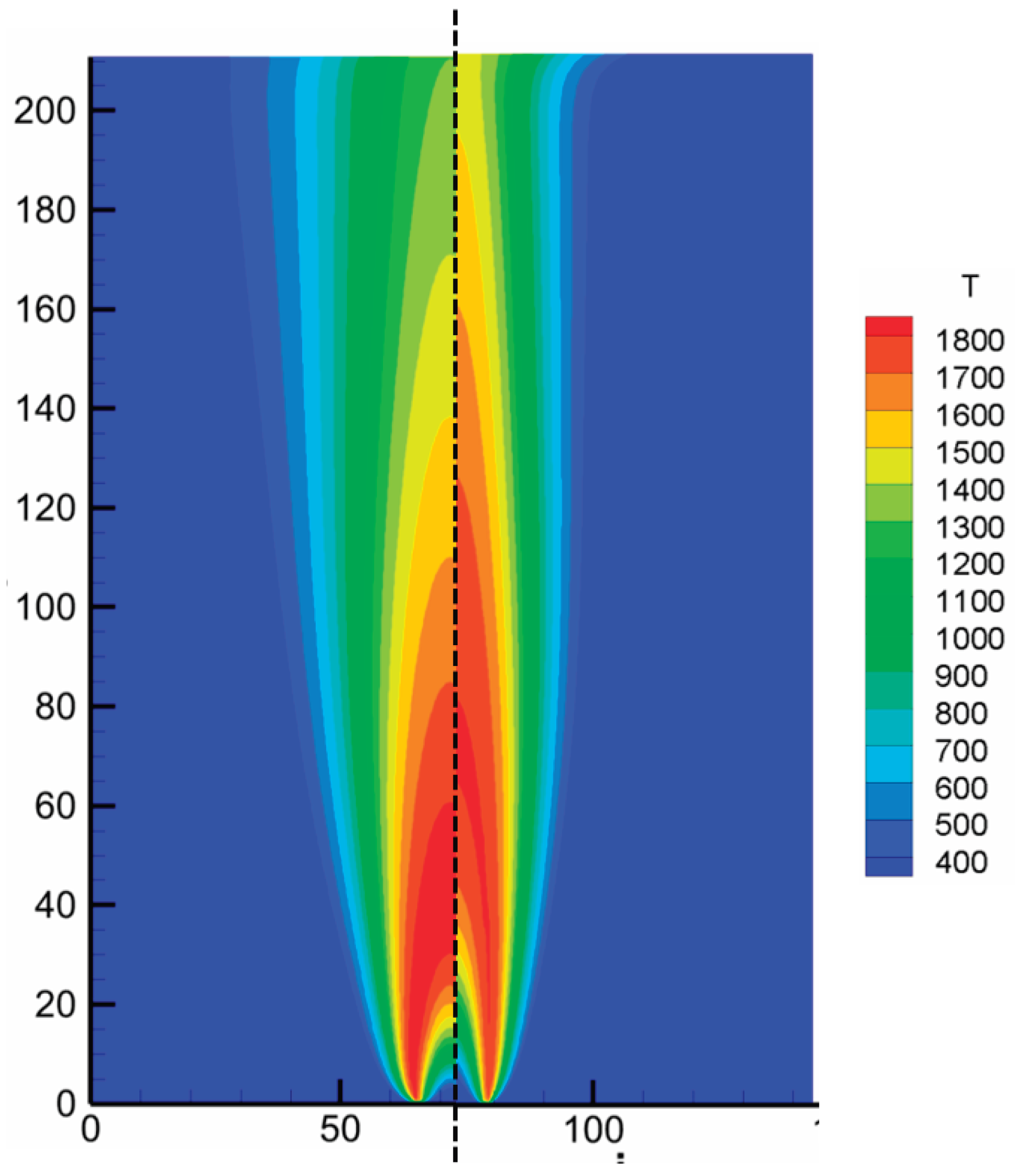
Figure 7.
Contours of temperature in the r–x plane comparing the baseline case without plasma forcing (left) and the plasma-forced case (right). Plasma forcing significantly modifies the spatial distribution and persistence of OH radicals, indicating enhanced and sustained chemical activity near the jet core and along the axial direction.
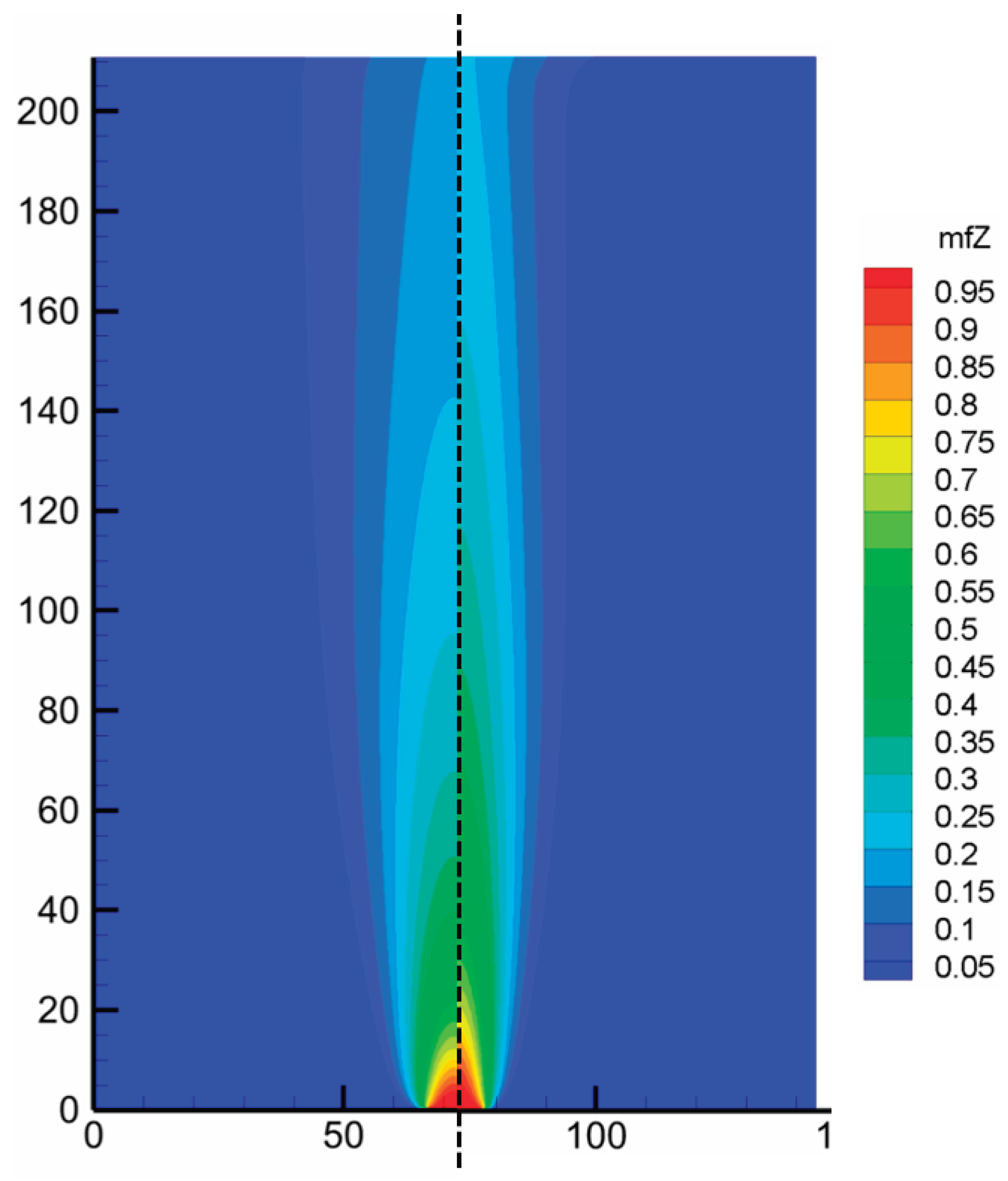
Figure 8.
Contours of temperature in the r–x plane comparing the baseline case without plasma forcing (left) and the plasma-forced case (right). Plasma forcing significantly modifies the spatial distribution and persistence of OH radicals, indicating enhanced and sustained chemical activity near the jet core and along the axial direction.
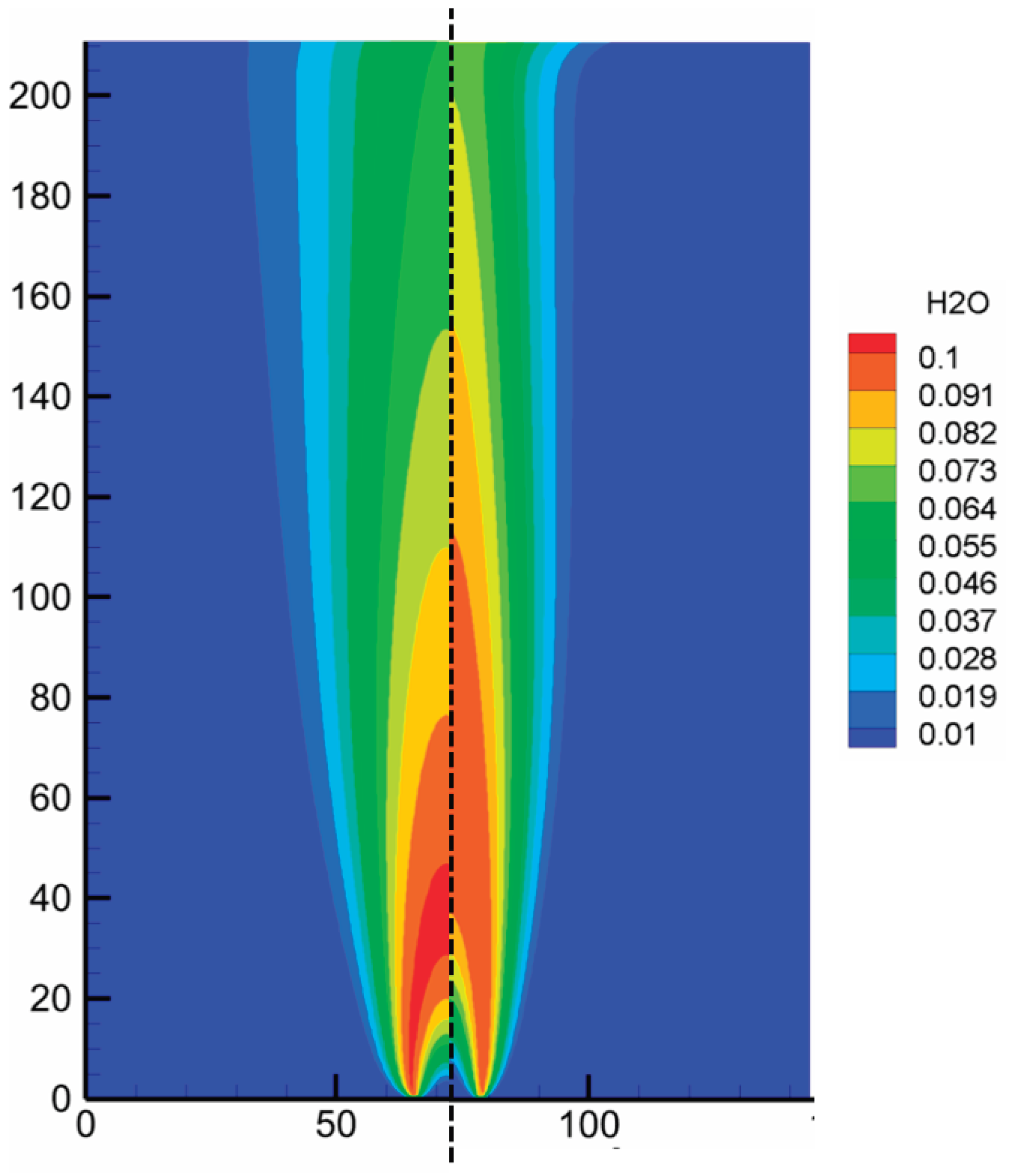
Figure 9.
Radial velocity profiles with and without electric-field forcing at an axial position of 0.5 cm.
Figure 9.
Radial velocity profiles with and without electric-field forcing at an axial position of 0.5 cm.
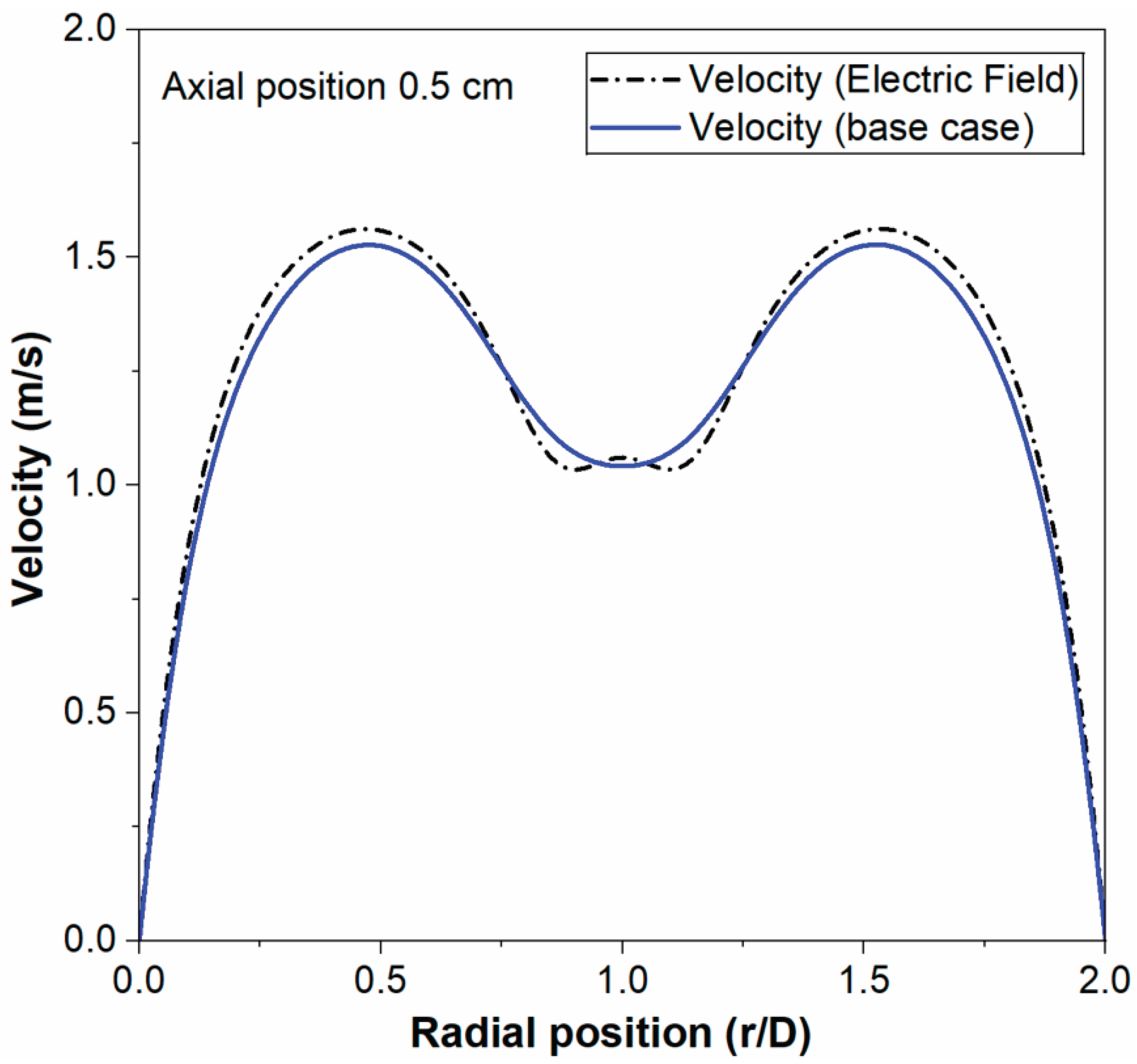
Figure 10.
Radial velocity profiles with and without electric-field forcing at an axial position of 1.8 cm.
Figure 10.
Radial velocity profiles with and without electric-field forcing at an axial position of 1.8 cm.
Disclaimer/Publisher’s Note: The statements, opinions and data contained in all publications are solely those of the individual author(s) and contributor(s) and not of MDPI and/or the editor(s). MDPI and/or the editor(s) disclaim responsibility for any injury to people or property resulting from any ideas, methods, instructions or products referred to in the content. |
© 2026 by the authors. Licensee MDPI, Basel, Switzerland. This article is an open access article distributed under the terms and conditions of the Creative Commons Attribution (CC BY) license.
Copyright: This open access article is published under a Creative Commons CC BY 4.0 license, which permit the free download, distribution, and reuse, provided that the author and preprint are cited in any reuse.


