Submitted:
19 December 2024
Posted:
20 December 2024
You are already at the latest version
Abstract
In the last years the appeal for using methane as green fuel for rocket engines has been on an in-creasing trend due to the more facile storage capability, reduced handling complexity and cost-effectiveness when compared to hydrogen. The present paper presents an attempt to simulate the ignition and propagation of the flame for a 1 kN gaseous methane-oxygen rocket engine using a pintle-type injector. By using advanced numerical simulations, the Eddy Dissipation Concept (EDC) combined with the Partially Stirred Reactor (PaSR) model and the Shielded Detached Eddy Simulation (SDES) were utilized in the complex transient ignition process. The results provide important information regarding the flame propagation and stability, pollutants formation and temperature distribution during the engine start-up, highlighting the uneven mixing regions and thermal load on the injector. This information could further be used for the pintle injector’s geometry optimization by addressing critical design challenges, without employing the need for iterative prototyping during early stages of development.
Keywords:
ignition
; pintle injector
; GCH4/GO2 rocket engine
; EDC
; pollutants formation
1. Introduction
The motivation for this paper came from the need for deeper introspection into the process of combustion and flame propagation inside a rocket engine equipped with a pintle injector. This compelling urge arose when a group of rocketry enthusiasts comprising one of the authors tried to test the ignition of a model thruster which ended up in a catastrophic failure. A posteriori analysis of the remains of the engine showed that the ceramic insulator of a misplaced spark generator detached and impacted the throat of the nozzle leading to failure.
The designed engine was designed to produce 1k N of thrust, at sea level, with a specific impulse of 273 seconds, at a chamber pressure of 20 bar and 0.435 kg/s total mass flow rate. The oxygen-fuel mixture ratio used was 3.6.

Table 1.
Engine parameters.
| Parameter | Values at sea level |
|---|---|
| Thrust (N) | 1000 |
| Chamber pressure (MPa) | 2 |
| O/F ratio | 3.6 |
| Oxidizer injection temperature (K) | 300 |
| Fuel injection temperature (K) | 450 |
| Specific impulse (s) | 273 |
| Total mass flow rate (kg/s) | 0.435 |
The only parameter measured from the experiment was the thrust, of 950 N. This same engine is part of another work by the same authors [1], aiming to provide a water-based active cooling system, on a reduced-scale engine.
Figure 1.
Experimental test conducted on the first iteration of the 1 kN gaseous engine.
This new experimental engine (Figure 2.), has an improved injection system, comprised of a redesigned static pintle injector, a new location for a high temperature custom-made spark generator, in the upper recirculation zone, providing a constant flux of cold gasses to the igniter, as well as the active water-based cooling system mentioned above.
Apart from previous research [1] that dealt with steady joint combustion and cooling of the thruster, our present investigation aims to discover insights into the ignition process and flame front propagation at engine start-up. The pintle injectors are recognized for their effectiveness in propellant mixing and ability to deeply control the throttle of a liquid rocket engine. During the years of their usage, there have been no records indicating any combustion instability, moreover their simple design, of only two main elements, along with the advancement of 3D Additive Manufacturing technologies, enabled a more economical approach to the iterative process of liquid rocket engine injector development. The main components of a pintle injector are the central element with a pintle tip, providing radial flow for one of the propellants and a circumferential annulus, providing axial flow for the other propellant, thus, the two species intersect each other in an impingement point. The exceptional combustion efficiency and the deep throttling ability, even with 250:1 chamber pressure and 50000:1 thrust scaling, with 25 different propellants [2], provides the pintle injector with functional advantages over other types of injectors.
2. Literature Review
The reason for which the combustion simulations on engines with pintle injectors is crucial is related to the pintle tip exposure temperature, which could create permanent damage in a very short time. The ablation of the pintle tip could create a catastrophic failure, such as presented by the work of Yibing Chang and Jianjun Zou [3] studying the ablation suffered by a 500 N gaseous engine using a pintle device. In this work, the stainless steel pintle tip suffered extreme ablation due to the chromium precipitates at temperatures over 1273 K. The study was performed on 3 different O/F mixture fractions: 0.8, 2 and the designed operation condition fraction of 3.2. The numerical simulation was performed using a reduced six-step Jones-Lindstedt mechanism [4], the k – ε turbulence model and ideal gas density properties, with the thermal conductivity of the pintle tip set to 18.3 W/(m ∙ K). The comparison between the numerical approach and the experimental results showed that a preliminary analysis regarding the thermal load and combustion flow can be used, until a higher fidelity model is developed.
The paper written by V.M. Zubanov et al [5], presents a method for simulating transient combustion in a rocket engine that uses gaseous hydrogen and oxygen. In this paper, three simulation models were studied: Eddy Dissipation Model (EDM), Finite Rate Chemistry (FRC), and Flamelet combustion model. The results showed that the EDM model can produce quick and qualitative results, although the temperatures obtained from this approach are excessive.
Another issue with using the EDM model in non-stationary simulations is that it does not account for the reaction rates of systems containing multiple reaction steps, meaning the model can only be successfully used for reactions that have two steps. Therefore, the FRC combustion model was addressed, which uses the Arrhenius equation to determine the reaction rate. However, this approach was also unsuccessful. One probable reason for the simulation’s volatility was the lack of consistency among the reaction rates, which varied from one reference to another one. After implementing reaction models from the work of Gerasimov et al [6], which provides 26 reaction equations, the stability of combustion still could not be achieved by the authors. The next step was implementing the Flamelet model [7,8]. Using this approach, the authors obtained satisfactory results, solving the problem created by the EDM model, which overestimated the temperature in the combustion chamber. In this model, combustion occurs at the fuel-oxidant mixture front, with a low reaction time given the presence of unreacted components as noticed by the authors.
A chemical equilibrium model for a 3D analysis on a liquid propellant rocket engine with a pintle injector was implemented by Youngsung Ko et al [9] covering the combustion performance and the efficiency of pintle tip cooling. The coupled pressure-based transient simulation was performed using the SRK real gas density model with the k – ε turbulence model. The chosen method provided similar results to the experimental campaign regarding the temperature distribution on the tip of the pintle injector, even though the chemical equilibrium model overestimated the overall combustion temperature.
In liquid-gas combustion modeling withing Liquid Rocket Engines, the implementation of the Discrete Phase Modeling in combination with a species transport model, such as FRC, EDM, FRC-EDM hybrid, or the EDC model, enables a complex analysis of the atomization and combustion characteristics of the injector. These include the skip distance in pintle injectors, documented in Fang’s work [10]. The study, performed with a single-step reaction mechanism and the EDM transport model, showed that a ratio of 1 between the total length of the pintle in the chamber and its diameter provides the maximum combustion efficiency.
A study covering the formation of a new recirculation zone when a center post radius Is implemented into the pintle injector design [11], provided a method of combustion simulation based on the EDC model, calculating the reaction rates using small-scale eddies generated by turbulent kinetic energy and turbulent dissipation. This approach, combined with a reduced Jones-Lindstedt 6-step mechanism [12] can provide more accurate predictions regarding the flame length and temperature when compared to the PDF approach [13].
The Flamelet Generated Manifold (FGM) methodology, developed by Oijen and de Goey [14], which implements the flamelet model, can consider the transport effects while also reducing the computational time and decrease enthalpy value error to 0.1%, when compared to the ILDM error of 9% [15]. This concept was applied in combustion simulations with swirl injectors, with the paper by A.V. Brito et al [15], showing that the mixture fraction flame using a URANS-non-adiabatic-FGM is more accurately predicted than the published LES model results. The application of the FGM model for the non-premixed and partially premixed flows shows that for a forced ignition, the local temperature can exceed the adiabatic flame temperature, due to the preheated vapor, observed in a spray ignition simulation. The FGM approach is mostly used for gas-liquid combustion, under supercritical conditions [16].
The current research regarding ignition and flame propagation in engines with pintle injectors is quite scarce. To the best of our knowledge, there are only a handful of papers in the open literature on this subject. The most comprehensive study [17] discusses the start-up process for a model LOX/GCH4 engine describing, mainly from an experimental point of view, the spraying and mixing stage as well as the torch ignition and flame anchoring around the pintle tip. The simulation was only related to LOX spray development.
Acknowledging the lack of expensive and cutting-edge technology to set up an experimental test bench, our current endeavor is focused only on spark ignition simulation and further flame development for GOX/GCH4 combustion chamber with a pintle injector of our own design.
3. Numerical Methodology
3.1. Shielded Detached Eddy Simulation (SDES) Model
This model is an advanced hybrid RANS-LES approach for turbulent flows designed for wall bounded flows with high Reynolds numbers. The SDES model [18] (p. 111) is based on the Delayed Detached Eddy Simulation (DDES) framework [19] (p. 1006), handling turbulent flows by using both the RANS approach, at the boundary layer regions, and the LES approach for the detached flows.
The RANS model used for the SDES turbulence model is the Shear Stress Transport SST (k-ω), governed by the following transport equations:
and
in which is density, is the turbulent kinetic energy, is the specific dissipation rate is the turbulence kinetic energy generation, is the generation of , and are the effective diffusivity of and , and are the dissipation due to turbulence of and , and are source terms defined by the user and the buoyancy terms are accounted for by and .
The first step in obtaining SDES starts with the DDES-SST model, in which the dissipation of the turbulent kinetic energy is modified for the DES model:
in which is a model constant, and is:
The SDES introduces a shielding function preventing premature LES switching at the RANS boundary layer, while also improving the grid length scale definition for a smoother RANS to LES transition. The SDES formulation in two-equation models is attained by modifying the sink term in the equation. For SST, the modification brings the addition of a dissipation rate term defined below:
where is the specific SDES blending function:
is the turbulent length scale, is a calibration parameter for the RANS to LES transition, is a blending function controlling how much of the flow is treated as RANS and how much as LES, it has a range between 0 and 1. When the value is 1 the model is using RANS, while at a value of 0 it behaves like LES. determines the blending level between RANS and LES, assuring that the switch is not made to LES if it not appropriate. is the mesh length scale for the SDES model:
in which is the control volume in the mesh cell and is the maximum grid spacing.
3.2. Eddy Dissipation Concept (EDC)
The nature of the simulation implies a transient formulation during the ignition process consisting of running the whole simulation as time dependent, method which also provides a more precise visualization of the injection flow, as well as a more precise timing for the ignition, preventing detonation. The combustion process generated with the pintle injector can be very well circumscribed in the partially premixed combustion environments which represents a combination between non-premixed (diffusion) and premixed combustion systems. The non-premixed combustion occurs, primarily, near the pintle tip, where the mix of the fuel and oxidizer is predominantly done by turbulent diffusion, while the premixed combustion is mostly developed downstream in regions where the recirculation zones and turbulence promote a more complete mixing of the reactants, thus creating a hybrid flame structure.
The species transport Is governed by the following conservation equation [18] (p. 222):
Herein, is the mass diffusion, is the mass fraction of the species, is the velocity of the fluid flow and is the source term. For turbulent flows, the mass diffusion is computed by Ansys Fluent in the following way [18] (p.222):
in which is the species mass diffusion coefficient for in the mixture, is the turbulent viscosity, is the thermal diffusion coefficient, is the local mass fraction of the species and is the turbulent Schmidt number (0.7 in this case).
As an extension to the Eddy Dissipation Model (EDM), EDC also includes the finite-rate chemical reactions by accounting a slower reaction time than the one given by turbulent mixing, while EDM assumes that the chemical reaction is instantaneous. The EDC model calculates the reaction rates in the small-scale eddies accounting for the eddy residence time. While EDM calculates the reaction rate by comparing the availability of reactants and the turbulent dissipation rate and using whichever is lower from the two, EDC defines the source term as follows:
where denotes the species mass fraction at the finite scale after undergoing reactions over the time scale . The molar rate of creation or destruction of species in the rth reaction of the chemical mechanism following Arrhenius form is expressed as
Here, is the net effect of third bodies on the reaction rate, is the molar concentration of species, is rate exponent for reactant species in reaction , is the rate exponent for product species, is the forward rate constant, is the backward rate constant, with and being the stoichiometric coefficients for reactant and, subsequently, product.
Since in the standard EDC model the length scale constant and the time scale constant do not depend on the chemistry variables or local flow, in certain conditions in which slow chemistry is taking place due to strong oxygen dilution the model greatly overestimates the temperature magnitudes [16]. Attempting to fix this overestimation, a combination of the EDC model with the partially Stirred Reactor (PaSR) has been studied in several papers, being applied to both supersonic and mild combustions [20, 21]. This approach differs from the standard EDC model by an alternative definition of the time scale and reacting volume fraction:
where is the Damköhler number:
Ansys Fluent computes the chemical time scale based on the reaction rates of , , , and
while the mixing time scale is expressed as a fraction of the turbulence integral time scale , where is a function of the local turbulent Reynolds number.
The mechanism used is the detailed GRI-Mech 3.0 [22], developed mostly for the combustion of hydrocarbon fuels, primarily for methane, providing great insight regarding the formation of pollutants and flame behavior due to the inclusion of the important , , and radicals. Even if the main application for GRI-Mech 3.0 remains the methane-air combustion, the incorporation of reburn chemistry and NO formation provides important evaluation of pollutant formation during start-up, emphasizing the need to develop environmentally sustainable propulsion systems. Even if skeletal mechanisms are more computationally efficient and potentially more suitable for methane-oxygen combustion, the transient ignition process could benefit more by the GRI-Mech 3.0 detailed chemical pathway by noticing that the ignition process in atmospheric conditions takes places in the presence of nitrogen, which most skeletal mechanisms do not use. A comparison and trade-off analysis between the skeletal mechanism and the current mechanism, regarding the accuracy and computational cost, could be explored in future work.
3.3. Peng-Robinson Real Gas Model
As the pressure in the combustion chamber increases during the ignition process, the properties of the gases start to deviate from the ideal gas behavior, experiencing non-ideal compressibility. For this reason, a real gas model, using cubic equations of state (EOS) like Peng-Robinson, could better predict the enthalpy, entropy and density of the products, leading to a more accurate representation of the flame propagation. The Peng-Robinson real gas model uses the same general cubic equation of state employed by most of the other models:
In which is the absolute pressure, is the specific molar volume, is the temperature, is the universal gas constant and the , , , and are coefficients given for each equation. In the Peng-Robinson model, , and . The three necessary parameters required for using the model are the critical temperature , the critical pressure and the acentric factor . In this case, as the Peng-Robinson cubic equation of state is used, the specific coefficients are defined, using the three required parameters, as follows:
where the temperature dependence of is given by the following function, also used in the Soave-Redlich-Kwong Equation:
in which , specific to the Peng-Robinson EOS, is:
3.4. Spark Model
Spark ignition represents a very complex phenomenon involving plasma kinetics, fluid dynamics, chemical kinetics, and molecular transport. It also poses a lot of mathematical difficulties due to the stiff nature of all these processes. The spark model works by introducing a localized heat source in a user-defined location and converting instantaneously, within a limited number of cells, the unburned reactants into combustion products. The species composition and the temperature are calculated every time-step by using the equilibrium burn composition and the unburned composition :
The radius of the spark increases in time according to [17] (p. 396):
in which is the density of the unburned fluid ahead of the flame front, is the density of the burnt fluid behind of the flame, and is the turbulent flame speed. In this paper, the Turbulent Length model was chosen, ignoring the flame curvature effects applied to the flame speed, thus:
Where is the spark radius at the given moment. The spark sphere radius is calculated as follows:
This equation is used to ensure that the volume of the sphere is not too large or too small relative to the cell size. Here, is the initial spark radius, defined by the user, is the cell length scale and is the turbulent length scale. When the dimension of the spark reaches the turbulent length scale, Ansys Fluent switches off the spark flame model and it is replaced by the selected model in the species settings, governed by the Zimont model [23] (p. 1035), [24] (p. 1035), [25] (p. 1036), based on the assumption that equilibrium small-scale turbulence exists in the laminar flame, leading to a turbulent flame speed expression written using only large-scale turbulent parameters:
in which is the model constant, is the RMS velocity, is the unburnt thermal diffusivity, is the turbulence tie scale and is the chemical time scale. This is applicable when the Kolmogorov scale is smaller than the flame thickness and penetrates in the flame, defined as the reaction zone combustion zone, determined by Karlovitz number:
where is the characteristic flame scale, is the Kolmogorov turbulence time scale and is the Kolmogorov velocity.
4. Computational Approach
A wedge axisymmetric configuration of the combustion chamber presented in Figure 2 and connected with an ambient control volume is illustrated in Figure 3. This is the computational domain subject to our analysis. The domain was meshed with different resolutions following a quadrilateral dominant strategy to obtain an almost complete rectangular grid which is depicted in Figs. 4a and 4b. Due to the very fine grid size, only the most relevant details have been presented reflecting the rectangular shape and inflation layers near the walls.
Given the limitations of computational resources, a grid independence test has been performed only for steady combustion simulation. Element sizes ranging from 0.3 to 0.12 mm have been used to obtain grids only in the combustion chamber counting from 100000 to 400000 elements. Additionally, starting with the 100000 cells grid, automatic refinement strategy has been developed with two different features. For mesh denoted Adapt 1, the refinement was done with a higher frequency leading to a grid counting around 300000 elements, while for the one denoted Adapt 2 the frequency was half the frequency of Adapt 1, thus obtaining a grid of around 200000 cells. The most important parameters have been compared among Adapt 1, Adapt 2 and a 400000 elements rectangular grid. The results presented in Figure 5 along a vertical probe line situated 6 mm downstream of the pintle outer wall show a very good correlation among the three grids. Given the highly unsteadiness of the flow during the ignition process, a grid refining procedure, although possible, would be very computationally expensive. Hence, it was decided to work on the 400000 elements rectangular grid inside combustion chamber. The overall structured mesh contains 793879 cells.
Figure 4.
Mesh structure at: a) the injector region and b) the chamber upper-left corner.
The simulation was computed using an adaptive time-step transient approach with pressure-based solver and unity Courant number, and Prandtl number equal to 0.85. For the boundary conditions, the mass flow inlet condition was chosen for both the reactants, 0.09475 kg/s for methane, at a temperature of 450 K and 0.34043 kg/s for oxygen at 300 K.
Figure 5.
a) Temperature distribution b) Absolute pressure distribution.
The outlet region is set as a pressure outlet at 0 Pa gauge pressure, at 300 K, with the backflow species being 76.6% nitrogen and 23.4% oxygen, while the Air inlets are pressure inlets with a gauge pressure equal to 0 and the same backflow settings as the pressure outlet. All domains were initialized at an operating pressure equal to the atmospheric pressure, with 23.4% oxygen and 76.6% nitrogen, at a temperature of 300 K. Adiabatic conditions have been set for all solid walls. For this research, no radiation has been accounted for. Regarding the material properties, the laminar flame speed needed to compute the spark evolution was chosen as a constant with a value of 0.4 m/s. It is acknowledged that a constant value for the laminar flame is debatable, but the current EDC implementation makes difficult the introduction of the laminar flame speed dependence on unburnt mixture temperature, pressure and equivalence ratio. Anyway, recent investigations on CH4/O2 mixtures are still not able to produce reliable values for the laminar flame speed at high pressures for rocket engines applications [26].
The spark igniter is located at 11 mm from the vertical chamber wall and 26 mm from the symmetry axis. The spark adds no energy into the flow. The thermo-chemical state behind the spark flame front is instantaneously equilibrated as the spark propagates, and the burnt temperature is the equilibrium temperature [18] (p. 396). A cold flow was run for 1 millisecond to allow a small fraction of fuel and oxidizer to enter the chamber, so detonation can be prevented during the ignition. After the 1 millisecond cold flow time, the spark was initialized and ran for 0.5 millisecond.
5. Results
The results presented below (Figure 6, Figure 7, Figure 8, Figure 9, Figure 10, Figure 11, Figure 12, Figure 13, Figure 14, Figure 15 and Figure 16) are related to the time flowing from the moment of ignition. The flame front velocity can be estimated based on the propagation between the ignition starting time (Figure 6a) and 0.1 milliseconds after it by measuring the distance which the flame traveled during this time. The flame propagated 0.01853 m (18.53 mm) in 0.1 milliseconds (Figure 6b), resulting in a flame front speed of 185.3 meters per second, during the ignition, for a gauge pressure of 0 Pa and a still consistent amount of air inside the chamber. In this way, the choice of 0.4 m/s option for the laminar flame speed can be explained. The turbulent flame speed obtained is consistent with values obtained in similar simulations using FGM model. Efficient ignition is indicated by the rapid rise in temperature, due to the pintle injector mixing properties.
During the first instances of the ignition process, the flame front is advected along the spray cone (Figure 6b), then it spreads on the upper wall forward and backward (Figure 6c). The main vortex downstream of the pintle produces bending of the flame front and burnt gases starts approaching the injector to sustain combustion (Figure 6d). It has been remarked that all along the spark duration the instantaneous maximum value for temperature overshoots the adiabatic flame temperature (~ 3440 K). This effect is the consequence of the temperature conditions behind the spark introduced by turbulent flame velocity (Eq. 25 or 26) that modifies the source term in the energy equation. Once the spark is switched off, the maximum temperature does not go beyond the adiabatic temperature. The instantaneous evolution of various field distributions for temperature, velocity and the main species of interest , , , , and are depicted in the following snapshots for two different time stamps, 1ms and 6ms from the initiation of the spark.
Figure 7.
Instantaneous temperature distribution. a) 1 millisecond; b) 6 milliseconds.
According to Figure 6 and Figure 7 it can be stated that the location of the spark very close to mixture spraying cone is beneficial and works to create a stable combustion zone, an efficient flame propagation, leading to a continuous combustion. The temperature stabilization downstream (Figure 7b) indicates that the flame is fully developed. Within the given assumptions, we notice a consistent thermal load exerted on the outer wall of the pintle.
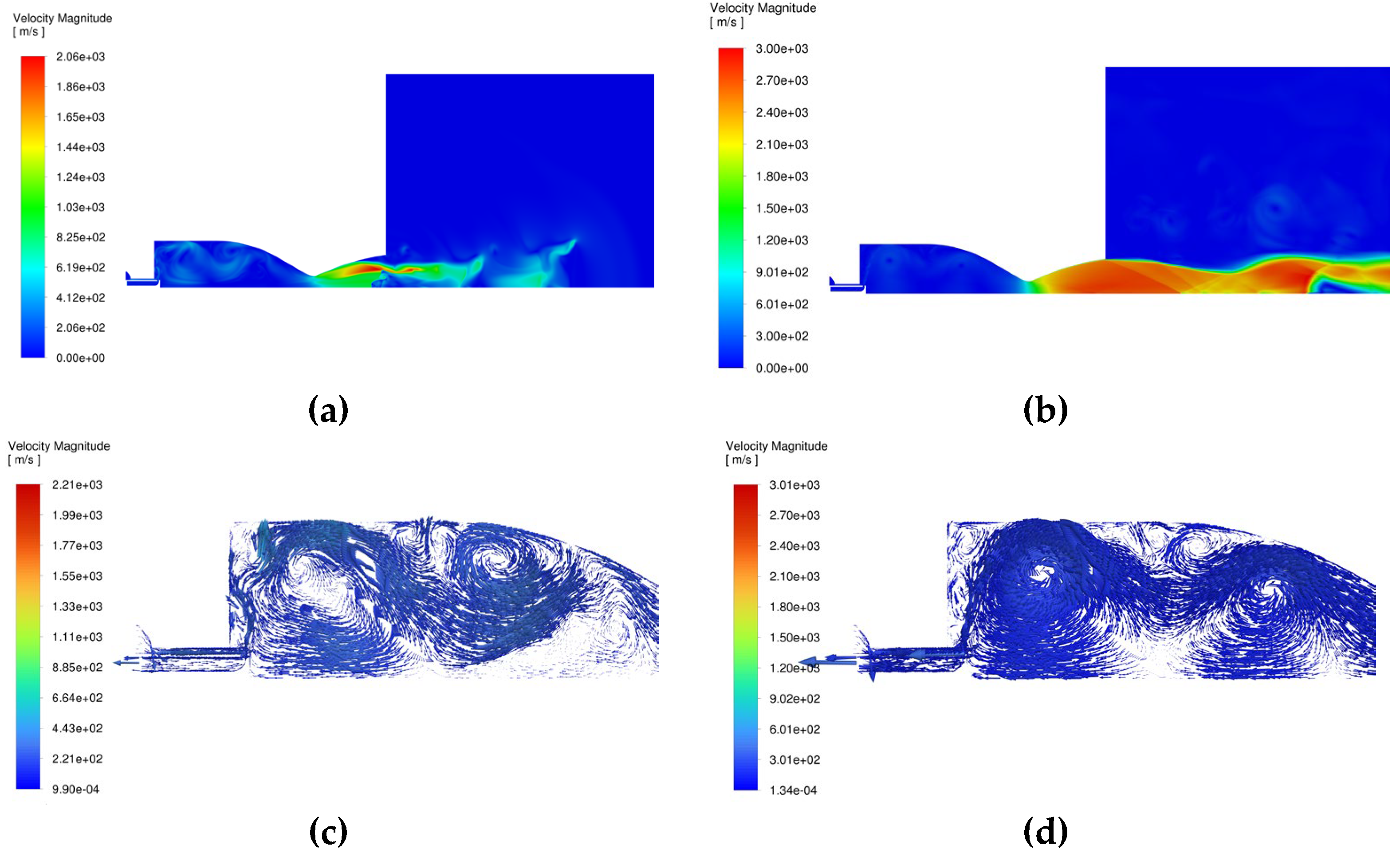
Figure 8.
Instantaneous velocity magnitude distribution. a) 1 millisecond; b) 6 milliseconds; c) velocity vectors at 1 millisecond; d) velocity vectors at 6 milliseconds.
Figure 8.
Instantaneous velocity magnitude distribution. a) 1 millisecond; b) 6 milliseconds; c) velocity vectors at 1 millisecond; d) velocity vectors at 6 milliseconds.
The recirculation zones are produced during the first milliseconds of the flow (Figure 8c and Figure 8d), increasing the flame stability by extending the residence time and increasing the thorough mixing of the reactants. The results obtained show that these zones improve the fuel-oxidizer reaction, actively producing a stable combustion process. The mixing of the reactants is promoted by the widespread range of gas flow speeds inside the turbulent recirculation zone.
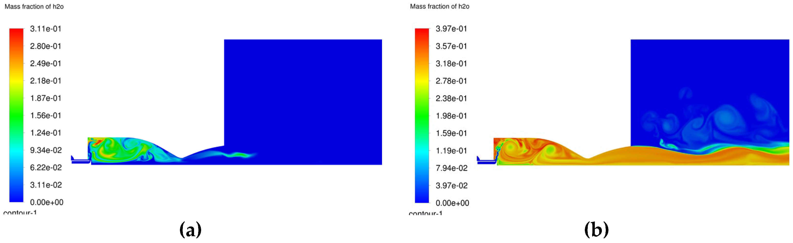
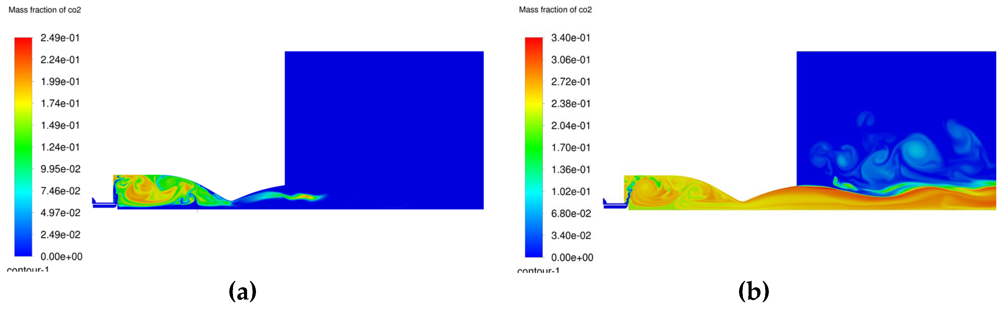
Figure 9.
Instantaneous water vapor distribution. a) 1 millisecond; b) 6 milliseconds.
Figure 10.
Instantaneous carbon dioxide distribution. a) 1 millisecond; b) 6 milliseconds.
It can be observed that during the first time steps of the ignition process, both the carbon dioxide and water vapor are retained inside the chamber due to the developed recirculation zones. Once the temperature and pressure increase, the products are accelerated through the nozzle. Recirculation of these products for a certain time inside the chamber can lead to maximizing the combustion efficiency.
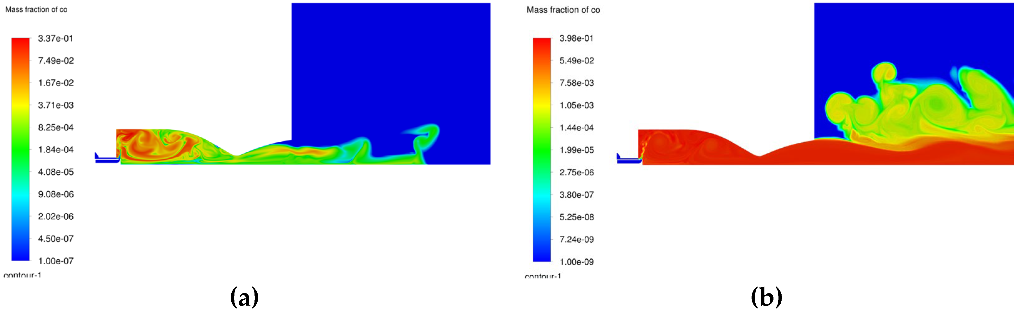
Figure 11.
Instantaneous carbon monoxide distribution (Logarithmic scale). a) 1 millisecond; b) 6 milliseconds.
Figure 11.
Instantaneous carbon monoxide distribution (Logarithmic scale). a) 1 millisecond; b) 6 milliseconds.
The highest rate of carbon monoxide production mostly occurs near the mixture spraying cone (Figure 11a-b) due to incomplete carbon oxidation because of relatively low local temperature concurrent with uneven mixing. Once CO is recirculated to higher temperature zones it will be converted to CO2. As can be seen from Fig. 11b this is a slow process taking more time than the time for convection through the nozzle and downstream outside in the environment. It also shows that the recirculation zones do not sufficiently increase the residence time for CO/CO2 conversion. The slowing down of the CO/CO2 conversion is more pronounced as the burnt gases are cooling down after passing the throat of the nozzle. Obviously, this represents a loss of available energy, loss of combustion efficiency and maybe a further objective for combustion chamber and pintle optimization.
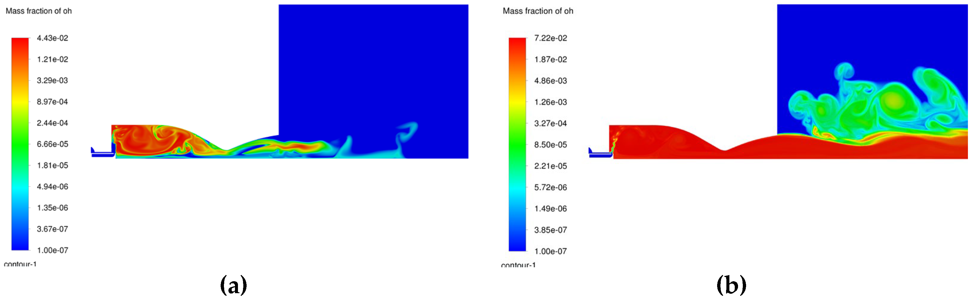
Figure 12.
Instantaneous hydroxyl radical distribution (Logarithmic scale). a) 1 millisecond; b) 6 milliseconds.
Figure 12.
Instantaneous hydroxyl radical distribution (Logarithmic scale). a) 1 millisecond; b) 6 milliseconds.
The fast hydroxyl radical production follows the areas of high reaction rates, where higher temperatures accelerate its formation. This also shows a well-sustained flame, enhanced by the pintle’s injector promotion of the flame propagation through radical generation. Part of the OH is convected through the nozzle and starts depleting mostly due to temperature drop leading to reaction mechanism termination.
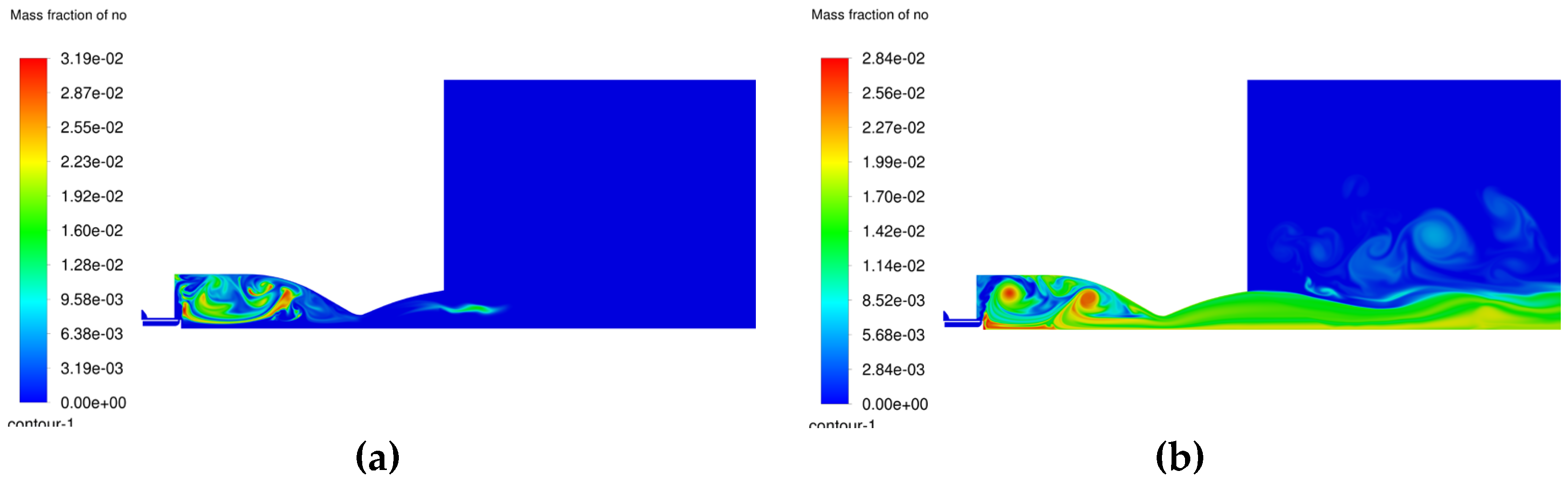
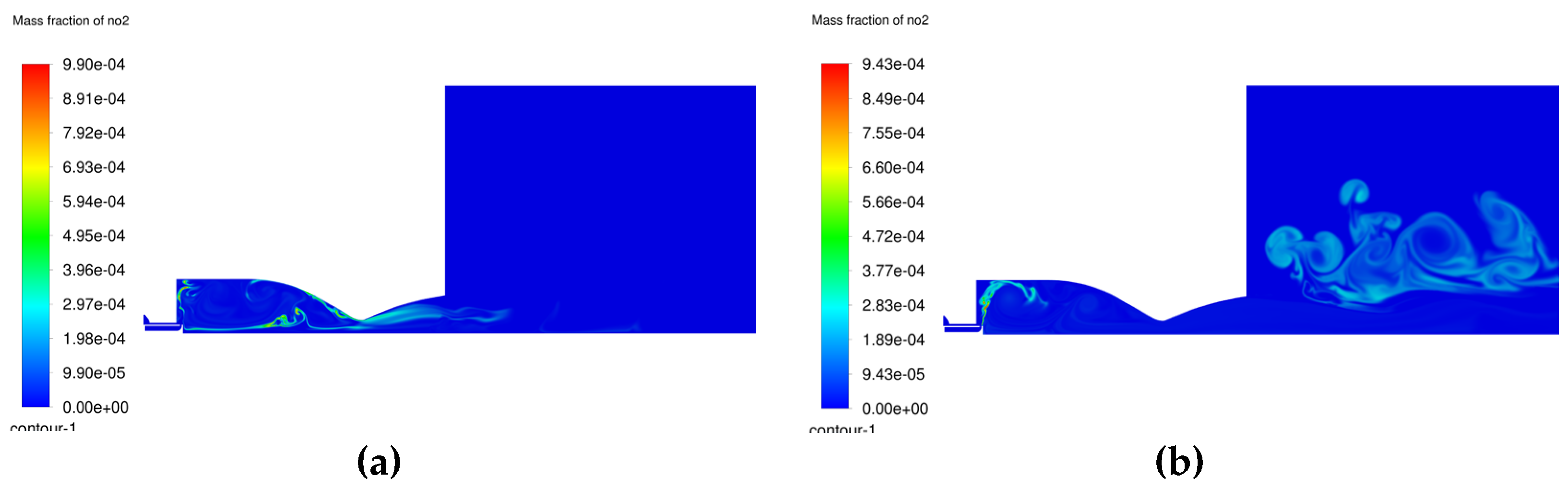
Figure 13.
Nitric oxide distribution. a) 1 millisecond; b) 6 milliseconds.
Figure 14.
Instantaneous nitrogen dioxide distribution. a) 1 millisecond; b) 6 milliseconds.
The growing concern regarding the environmental impact of pollutants also concerns the development of space propulsion, with international emphasis increasing on green propulsion systems. Thus, an analysis was performed on the NOx production inside the chamber, since the presence of these products is a consequence of nitrogen presence in the initial stage of ignition in the chamber. Even if the flow of the fuel-oxidizer mixture will push most of the initial air outside the chamber, there will still be a sensible amount of air trapped inside chamber at the inception of combustion. The nitric oxide distribution looks very similar to the hydroxyl radical distribution, at least in the first millisecond from ignition (Figure 13a). Then, once the temperature has settled, the flame inside the chamber will continue to produce nitric oxide until the exhaustion of nitrogen. Contrary to the distribution of NO, the production of NO2 resides mostly outside the combustion chamber, where nitric oxide reacts with the oxygen present in the atmosphere, suggesting that it is mostly an external effect (Figure 14b).
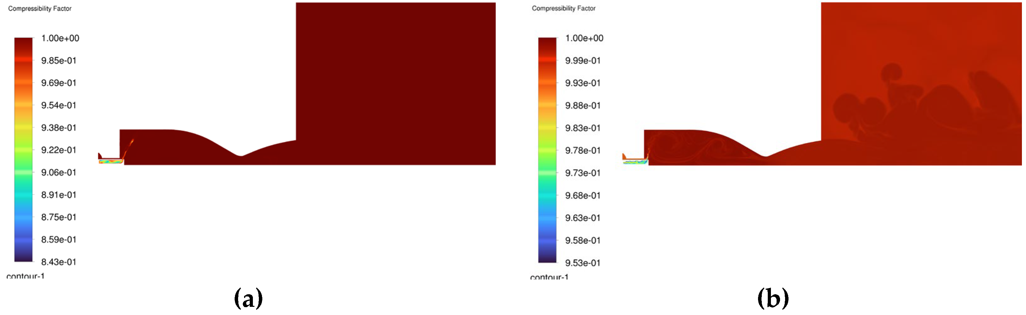
Figure 15.
Compressibility factor. a) 1 millisecond before ignition; b) 6 milliseconds.
The picture above shows the change in the compressibility factor distribution inside the combustion chamber at two different flow times, 1 millisecond before the ignition and 6 milliseconds after the ignition. The zones in which the compressibility factor is below unity represent areas where gases depart from the ideal gas model. This is mostly visible in Figure 15 a), before ignition, near the mixing cone and injector, where the compressibility factor is well below 1, suggesting increased intermolecular forces. -Conversely, in Figure 15 b), the compressibility factor is close to 1 in most regions where temperature has increased substantially due to the combustion process. Still, deviations are persisting in areas with intense turbulent mixing. Thus, the use of real gas models, such as the Peng-Robinson EOS, plays a significant role in determining injector performances.
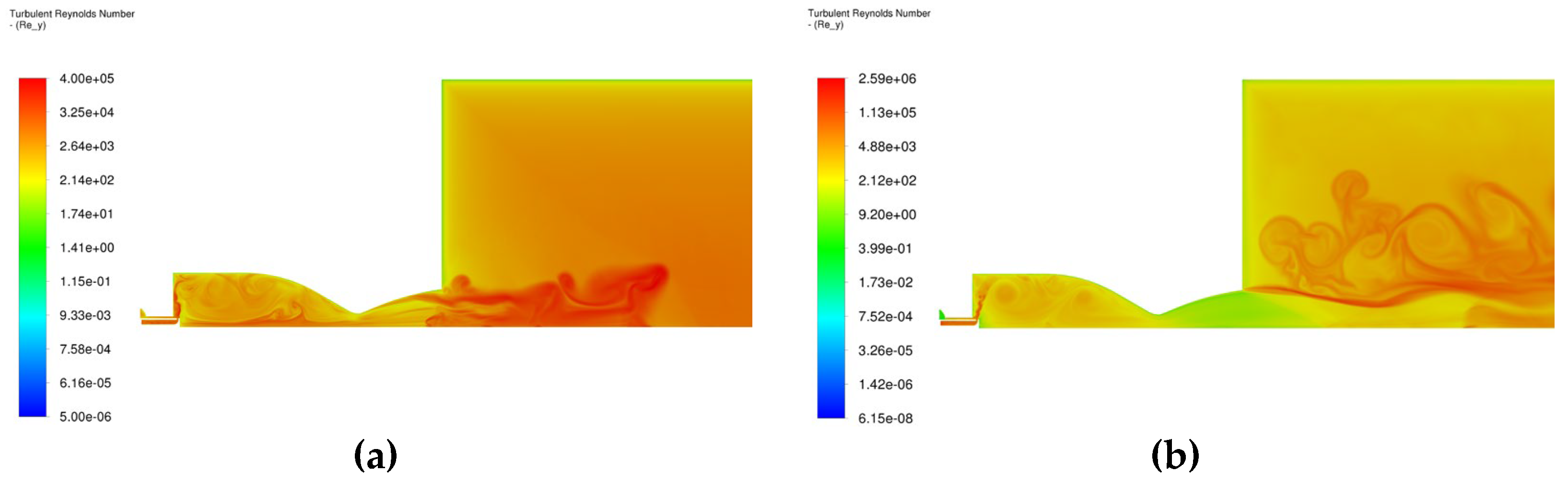
Figure 16.
Turbulent Reynolds number. a) 1 millisecond; b) 6 milliseconds
The increased mixing areas near the injector, highlighted by the high turbulent Reynolds number, implies that the injector induces turbulence effectively, stabilizing the combustion, a very well-known characteristic of the pintle type injector. The unburned hydrocarbons mass fraction reduction is also promoted through the induced turbulence by increasing their residence time inside the chamber. On the other hand, at later moments, the turbulent shear layer develops outside the nozzle (Fig. 15b) and leads to the dispersion of the species (Figs. 9b, 10b, 11b, 12b, 13b and 14b) above the jet discharge.
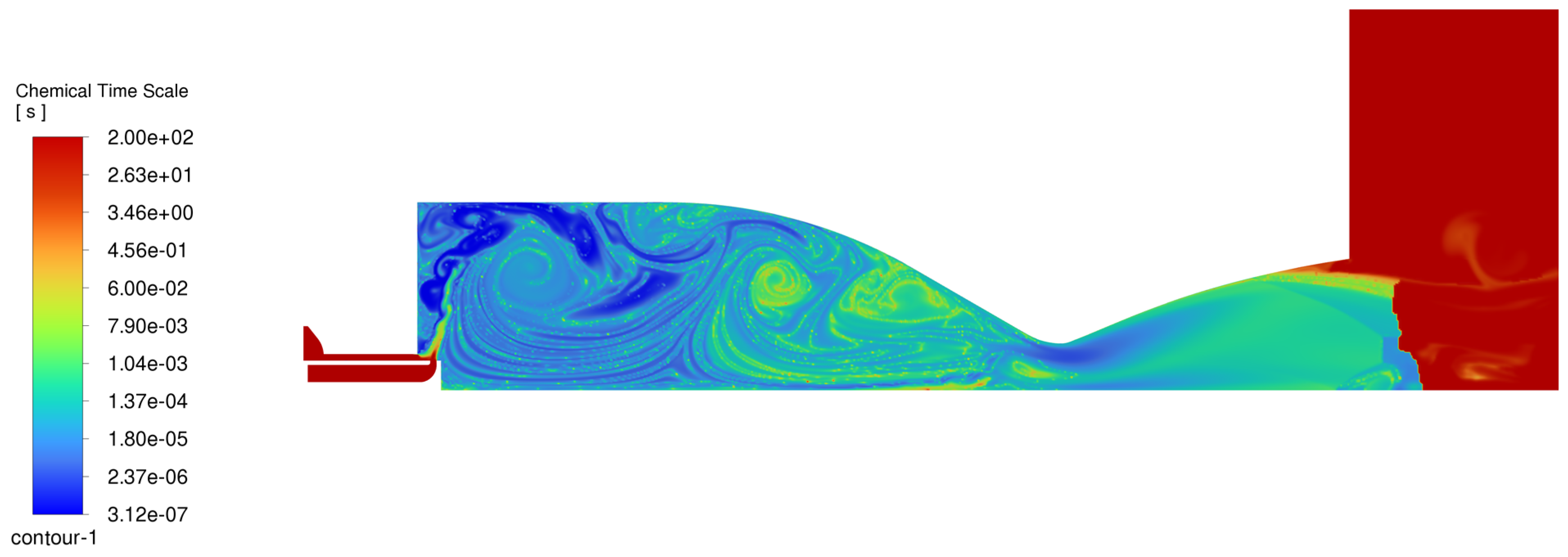
Figure 17.
Chemical time scale of the reaction (EDC-PaSR model) at 2.2 milliseconds flow time
The chemical time scale of the reaction, as determined using the EDC-PaSR model (Eq. 15), can be observed in a snapshot taken at 2.2 milliseconds flow time (after the ignition), in which the small-time scales show the fast reaction rates, while the longer time scale represents the slower reaction rates. Observing that in most of the combustion chamber the chemical time scale is small, combined with the high values of the turbulent Reynolds number (Fig. 16), it becomes apparent that flamelet-based turbulence-chemistry interaction models might be an appealing alternative.
The following graph shows the variation in the primary species, pressure and temperature with respect to flowtime in the exit section of the nozzle.
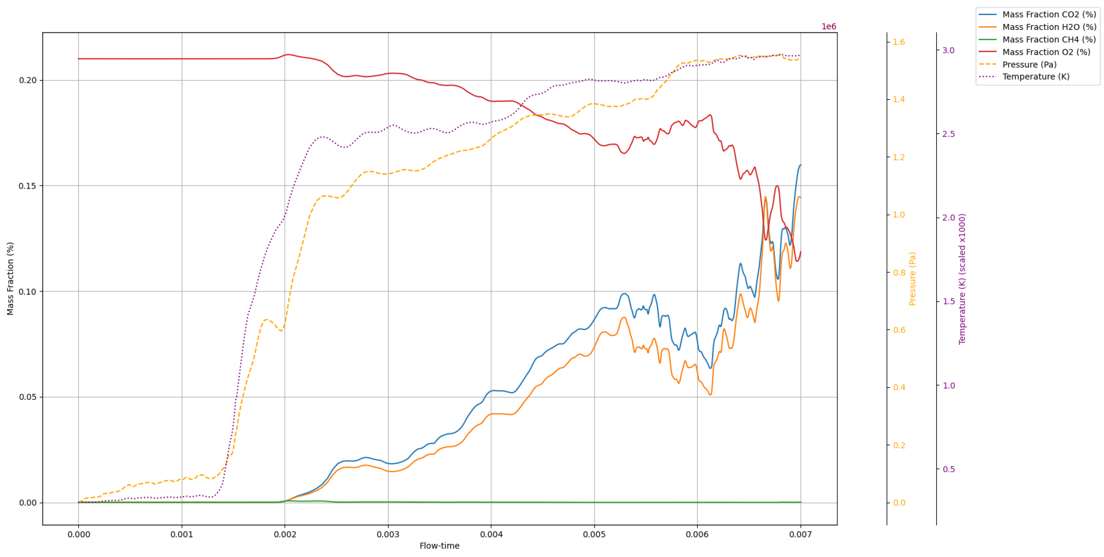
Figure 18.
Time history of the instantaneous area-averaged mass fraction, pressure and temperature at nozzle exit.
Figure 18.
Time history of the instantaneous area-averaged mass fraction, pressure and temperature at nozzle exit.
The temporal evolution of the primary species and combustion conditions in the ignition process provide indications regarding the trend of the flame front, which proves to be stable, with the CO2 and H2O concentrations rising sharply immediately after the ignition and stabilizing when getting closer to the steady state combustion.
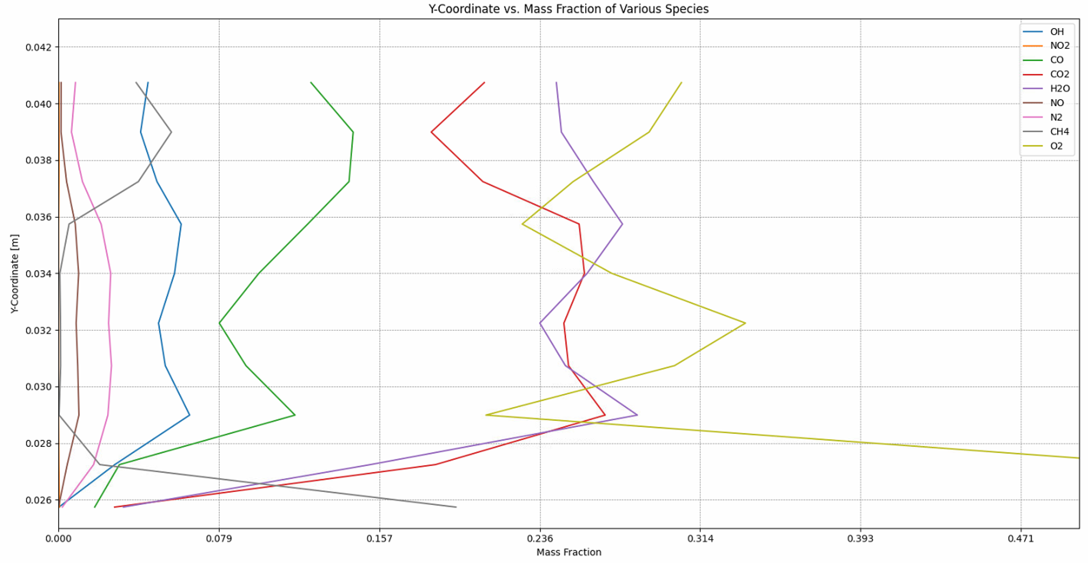
The species distribution along a probe line inside the combustion chamber can be observed in Figure 19 and Figure 20 at the same time stamps (1 and 6 milliseconds). The vertical probe line has been taken 27 mm from the pintle end wall. The illustrated profiles reflect a better introspection in the main recirculation zones in the mid region of the chamber. At 6 milliseconds, once the recirculation zones reached a mature state, an increase in the amount of product species and a sensible decrease in nitrogen concentration is noticed. This shows that the recirculation region is efficient in increasing the residence time of the reactants, thus increasing the combustion efficiency.
The pressure is slowly building up during the flame front propagation tending to reach the design value of 20 bar.
6. Discussion
Herein, salient features of the flame ignition and propagation processes in a rocket engine equipped with pintle injector have been investigated. The complexity of the numerical simulation has increased the computational burden such that only the first 6ms of the simulation were successfully accomplished. It is acknowledged that the steady state has not been reached and probably needs 10 more milliseconds. The spark ignition as it is implemented in Ansys Fluent in the framework of the EDC model seems to overestimate the temperature rise of the burnt gases, hence a limitation of the maximum temperature was required but only for a few time steps until the reaction mechanism has developed in a sufficient number of cells. Based on the instantaneous snapshots, it was estimated, for the first steps of the ignition process, a flame front velocity of about 180 m/s which from other simulations using FGM model is within the range of turbulent flame velocity. The presence of air trapped inside the chamber in the initial moments of the ignition generates substantial amounts of pollutants at engine start-up. The development of NOx species outside the chamber at the interface between the hot jet and ambient air could persuade researchers to develop strategies to treat the exhaust gases to mitigate the environmental impact. The present results represent a first step in the process of pintle performance optimization leading to a better, smooth mixing process to reduce the unburned hydrocarbons even further. The development of high quantities of carbon monoxide could mean, apart from imperfect mixing regions, that the length and/or width of the combustion chamber should be modified (most likely increased) for enhancing the residence time for CO/CO2 conversion. It becomes apparent that if this amount of CO is generated for a GCH4/GOX combustion then, for a two-phase (GCH4/LOX) combustion, the efficiency of the burning may drop even to lower values when vaporization is to be accounted for as well. Moreover, the uneven mixing regions, temperature distribution and flame front behavior observed in the CFD analysis have a direct impact on flame stability and thermal load on the exposed parts of the injector, particularly the pintle tip. Reducing the thermal load by film cooling might be the only alternative to thermal barrier coating. The identification of these zones through numerical simulation provides a direct insight into the operation of the engine and is the starting point in future design optimization process of the pintle injector, reducing the development costs generated by the need for iterative prototyping, at least in the early design stage.
It was noticed that real-gas approach in the form of Peng-Robinson equation of state, although, at first glance, not necessary as pressure was moderate, showed quite consistent departures from ideal gas behavior especially inside the pintle injector. The magnitude of this departure will increase with growing pressure and enforcing cryogenic conditions for oxidizer. Alternatively, a more complex chemistry-turbulence interaction model like FGM model may offer better insights in the intricate ignition and flame development process. Finally, depending on the computational resources, the complexity of the model can be raised to a large eddy simulation level.
A further comparison between EDC and FGM models would probably settle which approach is better for ignition simulation.
Author Contributions
Conceptualization, A.M and D.I; methodology, A.M.; Formal analysis, D.I.; Investigation, A.M.; Writing – original draft, A.M>; Writing – review & editing, D.I. All authors have read and agreed to the published version of the manuscript.
Funding
This research received no external funding.
Data Availability Statement
All data, models, or code that support the findings of this study are available from the corresponding author upon reasonable request.
Conflicts of Interest
The authors declare no conflict of interest.
References
- Mereu and D. Isvoranu, Joint design and simulation of GOX-GCH4 combustion and cooling in anexperimental water-cooled subscale rocket engine, INCAS Bulletin, vol. 15, no. 4, pp. 159–167, 2023, 2066-8201. [CrossRef]
- Gordon Dressler and J. Bauer, “TRW pintle engine heritage and performance characteristics”, 22 Aug 2012.
- Chang, Y.; Zou, J. Experimental and Numerical Study on the Ablation Analysis of a Pintle Injector for GOX/GCH4 Rocket Engines. Coatings 2023, 13, 1022. [CrossRef]
- Frassoldati, A.; Cuoci, A.; Faravelli, T.; Ranzi, E.; Candusso, C.; Tolazzi, D., “Simplified kinetic schemes for oxy-fuel combustion”, Sustainable Fossil Fuels for Future Energy—S4FE, Rome, Italy, 6–10 July 2009.
- V.M. Zubanov et al 2017 J. Phys.: Conf. Ser. 803 012187.
- Gerasimov, G.Y., Shatalov, O.P. Kinetic mechanism of combustion of hydrogen–oxygen mixtures. J Eng Phys Thermophy 86, 987–995 (2013). [CrossRef]
- Peters, N. Laminar diffusion flamelet models in non-premixed turbulent combustion. United Kingdom: N. p., 1984. Web. [CrossRef]
- Peters, Norbert. “Laminar flamelet concepts in turbulent combustion.” (1988).
- Donghyuk Kang, Sanghoon Han, Chulsung Ryu, Youngsung Ko, “Design of pintle injector using Kerosene LOx as propellant and solving the problem of pintle tip thermal damage in hot firing test”, Acta Astronautica 201 (2022) 48–58, ISSN 0094-5765. [CrossRef]
- Xin-xin Fang, Chi-bing Shen, “Study on atomization and combustion characteristics of LOX/methane pintle injectors”, Acta Astronautica 136 (2017) 369–379. [CrossRef]
- Son, M., Acta Astronautica (2017). [CrossRef]
- Frassoldati, Alessio et al. “Simplified kinetic schemes for oxy-fuel combustion.” (2009).
- De Giorgi, M.G.; Sciolti, A.; Ficarella, A. Application and Comparison of Different Combustion Models of High Pressure LOX/CH4 Jet Flames. Energies 2014, 7, 477-497. [CrossRef]
- van Oijen, Jeroen & Goey, Philip. (2000). Modelling of Premixed Laminar Flames using Flamelet-Generated Manifolds. Combustion Science and Technology - COMBUST SCI TECHNOL. 161. 113-137. [CrossRef]
- A. V. Brito Lopes, N. Emekwuru, E. Abtahizadeh; Flamelet generated manifold simulation of highly swirling spray combustion: Adoption of a mixed homogeneous reactor and inclusion of liquid-flame heat transfer. AIP Advances 1 November 2022; 12 (11): 115026. [CrossRef]
- Maria Grazia De Giorgi and Alessio Leuzzi. "CFD Simulation of Mixing and Combustion in LOX/CH4 Spray Under Supercritical Conditions," AIAA 2009-4038. 39th AIAA Fluid Dynamics Conference. June 2009.
- Ziguang Li, Peng Cheng, Qinglian Li, Pengin Cao. “Study on the formation and maintenance mechanism of the stationary flame at the head of a LOX/GCH4 pintle injector element”, Aerospace Science and Technology, 145. 2024.
- * * * ANSYS Fluent Theory Guide Release 2022 R1, January 2022.
- M. S. Gritskevich, A. V. Garbaruk, J. Schutze, F. R. Menter. "Development of DDES and IDDES Formulations for the k-ω Shear Stress Transport Model”. Flow, Turbulence and Combustion. 88(3). 431–449. 2012. [CrossRef]
- M.T. Lewandowski and I.S. Ertesvag. "Analysis of the Eddy Dissipation Concept formulation for MILD combustion modelling". Fuel. 224. 687–700. 2018. [CrossRef]
- M.T. Lewandowski, Z. Li, A. Parente, and J. Pozorski . "Generalised Eddy Dissipation Concept for MILD combustion regime at low local Reynolds and Damköhler numbers. Part 2: Validation ofthe model". Fuel. 278. 117743. 2020. [CrossRef]
- Gregory P. Smith, David M. Golden, Michael Frenklach, Nigel W. Moriarty, Boris Eiteneer, Mikhail Goldenberg, C. Thomas Bowman, Ronald K. Hanson, Soonho Song, William C. Gardiner, Jr., Vitali V. Lissianski, and Zhiwei Qin http://www.me.berkeley.edu/gri_mech/.
- V. Zimont. "Gas Premixed Combustion at High Turbulence. Turbulent Flame Closure Model Combustion Model". Experimental Thermal and Fluid Science. 21. 179–186. 2000. [CrossRef]
- V. Zimont,W. Polifke, M. Bettelini, and W.Weisenstein. "An Efficient Computational Model for Premixed Turbulent Combustion at High Reynolds Numbers Based on a Turbulent Flame Speed Closure". J. of Gas Turbines Power. 120. 526–532. 1998. [CrossRef]
- V. L. Zimont and A. N. Lipatnikov. "A Numerical Model of Premixed Turbulent Combustion of Gases". Chem. Phys. Report. 14(7). 993–1025. 1995.
- Mouze-Mornettas, M. Martin Benito, G. Dayma, C. Chauveau, B. Cuenot, et al.. “Laminar flame speed evaluation for CH4/O2 mixtures at high pressure and temperature for rocket engine applications”. Proceedings of the Combustion Institute, 39 (2), pp.1833-1840. hal-03841911, 2023. [CrossRef]
Figure 2.
a) Section view of the studied 1 kN reduced-scale gaseous rocket engine with the custom spark generator; b) Main dimensions of the injector.
Figure 2.
a) Section view of the studied 1 kN reduced-scale gaseous rocket engine with the custom spark generator; b) Main dimensions of the injector.
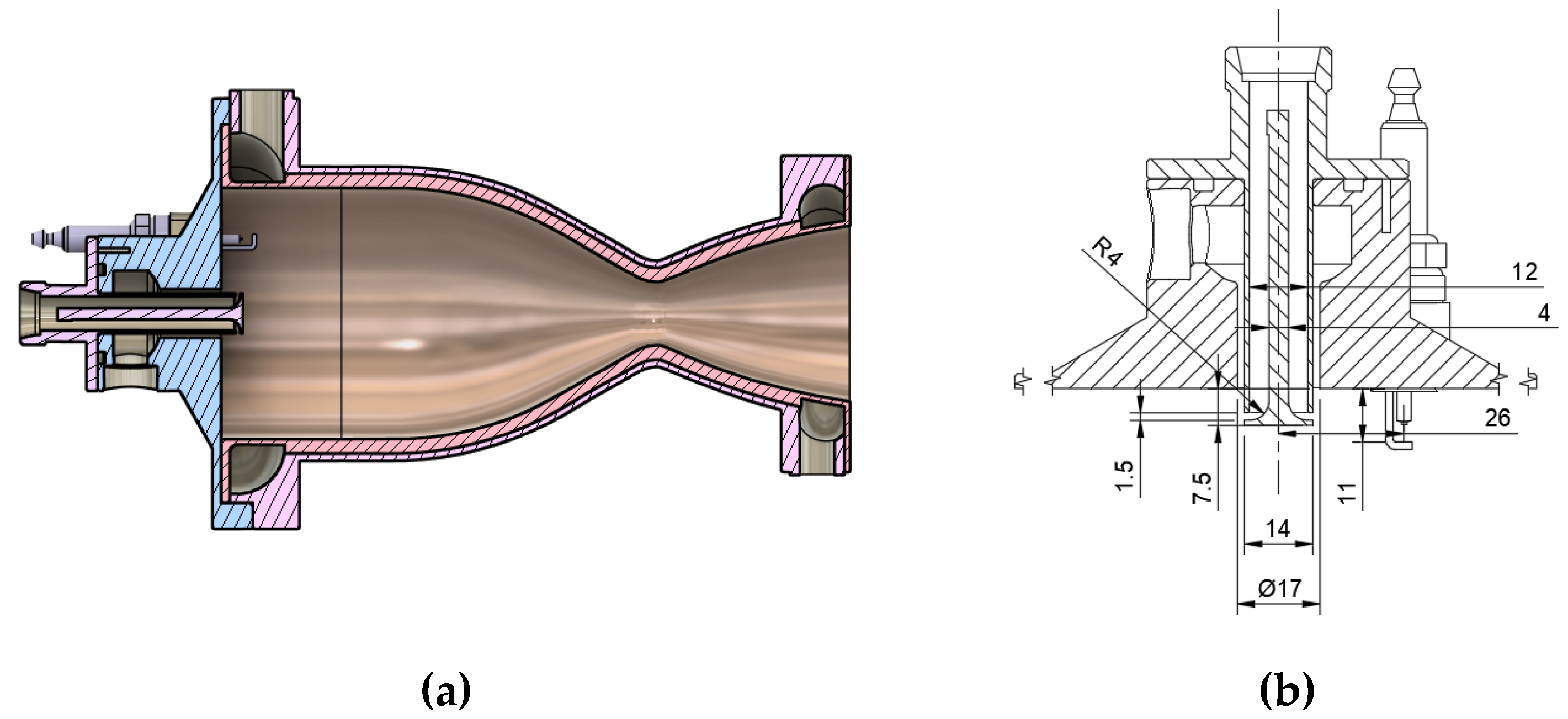
Figure 3.
Main dimension of the computation domain.
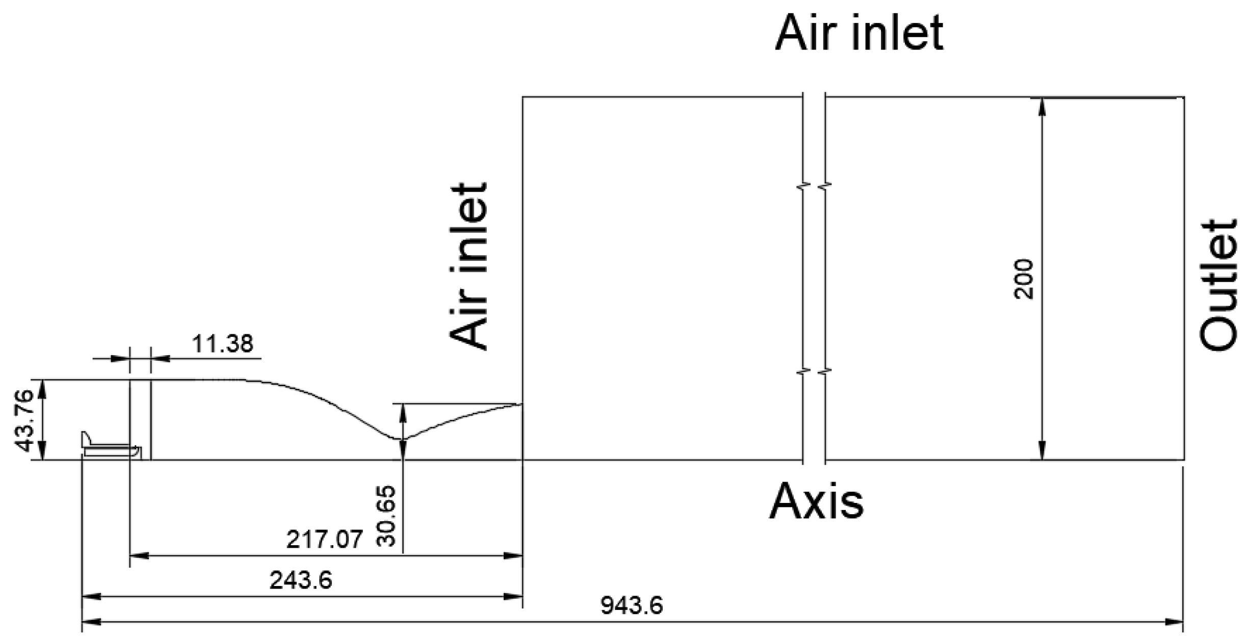
Figure 6.
Instantaneous temperature distribution during the first 0.3 milliseconds after initiation of the spark a) 0 millisecond, spark is initialized; b) 0.1 milliseconds; c) 0.2 milliseconds; d) 0.3 milliseconds.
Figure 6.
Instantaneous temperature distribution during the first 0.3 milliseconds after initiation of the spark a) 0 millisecond, spark is initialized; b) 0.1 milliseconds; c) 0.2 milliseconds; d) 0.3 milliseconds.
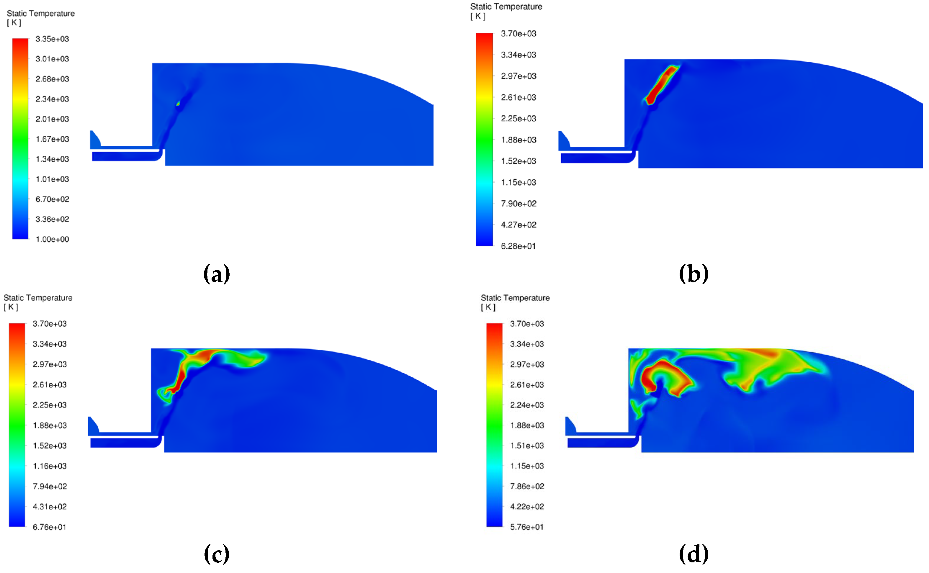
Figure 19.
Species distribution on the probe a line inside the chamber at 1ms.
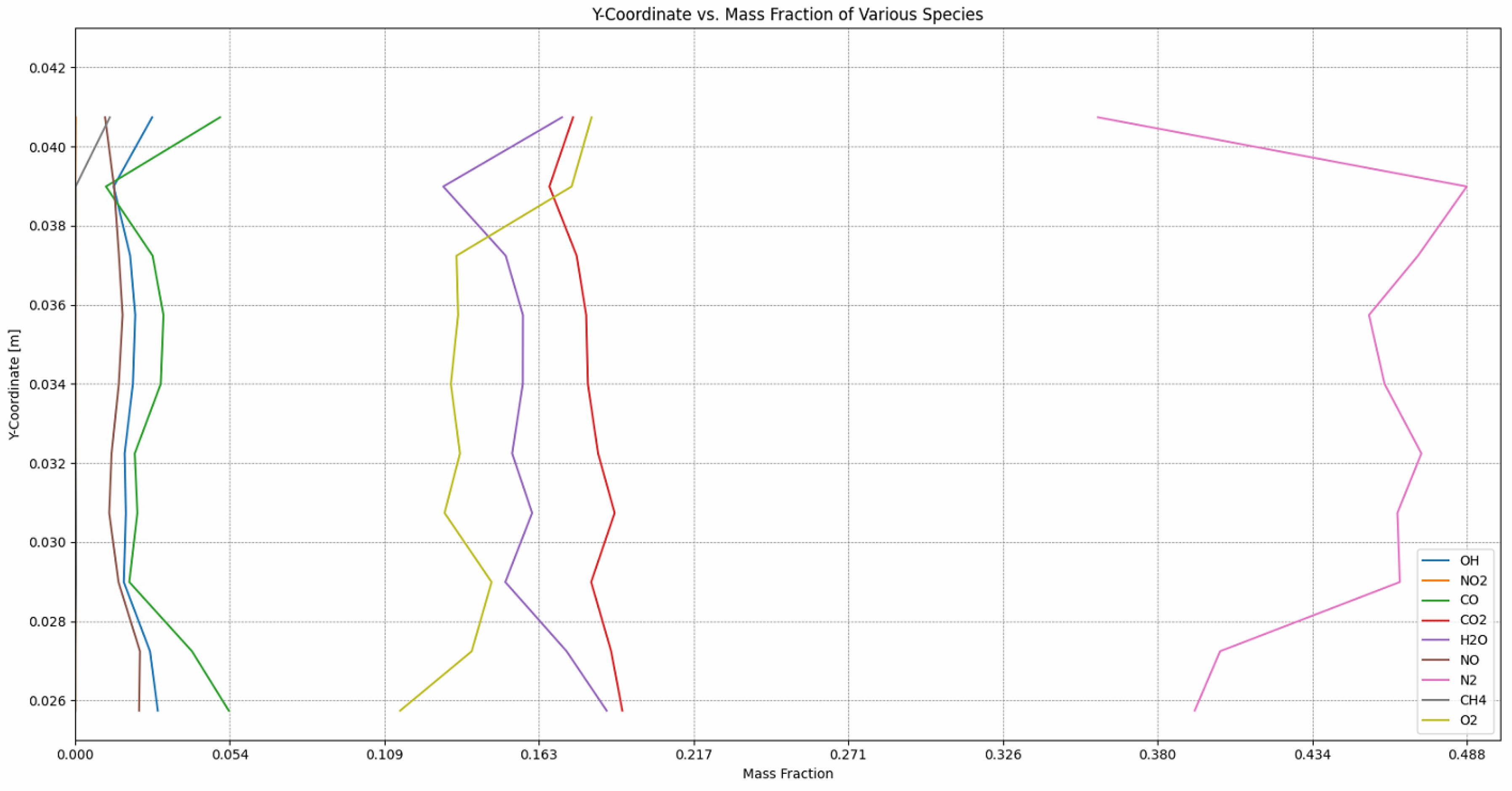
Figure 20.
Species distribution on the probe line inside the chamber at 6ms.
Disclaimer/Publisher’s Note: The statements, opinions and data contained in all publications are solely those of the individual author(s) and contributor(s) and not of MDPI and/or the editor(s). MDPI and/or the editor(s) disclaim responsibility for any injury to people or property resulting from any ideas, methods, instructions or products referred to in the content. |
© 2024 by the authors. Licensee MDPI, Basel, Switzerland. This article is an open access article distributed under the terms and conditions of the Creative Commons Attribution (CC BY) license (http://creativecommons.org/licenses/by/4.0/).
Copyright: This open access article is published under a Creative Commons CC BY 4.0 license, which permit the free download, distribution, and reuse, provided that the author and preprint are cited in any reuse.


