
Submitted:
22 September 2025
Posted:
23 September 2025
You are already at the latest version
Abstract
Turbulent diffusion (non-premixed) flames are commonly found in industrial burners, such as burners used in boilers and combustion furnaces. Bluff-body burners are one of three methods to stabilize turbulent diffusion (non-premixed) flames, where the separation wall between the core fuel jet stream and the surrounding oxidizer coflow stream serves as a flame holder. The flow solver “reactingFoam” of the open-source OpenFOAM software for control-volume-based computational fluid dynamics (CFD) modeling offers the capability of simulating reacting flows as encountered in turbulent diffusion flames. In the current study, we assess qualitatively and quantitatively the ability of this CFD solver for treating the reacting flow problem of a popular benchmarking bluff-body stabilized flame, that is, the HM1 flame. This HM1 turbulent non-premixed flame (TNF) has a fuel stream composed of 50% hydrogen (H2) and 50% methane (CH4) by mole. This fuel stream is surrounded by a coflow of oxidizing air jet. The acronym (HM) stands for “Hydrogen-Methane”. This flame was studied experimentally (experiment B4F3) at the University of Sydney (in the New South Wales state, Australia) using different techniques, such as laser Doppler velocimetry (LDV), Rayleigh scattering, and laser-induced fluorescence (LIF). A measurement dataset of flow and chemical fields was compiled and made available freely for validating relevant computational models. We simulate the HM1 flame using the reactingFoam solver and report here various comparisons between the simulation results and the experimental results to aid in judging the feasibility of this open-source CFD solver. Overall, we notice good agreement with the experimental data in terms of resolved profiles of the axial velocity, mass fractions, and temperature. This study, and the presented details about the reactingFoam solver and its implementation, can be viewed as a good case study in CFD modeling of reacting flows. In addition, the information we provide about the measurement dataset, the emphasized recirculation zone, the entrainment phenomena, and the irregularity in the radial velocity can help other researchers who may use the same HM1 data.
Keywords:
bluff-body burner
; combustion
; diffusion flame
; HM1
; OpenFOAM
1. Introduction
1.1. Flame Types
A flame is a self-sustaining zone of a combustion and heat release process. Such a flame is produced when a burnable substance (fuel) undergoes exothermic oxidation reactions with an oxidizer [1]. Flames represent a localized phenomenon. Therefore, they occupy a small portion of the combustible substance (fuel) at a given instance instead of taking place uniformly throughout that entire substance [2]. Typically, flames form as a result of reactions between gaseous primary reactants (the fuel and oxidizer) [3,4]. If the fuel is liquid, it undergoes local vaporization and forms a flammable gas before combustion occurs [5]. If the fuel is solid, it undergoes local pyrolysis and breaks down into a flammable gas before combustion occurs [6].
Based on the mixing process between the oxidizer and the fuel, it is possible to classify flames into two main categories [7].
The first flame type according to this classification is the premixed flame. In this type, the fuel and the oxidizer mix and form a homogeneous gas mixture before reaching the combustion zone [8]. Such premixed flames can be visually identified due to being non-luminous and translucent, having pale colors typically varying from yellow to green [9]. The reason that premixed flames tend to be non-luminous is the absence of the incandescent soot particulates [10,11]. This, in turn, is attributed to the consumption of generated soot particles in a premixed flame as they meet the oxidizer available within the flame and react with it [12]. Therefore, premixed flames tend to have a small amount of soot [13]. A famous example of premixed flames is the core of the blue conical flame of the Bunsen burner that is found in laboratory settings [14]. The flame found in most spark-ignited automotive engines is another example of premixed flames [15]. Also, the inner cone of an oxy-acetylene gas welding flame is a good example of premixed flames, where the mixing happens inside the welding torch [16].
The second type of flame, based on the fuel-oxidizer mixing, is the diffusion flame (also called a non-premixed flame). Such a flame is called “non-premixed” because the oxidizer and the fuel are introduced into the combustion zone as separate streams without prior mixing [17]. On the other hand, the name “diffusion” arises from the fact that the chemical reactions take place only where the fuel and the oxidizer are mixed [18] at the molecular level via differential molecular diffusion (DMD) [19]. In non-premixed flames, the time scale of chemical reaction is much smaller than the time scale for molecular diffusion. In other words, reaction is much faster than diffusion. As a result, molecular diffusion becomes the rate-limiting phenomenon [20] because the fuel and oxidizer diffuse into each other relatively at a much slower rate than their chemical reaction. Hence, non-premixed flames are named after the rate-controlling step of their formation, which is diffusion and mixing on a molecular scale [21]. Thus, non-premixed flames usually propagate and burn more slowly than premixed flames [22]. Diffusion (non-premixed) flames are commonly characterized by the release of soot particles [23]. This feature is caused by the insufficient oxidizer within the flame zone, resulting in the famous orange luminous color of such flames. Non-premixed flame burners often have larger flames than premixed flames, and typically exhibit more uniform temperature distribution (lower peak temperature) and heat flow [24]. These burners, known for their high heat production and efficiency, are designed to ensure the complete combustion of the fuel oil, thus reducing emissions [25]. Compared to premixed flames, non-premixed flames are encountered much more frequently in daily life [26]. Examples of non-premixed flames include matchstick flames, candle flames, open fires, the outer cone of the flame of the Bunsen burner [27], and the outer envelope of an oxy-acetylene gas welding flame [28].
Flames can also be categorized based on the regime of their movement, which can be laminar or turbulent [29]. The core of the flame in the case of a Bunsen burner represents a laminar premixed flame [30]. The flame of a candle and the outer cone of the flame in the case of a Bunsen burner are representative of laminar non-premixed flames [31]. Turbulent flames are often found in practical and larger applications [32], such as power generation [33] and thermal industrial processes [34]. Commercial-scale combustion [35] demands high speeds of supply for the reactants [36]. Such speeds exceed the thresholds of a laminar flame remarkably. Laminar flames are of special importance in academic research because they are simpler and easier to characterize and understand [37]. Laminar flames allow for building mathematical models for the flame combustion process, which can be extended afterwards to the more complex turbulent flames [38].
1.2. Turbulent Non-Premixed Flames
Turbulent non-premixed flames (TNF) combine the complexity of turbulence and the challenge of properly mixing the individual reactant streams [39]. Despite this, turbulent non-premixed flames are favored over premixed flames in a large number of industrial systems [40] due to two reasons:
First, non-premixed burners are simpler to design and build than premixed burners [41]. This is due to the higher tolerance of the reactant proportions for achieving a desired level of mixing [42]. There are no premixing requirements for non-premixed burners [43].
Second, non-premixed burners are safer to operate than premixed burners. This is because non-premixed burners do not exhibit flashback or autoignition in undesirable locations [44].
With turbulence introduced in turbulent non-premixed flames, the term “diffusion” that strictly applies to the differential molecular diffusion of chemical species remains the controlling mechanism. Initially, macroscopic turbulent convection is responsible for mixing the fuel and the oxidizer. Eventually, molecular diffusion completes the mixing process at the microscopic scale, such that chemical reaction can happen [45].
1.3. Instability of Turbulent Non-Premixed Flames
High jet speeds in turbulent non-premixed flames seem commercially attractive because they permit a high heat duty [46]. Such high-velocity burners are found in the aluminum, steel, or glass industries. However, such an approach to intensify the flame tends to make the flame unstable, where undesirable phenomena such as blow-off and lift-off appear. Lift-off refers to the phenomenon where the flame is detached from the burner, and an intervening zone of turbulent pre-mixing is established between the flame and the burner [47], as a result of excessive speed of the jet [48]. At larger jet speeds, the flame is extinguished, which is the blow-off phenomenon [49]. Either phenomenon (lift-off or blow-off) is undesirable and is considered a deviation from the stable attached flame [50].
High velocity burners in furnaces have another advantage beyond the intensified heating rates, which is environmental [51]. These burners produce low NOx (nitrogen oxides) emissions, mostly nitric oxide (NO) [52]. This happens because these burners inherently entrain significant amounts of cool furnace gases that are injected into the flame envelope before the complete combustion [53]. This results in reducing the average in-flame temperature, which hinders the high-temperature thermal formation of NOx [54]. This thermal formation of nitrogen oxides requires high temperatures (above 1,200 °C) to allow the molecular nitrogen gas (N₂) and the molecular oxygen gas (O₂) in the air to dissociate [55] into atomic nitrogen gas (N) and atomic oxygen gas (O) [56]. The atomic oxygen reacts with the molecular nitrogen, and the atomic nitrogen reacts with the molecular oxygen and forms nitric oxide (NO) [57].
Alternatively, reducing the environmentally-harmful NOx emissions [58] can be achieved by controlling the combustion conditions [59]. For example, enforcing lean fuel concentration also lowers the temperature and reduces the emissions [60]. However, this approach is considered harsh, and it increases the chance of flame instability [61].
1.4. Stabilizing Turbulent Non-Premixed Flames
Stabilizing high-jet turbulent non-premixed flames (this means anchoring the flames to the burner) in industrial burners can be achieved through three methods [62].
One of these stabilization methods uses a pilot burner (also called a pilot light) [63] as an active stabilization technique [64]. This technique involves adding a small auxiliary flame that burns initially in order to ignite the main burner [65]. The pilot flame can later be deactivated if the main flame does not show signs of instability [66]. However, the pilot flame is kept in continuous operation if this is necessary to avoid extinction of the main flame, thus to maintain a stable burner operation [67]. The auxiliary pilot flame can be implemented in the form of an electric igniter or in the form of a small premixed flame. Pilot-stabilized turbulent non-premixed flames (TNF) are known to be very stable over a wide range of operational conditions [68]. Nevertheless, pilot-stabilized turbulent non-premixed flames imply the penalty of installing and maintaining the additional pilot burner [69]. Also, there is extra energy consumption (either in the form of electricity or fuel) [70] to enable the pilot-flame stabilization method.
Another stabilization method for high-jet TNF utilizes swirl or recirculation, which is a passive technique (this means it does not consume external energy) [71]. In this method, a recirculation zone is carefully introduced such that it provides favorable conditions for the chemical reactions to take place. However, this swirling technique can be accompanied by unfavorable effects because a precessing vortex core can lead to combustion instability. Furthermore, the introduced swirl affects the unsteady location where the flame is anchored. Therefore, further combustion instabilities may occur, and this was observed experimentally for a gas turbine combustor [72].
The third TNF stabilization method is the method we explore in the current study. It is also a passive one. It. This method is the utilization of a bluff-body burner with a central fuel jet. This burner type is also called a flame holder [73]. This burner is characterized by a flat or a block-shaped object, which is the bluff body [74]. This bluff body helps in establishing a zone of low-speed hot recirculation zone [75]. When this bluff body is placed in the fast jet streams of the reactants, the flow is slowed down and heated, and this enables the chemical reactions to proceed toward ignition. Bluff-body non-premixed burners are particularly important in several industrial applications. Bluff body burners are also used in premixed flames [76,77]. Therefore, it is very useful to have simulation and design tools that are reliable for analyzing and predicting the flow fields and compositional profiles of the produced flames [78]. Bluff-body turbulent non-premixed flames burners serve as a good benchmarking case [79] for computational combustion modeling because they form a reasonable trade-off between the complication level associated with real, more sophisticated combustors and the relative simplicity and clear boundary conditions for modeling purposes.
1.5. HM1 Flame
The bluff-body stabilized flame adopted here as a benchmarking case for modeling is called the HM1 flame. It is an axisymmetric turbulent non-premixed flame that was studied experimentally at the University of Sydney [80]. It has been referenced online by the TNF Workshop Series [81,82,83,84,85] of the International Workshop on Measurement and Computation of Turbulent Non-premixed Flames [86].
This flame is assigned the name “HM1” because of the chemical composition of the gaseous fuel stream, which is composed of molecular hydrogen (H2) and methane (CH4) with equal volume fractions of 50% each (1:1 molar ratio). The burner is surrounded by a coflow of air. The HM flame family has three members: (1) HM1 flame, which has a fuel jet speed of 118 m/s, (2) HM2 flame, which has a faster fuel jet of 178 m/s, and (3) HM4 flame, which has a faster fuel jet of 214 m/s [87].
Given the 50%/50% volume composition (mole fractions) of CH4 and H2 in the fuel, the corresponding mass fractions are 8/9 or 0.8889 for methane (CH4) and 1/9 or 0.1111 for molecular hydrogen (H2) [88]. These mass fractions are based on molecular weights of 16 kg/kmol for methane [89] and 2 kg/kmol for molecular hydrogen [90]. The mixture’s molecular weight can be computed based on these data as the arithmetic mean of the two molecular weights, which is 9 kg/kmol.
The HM1 flame’s experiment is also assigned the code name “B4F3” by the experimental investigators at the University of Sydney, who are members of the Clean Combustion Research Group at the School of Aerospace, Mechanical and Mechatronic Engineering (AMME) [91].
The HM1 flame is an attractive benchmarking problem for computational fluid dynamics (CFD) solvers. This is due to the practicality of its high-velocity bluff-body burner as well as the detailed information about the burner, the flow settings, and the measurement process. This information allows for establishing a reasonably equivalent computational model with less deviation from the actual geometric or input conditions. In addition, the detailed experimental information for the HM1 flame is useful for making a non-ambiguous interpretation of the experimental data. These features of the HM1 flame consequently lead to meaningful and consistent assessment of the similarity between the CFD results and the experimental results.
1.6. Some Computational Studies About the HM1 Flame
The HM1 bluff-body stabilized turbulent non-premixed benchmarking flame considered in the current study has been utilized in earlier computational works.
For example, Yan et al. [92] solved the axisymmetric governing equations for this flame using a general-purpose computational fluid dynamics (CFD) computer code that employed a multi-block structured grid that was constructed based on general non-orthogonal coordinates and the finite volume methods (FVM) [93]. The non-uniform grid consisted of three blocks with a total of approximately 18,000 cells, which were distributed more densely near the bluff-body burner. They used the flamelet model for representing the turbulence-chemistry interaction (TCI) [94]. Their primary goal was to examine the influence of the turbulence model on the overall numerical predictions. They explored three different turbulence models, which are: (1) the basic k-epsilon () model, (2) a modified k-epsilon model () with a varied anisotropy parameter, and (3) the explicit algebraic stress model (EASM) [95,96]. It is worth mentioning that the coefficient in their basic k-epsilon model was 1.83, which is slightly below the standard value of 1.92 [97]. The researchers found that the numerical predictions depend on the selected turbulence model. Their numerical predictions were generally satisfactory, despite notable deviations in the radial profile of the root mean square (RMS) of the axial velocity fluctuations, the root mean square (RMS) of the mixture fraction variance, and the average mass fraction of carbon dioxide (CO2) for each of the three turbulence models attempted.
Another research team, Liu et al. [98], treated the problem as axisymmetric also. However, they employed a single-block structured grid with a total of 6,912 cells (72 cells along the axial direction and 96 cells along the radial direction). They modeled the turbulence-chemistry interaction (TCI) through the joint probability density function (PDF) technique [99]. This research team investigated the sensitivity of their numerical predictions to the mixing model for the probability density function calculations. This mixing model represents the influences of molecular diffusion. The research team tried two different mixing models, which are (1) the interaction by exchange with the mean (IEM) model [100,101], and (2) the Euclidean minimum spanning tree (EMST) [102]. Some numerical results of the radial profiles of the mean mixture fraction and its root mean square (RMS) values showed strong deviations near the burner’s centerline. It was observed that the model gave much lower values than the experimental values.
In another study, Odedra and Malalasekera [103] again treated the HM1 flame as an axisymmetric problem in their numerical modeling. They performed Favre-averaged Navier Stokes (FANS) simulations using steady and unsteady flamelet models. The time-dependence was captured through a post-processing technique using the Eulerian particle flamelet model (EPFM) [104]. They implemented their simulations using the commercial computational fluid dynamics software Ansys Fluent [105]. In their simulations, they selected the Reynolds stress model (RSM) [106] for representing the turbulence effects. Excluding a small upstream extension, the main computational domain was discretized into 44,200 (260 axially × 170 radially) quadrilateral cells. The computed radial profiles of the axial velocity were found to be in good agreement with the experimental data. However, the radial velocity profiles showed big deviations from the experimental data. The computed mass fraction of molecular hydrogen (H2) as a reactant component was over-predicted near the centerline. Nevertheless, the computed results quickly became aligned with the experimental data as the distance from the centerlines increased.
Wang et al. [107] used a modified version of the HM1 flame as a representative test case to examine the finite-rate chemical reaction in the case of a specialized MILD (moderate or intense low oxygen dilution) combustion [108], with a Jet-into-Hot-Coflow (JHC) burner. They investigated the differences between the environmentally-attractive [109] reduced-temperature low-pollution (low-NOx) MILD combustion and the conventional hot-temperature combustion. These differences include the dissimilarities in the flame characteristics. They used joint velocity-frequency-composition transported probability density function (TPDF) simulations, combined with a sensitivity analysis. It should be noted that their modeling does not correspond to the original HM1 flame we refer to here, but to a variant of it, since the burner they modeled has a MILD JHC [110] design that is different from the original experimental configuration, and also the coflow was oxygen-enriched. The coflow is a hot exhaust gas with oxygen and nitrogen. The chemical composition of that oxidant coflow, in the form of mass fractions, was 0.065 H2O, 0.055 CO2, 0.030 O2, and 0.850 N2 [111]. The research team attempted to maintain some features of the HM1 flame, such as the 1:1 volumetric ratio of the molecular hydrogen (H2) and methane (CH4).
In the studies of Raman and Pitsch [112], Kempf et al. [113], James et al. [114], and Chen et al. [115], the HM1 benchmarking flame was modeled using the computationally demanding [116] large eddy simulation (LES) method with a three-dimensional geometry. Given the large computational resources and time demands involved in this modeling method, these studies are considered less practical and more academic than strategies aimed at general engineering and industry problems [117].
In our computational fluid dynamics (CFD) simulations, we report here for the HM1 flame, we use a simplified axisymmetric geometry, which is adequate for this axisymmetric flame. We solve the FANS (Favre-averaged Navier Stokes) governing equations using the reactingFoam solver, which is part of the open-source software OpenFOAM (Open Field Operation And Manipulation) [118]. Our assessment of the open-source reactingFoam solver provides the interested researchers with a source of information to assess the solver and make a guided decision about the solver’s capabilities and limitations when modeling turbulent non-premixed flames (TNF) or related problems involving reactive gases and combustion. This assessment is achieved both qualitatively by visually comparing axial and radial profiles of velocity, chemical, or thermal field variables along different positions within the flame region, and quantitatively through computed aggregate deviation scalar quantities, such as the mean absolute deviation (MAD).
2. Experimental Geometry of the HM1 Flame
Figure 1 shows a schematic of the experimental cylindrical HM1 burner. The burner is situated inside a wind tunnel whose cross-section is a square. Despite the enclosing wind tunnel walls, the separation between the burner’s centerline and the wind tunnel walls is large enough to make the HM1 flame effectively open (not confined) [119]. The burner has a flat annular bluff-body face, with a fuel jet nozzle located in the center.
The fuel nozzle (orifice) has a diameter of 3.6 mm, while the outer burner diameter is 50 mm. The diagonal distance between the two opposite corners of the wind tunnel is 431.3 mm, while the perpendicular face-to-face distance is 305 mm. The cross-sectional area of the wind tunnel is 93,025 mm2, while the cross-sectional area of the burner’s circular cross-section (including the fuel nozzle) is 1.963.5 mm2, and the fuel nozzle’s area is 10.179 mm2. Thus, the area ratio of the wind tunnel to the burner to fuel nozzle is 47.3772:1.0000:0.0052 or 9139.13:192.90:1.00. These ratios indicate the big differences between the three areas.
The relatively large annular area of the bluff body (193 times the area of the fuel jet) results in forming a recirculation zone in which high-temperature gases are located, which are sufficiently hot to stabilize the flame by keeping it attached to the burner.
In a turbulent non-premixed (diffusion) flame (TNF), if the fuel jet speed increases and reaches a threshold limit (the blow-off speed), then the flame can be extinguished. This flame extinction happens downstream of the recirculation zone. The extinguished flame may reignite at a further downstream point. From the data given in Table 1, it can be seen that the HM1 flame is approximately at 50% of the blow-off threshold. Therefore, this blow-off instability is not encountered.
Figure 2 is a photo of an HM flame [121]. It is noticeable in the photo that this turbulent non-premixed flame (TNF) has a blue color rather than the more expected luminous orange color for non-premixed flames due to soot incandesce. The explanation of the uncommon blue color is also the explanation for blending methane (CH4) with molecular hydrogen (H2) in the HM family of flames. The presence of hydrogen in this fuel blend reduces the soot formation compared to burning pure methane or natural gas [122,123]. The suppression of soot formation in the synthetic CH4/H2 fuel is aligned with the formation of a recirculation zone that is nearly clean from soot [124]. The addition of hydrogen results in a carbon dilution effect (changing the concentration of carbon per unit mass of the fuel), which in turn causes a change in the distribution of the temperature field within the flame [125]. The addition of hydrogen also inhibits soot precursor species, such as acetylene or ethyne (C2H2) and polycyclic aromatic hydrocarbons (PAHs) [126]. The flames of pure methane or natural gas (without hydrogen blending) generally exhibit the formation of soot in the recirculation zone. As this formed soot is carried downstream (upward) [127], it undesirably interferes with the Raman signal. This interference harmfully affects the accuracy of the measured species mass fractions. Adding hydrogen to methane satisfactorily frees the recirculation zone from the undesirable soot.
In the experimental setting, the measurements of the axial velocity component and the radial velocity component were made concurrently using the non-intrusive optical technique of laser Doppler velocimetry (LDV) [128], with a two-color argon-ion laser beam having a power of 5 W [129]. This laser type has two major emission lines, one at 488.0 nm (blue) and another at 514.5 nm (green) [130,131].
3. Computational reactingFoam Model
3.1. Overview of OpenFOAM and reactingFoam
Our computational modeling for the HM1 flame was conducted using the computational fluid dynamics (CFD) solver reactingFoam [135]. This solver supports multi-species finite-rate chemistry, thermodynamics, flow turbulence, and turbulent combustion models. The solver is widely used in the combustion community [136]. The solver reactingFoam is one of several CFD solvers distributed under the OpenFOAM open-source software, which is a collection of computer codes written using the object-oriented programming (OOP) concepts [137] and the principles of the C++ programming language. The computer codes are augmented with various text files that serve as conveniently-editable datasets and lookup input files [138,139] for describing the computational geometry, defining the boundary conditions, setting the initial conditions, determining the physical modeling parameters, selecting the desired numerical solver settings, computing needed fluid properties, and listing the chemical reaction steps.
3.2. Main Governing Equations
The scalar mass conservation equation, the vector momentum conservation equation, the scalar species mass conservation equation (expressed in terms of the mass fraction), and the scalar energy conservation equation (expressed in terms of the static specific enthalpy) in the reactingFoam solver, respectively, are [140,141]
These equations apply to a compressible turbulent gaseous mixture. They are the Favre-averaged Navier Stokes formulation (FANS), which is theoretically derived based on density-weighted averaging of field variables [142]. The FANS formulation here is extended to a multi-species reacting gas. They are also called compressible Reynolds-averaged Navier-Stokes (RANS) equations [143].
In the above partial differential equations, a single arrow above a variable’s symbol means that it is a vector field, while a double arrow means that it is a tensor field.
The density is denoted by the symbol , the velocity vector is denoted by , the effective dynamic viscosity (sum of molecular viscosity and eddy viscosity) [144] is denoted by , the static pressure is denoted by , the turbulent kinetic energy per unit mass is denoted by , the effective kinematic mass diffusivity of the ith gaseous species in the mixture is denoted by , the mass fraction of the ith gaseous species in the mixture is denoted by , the reactive volume fraction [145] (which is a positive dimensionless scaling multiplier bounded by an upper limit of 1.0) is denoted by , the unscaled chemical reaction source [146] of the ith gaseous species is denoted by , the mixture’s static specific enthalpy is denoted by , the static specific enthalpy of the ith gaseous species is denoted by , the effective dynamic thermal diffusivity is denoted by , and the total number of gaseous species in the mixture is denoted by .
In the momentum equation, Equation (2), the operator ( is the trace of a tensor. The identity tensor in that equation is denoted by . The superscript () is the transpose operator.
In the static-enthalpic energy equation, Equation (4), the term is the substantial time derivative of the static pressure [147]. The last term of that equation was added as a differential diffusion term. It represents the difference between the species’ effective mass diffusivity and the mixture’s effective thermal diffusivity. This term implies the assumption of a unity molecular Lewis number and unity turbulent Lewis number for each gaseous species in the mixture [148]. The Lewis number is the ratio of the thermal diffusivity to the mass diffusivity [149]. It is admitted that this differential diffusion effect is generally neglected when modeling turbulent reacting flows [150].
All flow variables are stored at the cell centers (the center of the control volumes), rather than the cell’s face centers. However, spatial interpolation is heavily implemented during the simulation in order to compute the needed cell’s face values of the variables as temporary quantities. With this spatial scheme, the computational mesh (grid) is described here as having a collocated, rather than staggered, layout [151]. Collocated-mesh (CM) layouts are often favored over staggered-mesh (SM) layouts in the case of turbulence simulations [152]. Compared to staggered grids, collocated grids have the advantages of being easier to extend for three-dimensional nonorthogonal grids and allowing for better treatment of the domain boundaries in the case of body-fitted grids [153].
3.3. Turbulence-Chemistry Interaction
The turbulence-chemistry interaction (TCI) in our simulations is based on the Chalmers’ partially stirred reactor (CPaSR) model [154]. We adopted a minor variant of the standard k-epsilon model for modeling the unresolved turbulent scale. The minor improvement change adopted here is increasing the value of the model parameter () from the standard level of 1.44 to a slightly higher level of 1.60. This 11.1% increase is introduced because it better suits problems with self-similar round jets as the one encountered here [155]. In addition, this adjustment was found to yield favorable numerical stability [156].
With the simplifying assumption of unity laminar Schmidt numbers and unity turbulent Schmidt numbers for each species, can be replaced by in Equation (3) and Equation (4). The modified versions of these two equations, respectively, are
3.4. Pressure-Velocity Coupling
Our simulations adopt the PISO (Pressure Implicit Splitting of Operators) coupling scheme for the pressure and velocity [162]. In the PISO pressure-velocity coupling scheme, the primitive form of the continuity equation, Equation (1), is not directly solved. Instead, mathematical manipulation is performed to give two derived equations. The first derived equation is a Poisson-type elliptic partial differential equation (PDE) for the pressure. The source term in this derived PDE depends on the velocity vector. The second derived equation is an explicit expression for the velocity vector, which relates the velocity vector to the gradient vector of the pressure.
To better explain the PISO pressure-velocity coupling scheme, we consider the case of an incompressible fluid [163]. Writing a semi-discretized version of the vector momentum equation, Equation (2), gives [164]
where is a fixed-value coefficient for each cell, and it does not change over time. This coefficient depends on the geometry and discretization scheme used for the momentum equation [165]. This coefficient is the multiplier quantity for the cell’s own velocity vector . The source vector function is vector that accounts for the discretized terms of the momentum equation while excluding the pressure gradient. This means that this vector source function accounts only for the transport part of the momentum equation.
The derived implicit elliptic equation for the pressure and the companion derived explicit equation for the velocity vector correction can be obtained directly from Equation (7). Respectively, these two derived equations of the PISO scheme are
It can be noticed that Equation (9) is very similar to Equation (7). Both sides of Equation (7) were divided by to reach Equation (9), which strengthens its nature as an explicit equation. Also, the right-hand side velocity vector in Equation (9) has a temporary (predicted) velocity vector that needs a corrector step in order to become a corrected velocity vector in the left-hand side.
From Equation (9), it is possible to derive Equation (8) after applying the divergence operation to both sides of the equation, and then enforcing the condition that the corrected velocity field has zero divergence, which is mathematically expressed as
The vector momentum equation, Equation (2), is solved initially using the latest existing pressure field. This yields a temporary velocity vector field that does not necessarily satisfy the continuity equation.
This predictor stage is followed by a three-step PISO corrector stage, which is described as follows:
- First, the elliptic pressure equation, Equation (8), is solved to give a pressure field.
- Second, the mass fluxes at the cell faces are updated using the obtained pressure field.
- Third, the temporary velocity vector field obtained during the predictor stage is corrected using the explicit expression in Equation (9). This takes into account the newly resolved pressure field.
The above sequence represents a single PISO correction step [166]. It can be repeated for improved performance.
For the overall solution procedure, the governing equations are corrected five times per time step in a sequential manner [167,168]. Within each of these “outer” corrections, two PISO “inner” corrections are performed.
Therefore, the following governing equations are solved five times in each time step:
- Momentum equation
- Species mass-fraction equations
- Energy equation
On the other hand, the following governing equations are solved ten times in each time step:
- Elliptic pressure equation
- Explicit velocity vector correction equation
The following solution order takes place in the computational algorithm during a single “outer” loop:
- 4.
- The momentum equation, Equation (2), is solved.
- 5.
- The species equations, Equations (5), are solved.
- 6.
- The energy equation, Equation (6), is solved.
- 7.
- The PISO correction “inner” loop is performed.
For each implicit equation (all field equations except the velocity correction equation), an algebraic system of equations is obtained due to the finite volume discretization at the cell level [169]. These algebraic systems are solved using iterative solvers. The preconditioned bi-conjugate gradient (PBiCG) solver is used [170,171], with a diagonal-based incomplete lower-upper LU (DILU) preconditioner [172,173]. A tolerance of 10–5 is set for the convergence criterion for this iterative algebraic-system solver [174,175].
3.5. Computational Domain and Mesh
The reactingFoam solver and other OpenFOAM solvers always adopt three-dimensional meshes even when modeling two-dimensional planar or two-dimensional axisymmetric problems [176]. An appropriate set of boundary conditions is then applied to the three-dimensional domain to account for the reduced dimensionality [177]. For planar problems, the equivalent three-dimensional domain formed by OpenFOAM is an extruded version of the planar area [178], with a one-cell layer thickness [179]. For axisymmetric problems, the equivalent three-dimensional domain formed by OpenFOAM is a wedge-like body [180].
In our current axisymmetric HM1 flame configuration, the three-dimensional computational domain we constructed through OpenFOAM is the wedge illustrated in Figure 3. It is full-wedge-angle is 5°. The domain extends axially for 400 mm downstream the burner face, with an intentionally added auxiliary part upstream the inlet of the fuel jet (7.2 mm extension) and upstream the inlet air coflow (25 mm extension) [181]. These additional zones allow the inlet flow to develop a more natural turbulent profile before they are introduced into the main flame zone [182].
To allow the incoming fuel stream and the air stream to build a realistic non-uniform profile at the inlet of the computational domain, the computational domain is extended in the upstream direction by four jet radii for the fuel jet and by one bluff-body radius for the air coflow. The figure shows three blocks that represent a structured non-uniform (stretched) multi-block mesh [183]. Cells near the centerline and near the burner are smaller to allow for better capturing of stepper changes.
As shown in the figure, the three blocks are identified by 12 grid points (numbered from 0 to 11). OpenFOAM has a built-in mesh generator utility that understands this numbering and properly constructs a wedge geometry and its mesh [184].
There is one limitation in the described axisymmetric geometric model, which is that it is unable to precisely replicate the square wind-tunnel boundary around the air coflow. To circumvent this limitation, the coflow passage is approximated here as an annulus (which is compatible with the axisymmetric geometric modeling) with a radius of 172 mm. This radius is computed based on an area equivalence condition, as shown in the following equation:
It is useful to add here that the impact of this geometric simplification is considered insignificant because the flow variable variations largely decay well before the outer boundary is reached. The HM1 flame is essentially an open flame, and the shape of the side geometric boundary practically acts as a far-stream condition.
We solved the problem with two mesh resolutions. We used a coarse mesh with 12,836 cells and a fine mesh with 37,202 cells. The ratio of the number of cells is 2.898 (nearly triple the cell count). The use of two levels of resolution helps in testing the convergence of the solution and the adequacy of the grid. In the coarse resolution, the axial cell size starts from 1.89 mm at the burner face and increases to 9.44 mm at the downstream exit boundary. In the fine resolution, the axial cell size starts from 0.4 mm (21% of the coarse-mesh value) at the burner face and increases to 8.20 mm (87% of the coarse-mesh value) at the downstream exit boundary. In the coarse resolution, the radial cell size at the centerline is 0.223 mm. In the fine resolution, the radial cell size at the centerline is 0.126 mm (57% of the coarse-mesh value).
At the downstream exit boundaries (the outflow face of the computational domain), a pressure boundary condition is used. At the flow inlet boundaries, a zero-gradient pressure condition is applied. The wall-function treatment is employed at the walls [185].
The chemical composition of the fuel stream and the air stream is specified in terms of the mass fractions (0.8889 for CH4 and 0.1111 for H2), consistent with experimental data of the HM1 flame.
The temperature and species mass fractions are fixed at the inlet boundaries. The fuel jet temperature and the coflow temperature are set to 298 K and 300 K, respectively.
A zero-gradient condition is specified at the outflow boundaries. At the front and back faces of the wedge, an axisymmetric boundary condition is applied. In OpenFOAM, this condition type is called “wedge”.
3.6. Mesh and Boundaries Script
The input data file for constructing the three-block computational domain and setting the boundary conditions is listed below.
FoamFile
{
version 2.0;
format ascii;
class volVectorField;
object U;
}
// * * * * * * * * * * * * * * * * * * * * * * * * * * * * * * * * * * * * * //
dimensions [0 1 -1 0 0 0 0];
internalField uniform (1e-4 0 0);
boundaryField
{
primaryJet
{
type swirlMassFlowRateInletVelocity;
massFlowRate 0.0001375;
rpm 0;
value uniform (1 0 0);
}
secondaryJet
{
type fixedValue;
value nonuniform List<vector> 8
(
(18.27047713 0 27.748)
(18.26797534 0 29.893)
(18.26618485 0 32.173)
(18.26529552 0 34.596)
(18.26483522 0 37.117)
(18.2642634 0 39.570)
(18.26454143 0 41.848)
(18.26228408 0 43.963)
);
}
centerline
{
type fixedValue;
value uniform (0 0 0);
}
outlet
{
type zeroGradient;
}
horizAndVerticWalls
{
type fixedValue;
value uniform (0 0 0);
}
frontAndBack_pos
{
type wedge;
}
frontAndBack_neg
{
type wedge;
}
}
// *********************************************************************** //
3.7.reactingFoam Code
The main code file of the used reactingFoam solver is listed below.
The outer solver loop starts at the line “for (label ocorr=1; ocorr <= nOuterCorr; ocorr++)”, while the inner PISO loop within that outer loop starts with the line “for (int corr=1; corr<=nCorr; corr++)”.
\*---------------------------------------------------------------------------*/
#include “fvCFD.H”
#include “hCombustionThermo.H”
#include “compressible/RASModel/RASModel.H”
#include “chemistryModel.H”
#include “chemistrySolver.H”
#include “multivariateScheme.H”
#include “ignition.H” // added
// * * * * * * * * * * * * * * * * * * * * * * * * * * * * * * * * * * * * * //
int main(int argc, char *argv[])
{
# include “setRootCase.H”
# include “createTime.H”
# include “createMesh.H”
# include “readChemistryProperties.H”
# include “readCombustionProperties.H”
# include “readEnvironmentalProperties.H”
# include “createFields.H”
# include “createAdditionalFields.H”
# include “initContinuityErrs.H”
# include “readTimeControls.H”
# include “compressibleCourantNo.H”
# include “setInitialDeltaT.H”
// * * * * * * * * * * * * * * * * * * * * * * * * * * * * * * * * * * * * * //
while (runTime.run())
{
# include “readTimeControls.H”
# include “readPISOControls.H”
# include “compressibleCourantNo.H”
# include “setDeltaT.H”
runTime++;
Info<< “Time = “ << runTime.timeName() << nl << endl;
# include “chemistry.H”
# include “rhoEqn.H”
# include “UEqn.H”
# include “ignite.H”
for (label ocorr=1; ocorr <= nOuterCorr; ocorr++)
{
# include “YEqn.H”
# define Db turbulence->alphaEff()
# include “hEqn.H”
for (int corr=1; corr<=nCorr; corr++)
{
# include “pEqn.H”
}
}
turbulence->correct();
rho = thermo->rho();
runTime.write();
}
return(0);
}
4. Results
4.1. Selected Data
We present our HM1 simulation results in the form of:
- radial profiles of the axial velocity component
- radial profiles of the radial velocity components
- radial profiles and axial profiles of the reactant methane (mass fraction)
- radial profiles and axial profiles of the product water vapor (mass fraction)
- axial profile of the temperature
Despite the large number of results available, we selected the above-listed set. It allows a reasonable level of diversity, and it is also effective in showing the spatial variations of the flow field within the flame. It also enables convenient judgment of the level of agreement between the simulation results and the measurements, as well as between the coarse-mesh solution and the fine-mesh solution.
4.2. Reynolds Averaging Versus Favre Averaging
Before comparing the simulation results from the reactingFoam CFD modeling of the HM1 TNF, under two mesh resolutions, with the experimental data, it is important to clarify here that the reported experimental data for the scalar variables (the temperature and the species mass fractions) are available in two forms. These are (1) ensemble average (Reynolds mean) and Favre average (density-weighted mean) [186].
Because our computational fluid dynamics (CFD) model handles a compressible fluid and inherently solves for variables in a Favre-averaged type, we select that type of experimental data for the comparison.
On the other hand, only the Reynolds-averaged type is reported in the experimental data for the velocity fields, but we compare it with the CFD Favre average. While this mismatch introduces errors, our examination of the difference in the experimental data between the Favre and Reynolds averages for some scalar quantities shows that the differences are generally small. This mitigates the impact of this inconsistency. For example, at an axial distance of 13 mm downstream the burner and a radial distance of 1.1 mm from the centerline, the Reynolds-average temperature is 369 K (with RMS 45 K) and the Favre-average value is 365 K (with RMS 43 K). The difference is very small. At the same location, the Reynolds-average mass fraction of methane is 0.81216 (with RMS 0.05715) and the Favre-average value is 0.81633 (with RMS 0.05476). Again, the difference is very small. As another example, at an axial distance of 65 mm downstream the burner and a radial distance of 1.1 mm from the centerline, the Reynolds-average temperature is 831 K (with RMS 93 K) and the Favre-average value is 826 K (with RMS 91 K). At that location, the Reynolds-average mass fraction of methane is 0.45185 (with RMS 0.05997) and the Favre-average value is 0.45444 (with RMS 0.05921). The differences are very small.
Also, it is worth mentioning that while our reactingFoam modeling is unsteady, we wait for a sufficient time until a steady state (temporal changes decay to trivial levels) is reached before sampling the desired fields and exporting the computational data as external data files for visualization and post-processing.
4.3. Radial Profiles of the Axial Velocity
The axial velocity component at increasing axial locations beyond the jet inlet is presented in Figure 4, Figure 5, Figure 6, Figure 7 and Figure 8. The corresponding axial distances are 5 mm (10% of the bluff-body burner diameter of 50 mm), 13 mm (26% of the burner diameter), 30 mm (60% of the burner diameter), 45 mm (90% of the burner diameter), and 65 mm (130% of the burner diameter), respectively.
For better visualization purposes and to emphasize the flame region near the burner, the span of the radial coordinate is limited to 30 mm (120% of the burner radius) in these figures. The experimental values are compared with the reactingFoam results for both the coarse mesh and the fine mesh.
Due to diffusion, the variation in the axial velocity is sharper near the burner, while it decays downstream. At the first axial station (5 mm after the bluff-body face), the coflow entrance velocity of 40 m/s can be identified at radial coordinates exceeding the burner radius of 25 mm.
We point out that although the fuel jet velocity in Table 1 is 118 m/s, a higher value of about 160 m/s is reached at the centerline in the case of the simulations. The reason for this apparent discrepancy is that the lower tabulated fuel jet velocity is a bulk (average) speed, while the actual centerline speed should exceed it, and the near-nozzle speeds should be below that average value.
Although the axial station of 5 mm only downstream of the burners is a challenging station for the reactingFoam CFD solver because the velocity variation is steep, the computational results are in good overall agreement with the experimental results. The numerical model was able to capture well the steep velocity drop at the edge of the jet core.
At the other four axial stations, there is a clear zone of negative axial velocity (reversed flow) between the jet core and the surrounding coflow. This negative axial velocity reflects the presence of a recirculation zone that is established behind the bluff-body face. The peak reversal velocity resolved in the simulation is –14.35191717 m/s (at a radial distance of 10.62124 mm) in the case of the coarse mesh (12,836 cells), and –14.27113179 m/s (at a radial distance of 10.92147 mm) in the case of the coarse mesh (37,202 cells). The two peak values are close to each other.
The computational fluid dynamics model performs very well in capturing the axial decay of the velocity, which is indicated by the agreement with the experimental results near the centerline, where the velocity decreases as the axial distance from the burner increases, particularly at the axial distance of 65 mm.
The predictions of the two mesh resolutions are very similar. This suggests that a mesh-independent solution is reached. This also shows that the coarse mesh (12,836 cells) is actually enough to model the HM1 flame.
4.4. Radial Profiles of the Radial Velocity
Next, we present the profiles of the radial velocity. These profiles are shown for five successive axial stations after the jet inlet in Figure 9, Figure 10, Figure 11, Figure 12 and Figure 13. Respectively, they correspond to the same axial distances considered in the previous section for the sampled axial velocity component. Again, these five axial distances after the burner are 5 mm (10% of the bluff-body burner diameter of 50 mm), 13 mm (26% of the burner diameter), 30 mm (60% of the burner diameter), 45 mm (90% of the burner diameter), and 65 mm (130% of the burner diameter).
Similar to the axial velocity component discussed in the previous subsection, the variation in the radial velocity component is steeper near the bluff-body face.
In the immediate vicinity of the burner’s centerline, the radial velocity is positive (pointing outward, away from the centerline). However, radial velocity becomes negative as the radial distance increases (inward motion), and then its sign is reversed again (from negative to positive), and it is reversed once again (from positive to negative) when the coflow zone is reached. This is a characteristic profile attributed to the recirculation phenomenon caused by the bluff body and also attributed to the entrainment phenomenon [187] caused by the core jet.
At the smallest axial distance of 5 mm, the peak negative radial velocity is –2.383640222 m/s, which is located at a radial distance of 3.02089 mm in the case of the coarse grid. This becomes –2.628699787 m/s at a radial distance of 2.81983 mm in the case of the fine grid. On the other hand, the peak positive radial velocity is 3.384016841 m/s at a radial distance of 17.36856 mm in the case of the coarse grid. This becomes 3.179678864 m/s at a radial distance of 17.62448 mm in the case of the fine grid.
At the next axial distance of 13 mm, the peak negative radial velocity is –2.246834789 m/s at a radial distance of 4.07027 mm in the case of the coarse grid. This becomes –2.45293912 m/s at a radial distance of 3.83079 mm in the case of the fine grid. On the other hand, the peak positive radial velocity is 1.785740987 m/s at a radial distance of 17.36856 mm in the case of the coarse grid. This becomes 1.803396426 m/s at a radial distance of 17.29624 mm in the case of the fine grid. The present small changes in the results due to the mesh resolution change suggest that adopting the fine grid is justified despite the additional computational work and time.
At the smaller axial distance of 5 mm from the burner bluff-body face, the overall radial profile is predicted correctly by the computational model, with a good qualitative agreement with the experimental results. However, the coarse mesh is accompanied by a solution that exhibits small oscillations aligned with the radial edge of the bluff body. These oscillations occur at the interface between the coflow and the recirculation zone, and they rapidly decay and disappear at a radial distance of 29 mm (thus, they are present over a radial range of only 4 mm). These spurious oscillations [188] disappear in the fine mesh. Other than these numerical wiggles, the solution with the fine mesh is close to the solution with the coarse mesh. It can be said that the coarse mesh is satisfactory for modeling the HM1 benchmarking flame.
At the larger axial distance of 13 mm from the burner bluff-body face, it is noticed that the experimental profile of the radial velocity component exhibits discernible irregularities, although the profile was smoother and more aligned with the recirculation and entrainment phenomena in the upstream station at 5 mm. The computational results at the axial distance of 13 mm are smoother and more consistent with the recirculation and entrainment, as well as consistent with the upstream profile at 5 mm. Upon inspecting the experimental dataset, we found that the RMS of the radial velocity component is relatively large compared to the magnitudes of the mean radial velocities. For example, at the axial location of 13 mm, the measured mean radial velocity jumps sharply from–0.03 m/s at a radial distance of 12 mm to 1.29 m/s at a radial distance of 14 mm. However, the RMS values for these two locations are identically 2.32 m/s, which is nearly twice the mean value. This strange variability in the radial velocity, as well as the deviation from the expected logical development of the profile of the radial velocity, suggests that the computational results are more reliable than the experimental results. With this, we consider the computational results valuable here, as they give useful insights about the development of the velocity field within the HM1 flame, with a high resolution and reproducibility that are not attainable in experimental settings. At the three later axial distances (30 mm, 45 mm, and 65 mm), the deviation between the computational results and the experimental results is more obvious, although there is still a weak qualitative similarity. The high scatter in the experimental results favors the computational results due to perceived high uncertainty in the measurements. Unlike the axial velocity component, the radial profiles of the radial velocity component are not simply decaying away from the burner, but it is remarkably reshaped. For example, at the axial station of 65 mm downstream the burner, the radial velocity is positive near the centerline, while it changes sign once and becomes negative approximately at a radial distance of 8.6 mm (17.2% of the burner diameter) rather than changing the sign three times at the earlier axial stations at 5 mm, 13 mm, and 30 mm.
The spurious wiggles for the coarse mesh at the axial distance of 13 mm are much weaker than those observed at the axial distance of 5 mm. As observed in the results at the axial distance of 5 mm, these fictitious oscillations in the radial velocity are eliminated when the mesh resolution is upgraded. These numerical ripples with the coarse mesh are very faint at the axial station of 30 mm, while they disappear at the farther axial stations of 45 mm and 65 mm.
4.5. Radial Profiles of the Methane Mass Fraction
Moving from velocity variables to chemical variables, we present in the current subsection profiles of the reactant methane (CH4) at two selected intermediate axial stations (13 mm and 30 mm from the burner).
At 13 mm after the burner face (thus, downstream the jet inlet by a distance that is 26% of the diameter of the bluff-body burner), the radial profile for the mass fractions of methane is shown in Figure 14.
It can be noticed that at this early axial station, the center of the jet core (the fuel jet) still maintains the specified inlet mass fraction of 0.8889 (corresponding to a mole fraction of 50%). This initial high concentration drops steeply and monotonically as a result of the combined effect of chemical reaction and spatial diffusion. The experimental data points are in satisfactory agreement with the computational results. The mesh resolution is nearly insignificant, where the coarse resolution and the fine resolution give very similar profiles. Both experimental and computational profiles show that methane is confined to the burner’s radial extent of 25 mm at this axial station.
At the farther downstream location of 30 mm (60% of the burner diameter), the developed radial profile of the methane mass fraction is shown in Figure 15. This profile is less steep, reflecting a diffusive process. The computational results are in reasonable agreement with the experimental data points, although the computational model predicts a steeper profile (weaker spreading) than the experimental profile. When compared to the earlier station at 13 mm, it is observed that methane is confined to a smaller radial extent of nearly 20 mm at this axial station.
4.6. Radial Profiles of Water Vapor Mass Fraction
As a representative product species, water vapor (H2O) variations in the HM1 flame are presented in the current subsection for the same two intermediate axial stations considered in the previous subsection (which was dedicated to the reactant species of methane, CH4). We deliberately keep the same scale of the mass fraction here as the one used to fit the range of mass fraction for methane in the previous subsection (this unified mass fraction range is from 0 to 0.9) for effective visualization and contrast of the concentration for the two gaseous species.
At the earlier axial station located 13 mm after the burner face, the experimental and computational mass fractions of water vapor (H2O) are compared in Figure 16. Water vapor is absent in the fuel jet core area, which is still occupied by the fuel stream at this axial station. A distinct hat-shaped profile is visible in the figure. This feature strongly manifests the role of the recirculation zone that is established behind the bluff-body face. In that zone, hot combustion product gases are present, and they are able to sustain the HM1 turbulent nonpremixed flame without undesirable instabilities.
There is an excellent agreement between the computational profiles and the experimental data points. Furthermore, the two computational profiles corresponding to two mesh resolutions give almost identical solutions that are not easily distinguishable. This testifies to a successful state of the mesh independence [189].
The mass fraction profiles of H2O at the farther downstream location of 30 mm are compared in Figure 17. The diffusive and mixing action is discernible in the smoothened hat-shaped portion of the profile, which develops more gradual edges accompanied by a convex inner distribution rather than being nearly flat. The computational predictions reasonably capture the changes in the water vapor profile at this axial stage when compared with the experimental data points. As in the case of the earlier axial stage of 13 mm, the computational predictions are practically mesh-independent, which testifies to the adequacy of the selected mesh resolutions.
4.7. Near-Centerline Axial Profiles
The investigated radial profiles earlier are augmented in the current subsection with additional profiles that are axial (showing variations versus the axial distance from the burner).
These axial profiles are located near the burner centerline. No experimental data were available exactly along the centerline. We select here a close location that is 1.1 mm from the centerline. This location is within the projection of the fuel jet nozzle (whose radial range is from 0 to 1.8 mm), and it corresponds to a relative coordinate of 0.022 in terms of the bluff-body burner diameter of 50 mm (0.044 in terms of the bluff-body burner radius of 25 mm).
We select three key variables, which are the mass fractions of methane (CH4) as a representative reactant species, the mass fraction of water vapor as a representative product species (H2O), and the temperature. All experimental axial profiles shown here are Favre-averaged data of the HM1 flame.
For these axial profiles, the experimental data are limited to six axial positions (downstream distances from the burner), which are 13 mm, 30 mm, 45 mm, 65 mm, 90 mm, and 120 mm. This range extends to 2.4 times the burner diameter, which is not sufficient to show the full changes within the HM1 flame near the burner centerline. For the computational results, we extend the visualized profiles to 400 mm (eight times the burner diameter), which is the entire axial extent of the computational domain after the burner. We found that this range is large enough to show the full evolution within the HM1 flame, where the changes nearly vanish at the end of that large range.
The axial profiles of the methane (CH4) mass fraction as obtained from our two computational solutions and as recorded from the third-party benchmarking experimental measurements are compared in Figure 18. There is good agreement between the experimental data and the computational results, which demonstrate the ability of the solver in capturing the decline in the methane concentration downstream of the inlet nozzle. At this location, methane extends axially to about 350 mm (seven burner diameters). Initially, the methane leaving the burner nozzle at a mass fraction of 0.8889 is consumed (in terms of the mass proportions) at a roughly uniform rate. However, this rate decelerates further downstream, which is a logical consequence of the diminishing concentration of reactants there. Both mesh resolutions have similar results, which is a favorable observation.
The axial profiles of the water vapor (H2O) mass fraction as obtained from our two computational solutions and as recorded from the third-party benchmarking experimental measurements are compared in Figure 19. We adopted the same mass fraction range of (0–0.9) in this figure as was done for the methane (CH4) mass fraction in the previous figure. This unification of the scale helps in establishing an effective visual comparison between the two species. Starting at a zero fraction, water vapor is produced gradually due to the combustion process, until its mass fraction approximately saturates near 0.15 at an axial distance of about 200 mm. Like the case of methane, the change in the water vapor mass fraction is roughly linear at the beginning (although it is a positive change for water vapor but a negative change for methane), but then it decays following a nonlinear decelerating trend. As in the case of methane, the agreement between the experimental data points and the computational profiles is reasonable.
The axial profiles of the temperature as obtained from our two computational solutions and as recorded from the third-party benchmarking experimental measurements are compared in Figure 20. The temperature increases from 25 °C (298 K), which is compatible with the inlet boundary condition for the fuel jet, to about 1,625 °C (1,908 K) at the outlet boundary. There is an overall consistency between the profiles obtained under the two resolutions. However, a mild underprediction of the computational models is observed between 30 mm and 120 mm. There are no sufficient measurements to decide if this deviation is suppressed at subsequent axial stations, although visual inspection suggests this because the underprediction at the axial distance of 65 mm is about 167 °C, which decreases to 155 °C at 90 mm, and decreases again to 141 °C at 120 mm. This deviation is ameliorated when knowing that the RMS for the Favre-average temperature measurements at these three spatial points are 91 °C, 89 °C, and 125 °C, respectively. These spread levels in the experimental data are comparable with the underprediction deviations themselves.
4.8. Quantified Deviations
The one-dimensional profiles displayed earlier are useful in identifying not only the agreement level between the experimental data and either of the computational solutions (corresponding to either of the two mesh resolutions), but also in explaining the behavior of different variables within the domain of the HM1 flame, such as the recirculation induced successfully by the bluff-body design.
In the current subsection, we aim to improve the assessment of the deviation between the experimental data and the computational data by listing scalar statistical values that aggregate the deviations between individual data points for a given profile. Such a single-value representation of the deviations permits quicker and easier evaluation of the reactingFoam solver in handling the HM1 flame, as well as more succinct evaluation of the gain achieved when the resolution is improved by nearly tripling the number of cells in the fine mesh (37,202 cells) compared to the coarse mesh (12,836 cells).
We use two deviation metrics that are commonly used for quantifying spread within the same dataset or deviations between two data points, which are the root mean square (RMS) [190] and the mean absolute deviation (MAD) [191]. The RMS deviation metric may also be called root mean square deviation (RMSD) [192] or root mean square error (RMSE) [193].
For two sets of data points (one being the experimental results and the other being computational results with either the coarse mesh or the fine mesh), the MAD metric is computed as the arithmetic mean of the absolute deviation values, or
where represents the individual deviation values, represents the absolute value of these individual deviations, and represents the count of deviation values.
The RMS metric is computed as the square root of the mean squared deviation values, or
For fair and meaningful evaluation of the deviations, the computational data are interpolated using the cubic spline interpolation technique [194] such that their interpolated values corresponding exactly to the location (radial or axial) of the reported experimental data are used in computing the deviation (rather than using the closest available computational value, for example).
Table 2 summarizes the MAD and RMS metrics for the 17 profiles covered in the current study. Because there are two deviation metrics (MAD and RMS) per profile, and there are two solutions (coarse and fine) per profile, the total number of deviation metrics in the table is 68 (17 × 2 × 2).
While the listed deviation metrics in the previous table are informative, it might be better to normalize them such that they convey relative deviations rather than absolute deviations. With this scaling, the influence of the size of the variable is suppressed, and the normalized deviations become of comparable magnitudes. To achieve this, we use the maximum value of the experimental data point of the reach profile as the reference value for normalization. These reference values for all 17 profiles are always positive numbers here.
The 17 reference scaling values for the 17 profiles, and the corresponding 78 transformed (normalized) deviations are listed in Table 3. The %MAD in the table is the ratio of the MAD metric to the maximum experimental value for the given profile. Similarly, the %RMS in the table is the ratio of the RMS metric to the maximum experimental value for the given profile. With the normalization process, it becomes easier to judge the overall deviation for each profile.
It seems valid to exclude the radial velocity while assessing the overall performance of a computational solver, given the large uncertainty and the detected discrepancy in their measurements. If the radial velocity is excluded, then more than half of the relative deviations (either %MAD or %RMS) are within 10%.
Furthermore, if the normalized deviation metrics are averaged over the 12 profiles (the five radial velocity profiles are excluded from the 17 profiles), then the %MAD metric is approximately 8%, and the %RMS deviation is approximately 10%. These are small levels of deviation.
For the %MAD, using the fine grid (37,202 cells) results in a minor improvement with a reduction in the %MAD by only 0.05% percentage points compared to the coarse grid (12,836 cells). For the %RMS, using the fine grid results also in a minor improvement with a reduction in the %RMS by only 0.10% percent points compared to the coarse grid. Thus, the small gain made by increasing the mesh resolution is not attractive enough to justify the incurred increase in the computational demands. In other words, the coarse grid is considered sufficient.
In summary, the reactingFoam solver is considered successful in handling turbulent non-premixed flames.
5. Conclusion
Using the OpenFOAM computational fluid dynamics (CFD) tools and the reactingFoam solver, we constructed a computational model for turbulent non-premixed flames (TNF). We validated this solver through qualitative and quantitative comparisons of line profiles corresponding to the HM1 bluff-body high-speed benchmarking flame. This HM1 flame is an air-fuel open diffusion flame with the fuel being a gaseous mixture of methane and molecular hydrogen with equal volumetric proportions. The flame is axisymmetric, and it is stabilized using a bluff-body burner.
In the computational model, the unsteady Favre-averaged Navier-Stokes equations were integrated in time and space until a steady-state solution was reached. The solution gave the predicted distribution of the various scalar and vector fields. These fields were sampled and post-processed to obtain radial and axial profiles that were compared with the experimental results for assessing the accuracy of the modeling framework.
The simulations were performed twice, with two different resolutions of the multi-block structured meshes. This allowed for estimating the mesh-sensitivity of the computational results. A total of 17 profiles were investigated, covering five variables (axial velocity, radial velocity, methane mass fraction, water vapor mass fraction, and temperature). Our evaluative comparisons suggest that the open-access open-source reactingFoam solver is an adequate tool for modeling combustion problems and diffusion flames. For the HM1 flame, a grid with about 12,000 cells is sufficient to perform reasonable axisymmetric simulations. Although a finer resolution is recommended for better results for the radial velocity in particular.
Based on the findings of the current study, the reactingFoam solver is suitable for use in designing burners and analyzing combustion problems, in research or industrial applications. Also, the findings of the current study show that HM1 flame is an excellent test case for tuning or evaluating CFD models with reactive flows, although special attention should be paid to the potential inaccuracy in the radial velocity.
Funding
Not applicable (this research received no funding).
Declaration of Competing Interests Statement
The author declares that they have no known competing financial interests or personal relationships that could have appeared to influence the work reported in this paper.
Data Availability Statement
The data that support the findings of this study are available within the article itself. A complementary file “suppl.csv” is provided, which contains experimental data points.
References
- Zhou:, L. Chapter 3 - Fundamentals of Combustion Theory. In Theory and Modeling of Dispersed Multiphase Turbulent Reacting Flows; Zhou, L., Ed.; Butterworth-Heinemann, 2018; pp. 15–70 ISBN 978-0-12-813465-8.
- Lo Jacono, D.; Bergeon, A.; Knobloch, E. Spatially Localized Radiating Diffusion Flames. Combustion and Flame 2017, 176, 117–124. [Google Scholar] [CrossRef]
- BEE, [Indian Bureau of Energy Efficiency] BEE │ 1. Fuels and Combustion; BEE [Indian Bureau of Energy Efficiency]: New Delhi, India, 2005. [Google Scholar]
- Lackner, M.; Palotás, Á.; Winter, F. Combustion: From Basics to Applications; John Wiley & Sons: Weinheim, Germany, 2013; ISBN 978-3-527-66720-8. [Google Scholar]
- Mailybaev, A.A.; Bruining, J.; Marchesin, D. Analysis of in Situ Combustion of Oil with Pyrolysis and Vaporization. Combustion and Flame 2011, 158, 1097–1108. [Google Scholar] [CrossRef]
- Ansys Ansys │ What Is Combustion? Available online: https://www.ansys.com/simulation-topics/what-is-combustion (accessed on 9 September 2025).
- Karim, G.A. Fuels, Energy, and the Environment; CRC Press: Boca Raton, Florida, USA, 2012; ISBN 978-1-4665-1017-3. [Google Scholar]
- Marzouk, O.A. Adiabatic Flame Temperatures for Oxy-Methane, Oxy-Hydrogen, Air-Methane, and Air-Hydrogen Stoichiometric Combustion Using the NASA CEARUN Tool, GRI-Mech 3.0 Reaction Mechanism, and Cantera Python Package. Engineering, Technology & Applied Science Research 2023, 13, 11437–11444. [Google Scholar] [CrossRef]
- Oh, H.; Jung, J.; Bae, C.; Johansson, B. Combustion Process and PM Emission Characteristics in a Stratified DISI Engine under Low Load Condition. In Internal Combustion Engines: Performance, Fuel Economy and Emissions; Woodhead Publishing, 2013; pp. 179–192 ISBN 978-1-78242-183-2.
- Ohkubo, M.; Nakagawa, Y.; Yamagata, T.; Fujisawa, N. Quantitative Visualization of Temperature Field in Non-Luminous Flame by Flame Reaction Technique. J Vis 2012, 15, 101–108. [Google Scholar] [CrossRef]
- Quay, B.; Lee, T.-W.; Ni, T.; Santoro, R.J. Spatially Resolved Measurements of Soot Volume Fraction Using Laser-Induced Incandescence. Combustion and Flame 1994, 97, 384–392. [Google Scholar] [CrossRef]
- Shaddix, C.R.; Williams, T.C. The Effect of Oxygen Enrichment on Soot Formation and Thermal Radiation in Turbulent, Non-Premixed Methane Flames. Proceedings of the Combustion Institute 2017, 36, 4051–4059. [Google Scholar] [CrossRef]
- Marr, K.C.; Clemens, N.T.; Ezekoye, O.A. Mixing Characteristics and Emissions of Strongly-Forced Non-Premixed and Partially-Premixed Jet Flames in Crossflow. Combustion and Flame 2012, 159, 707–721. [Google Scholar] [CrossRef]
- Moriyama, T.; Yamamoto, K. Numerical Simulation of Methane-Hydrogen Premixed Flames on a Bunsen Burner. Journal of Thermal Science and Technology 2022, 17, 22–00129. [Google Scholar] [CrossRef]
- Winterbone, D.E.; Turan, A. Chapter 15 - Combustion and Flames. In Advanced Thermodynamics for Engineers (Second Edition); Winterbone, D.E., Turan, A., Eds.; Butterworth-Heinemann: Boston, 2015; ISBN 978-0-444-63373-6. [Google Scholar]
- Houldcroft, P. List C - Principles and Basic Characteristics of Welding and Related Processes. In Which Process?; Houldcroft, P., Ed.; Woodhead Publishing Series in Welding and Other Joining Technologies; Woodhead Publishing, 1990; pp. 37–93 ISBN 978-1-85573-008-3.
- Lee, M.J.; Kim, N.I. Flame Structures and Behaviors of Opposed Flow Non-Premixed Flames in Mesoscale Channels. Combustion and Flame 2014, 161, 2361–2370. [Google Scholar] [CrossRef]
- Marzouk, O.A. Performance Analysis of Shell-and-Tube Dehydrogenation Module. International Journal of Energy Research 2017, 41, 604–610. [Google Scholar] [CrossRef]
- Han, C.; Lignell, D.O.; Hawkes, E.R.; Chen, J.H.; Wang, H. Examination of the Effect of Differential Molecular Diffusion in DNS of Turbulent Non-Premixed Flames. International Journal of Hydrogen Energy 2017, 42, 11879–11892. [Google Scholar] [CrossRef]
- Glassman, I.; Yetter, R.A. Chapter 6 - Diffusion Flames. In Combustion (Fourth Edition); Glassman, I., Yetter, R.A., Eds.; Academic Press: Burlington, 2008; ISBN 978-0-12-088573-2. [Google Scholar]
- Peters, N. Laminar Diffusion Flamelet Models in Non-Premixed Turbulent Combustion. Progress in Energy and Combustion Science 1984, 10, 319–339. [Google Scholar] [CrossRef]
- Zanganeh, J.; Moghtaderi, B.; Ishida, H. Combustion and Flame Spread on Fuel-Soaked Porous Solids. Progress in Energy and Combustion Science 2013, 39, 320–339. [Google Scholar] [CrossRef]
- Marzouk, O.A. Radiant Heat Transfer in Nitrogen-Free Combustion Environments. International Journal of Nonlinear Sciences and Numerical Simulation 2018, 19, 175–188. [Google Scholar] [CrossRef]
- Cavalcanti, M.H.C.; Pappalardo, J.R.; Barbosa, L.T.; Brasileiro, P.P.F.; Roque, B.A.C.; da Rocha e Silva, N.M.P.; Silva, M.F. da; Converti, A.; Barbosa, C.M.B. de M.; Sarubbo, L.A. Hydrogen in Burners: Economic and Environmental Implications. Processes 2024, 12, 2434. [Google Scholar] [CrossRef]
- Marzouk, O.A. Detailed Derivation of the Scalar Explicit Expressions Governing the Electric Field, Current Density, and Volumetric Power Density in the Four Types of Linear Divergent MHD Channels Under a Unidirectional Applied Magnetic Field. Contemporary Mathematics 2025, 6, 4060–4100. [Google Scholar] [CrossRef]
- McAllister, S.; Chen, J.-Y.; Fernandez-Pello, A.C. Non-Premixed Flames (Diffusion Flames). In Fundamentals of Combustion Processes; McAllister, S., Chen, J.-Y., Fernandez-Pello, A.C., Eds.; Springer: New York, NY, 2011; ISBN 978-1-4419-7943-8. [Google Scholar]
- Rangwala, A.S.; Raghavan, V. Mechanism of Fires: Chemistry and Physical Aspects; Springer Nature: Cham, Switzerland, 2022; ISBN 978-3-030-75498-3. [Google Scholar]
- Eyres, D.J.; Bruce, G.J. 9 - Welding and Cutting Processes Used in Shipbuilding. In Ship Construction (Seventh Edition); Eyres, D.J., Bruce, G.J., Eds.; Butterworth-Heinemann: Oxford, 2012; ISBN 978-0-08-097239-8. [Google Scholar]
- Marzouk, O.A. Characteristics of the Flow-Induced Vibration and Forces With 1- and 2-DOF Vibrations and Limiting Solid-to-Fluid Density Ratios. Journal of Vibration and Acoustics 2010, 132, 041013. [Google Scholar] [CrossRef]
- Mitsopoulos, E.P.; Souflas, K.; Paterakis, G.; Koutmos, P.; Egolfopoulos, F.N. Estimation of Laminar Flame Speeds Using Axisymmetric Bunsen Flames: Molecular Transport Effects. Proceedings of the Combustion Institute 2023, 39, 1861–1869. [Google Scholar] [CrossRef]
- Wang, Q.; Hu, L.; Palacios, A.; Chung, S.H. Burning Characteristics of Candle Flames in Sub-Atmospheric Pressures: An Experimental Study and Scaling Analysis. Proceedings of the Combustion Institute 2019, 37, 2065–2072. [Google Scholar] [CrossRef]
- Bychkov, V.V.; Liberman, M.A. Dynamics and Stability of Premixed Flames. Physics Reports 2000, 325, 115–237. [Google Scholar] [CrossRef]
- Marzouk, O.A. Subcritical and Supercritical Rankine Steam Cycles, under Elevated Temperatures up to 900°C and Absolute Pressures up to 400 Bara. Advances in Mechanical Engineering 2024, 16, 16878132231221065. [Google Scholar] [CrossRef]
- Masri, A.R. Challenges for Turbulent Combustion. Proceedings of the Combustion Institute 2021, 38, 121–155. [Google Scholar] [CrossRef]
- Marzouk, O.A. Hydrogen Utilization as a Plasma Source for Magnetohydrodynamic Direct Power Extraction (MHD-DPE). IEEE Access 2024, 12, 167088–167107. [Google Scholar] [CrossRef]
- Marzouk, O.A. Detailed and Simplified Plasma Models in Combined-Cycle Magnetohydrodynamic Power Systems. International Journal of Advanced and Applied Sciences 2023, 10, 96–108. [Google Scholar] [CrossRef]
- Annamalai, K.; Puri, I.K. Combustion Science and Engineering; CRC Press: Boca Raton, Florida, USA, 2006; ISBN 978-0-429-11787-9. [Google Scholar]
- Zhang, J.; Delichatsios, M. Numerical Soot Modelling and Radiation in Fires. In Proceedings of the Proceedings of the Sixth International Seminar on Fire and Explosion Hazards (FEH6); Research Publishing Service: London, UK; 2011. [Google Scholar]
- Swaminathan, N.; Bai, X.-S.; Haugen, N.E.L.; Fureby, C.; Brethouwer, G. Advanced Turbulent Combustion Physics and Applications; Cambridge University Press: Cambridge, UK, 2022; ISBN 978-1-108-49796-1. [Google Scholar]
- Marzouk, O.A. Reduced-Order Modeling (ROM) of a Segmented Plug-Flow Reactor (PFR) for Hydrogen Separation in Integrated Gasification Combined Cycles (IGCC). Processes 2025, 13, 1455. [Google Scholar] [CrossRef]
- Marzouk, O.A. Power Density and Thermochemical Properties of Hydrogen Magnetohydrodynamic (H2MHD) Generators at Different Pressures, Seed Types, Seed Levels, and Oxidizers. Hydrogen 2025, 6, 31. [Google Scholar] [CrossRef]
- Zadravec, M.; Rajh, B.; Samec, N.; Hriberšek, M. Numerical Analysis of Oil Combustion in a Small Combustion Device. Anali PAZU 2014, 4, 41–50. [Google Scholar] [CrossRef]
- Sadanandan, R.; Chakraborty, A.; Arumugam, V.K.; Chakravarthy, S.R. Partially Premixed Flame Stabilization in the Presence of a Combined Swirl and Bluff Body Influenced Flowfield: An Experimental Investigation. J. Eng. Gas Turbines Power 2020, 142. [Google Scholar] [CrossRef]
- Pers, H.; Aniello, A.; Morisseau, F.; Schuller, T. Autoignition-Induced Flashback in Hydrogen-Enriched Laminar Premixed Burners. International Journal of Hydrogen Energy 2023, 48, 10235–10249. [Google Scholar] [CrossRef]
- Catlin, C.A.; Lindstedt, R.P. Premixed Turbulent Burning Velocities Derived from Mixing Controlled Reaction Models with Cold Front Quenching. Combustion and Flame 1991, 85, 427–439. [Google Scholar] [CrossRef]
- Skoropad, D.; Gelowitz, D.; Idem, R.; Stobbs, B.; Barrie, J. Challenges of Recommissioning a CO2 Capture Pilot Plant in Saskatchewan, Canada. In Greenhouse Gas Control Technologies - 6th International Conference; Gale, J., Kaya, Y., Eds.; Pergamon: Oxford, 2003; ISBN 978-0-08-044276-1. [Google Scholar]
- Lawn, C.J. Lifted Flames on Fuel Jets in Co-Flowing Air. Progress in Energy and Combustion Science 2009, 35, 1–30. [Google Scholar] [CrossRef]
- Marzouk, O.A. A Two-Step Computational Aeroacoustics Method Applied to High-Speed Flows. Noise Control Engineering Journal 2008, 56, 396. [Google Scholar] [CrossRef]
- Kariuki, J.; Dawson, J.R.; Mastorakos, E. Measurements in Turbulent Premixed Bluff Body Flames Close to Blow-Off. Combustion and Flame 2012, 159, 2589–2607. [Google Scholar] [CrossRef]
- Kedia, K.S.; Ghoniem, A.F. The Blow-off Mechanism of a Bluff-Body Stabilized Laminar Premixed Flame. Combustion and Flame 2015, 162, 1304–1315. [Google Scholar] [CrossRef]
- Marzouk, O.A. Zero Carbon Ready Metrics for a Single-Family Home in the Sultanate of Oman Based on EDGE Certification System for Green Buildings. Sustainability 2023, 15, 13856. [Google Scholar] [CrossRef]
- Turns, S.R. Understanding NOx Formation in Nonpremixed Flames: Experiments and Modeling. Progress in Energy and Combustion Science 1995, 21, 361–385. [Google Scholar] [CrossRef]
- Newby, J.N. 21 Years of Real-World Low NOx Injection (“LNI”). In Proceedings of the American Flame Research Committee (AFRC) Industrial Combustion Symposium; Kauai, Hawaii, USA; 2013; pp. 1–25. [Google Scholar]
- CORREA, S.M. A Review of NOx Formation Under Gas-Turbine Combustion Conditions. Combustion Science and Technology 1993, 87, 329–362. [Google Scholar] [CrossRef]
- Marzouk, O.A. Temperature-Dependent Functions of the Electron–Neutral Momentum Transfer Collision Cross Sections of Selected Combustion Plasma Species. Applied Sciences 2023, 13, 11282. [Google Scholar] [CrossRef]
- BWE, [Babcock & Wilcox Enterprises] BWE │ Nitrogen Oxides (NOx) Primer Available online:. Available online: https://www.babcock.com/home/about/resources/learning-center/nitrogen-oxides-nox-primer (accessed on 9 September 2025).
- The Coen & Hamworthy Combustion Handbook: Fundamentals for Power, Marine & Industrial Applications; Londerville, S.B., Baukal, C.E., Eds. Industrial combustion series; CRC Press/Taylor & Francis Group: Boca Raton, Florida, USA, 2013; ISBN 978-1-4398-7333-5.
- Marzouk, O.A. Compilation of Smart Cities Attributes and Quantitative Identification of Mismatch in Rankings. Journal of Engineering 2022, 2022, 5981551. [Google Scholar] [CrossRef]
- Naik, G.G.; Dharmadhikari, H.M. Methods for Reducing NOX and PM Emissions in Compression Ignition Engine: A Review. Materials Today: Proceedings 2023, 72, 1406–1412. [Google Scholar] [CrossRef]
- Cutrone, M.B. Low NOx Heavy Fuel Combustor Concept Program, Phase 1; NASA [United States National Aeronautics and Space Administration]: Cleveland, Ohio, USA, 1981. [Google Scholar]
- Kim, W.; Mungal, M.; Cappelli, M. Flame Stabilization Using a Plasma Discharge in a Lifted Jet Flame. In Proceedings of the 43rd AIAA Aerospace Sciences Meeting and Exhibit; AIAA [American Institute of Aeronautics and Astronautics]: Reno, Nevada, USA, January 2005; p. AIAA 2005-931. [Google Scholar]
- Zhou, S.; Patty, A.; Chen, S. Advances in Energy Science and Equipment Engineering: Proceedings of the International Conference on Energy Equipment Science and Engineering, (ICEESE 2015), May 30-31, 2015, Guangzhou, China; CRC Press: London, UK, 2015; ISBN 978-1-315-66798-0. [Google Scholar]
- Barlow, R.; Frank, J. SNL │ Piloted CH4/Air Flames C, D, E, and F – Release 2.1; SNL [Sandia National Laboratories]: Livermore, California, USA, 2007. [Google Scholar]
- Marzouk, O.A. Flow Control Using Bifrequency Motion. Theoretical and Computational Fluid Dynamics 2011, 25, 381–405. [Google Scholar] [CrossRef]
- HII, [Honeywell International Inc.] Honeywell │ Pilot Burners Available online:. Available online: https://process.honeywell.com/us/en/products/thermal-solutions/burners-and-heat-exchangers/pilot-burners (accessed on 7 September 2025).
- KES, [Koch Engineered Solutions] John Zink │ Process Burners Available online:. Available online: https://www.johnzink.com/products/process-burners (accessed on 7 September 2025).
- Poinsot, T.; Veynante, D. Theoretical and Numerical Combustion; 2nd ed.; Edwards: Philadelphia, 2005; ISBN 978-1-930217-10-2.
- Fu, X.; Yang, F.; Guo, Z. Combustion Instability of Pilot Flame in a Pilot Bluff Body Stabilized Combustor. Chinese Journal of Aeronautics 2015, 28, 1606–1615. [Google Scholar] [CrossRef]
- MVHP, [Mountain View Hearth Products] MVHP │ Standing Pilot Troubleshooting Tips - Mountain View Hearth Products. Available online: https://help.stove-parts-unlimited.com/kb/gas-stove-troubleshooting-and-tips/standing-pilot-troubleshooting-tips (accessed on 7 September 2025).
- SCGC, [Southern California Gas Company] SCGC │ Gas Boilers - Advanced Design Guideline Series; SCGC [Southern California Gas Company]: Los Angeles, California, USA, 1998.
- Marzouk, O.A.; Huckaby, E.D. Simulation of a Swirling Gas-Particle Flow Using Different k-Epsilon Models and Particle-Parcel Relationships. Engineering Letters 2010, 18. [Google Scholar]
- Driscoll, J.; Temme, J. Role of Swirl in Flame Stabilization. In Proceedings of the 49th AIAA Aerospace Sciences Meeting including the New Horizons Forum and Aerospace Exposition; AIAA [American Institute of Aeronautics and Astronautics]: Orlando, Florida, USA, January 2011; p. AIAA 2011-108. [Google Scholar]
- Chen, Y.; Fan, Y.; Han, Q. Experimental Investigation of Thermal Protection Performance of Bluff-Body Flameholder in Augmented Combustor under Air Jet Cooling. Energy 2022, 254, 124236. [Google Scholar] [CrossRef]
- Namazian, M.; Kelly, J.; Schefer, R.W.; Johnston, S.C.; Long, M.B. Nonpremixed Bluff-Body Burner Flow and Flame Imaging Study. Experiments in Fluids 1989, 8, 216–228. [Google Scholar] [CrossRef]
- Tang, H.; Yang, D.; Zhang, T.; Zhu, M. Characteristics of Flame Modes for a Conical Bluff Body Burner With a Central Fuel Jet. J. Eng. Gas Turbines Power 2013, 135. [Google Scholar] [CrossRef]
- Åkerblom, A.; Fureby, C. Large Eddy Simulations of Turbulent Premixed Bluff Body Flames Operated with Ethanol, n-Heptane, and Jet Fuels. Combustion and Flame 2025, 272, 113895. [Google Scholar] [CrossRef]
- Proch, F.; Domingo, P.; Vervisch, L.; Kempf, A.M. Flame Resolved Simulation of a Turbulent Premixed Bluff-Body Burner Experiment. Part I: Analysis of the Reaction Zone Dynamics with Tabulated Chemistry. Combustion and Flame 2017, 180, 321–339. [Google Scholar] [CrossRef]
- Caetano, N.R.; Laan, F.T. van der Turbulent Flowfield Analysis in a Bluff-Body Burner Using PIV. World Journal of Mechanics 2013, 3, 215–223. [Google Scholar] [CrossRef]
- Marzouk, O.A. Benchmarks for the Omani Higher Education Students-Faculty Ratio (SFR) Based on World Bank Data, QS Rankings, and THE Rankings. Cogent Education 2024, 11, 2317117. [Google Scholar] [CrossRef]
- UoS, [University of Sydney] UoS │ AMME [School of Aerospace, Mechanical and Mechatronic Engineering] - Bluff-Body Flows and Flames. Available online: https://web.aeromech.usyd.edu.au/thermofluids/bluff.php (accessed on 7 September 2025).
- TNF Workshop, [International Workshop on Measurement and Computation of Turbulent Flames] TNF3 Workshop; TNF Workshop [International Workshop on Measurement and Computation of Turbulent Flames]: Boulder, Colorado, USA, 1998; pp. 1–164;
- TNF Workshop, [International Workshop on Measurement and Computation of Turbulent Flames] TNF6 Workshop; TNF Workshop [International Workshop on Measurement and Computation of Turbulent Flames]: Sapporo, Japan, 2002; pp. 1–307;
- TNF Workshop, [International Workshop on Measurement and Computation of Turbulent Flames] TNF7 Workshop; TNF Workshop [International Workshop on Measurement and Computation of Turbulent Flames]: Chicago, Illinois, USA, 2004; pp. 1–273;
- TNF Workshop, [International Workshop on Measurement and Computation of Turbulent Flames] TNF8 Workshop; TNF Workshop [International Workshop on Measurement and Computation of Turbulent Flames]: Heidelberg, Germany, 2006; pp. 1–349;
- TNF Workshop, [International Workshop on Measurement and Computation of Turbulent Flames] TNF9 Workshop; TNF Workshop [International Workshop on Measurement and Computation of Turbulent Flames]: Montreal, Canada, 2008; pp. 1–300;
- TNF Workshop, [International Workshop on Measurement and Computation of Turbulent Flames] TNF Workshop │ Bluff Body Flames. Available online: https://tnfworkshop.org/data-archives/bluffbod/ (accessed on 7 September 2025).
- Dally, B.B.; Masri, A.R.; Barlow, R.S.; Fiechtner, G.J. Instantaneous and Mean Compositional Structure of Bluff-Body Stabilized Nonpremixed Flames. Combustion and Flame 1998, 114, 119–148. [Google Scholar] [CrossRef]
- Marzouk, O.A. Estimated Electric Conductivities of Thermal Plasma for Air-Fuel Combustion and Oxy-Fuel Combustion with Potassium or Cesium Seeding. Heliyon 2024, 10, e31697. [Google Scholar] [CrossRef]
- Muñoz, I.; Schmidt, J.H. Methane Oxidation, Biogenic Carbon, and the IPCC’s Emission Metrics. Proposal for a Consistent Greenhouse-Gas Accounting. Int J Life Cycle Assess 2016, 21, 1069–1075. [Google Scholar] [CrossRef]
- Choi, J.-Y.; Byeon, S.-H. Specific Process Conditions for Non-Hazardous Classification of Hydrogen Handling Facilities. Safety and Health at Work 2021, 12, 416–420. [Google Scholar] [CrossRef]
- UoS, [University of Sydney] UoS │ AMME [School of Aerospace, Mechanical and Mechatronic Engineering] - Clean Combustion Research Group. Available online: https://web.aeromech.usyd.edu.au/thermofluids/database.php (accessed on 10 September 2025).
- Yan, J.; Thiele, F.; Buffat, M. A Turbulence Model Sensitivity Study for CH4/H2 Bluff-Body Stabilized Flames. Flow, Turbulence and Combustion 2004, 73, 1–24. [Google Scholar] [CrossRef]
- Marzouk, O.A. The Sod Gasdynamics Problem as a Tool for Benchmarking Face Flux Construction in the Finite Volume Method. Scientific African 2020, 10, e00573. [Google Scholar] [CrossRef]
- Peters, N. Turbulent Combustion; Cambridge monographs on mechanics; Cambridge University Press: Cambridge, UK, 2000; ISBN 978-0-521-66082-2. [Google Scholar]
- Rung, T.; Lübcke, H.; Franke, M.; Xue, L.; Thiele, F.; Fu, S. Assessment of Explicit Algebraic Stress Models in Transonic Flows. In Engineering Turbulence Modelling and Experiments 4; Rodi, W., Laurence, D., Eds.; Elsevier Science Ltd.: Oxford, 1999; ISBN 978-0-08-043328-8. [Google Scholar]
- Feng, X.; Cheng, J.; Li, X.; Yang, C.; Mao, Z.-S. Numerical Simulation of Turbulent Flow in a Baffled Stirred Tank with an Explicit Algebraic Stress Model. Chemical Engineering Science 2012, 69, 30–44. [Google Scholar] [CrossRef]
- Launder, B.E.; Spalding, D.B. The Numerical Computation of Turbulent Flows. Computer Methods in Applied Mechanics and Engineering 1974, 3, 269–289. [Google Scholar] [CrossRef]
- Liu, K.; Pope, S.B.; Caughey, D.A. Calculations of Bluff-Body Stabilized Flames Using a Joint Probability Density Function Model with Detailed Chemistry. Combustion and Flame 2005, 141, 89–117. [Google Scholar] [CrossRef]
- Pope, S.B. PDF Methods for Turbulent Reactive Flows. Progress in Energy and Combustion Science 1985, 11, 119–192. [Google Scholar] [CrossRef]
- Schuurmans, J.H.A.; Peeters, M.; Dorbec, M.; Kuijpers, K.P.L. Determination of Micromixing Times in Commercially Available Continuous-Flow Mixers: Evaluation of the Incorporation and Interaction by Exchange with the Mean Model. Journal of Flow Chemistry 2024, 14, 33–42. [Google Scholar] [CrossRef]
- Baldyga, J.; Bourne, J.R. Comparison of the Engulfment and the Interaction-by-Exchange-with-the-Mean Micromixing Models. The Chemical Engineering Journal 1990, 45, 25–31. [Google Scholar] [CrossRef]
- Arya, S.; Mount, D.M. A Fast and Simple Algorithm for Computing Approximate Euclidean Minimum Spanning Trees. In Proceedings of the 2016 Annual ACM-SIAM Symposium on Discrete Algorithms (SODA); Proceedings; Society for Industrial and Applied Mathematics; 2015; pp. 1220–1233. [Google Scholar]
- Odedra, A.; Malalasekera, W. Eulerian Particle Flamelet Modeling of a Bluff-Body CH4/H2 Flame. Combustion and Flame 2007, 151, 512–531. [Google Scholar] [CrossRef]
- Kim, S.-K.; Kim, Y. Assessment of the Eulerian Particle Flamelet Model for Nonpremixed Turbulent Jet Flames. Combustion and Flame 2008, 154, 232–247. [Google Scholar] [CrossRef]
- Ansys Fluent Ansys Fluent │ Fluid Simulation Software. Available online: https://www.ansys.com/products/fluids/ansys-fluent (accessed on 7 September 2025).
- Kitamura, O.; Yamamoto, M. Proposal of a Reynolds Stress Model for Gas-Particle Turbulent Flows and Its Application to Cylone Separators. In Engineering Turbulence Modelling and Experiments 4; Rodi, W., Laurence, D., Eds.; Elsevier Science Ltd.: Oxford, 1999; ISBN 978-0-08-043328-8. [Google Scholar]
- Wang, H.; Zhou, H.; Ren, Z.; Law, C.K. Transported PDF Simulation of Turbulent CH4/H2 Flames under MILD Conditions with Particle-Level Sensitivity Analysis. Proceedings of the Combustion Institute 2019, 37, 4487–4495. [Google Scholar] [CrossRef]
- Farokhi, M.; Birouk, M. Assessment of Fractal/Wrinkling Theories for Describing Turbulent Reacting Fine Structures under MILD Combustion Regimes. Combustion Science and Technology 2021, 193, 1798–1825. [Google Scholar] [CrossRef]
- Marzouk, O.A. Portrait of the Decarbonization and Renewables Penetration in Oman’s Energy Mix, Motivated by Oman’s National Green Hydrogen Plan. Energies 2024, 17, 4769. [Google Scholar] [CrossRef]
- Medwell, P.R.; Kalt, P.A.M.; Dally, B.B. Simultaneous Imaging of OH, Formaldehyde, and Temperature of Turbulent Nonpremixed Jet Flames in a Heated and Diluted Coflow. Combustion and Flame 2007, 148, 48–61. [Google Scholar] [CrossRef]
- Dally, B.B.; Karpetis, A.N.; Barlow, R.S. Structure of Turbulent Non-Premixed Jet Flames in a Diluted Hot Coflow. Proceedings of the Combustion Institute 2002, 29, 1147–1154. [Google Scholar] [CrossRef]
- Raman, V.; Pitsch, H. Large-Eddy Simulation of a Bluff-Body-Stabilized Non-Premixed Flame Using a Recursive Filter-Refinement Procedure. Combustion and Flame 2005, 142, 329–347. [Google Scholar] [CrossRef]
- Kempf, A.; Lindstedt, R.P.; Janicka, J. Large-Eddy Simulation of a Bluff-Body Stabilized Nonpremixed Flame. Combustion and Flame 2006, 144, 170–189. [Google Scholar] [CrossRef]
- James, S.; Zhu, J.; Anand, M.; Sekar, B. Large Eddy Simulations of Bluff-Body Stabilized Turbulent Flames and Gas Turbine Combustors. In Proceedings of the 2007 DoD High Performance Computing Modernization Program Users Group Conference; June 2007; pp. 133–138. [Google Scholar]
- Chen, J.; Zhou, H.; Ren, Z. A Numerical Study on Flame and Large-Scale Flow Structures in Bluff-Body Stabilized Flames. Chinese Journal of Aeronautics 2019, 32, 1646–1656. [Google Scholar] [CrossRef]
- Marzouk, O.A. Direct Numerical Simulations of the Flow Past a Cylinder Moving With Sinusoidal and Nonsinusoidal Profiles. Journal of Fluids Engineering 2009, 131, 121201. [Google Scholar] [CrossRef]
- Zhiyin, Y. Large-Eddy Simulation: Past, Present and the Future. Chinese Journal of Aeronautics 2015, 28, 11–24. [Google Scholar] [CrossRef]
- OpenCFD OpenFOAM. Available online: https://www.openfoam.com (accessed on 7 September 2025).
- Suzuki, K.; Ogata, K.; Morishita, T.; Nagahama, H.; Sat0, T. Stability of a Confined Gaseous Diffusion Flame. Bulletin of JSME 1975, 18, 383–390. [Google Scholar] [CrossRef]
- UoS, [University of Sydney] UoS │ AMME [School of Aerospace, Mechanical and Mechatronic Engineering] - Axisymmetric Bluff Body Turbulent Flow (Flame Code B4F3). Available online: https://web.aeromech.usyd.edu.au/thermofluids/bluff_files/b4f3.htm (accessed on 7 September 2025).
- UoS, [University of Sydney] UoS │ AMME [School of Aerospace, Mechanical and Mechatronic Engineering] - HM Flame Photo. Available online: https://web.aeromech.usyd.edu.au/thermofluids/bluff_files/bluff_flame_big.jpg (accessed on 5 September 2025).
- Liu, F.; Ai, Y.; Kong, W. Effect of Hydrogen and Helium Addition to Fuel on Soot Formation in an Axisymmetric Coflow Laminar Methane/Air Diffusion Flame. International Journal of Hydrogen Energy 2014, 39, 3936–3946. [Google Scholar] [CrossRef]
- Marzouk, O.A. Urban Air Mobility and Flying Cars: Overview, Examples, Prospects, Drawbacks, and Solutions. Open Engineering 2022, 12, 662–679. [Google Scholar] [CrossRef]
- Park, S.-H.; Lee, K.-M.; Hwang, C.-H. Effects of Hydrogen Addition on Soot Formation and Oxidation in Laminar Premixed C2H2/Air Flames. International Journal of Hydrogen Energy 2011, 36, 9304–9311. [Google Scholar] [CrossRef]
- Gülder, Ö.L.; Snelling, D.R.; Sawchuk, R.A. Influence of Hydrogen Addition to Fuel on Temperature Field and Soot Formation in Diffusion Flames. Symposium (International) on Combustion 1996, 26, 2351–2358. [Google Scholar] [CrossRef]
- Wei, M.; Liu, J.; Guo, G.; Li, S. The Effects of Hydrogen Addition on Soot Particle Size Distribution Functions in Laminar Premixed Flame. International Journal of Hydrogen Energy 2016, 41, 6162–6169. [Google Scholar] [CrossRef]
- Marzouk, O.A. Energy Generation Intensity (EGI) of Solar Updraft Tower (SUT) Power Plants Relative to CSP Plants and PV Power Plants Using the New Energy Simulator “Aladdin. ” Energies 2024, 17, 405. [Google Scholar] [CrossRef]
- Beauvais, R. Laser-Doppler Velocimetry (LDV). In Optical Measurements: Techniques and Applications; Mayinger, F., Ed.; Springer: Berlin, Heidelberg, 1994; ISBN 978-3-662-02967-1. [Google Scholar]
- Clark Brelje, T.; Wessendorf, M.W.; Sorenson, R.L. Chapter 5 - Multicolor Laser Scanning Confocal Immunofluorescence Microscopy: Practical Application and Limitations. In Methods in Cell Biology; Matsumoto, B., Ed.; Cell Biological Applications of Confocal Microscopy; Academic Press, 2002; Vol. 70, pp. 165–249e.
- Post, M.E.; Trump, D.D.; Goss, L.P.; Hancock, R.D. Two-Color Particle-Imaging Velocimetry Using a Single Argon-Ion Laser. Experiments in Fluids 1994, 16, 263–272. [Google Scholar] [CrossRef]
- Marzouk, O.A. Dataset of Total Emissivity for CO2, H2O, and H2O-CO2 Mixtures; over a Temperature Range of 300-2900 K and a Pressure-Pathlength Range of 0.01-50 Atm.m. Data in Brief 2025, 59, 111428. [Google Scholar] [CrossRef]
- Sepman, A.V.; Toro, V.V.; Mokhov, A.V.; Levinsky, H.B. Determination of Temperature and Concentrations of Main Components in Flames by Fitting Measured Raman Spectra. Appl. Phys. B 2013, 112, 35–47. [Google Scholar] [CrossRef]
- Mcenally, C.S.; Pfefferle, L.D.; Schaffer, A.M.; Long, M.B.; Mohammed, R.K.; Smooke, M.D.; Colkei, M.B. Characterization of a Coflowing Methane/Air Non-Premixed Flame with Computer Modeling, Rayleigh-Raman Imaging, and on-Line Mass Spectrometry. Proceedings of the Combustion Institute 2000, 28, 2063–2070. [Google Scholar] [CrossRef]
- Daily, J.W. Laser Induced Fluorescence Spectroscopy in Flames. Progress in Energy and Combustion Science 1997, 23, 133–199. [Google Scholar] [CrossRef]
- Yang, Q.; Zhao, P.; Ge, H. reactingFoam-SCI: An Open Source CFD Platform for Reacting Flow Simulation. Computers & Fluids 2019, 190, 114–127. [Google Scholar] [CrossRef]
- Zhou, D.; Zhang, H.; Yang, S. A Robust Reacting Flow Solver with Computational Diagnostics Based on OpenFOAM and Cantera. Aerospace 2022, 9, 102. [Google Scholar] [CrossRef]
- Wegner, P. Concepts and Paradigms of Object-Oriented Programming. SIGPLAN OOPS Mess. 1990, 1, 7–87. [Google Scholar] [CrossRef]
- Marzouk, O.A. Lookup Tables for Power Generation Performance of Photovoltaic Systems Covering 40 Geographic Locations (Wilayats) in the Sultanate of Oman, with and without Solar Tracking, and General Perspectives about Solar Irradiation. Sustainability 2021, 13, 13209. [Google Scholar] [CrossRef]
- Evdokimov, I.; Haensch, S.; Schlegel, F. Scalable Workflows for OpenFOAM Evaluation. In Proceedings of the 2020 Ivannikov Ispras Open Conference (ISPRAS); December 2020; pp. 137–141. [Google Scholar]
- Rosner, D.E. Transport Processes in Chemically Reacting Flow Systems; Dover Publications: Mineola, New York, USA, 2012; ISBN 978-0-486-15063-5. [Google Scholar]
- Kuo, K.K. Principles of Combustion; 2nd ed.; John Wiley: Hoboken, NJ, 2005; ISBN 978-0-471-04689-9.
- Bissaï Nkaa, S.J.; Chelem Mayigué, C.; Bomba, V.; Mboumeu, V.; Ekobena Fouda, H. Finite-Rate Chemistry Favre-Averaged Navier–Stokes Based Simulation of a Non-Premixed SynGas/AirFlame. J. Energy Resour. Technol 2024, 146. [Google Scholar] [CrossRef]
- Gieseking, D.A.; Choi, J.-I.; Edwards, J.R.; Hassan, H.A. Compressible-Flow Simulations Using a New Large-Eddy Simulation/Reynolds-Averaged Navier-Stokes Model. AIAA Journal 2011, 49, 2194–2209. [Google Scholar] [CrossRef]
- Gatski, T.B.; Jongen, T. Nonlinear Eddy Viscosity and Algebraic Stress Models for Solving Complex Turbulent Flows. Progress in Aerospace Sciences 2000, 36, 655–682. [Google Scholar] [CrossRef]
- Ren, N.; Zeng, D.; Meredith, K.V.; Wang, Y.; Dorofeev, S.B. Modeling of Flame Extinction/Re-Ignition in Oxygen-Reduced Environments. Proceedings of the Combustion Institute 2019, 37, 3951–3958. [Google Scholar] [CrossRef]
- Zhang, S.; Zhang, C.; Wang, B. CRK-PINN: A Physics-Informed Neural Network for Solving Combustion Reaction Kinetics Ordinary Differential Equations. Combustion and Flame 2024, 269, 113647. [Google Scholar] [CrossRef]
- Ivanova, E.A.; Vilchevskaya, E.N.; Müller, W.H. Time Derivatives in Material and Spatial Description—What Are the Differences and Why Do They Concern Us? In Advanced Methods of Continuum Mechanics for Materials and Structures; Springer, Singapore, 2016; pp. 3–28 ISBN 978-981-10-0959-4.
- Cloney, C.T.; Ripley, R.C.; Pegg, M.J.; Amyotte, P.R. Laminar Burning Velocity and Structure of Coal Dust Flames Using a Unity Lewis Number CFD Model. Combustion and Flame 2018, 190, 87–102. [Google Scholar] [CrossRef]
- Aspden, A.J.; Day, M.S.; Bell, J.B. Lewis Number Effects in Distributed Flames. Proceedings of the Combustion Institute 2011, 33, 1473–1480. [Google Scholar] [CrossRef]
- Haworth, D.C. Progress in Probability Density Function Methods for Turbulent Reacting Flows. Progress in Energy and Combustion Science 2010, 36, 168–259. [Google Scholar] [CrossRef]
- Perić, M.; Kessler, R.; Scheuerer, G. Comparison of Finite-Volume Numerical Methods with Staggered and Colocated Grids. Computers & Fluids 1988, 16, 389–403. [Google Scholar] [CrossRef]
- Felten, F.N.; Lund, T.S. Kinetic Energy Conservation Issues Associated with the Collocated Mesh Scheme for Incompressible Flow. Journal of Computational Physics 2006, 215, 465–484. [Google Scholar] [CrossRef]
- Meier, H.F.; Alves, J.J.N.; Mori, M. Comparison between Staggered and Collocated Grids in the Finite-Volume Method Performance for Single and Multi-Phase Flows. Computers & Chemical Engineering 1999, 23, 247–262. [Google Scholar] [CrossRef]
- Chomiak, J.; Karlsson, A. Flame Liftoff in Diesel Sprays. Symposium (International) on Combustion 1996, 26, 2557–2564. [Google Scholar] [CrossRef]
- McGuirk, J.J.; Rodi, W. The Calculation of Three-Dimensional Turbulent Free Jets. In Proceedings of the Turbulent Shear Flows I; Durst, F., Launder, B.E., Schmidt, F.W., Whitelaw, J.H., Eds.; Springer: Berlin, Heidelberg, Germany, 1979; pp. 71–83. [Google Scholar]
- Hossain, M.; Jones, J.C.; Malalasekera, W. Modelling of a Bluff-Body Nonpremixed Flame Using a Coupled Radiation/Flamelet Combustion Model. Flow, Turbulence and Combustion 2001, 67, 217–234. [Google Scholar] [CrossRef]
- Jones, W.P.; Lindstedt, R.P. Global Reaction Schemes for Hydrocarbon Combustion. Combustion and Flame 1988, 73, 233–249. [Google Scholar] [CrossRef]
- Tsuji, H.; Gupta, A.K.; Hasegawa, T.; Katsuki, M.; Kishimoto, K.; Morita, M. High Temperature Air Combustion: From Energy Conservation to Pollution Reduction; CRC Press: Boca Raton, Florida, USA, 2002; ISBN 978-1-4200-4103-3. [Google Scholar]
- Andersen, J.; Rasmussen, C.L.; Giselsson, T.; Glarborg, P. Global Combustion Mechanisms for Use in CFD Modeling under Oxy-Fuel Conditions. Energy Fuels 2009, 23, 1379–1389. [Google Scholar] [CrossRef]
- Ito, Y. Some Approaches to Novel Molten Salt Electrochemical Processes. Electrochemistry 2000, 68, 88–94. [Google Scholar] [CrossRef]
- Chan, S. Transport Phenomena In Combustion; 1st ed.; Routledge: New York, USA, 2024; ISBN 978-0-203-73513-8.
- Bressloff, N.W. A Parallel Pressure Implicit Splitting of Operators Algorithm Applied to Flows at All Speeds. International Journal for Numerical Methods in Fluids 2001, 36, 497–518. [Google Scholar] [CrossRef]
- Marzouk, O.A. Contrasting the Cartesian and Polar Forms of the Shedding-Induced Force Vector in Response to 12 Subharmonic and Superharmonic Mechanical Excitations. Fluid Dynamics Research 2010, 42, 035507. [Google Scholar] [CrossRef]
- Jasak, H. Error analysis and estimation in the Finite Volume method with applications to fluid flows. Doctoral Thesis, Imperial College London: London, UK, 1996. [Google Scholar]
- Marzouk, O.A.; Nayfeh, A.H. A Study of the Forces on an Oscillating Cylinder. In Proceedings of the ASME 2007 26th International Conference on Offshore Mechanics and Arctic Engineering (OMAE 2007); ASME [American Society of Mechanical Engineers]: San Diego, California, USA, May 20 2009; pp. 741–752.
- Lin, H.; Rosenberger, F.; Alexander, J.I.D.; Nadarajah, A. Convective-Diffusive Transport in Protein Crystal Growth. Journal of Crystal Growth 1995, 151, 153–162. [Google Scholar] [CrossRef]
- Kolukisa, D.C.; Ozbulut, M.; Yildiz, M. The Effect of Iterative Procedures on the Robustness and Fidelity of Augmented Lagrangian SPH. Symmetry 2021, 13, 472. [Google Scholar] [CrossRef]
- Møyner, O.; Lie, K.-A. A Data-Driven Approach to Select Optimal Time Steps for Complex Reservoir Models.; OnePetro, March 18 2025.
- Marzouk, O.A. Coupled Differential-Algebraic Equations Framework for Modeling Six-Degree-of-Freedom Flight Dynamics of Asymmetric Fixed-Wing Aircraft. International Journal of Applied and Advanced Sciences 2025, 12, 30–51. [Google Scholar] [CrossRef]
- OpenCFD OpenFOAM │ User Guide - Preconditioned Bi-Conjugate Gradient (PBiCG). Available online: https://www.openfoam.com/documentation/guides/latest/doc/guide-solvers-cg-pbicg.html (accessed on 19 September 2025).
- Grylonakis, E.-N.G.; Filelis-Papadopoulos, C.K.; Gravvanis, G.A. Higher Order Finite Difference Scheme for Solving 3D Black-Scholes Equation Based on Generic Factored Approximate Sparse Inverse Preconditioning Using Reordering Schemes. In Proceedings of the Proceedings of the 18th Panhellenic Conference on Informatics; Association for Computing Machinery: New York, NY, USA, October 2, 2014; pp. 1–6. [Google Scholar]
- OpenCFD OpenFOAM │ User Guide - DILU Preconditioner. Available online: https://www.openfoam.com/documentation/guides/v2112/doc/guide-solvers-cg-preconditioner-dilu.html (accessed on 14 June 2025).
- Li, W.-D.; Hong, W.; Zhou, H.-X. An IE-ODDM-MLFMA Scheme With DILU Preconditioner for Analysis of Electromagnetic Scattering From Large Complex Objects. IEEE Transactions on Antennas and Propagation 2008, 56, 1368–1380. [Google Scholar] [CrossRef]
- Tekgül, B.; Peltonen, P.; Kahila, H.; Kaario, O.; Vuorinen, V. DLBFoam: An Open-Source Dynamic Load Balancing Model for Fast Reacting Flow Simulations in OpenFOAM. Computer Physics Communications 2021, 267, 108073. [Google Scholar] [CrossRef]
- Marzouk, O.A. InvSim Algorithm for Pre-Computing Airplane Flight Controls in Limited-Range Autonomous Missions, and Demonstration via Double-Roll Maneuver of Mirage III Fighters. Scientific Reports 2025, 15, 23382. [Google Scholar] [CrossRef] [PubMed]
- Krishna, R.; Méheust, Y.; Neuweiler, I. A Two-Dimensional Depth-Integrated Model for Immiscible Two-Phase Flow in Open Rough Fractures. Journal of Fluid Mechanics 2025, 1011, A43. [Google Scholar] [CrossRef]
- Gaur, N.; Srinadhi, K.; T., K.B. Comparative Studies of Solvers on Compressible Axisymmetric Jet Using OpenFOAM®. AIP Conf. Proc. 2022, 2516, 030006. [CrossRef]
- Rettenmaier, D.; Deising, D.; Ouedraogo, Y.; Gjonaj, E.; De Gersem, H.; Bothe, D.; Tropea, C.; Marschall, H. Load Balanced 2D and 3D Adaptive Mesh Refinement in OpenFOAM. SoftwareX 2019, 10, 100317. [Google Scholar] [CrossRef]
- Fiorina, C.; Clifford, I.; Aufiero, M.; Mikityuk, K. GeN-Foam: A Novel OpenFOAM® Based Multi-Physics Solver for 2D/3D Transient Analysis of Nuclear Reactors. Nuclear Engineering and Design 2015, 294, 24–37. [Google Scholar] [CrossRef]
- Wang, K.; Ma, X.; Bai, W.; Lin, Z.; Li, Y. Numerical Simulation of Water Entry of a Symmetric/Asymmetric Wedge into Waves Using OpenFOAM. Ocean Engineering 2021, 227, 108923. [Google Scholar] [CrossRef]
- Gandhi, B.K.; Verma, H.K.; Abraham, B. Investigation of Flow Profile in Open Channels Using CFD.; IIT Roorkee [Indian Institute of Technology Roorkee], India, October 2010; pp. 243–251.
- Worth Longest, P.; Vinchurkar, S. Validating CFD Predictions of Respiratory Aerosol Deposition: Effects of Upstream Transition and Turbulence. Journal of Biomechanics 2007, 40, 305–316. [Google Scholar] [CrossRef] [PubMed]
- Kumar, D.; Sharma, S.D.; Roy, S. GPU Optimized Multi-Block-Multi-Mesh Immersed Boundary Method for Flows in Complex Arterial Models. Computers & Fluids 2024, 281, 106367. [Google Scholar] [CrossRef]
- Putra, Y.S.; Noviani, E. Application of Open FOAM CFD Software for Hydrodynamics Problems. AIP Conf. Proc. 2024, 2891, 030008. [Google Scholar] [CrossRef]
- Eça, L.; Saraiva, G.; Vaz, G.; Abreu, H. The Pros and Cons of Wall Functions.; American Society of Mechanical Engineers Digital Collection, October 21 2015.
- UoS, [University of Sydney] UoS │ AMME [School of Aerospace, Mechanical and Mechatronic Engineering] - Data File for the B4F3 (HM) Flame 2025.
- Bremhorst, K.; Harch, W.H. The Mechanism of Jet Entrainment. AIAA Journal 1978, 16, 1104–1106. [Google Scholar] [CrossRef]
- Yee, H. c.; Torczynski, J. r.; Morton, S. a.; Visbal, M. r.; Sweby, P. k. On Spurious Behavior of CFD Simulations. International Journal for Numerical Methods in Fluids 1999, 30, 675–711. [Google Scholar] [CrossRef]
- Allgower, E.L.; Böhmer, K. Application of the Mesh Independence Principle to Mesh Refinement Strategies. SIAM J. Numer. Anal. 1987, 24, 1335–1351. [Google Scholar] [CrossRef]
- Alegria, F.A.C. Estimation of the Root Mean Square of the Residuals of Sine Fitting in the Presence of Phase Noise or Jitter. IEEE Access 2025, 13, 150028–150036. [Google Scholar] [CrossRef]
- Yager, R.R.; Alajlan, N. A Note on Mean Absolute Deviation. Information Sciences 2014, 279, 632–641. [Google Scholar] [CrossRef]
- Chiarella, C.; Fanelli, V.; Musti, S. Modelling the Evolution of Credit Spreads Using the Cox Process within the HJM Framework: A CDS Option Pricing Model. European Journal of Operational Research 2011, 208, 95–108. [Google Scholar] [CrossRef]
- Sharma, D.K.; Chatterjee, M.; Kaur, G.; Vavilala, S. 3 - Deep Learning Applications for Disease Diagnosis. In Deep Learning for Medical Applications with Unique Data; Gupta, D., Kose, U., Khanna, A., Balas, V.E., Eds.; Academic Press, 2022; pp. 31–51 ISBN 978-0-12-824145-5.
- Kong, Q.; Siauw, T.; Bayen, A.M. Chapter 17 - Interpolation. In Python Programming and Numerical Methods; Kong, Q., Siauw, T., Bayen, A.M., Eds.; Academic Press, 2021; pp. 295–313 ISBN 978-0-12-819549-9.
Figure 1.
Illustration of the bluff-body burner at the University of Sydney, which was used in the experimental HM1 flame. Source: School of Aerospace, Mechanical and Mechatronic Engineering (AMME) at the University of Sydney, Australia (used with courteous permission).
Figure 1.
Illustration of the bluff-body burner at the University of Sydney, which was used in the experimental HM1 flame. Source: School of Aerospace, Mechanical and Mechatronic Engineering (AMME) at the University of Sydney, Australia (used with courteous permission).
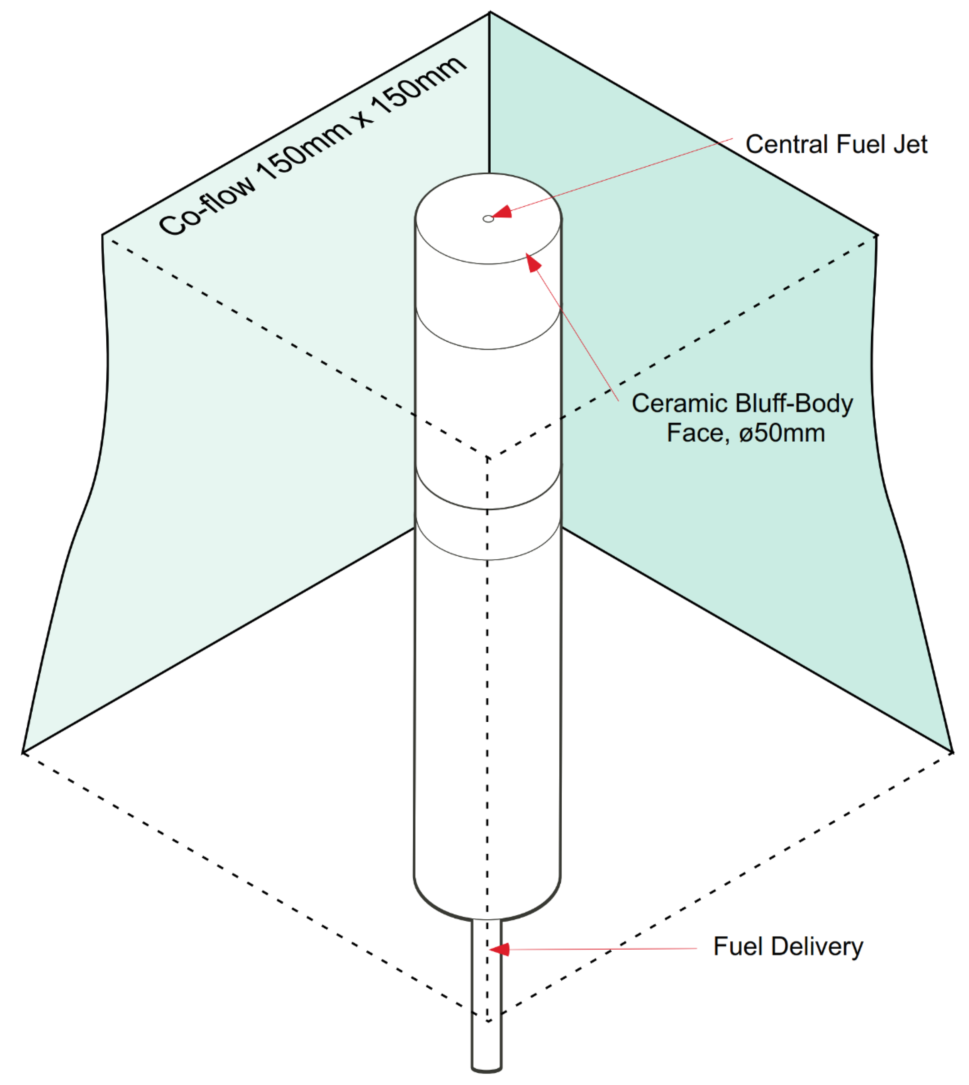
Figure 2.
Photo of an HM (CH4 ⁄ H2) flame. Source: School of Aerospace, Mechanical and Mechatronic Engineering (AMME) at the University of Sydney, Australia (used with courteous permission).
Figure 2.
Photo of an HM (CH4 ⁄ H2) flame. Source: School of Aerospace, Mechanical and Mechatronic Engineering (AMME) at the University of Sydney, Australia (used with courteous permission).
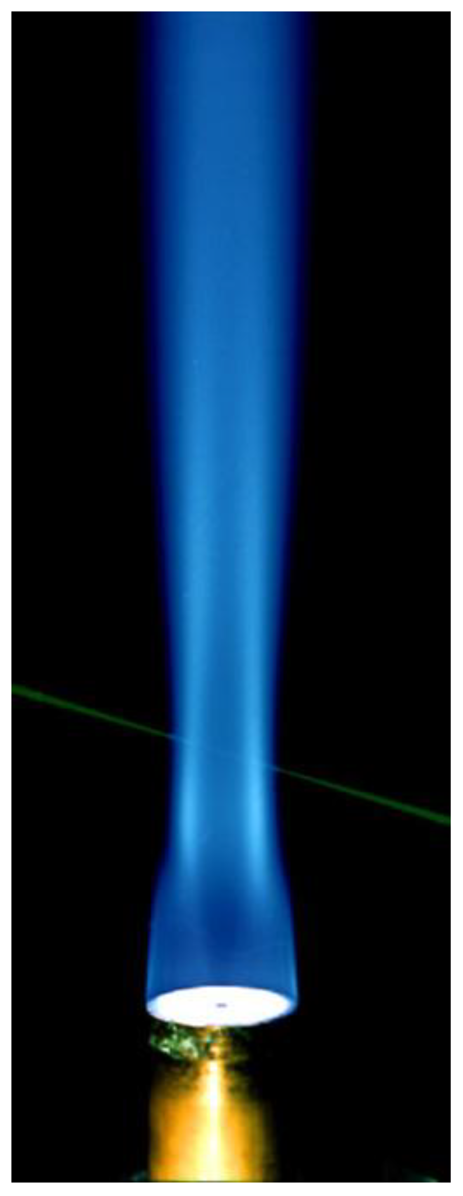
Figure 3.
Illustration of the blocks and inlet streams in the computational domain.
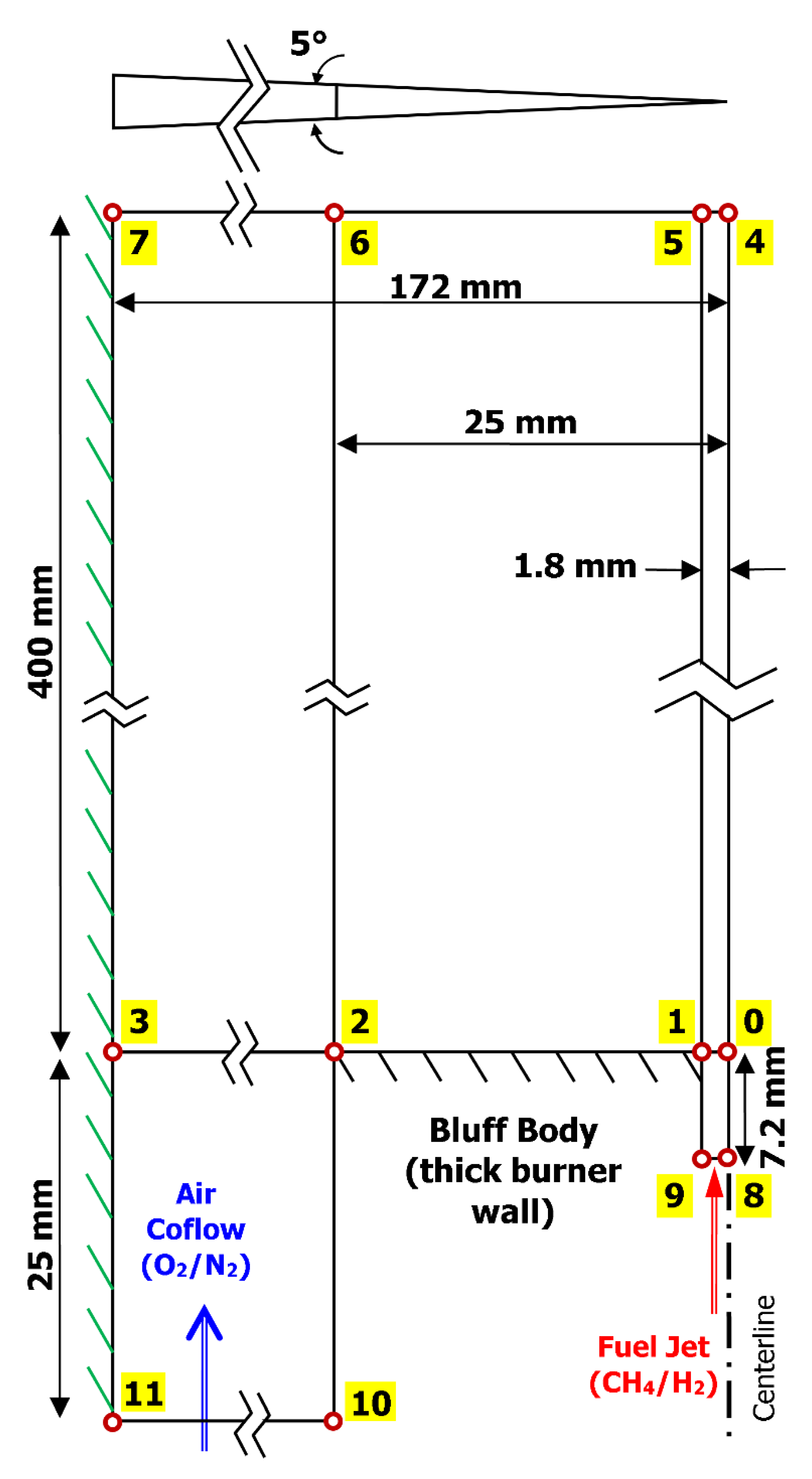
Figure 4.
Axial velocity at an axial distance of 5 mm (0.1 × burner diameter).
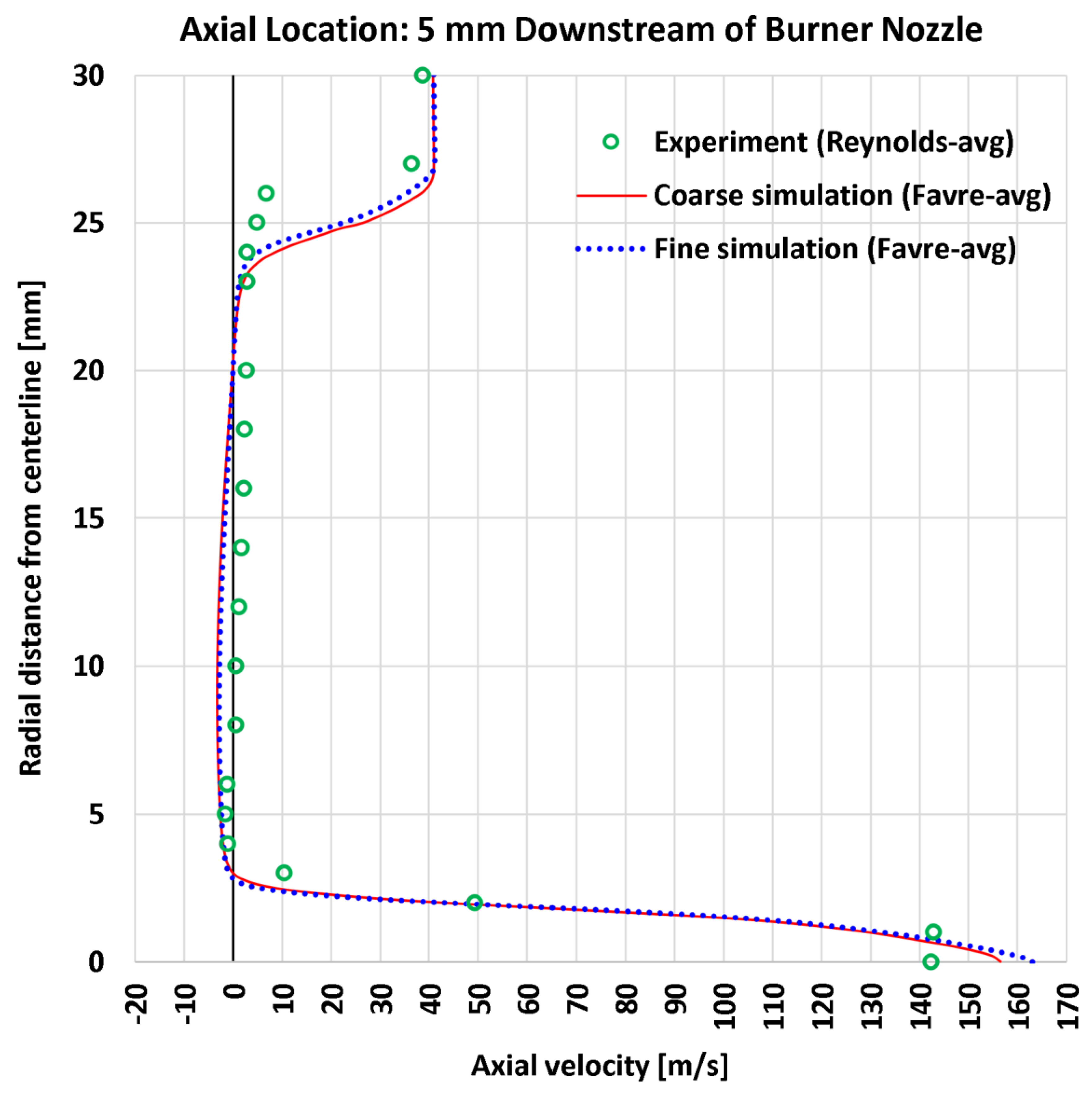
Figure 5.
Axial velocity at an axial distance of 13 mm (0.26 × burner diameter).
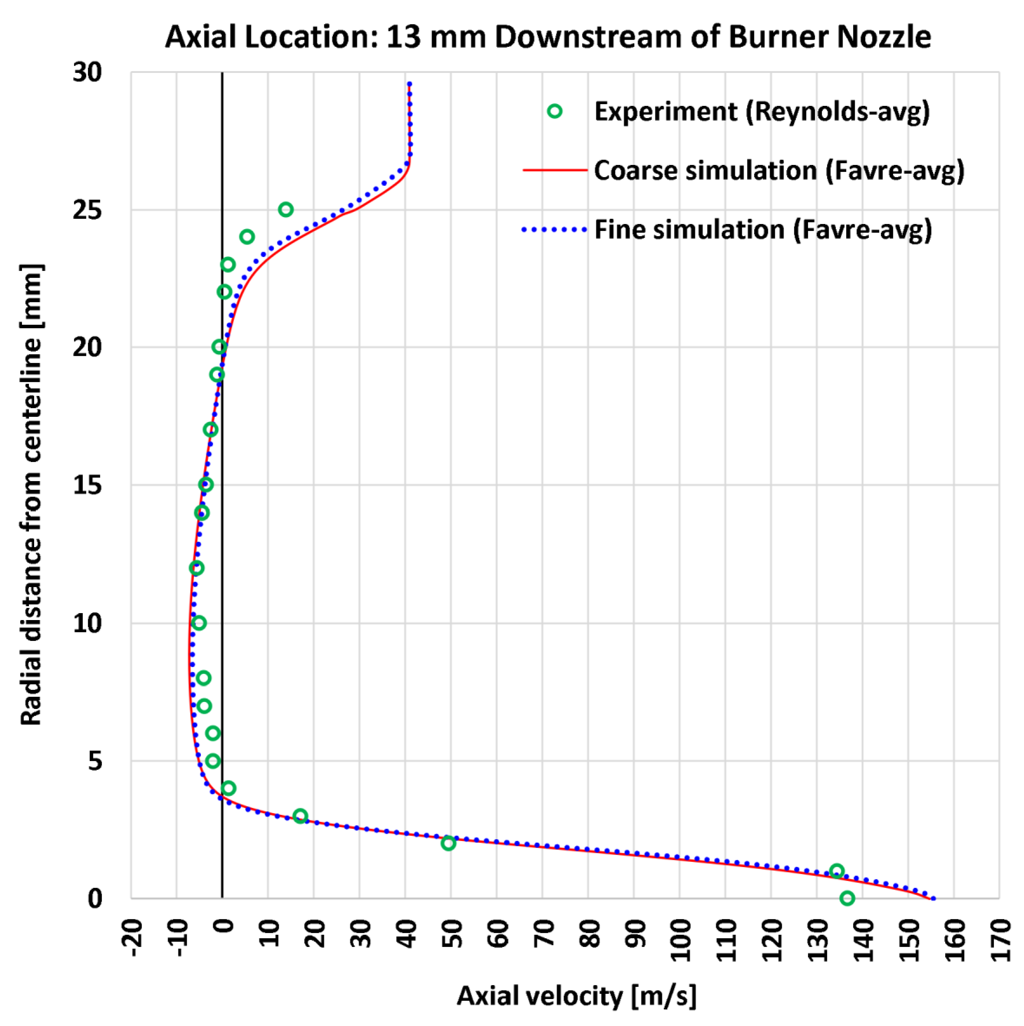
Figure 6.
Axial velocity at an axial distance of 30 mm (0.6 × burner diameter).
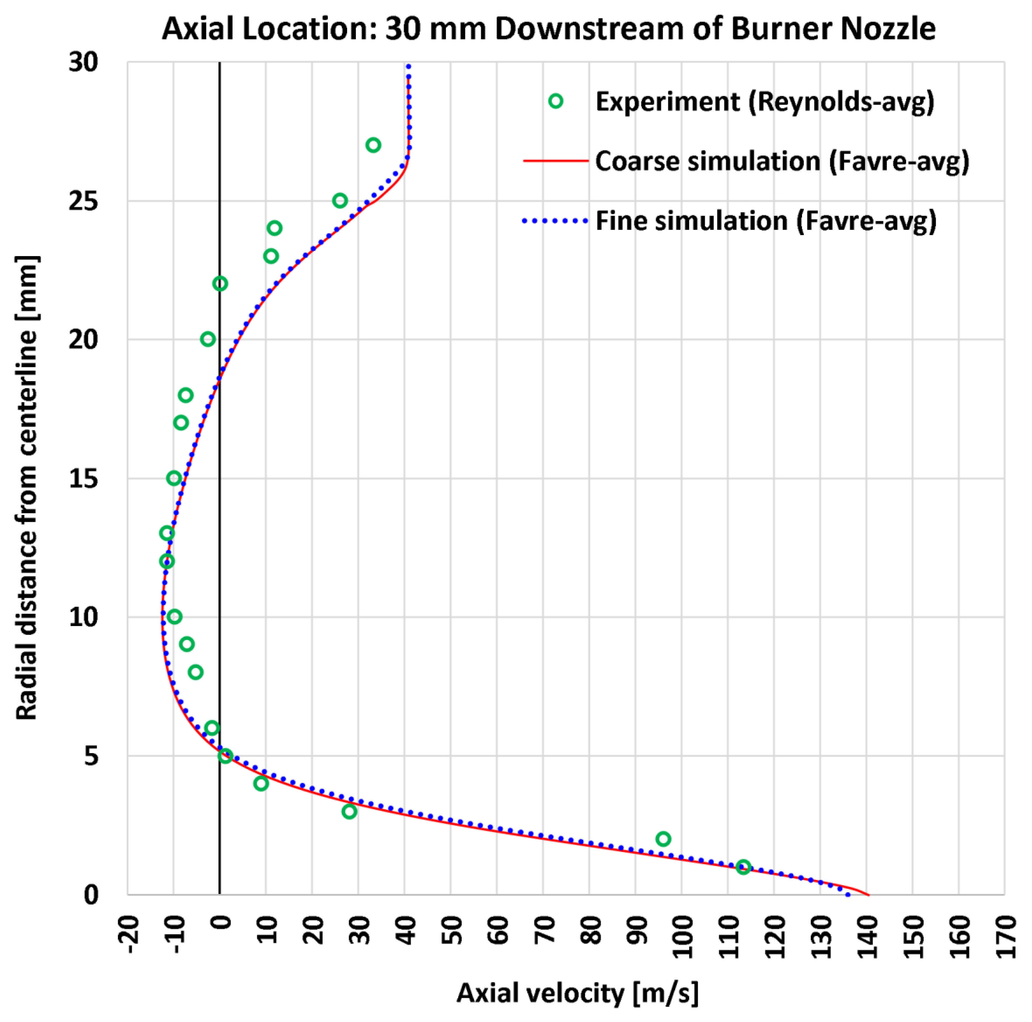
Figure 7.
Axial velocity at an axial distance of 45 mm (0.9 × burner diameter).
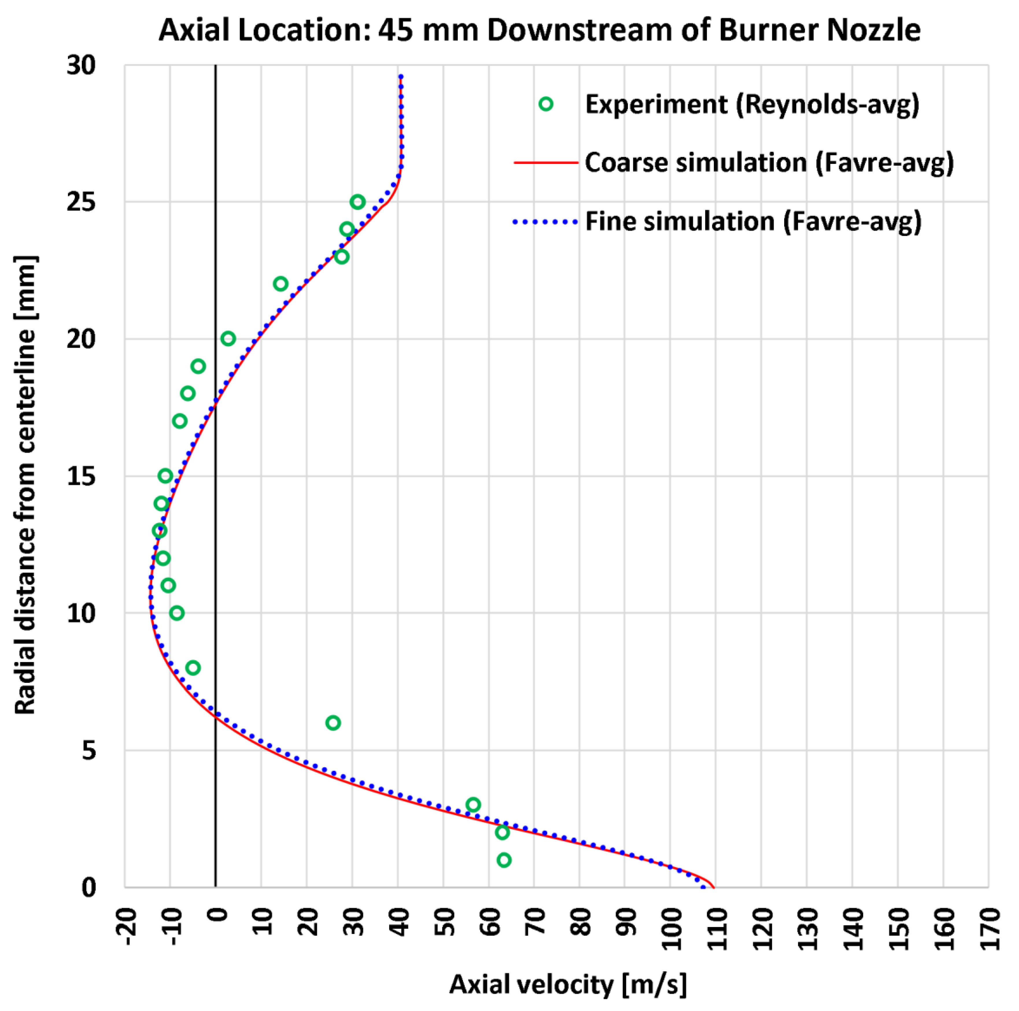
Figure 8.
Axial velocity at an axial distance of 65 mm (1.3 × burner diameters).
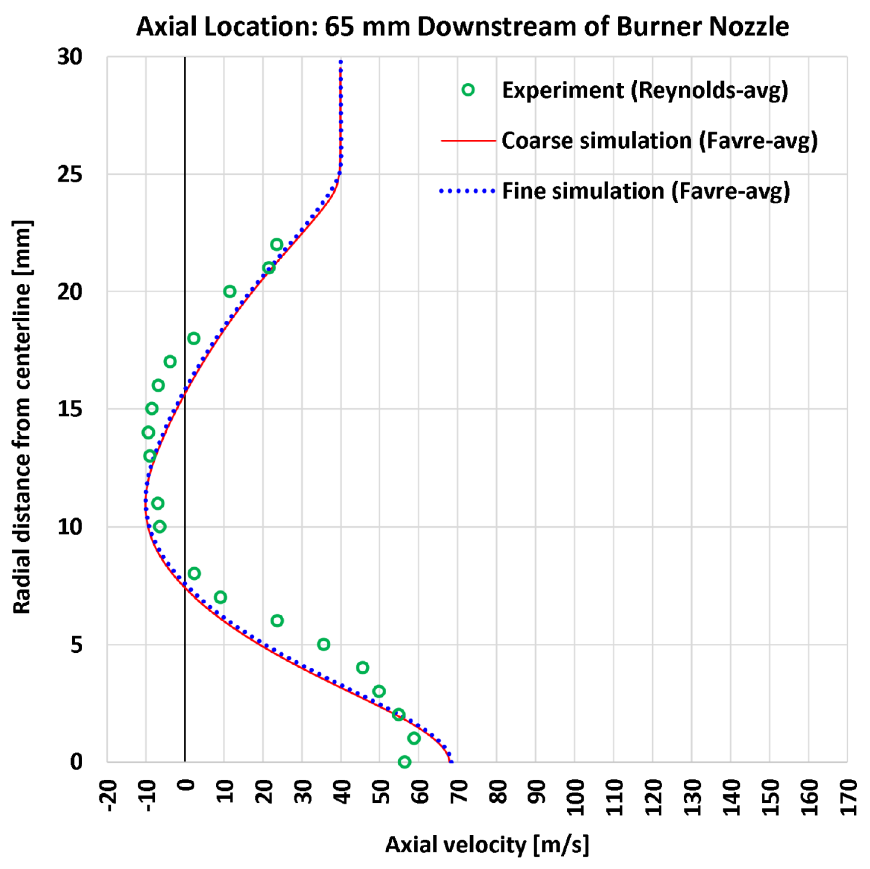
Figure 9.
Radial velocity at an axial distance of 5 mm (0.1 × burner diameter).
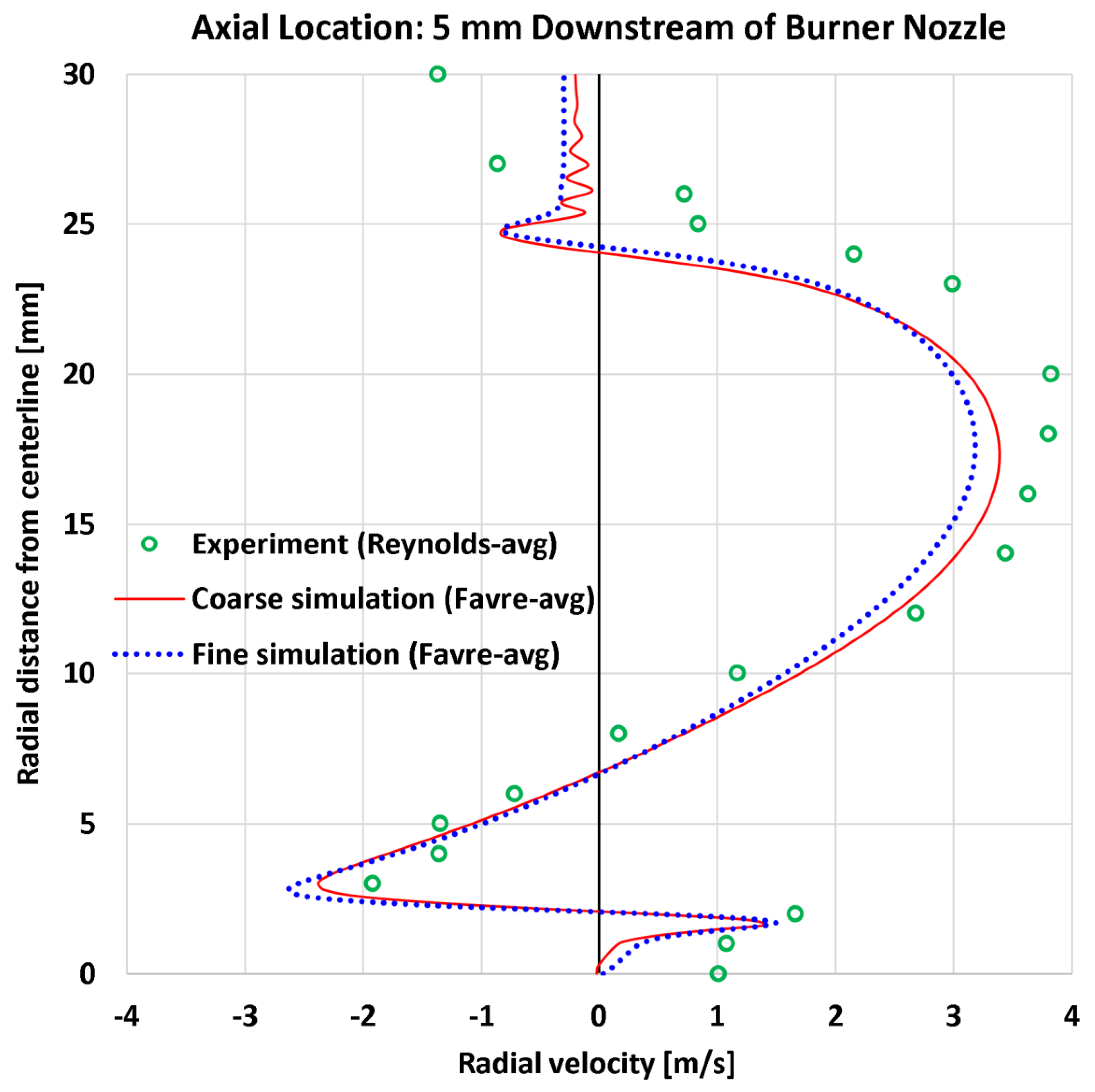
Figure 10.
Radial velocity at an axial distance of 13 mm (0.26 × burner diameter).
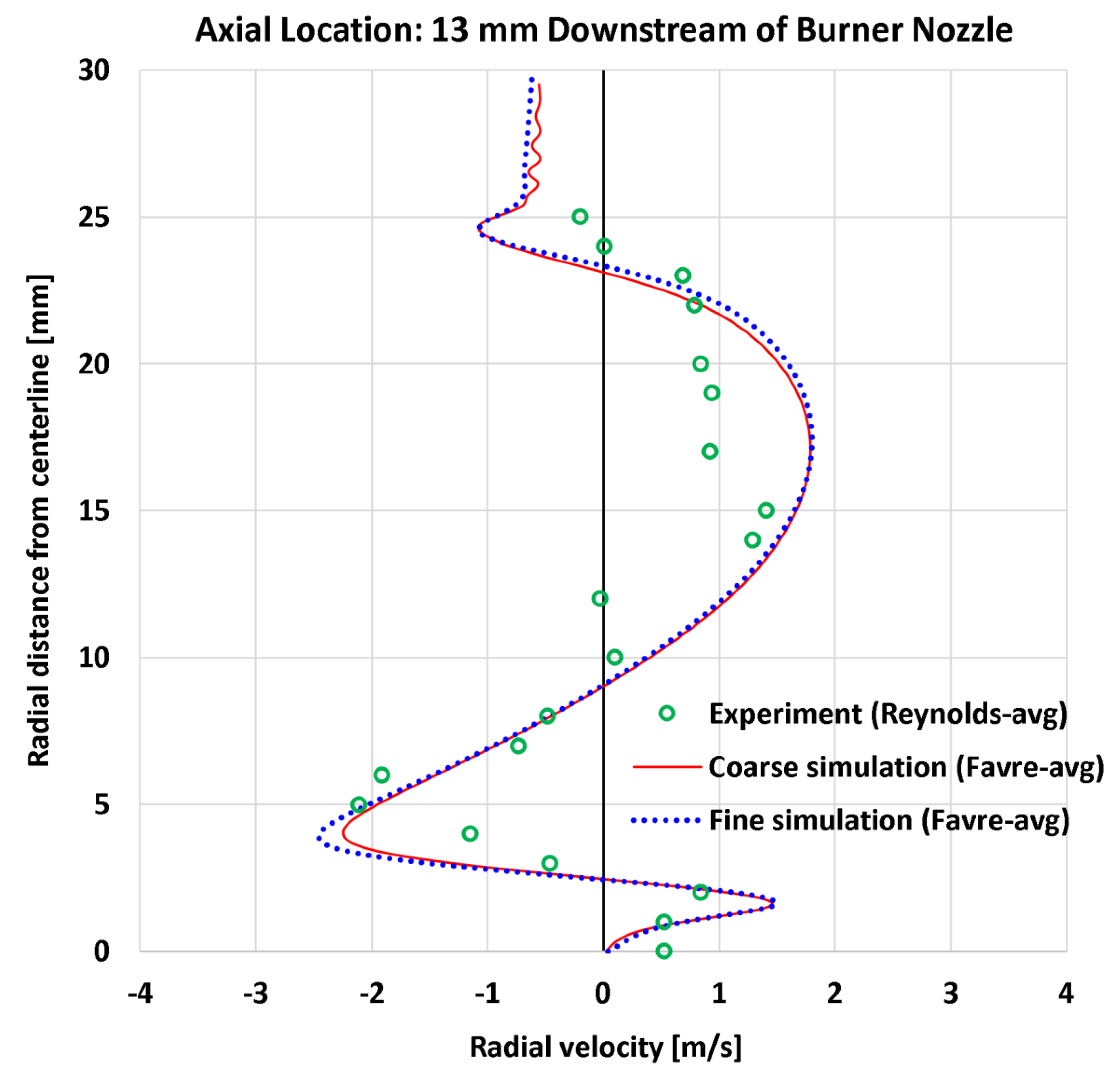
Figure 11.
Radial velocity at an axial distance of 30 mm (0.6 × burner diameter).
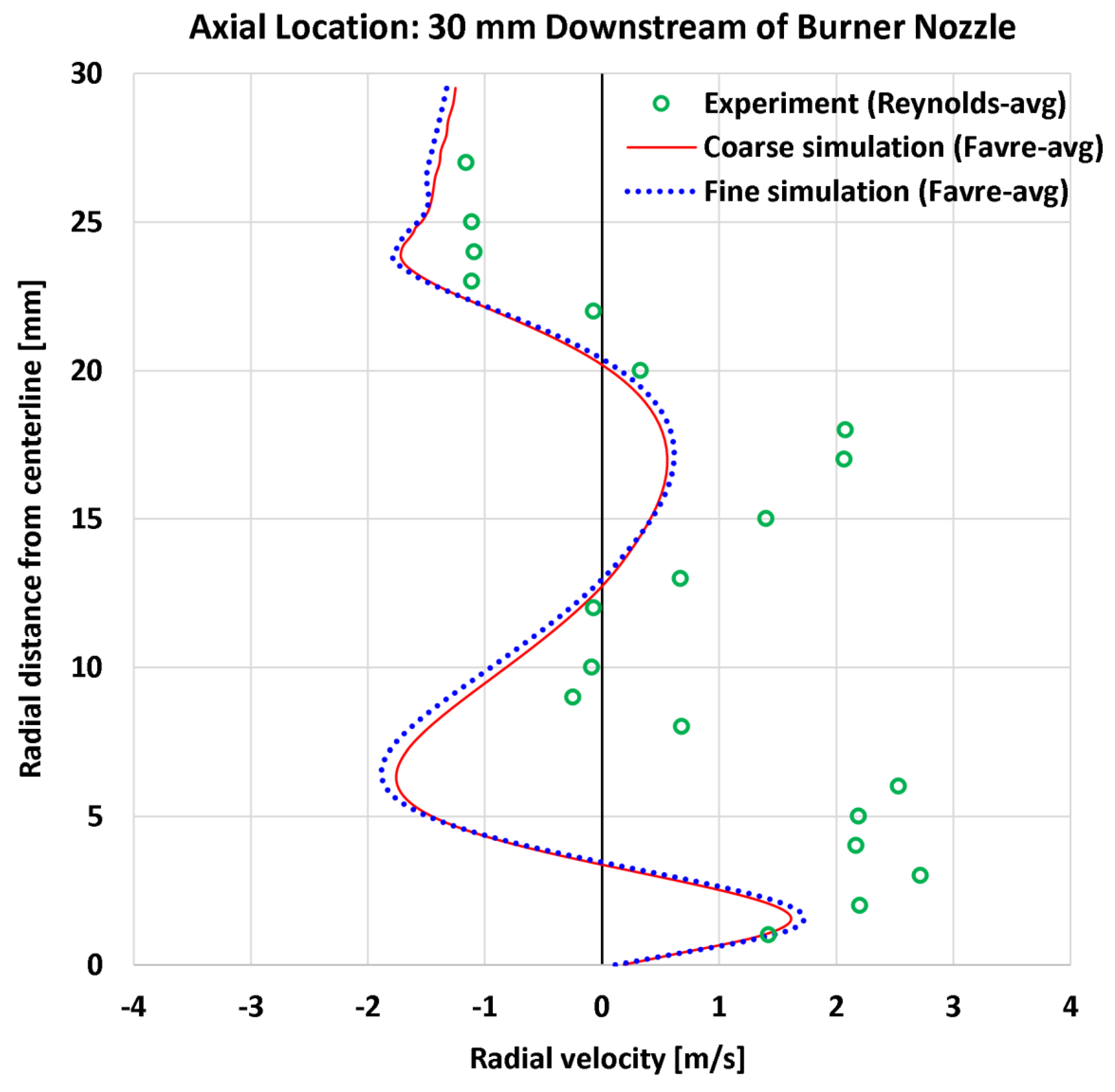
Figure 12.
Radial velocity at an axial distance of 45 mm (0.9 × burner diameter).
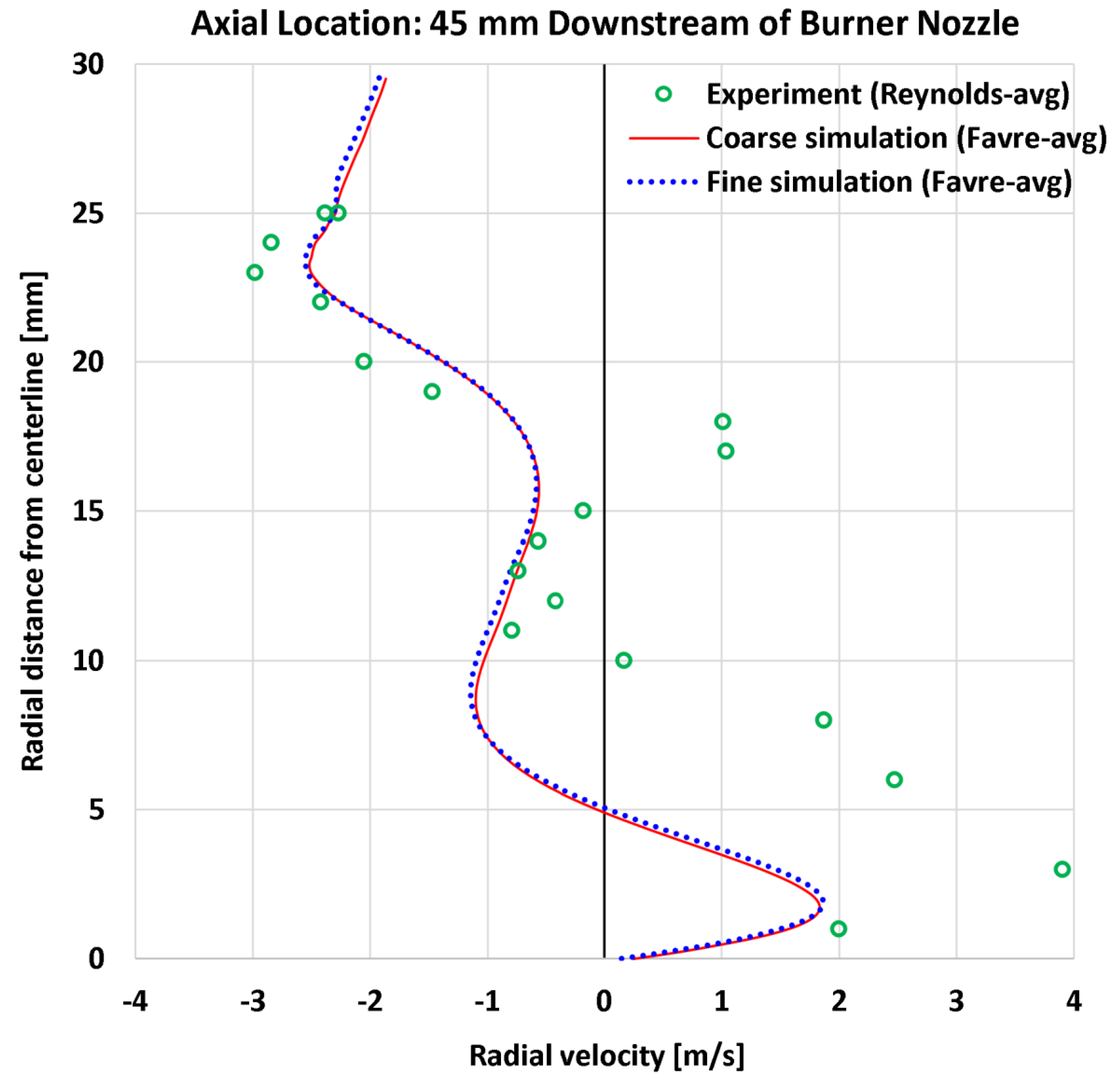
Figure 13.
Radial velocity at an axial distance of 65 mm (1.3 × burner diameters).
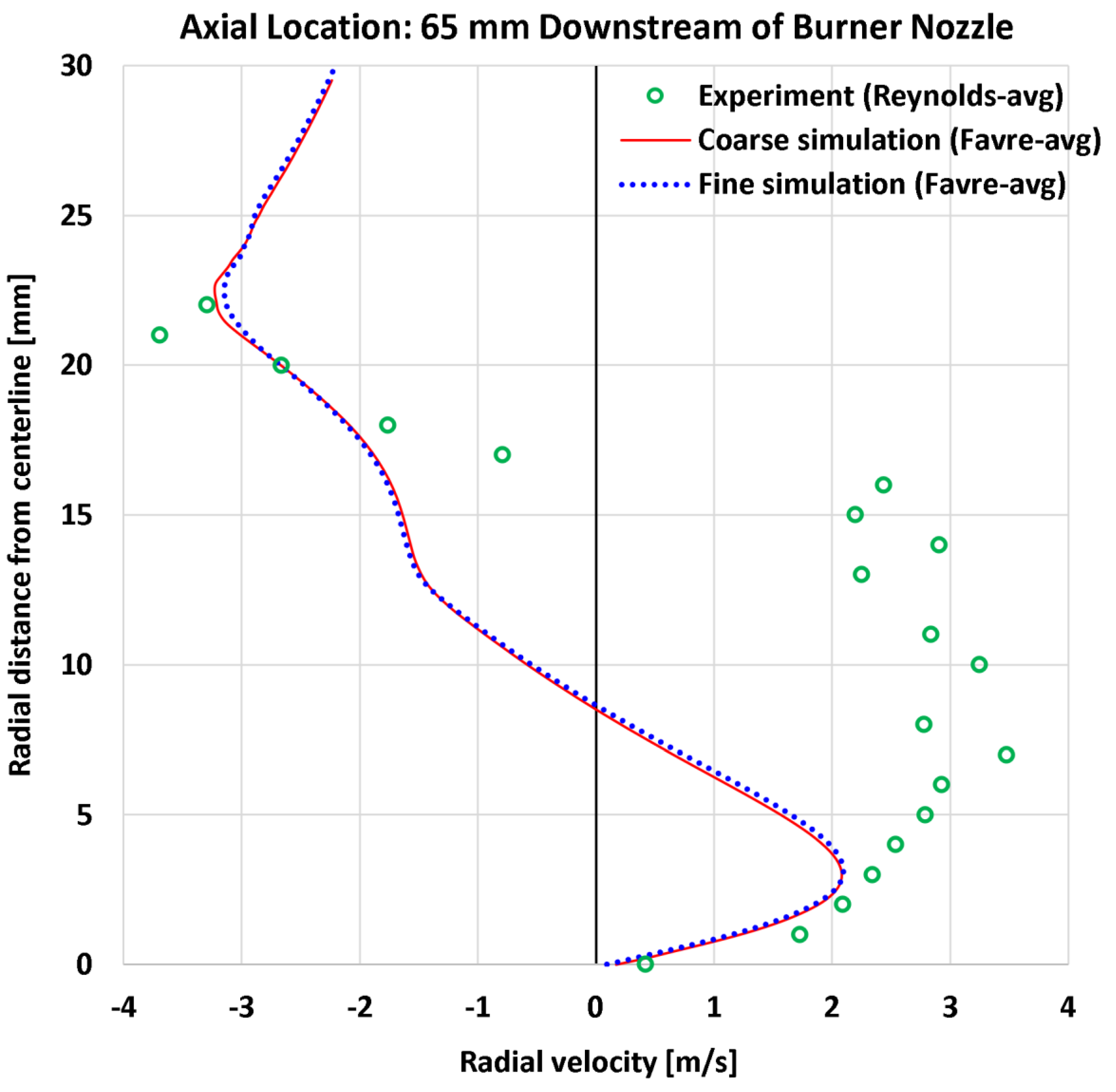
Figure 14.
Mass fraction of CH4 at an axial distance of 13 mm (0.26 × burner diameter).
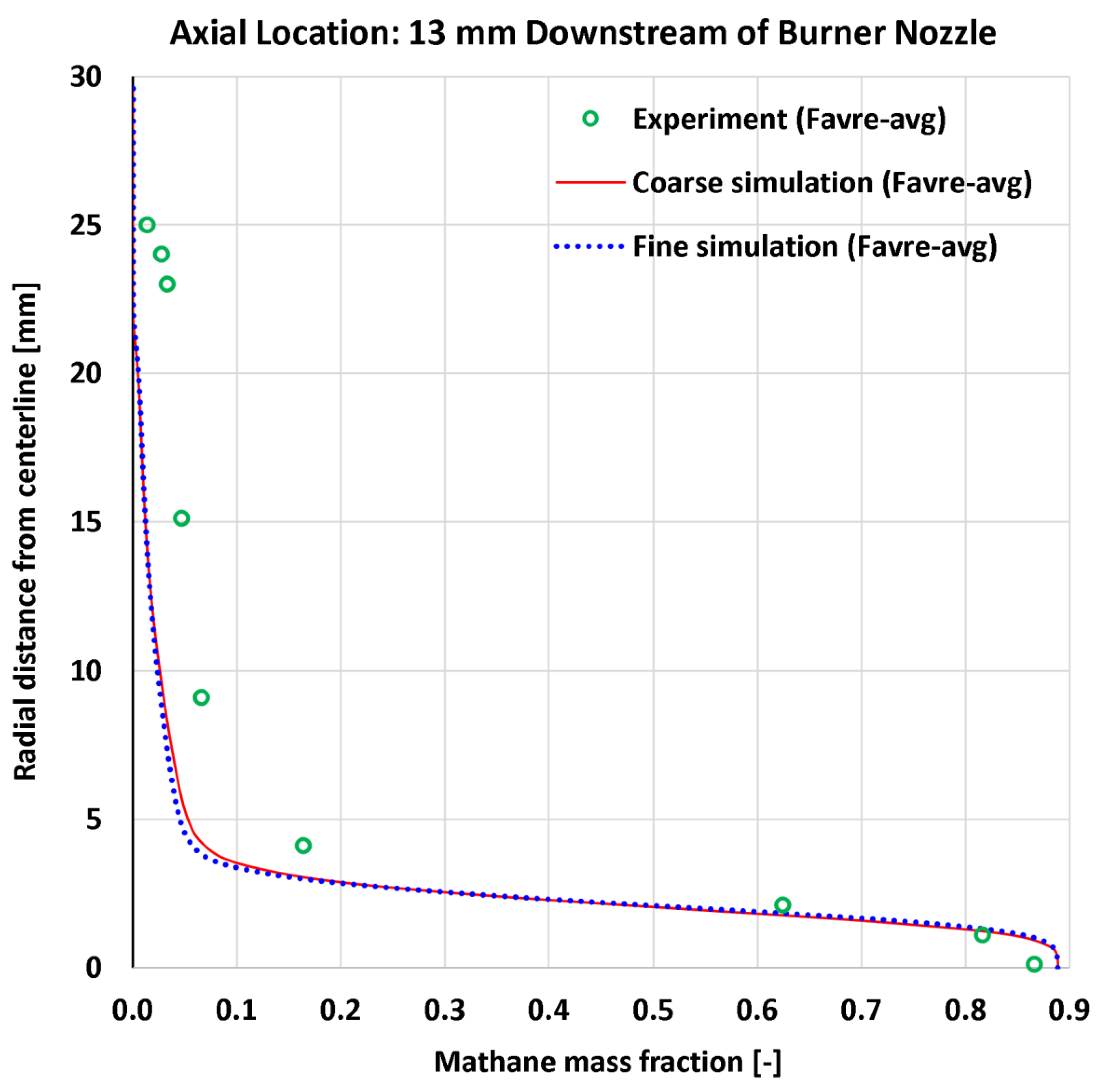
Figure 15.
Mass fraction of CH4 at an axial distance of 30 mm (0.60 × burner diameter).
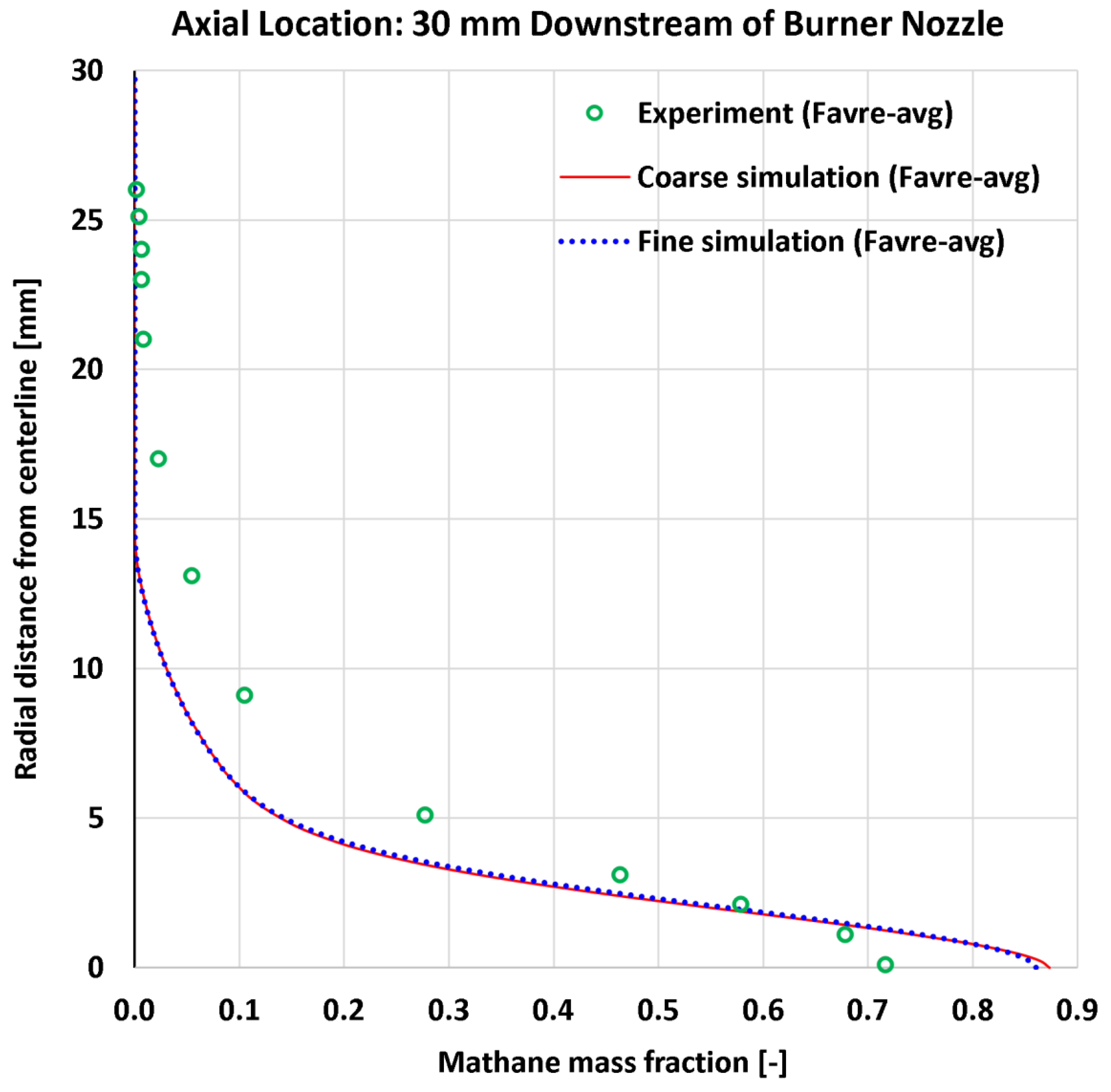
Figure 16.
Mass fraction of H2O at an axial distance of 13 mm (0.26 × burner diameter).
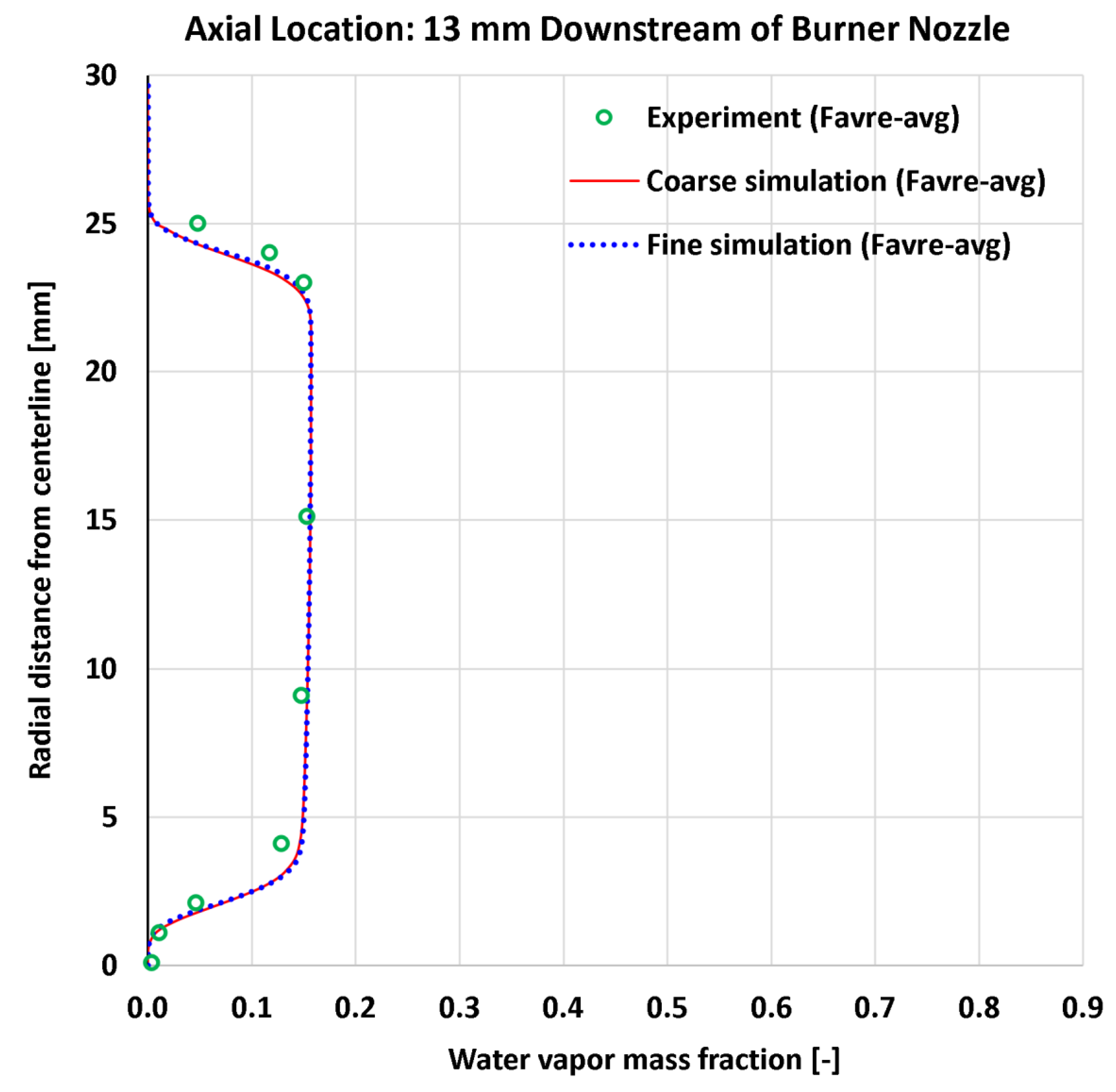
Figure 17.
Mass fraction of H2O at an axial distance of 30 mm (0.60 × burner diameter).
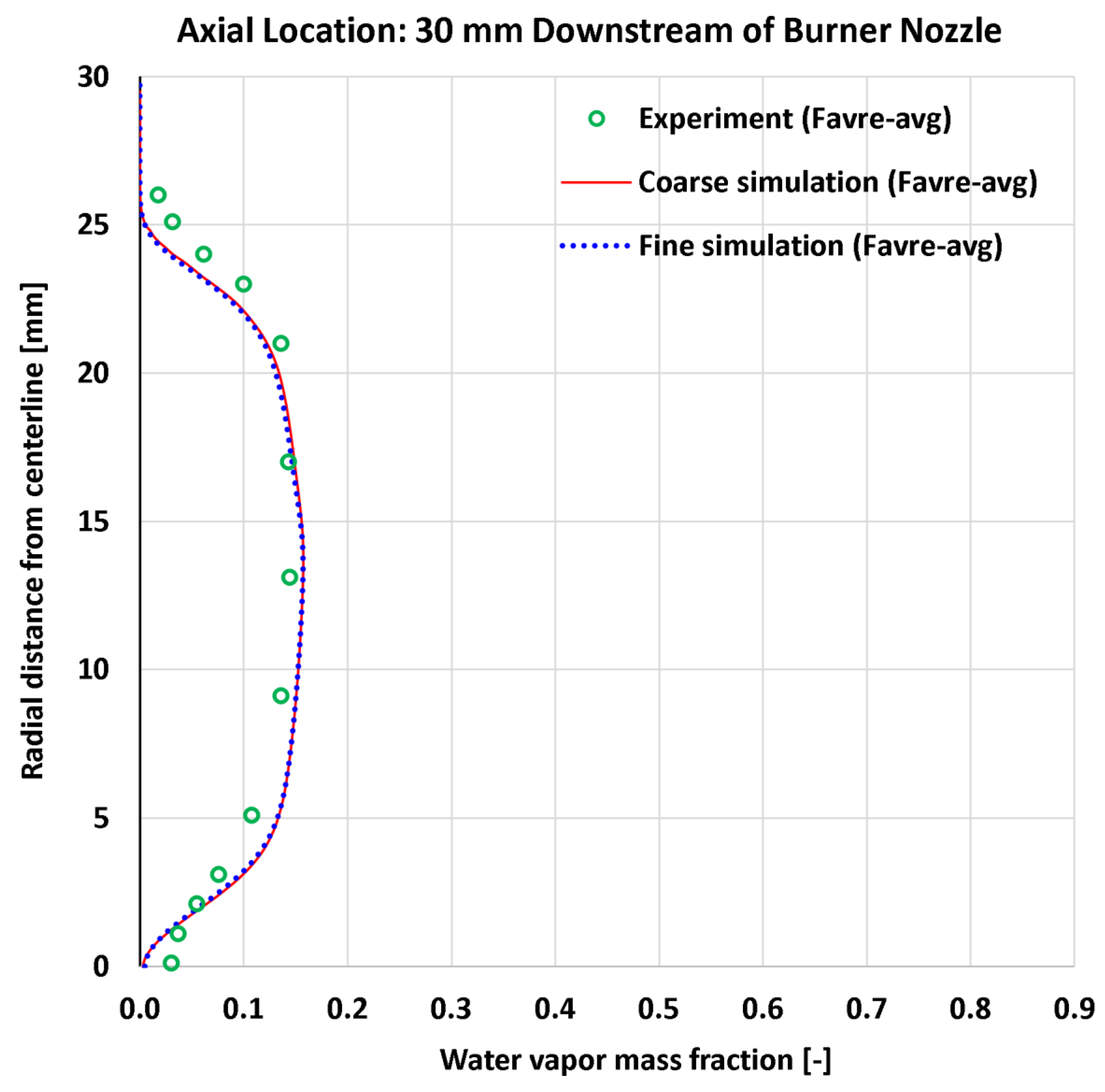
Figure 18.
Near-centerline mass fraction of CH4 (0.022 × burner diameter from centerline).
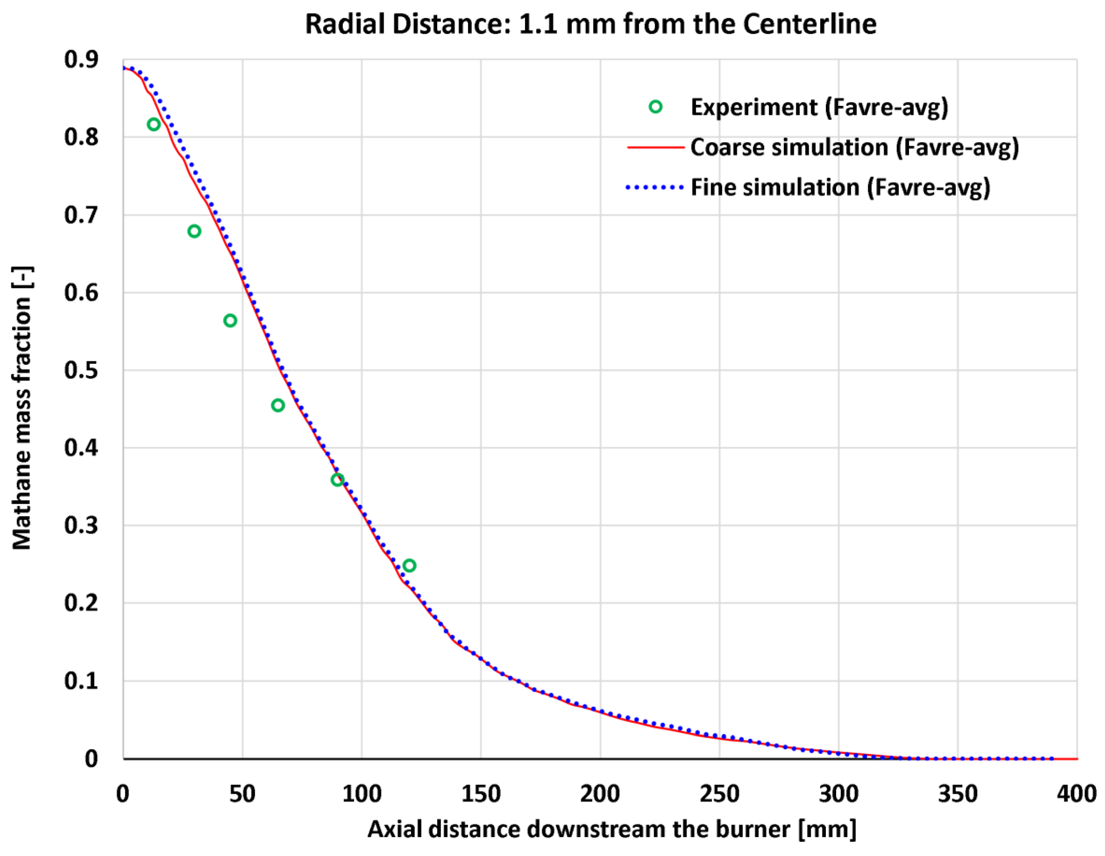
Figure 19.
Near-centerline mass fraction of H2O (0.022 × burner diameter from centerline).
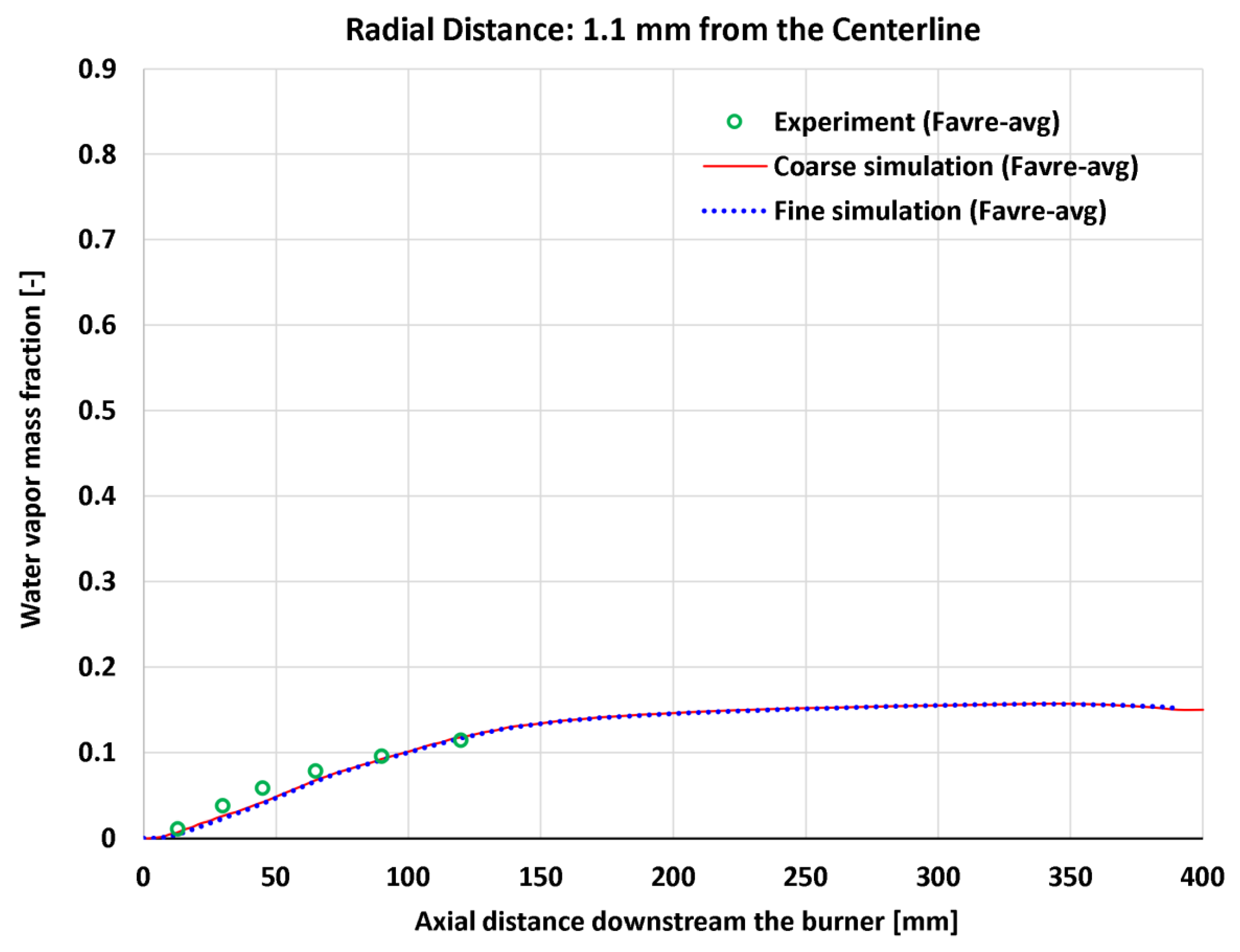
Figure 20.
Near-centerline temperature (0.022 × burner diameter from centerline).
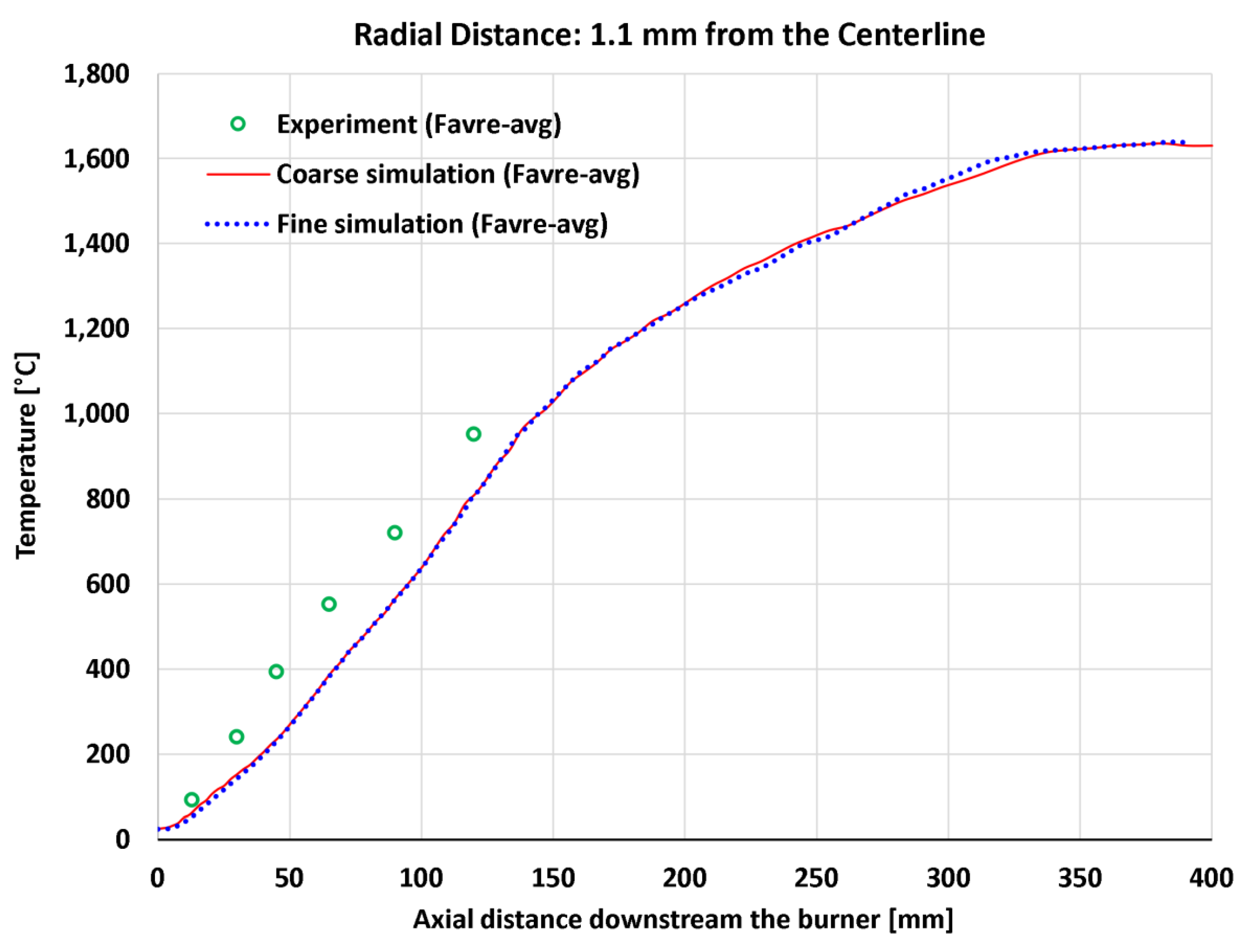

Table 1.
Reported characteristics of the experimental HM1 flame (experiment B4F3).
| Wind tunnel dimensions | 305 × 305 mm |
| Fuel jet diameter | 3.6 mm |
| Bluff-body diameter | 50 mm |
| Fuel jet mixture | CH4/H2 (1:1 or 50/50% by mole) |
| Fuel jet speed | 118.0 m/s |
| Blow-off speed | 235.0 m/s |
| %Blow-off (fuel jet speed ÷ blow-off speed) | 50.2% |
| Coflow air velocity | 40 m/s |
| Coflow turbulence intensity | 2% |
| Mass fraction of O2 in the coflow | 0.233 (21% by mole) |
| Mass fraction of N2 in the coflow | 0.767 (79% by mole) |
| Reynolds number of the fuel jet | 15,800 |
| Temperature of the fuel jet at the exit nozzle | 298 K |
| Momentum flux of the fuel jet | 0.03370 N |
| Adiabatic flame temperature | 2,265 K |
| Year of the experiment | 1995 |
Table 2.
Absolute quantitative measures of the deviations between the presented experimental profiles and computational profiles.
Table 2.
Absolute quantitative measures of the deviations between the presented experimental profiles and computational profiles.
| Index | Profile Type | HM1 Variable | Number of Points | Unit | MAD | RMS | ||
| Coarse | Fine | Coarse | Fine | |||||
| 1 | Radial | Axial velocity at 5 mm | 20 | m/s | 7.06 | 6.54 | 10.41 | 9.80 |
| 2 | Radial | Axial velocity at 13 mm | 22 | m/s | 5.11 | 4.66 | 7.11 | 6.79 |
| 3 | Radial | Axial velocity at 30 mm | 21 | m/s | 6.16 | 5.99 | 8.31 | 7.91 |
| 4 | Radial | Axial velocity at 45 mm | 22 | m/s | 6.88 | 6.48 | 9.94 | 9.60 |
| 5 | Radial | Axial velocity at 65 mm | 24 | m/s | 6.16 | 5.57 | 7.56 | 6.90 |
| 6 | Radial | Radial velocity at 5 mm | 20 | m/s | 0.77 | 0.78 | 0.91 | 0.87 |
| 7 | Radial | Radial velocity at 13 mm | 22 | m/s | 0.53 | 0.54 | 0.63 | 0.65 |
| 8 | Radial | Radial velocity at 30 mm | 21 | m/s | 1.23 | 1.24 | 1.68 | 1.70 |
| 9 | Radial | Radial velocity at 45 mm | 22 | m/s | 0.94 | 0.94 | 1.39 | 1.37 |
| 10 | Radial | Radial velocity at 65 mm | 24 | m/s | 1.58 | 1.58 | 2.22 | 2.21 |
| 11 | Radial | CH4 mass fraction at 13 mm | 9 | - | 0.04850 | 0.04985 | 0.06283 | 0.06255 |
| 12 | Radial | CH4 mass fraction at 30 mm | 13 | - | 0.05462 | 0.05199 | 0.07626 | 0.07223 |
| 13 | Radial | H2O mass fraction at 13 mm | 9 | - | 0.01759 | 0.01668 | 0.02342 | 0.02206 |
| 14 | Radial | H2O mass fraction at 30 mm | 13 | - | 0.01895 | 0.01896 | 0.02065 | 0.02104 |
| 15 | Axial | CH4 mass fraction at 1.1 mm | 6 | - | 0.04359 | 0.05175 | 0.05079 | 0.05941 |
| 16 | Axial | H2O mass fraction at 1.1 mm | 6 | - | 0.00792 | 0.00937 | 0.00934 | 0.01088 |
| 17 | Axial | Temperature at 1.1 mm | 6 | °C | 123 | 127 | 133 | 136 |
Table 3.
Relative quantitative measures of the deviations between the presented experimental profiles and computational profiles.
Table 3.
Relative quantitative measures of the deviations between the presented experimental profiles and computational profiles.
| Index | Profile Type | HM1 Variable | Maximum (Experimental) | Unit | %MAD | %RMS | ||
| Coarse | Fine | Coarse | Fine | |||||
| 1 | Radial | Axial velocity at 5 mm | 142.95 | m/s | 4.939% | 4.575% | 7.282% | 6.857% |
| 2 | Radial | Axial velocity at 13 mm | 136.84 | m/s | 3.731% | 3.404% | 5.198% | 4.960% |
| 3 | Radial | Axial velocity at 30 mm | 113.51 | m/s | 5.426% | 5.275% | 7.320% | 6.969% |
| 4 | Radial | Axial velocity at 45 mm | 63.54 | m/s | 10.821% | 10.203% | 15.637% | 15.111% |
| 5 | Radial | Axial velocity at 65 mm | 58.90 | m/s | 10.456% | 9.462% | 12.832% | 11.723% |
| 6 | Radial | Radial velocity at 5 mm | 3.82 | m/s | 20.19% | 23.73% | 20.37% | 22.69% |
| 7 | Radial | Radial velocity at 13 mm | 1.41 | m/s | 37.93% | 38.39% | 44.70% | 45.89% |
| 8 | Radial | Radial velocity at 30 mm | 2.72 | m/s | 45.15% | 45.58% | 61.93% | 62.36% |
| 9 | Radial | Radial velocity at 45 mm | 4.70 | m/s | 20.07% | 20.07% | 29.53% | 29.21% |
| 10 | Radial | Radial velocity at 65 mm | 3.48 | m/s | 45.44% | 45.33% | 63.66% | 63.47% |
| 11 | Radial | CH4 mass fraction at 13 mm | 0.86616 | - | 5.600% | 5.756% | 7.254% | 7.222% |
| 12 | Radial | CH4 mass fraction at 30 mm | 0.71701 | - | 7.618% | 7.251% | 10.636% | 10.073% |
| 13 | Radial | H2O mass fraction at 13 mm | 0.15302 | - | 11.497% | 10.900% | 15.307% | 14.418% |
| 14 | Radial | H2O mass fraction at 30 mm | 0.14422 | - | 13.138% | 13.149% | 14.321% | 14.592% |
| 15 | Axial | CH4 mass fraction at 1.1 mm | 0.81633 | - | 5.339% | 6.339% | 6.221% | 7.278% |
| 16 | Axial | H2O mass fraction at 1.1 mm | 0.11439 | - | 6.925% | 8.188% | 8.165% | 9.514% |
| 17 | Axial | Temperature at 1.1 mm | 1,224 | °C | 10.051% | 10.413% | 10.828% | 11.088% |
| Average for 12 profiles (excluding the five radial velocity profiles ) | 7.962% | 7.910% | 10.083% | 9.984% | ||||
Disclaimer/Publisher’s Note: The statements, opinions and data contained in all publications are solely those of the individual author(s) and contributor(s) and not of MDPI and/or the editor(s). MDPI and/or the editor(s) disclaim responsibility for any injury to people or property resulting from any ideas, methods, instructions or products referred to in the content. |
© 2025 by the authors. Licensee MDPI, Basel, Switzerland. This article is an open access article distributed under the terms and conditions of the Creative Commons Attribution (CC BY) license (http://creativecommons.org/licenses/by/4.0/).
Copyright: This open access article is published under a Creative Commons CC BY 4.0 license, which permit the free download, distribution, and reuse, provided that the author and preprint are cited in any reuse.


