
Submitted:
14 January 2026
Posted:
15 January 2026
You are already at the latest version
Abstract
The objective of this work is to propose a simulation strategy for production planning that is compatible with the dynamism of natural gas processing, especially under open-market arrangement, in which several scheduling simulations must be performed within short time horizons. In such contexts, traditional first-principles-based ap-proaches, although accurate, require prohibitive computational times, motivating the need for an alternative simulation strategy. This work thus proposes a data-driven model built with the aid of machine learning and applied in a case study with historical data from the largest gas processing site in Brazil: Cabiúnas Petrobras asset. Main plant flowrates were selected: 18 targets and 44 input candidates – 1282 observations from three and a half years of operation. Principal Component Analysis was used for order reduction, keeping the 22 main principal components. A forward neural network (2 hidden layers and 225 neurons per layer) was built from training/test sets randomly selected and optimized hyperparameters – learning rate (0.001533) and batch size (8). Training converged in roughly 200 epochs (Adam optimizer), with early stop triggered by validation set. A mean absolute error of 0.0017 (test set) and R2=0.72 were found, a promising result considering plant complexity and data simplicity. Results showed particularly good fit for lighter products (sales gas, natural gas liquid), also indicating an opportunity for further work by including inputs related to liquid fractionation.
Keywords:
natural gas
; machine learning
; deep neural network
; process simulation
1. Introduction
A key step of the Oil & Gas chain is midstream natural gas processing, necessary to give destination to the associated natural gas and ensure market-specification for end use [1]. This area is characterized by the dynamic operation scenarios as it needs to adapt to upstream and downstream varying conditions. Those changes translate into several scheduling and production planning prediction scenarios that are daily reviewed with newer information for better decision making. This is especially relevant in the context of the Brazilian gas market, where recent regulatory changes yielded an open market arrangement in which third parties can access the natural gas processing infrastructure such as Petrobras’ [2].
In this new dynamic, the gas processor provides a gas processing service for the third-party companies [3]. As a result, several additional production planning processes were created to account for this fast-paced dynamic now involving multiple contracting parties [4]. In the Brazilian context, those new scheduling processes require now over a thousand process simulation scenarios per month, for each gas processing plant [4]. This scenario gets even more complex when the processing site receives raw gas from multiple feedstocks and is formed by multiple Natural Gas Processing Units (NGPUs) and Liquid Fractionation Units (LFUs) with distinguished layouts, technology and performance. The resulting flexibility of this site translates into multiple operation and configuration possibilities, which directly affects the product profile distribution for the same raw gas inputs [5].
A new simulation strategy is necessary to fulfill the requirements of those new processes: agility, reliability, robustness, auditability. The traditional first principles approach, however solid in theoretical basis, demands a high execution time, hampering industrial applications for the execution of multiple scenarios in a short time window availability. First principles simulation is the benchmark approach in this field, and Aspen HYSYS stands out as the market-leading commercial process simulator for natural gas processing [4,5]. This approach is capable of depicting the engineering phenomena underlying the process units. However, its drawbacks are: (1) the need of understanding and modelling all the phenomena and knowing all the parameters involved in it to both develop a new model and to update an existing one [6]; (2) the high simulation cost in terms of execution time for complex models. The latter is particularly relevant when several model evaluations are required, which is the case when (a) the simulation model is coupled with an optimization algorithm or (b) the simulation model is being used for multiple-scenario/case-study evaluations, which applies to this work.
In this context, recent works on modelling and optimization of a natural gas processing site proposed a business optimization framework coupled with a phenomenological modelling for an industrial site with multiple NGPUs and feedstock [3,4]. The methodology proposed led to promising results, however the total MINLP optimization time reached long 24 hours, mostly due to the high cost of first-principles model evaluation [4]. Industrial implementation requires a shorter execution time and therefore other modelling strategies should be investigated.
A promising approach is to explore machine learning techniques to develop data-driven and/or physics-informed machine learning models. This strategy tends to result in models that demand lower computation effort during usage – this shorter execution time might enable real-time simulation and therefore usage for optimization, control, RTO, digital twin and rigorous scheduling applications. Machine learning models are also particularly interesting for industrial applications because of their inherent capability for updating adherence to the real plant – the model parameters can be periodically updated from newly acquired plant data.
Machine learning has been employed in the oil and gas industry for generating models for use in optimization and control, among other applications. For example, Soares et al. (2022) [7] developed a nonlinear model predictive controller (NMPC) for a gas-lift system, in which the internal states were inferred from sensor data using a machine learning algorithm. The literature also presents studies in which machine learning has been applied in gas-oil systems for data-driven process modeling and for forecasting hydrocarbon production. For example, Chahar et al. (2022) and Fernandes et al. (2025) predicted well performance from historical production and reservoir data [8,9], and Han and Kwon (2021) applied deep learning models to shale gas wells [10]. However, the specific use of input-output flowrate modeling based on machine learning to forecast production in NPGUs has not been previously addressed, this study being the first contribution to the knowledge of the authors. To fill this gap, this work proposes a new simulation approach, compatible with the dynamism of the open-market midstream sector: a data-driven model built with the aid of machine learning and tested in an industrial case study at the largest gas processing site in Brazil: a Petrobras asset.
2. Materials and Methods
To achieve the objective of this work, a practical case study will be used to test the proposed strategy and the resulting data-driven model in an actual industrial plant. The selected site is owned by Petrobras and is the largest natural gas processing plant in Brazil – Cabiúnas Gas Plant (UTGCAB), located in Macaé, Rio de Janeiro.
Information on UTGCAB operation history was collected, analyzed and used as data source to develop a data-driven model to predict the output production flowrates based on plant data at the same instant of time.
2.1. System Description
UTGCAB is part of the integrated natural gas processing system of the southeast of Brazil (Figure 1) [4]. It is a multi-unit and multi-feedstock gas processing asset that receives raw natural from both Santos and Campos Basin and processes the gas into four products: sales gas, NGL (natural gas liquid), LPG (liquified petroleum gas) and C5+ (natural gasoline). As shown in Figure 1, UTGCAB has 5 NGPUs and 3 LFUs, as well as specific units for contaminant removal (mercury and CO2). It also contains auxiliary systems for compression and multiple possibilities of gas and liquid routing from the slug catcher to the process units, along with several operation configuration for each processing unit, which translates into a challenge when trying to predict the output products flowrates.
2.2. Modeling Approach
When it comes to designing and operating process facilities in the Oil & Gas industry, having a digital essential for a wide range of technical evaluations and decision making, such as debottlenecking, technical support, logistics planning, optimization and process design [1]. However, to achieve that it is necessary to have readily-available, accurate, fast and updatable process models – and that is where the challenge remains.
To address this, a deep neural network (DNN) was adopted as the core modeling strategy. DNNs are well recognized for their strong performance in complex nonlinear regression tasks, due to their capacity as universal function approximators and their ability to model intricate patterns from large-scale, high-dimensional data [11,12,13]. Additionally, DNNs have become a widely adopted tool in scientific and engineering applications, supported by a robust body of theoretical research and practical successes. These characteristics make them particularly well-suited for process modeling tasks where both flexibility and accuracy are required. The network architecture, training strategy, and validation procedures are detailed in the following sections.
2.3. Problem Formulation
The formulated problem is a nonlinear steady-state model with the goal of predicting the flowrates of each plant product: sales gas, NGL, LPG and C5+. Both input and output variables are quantitative and continuous and are used in the same instant of time, without any lag.
There are 44 feature candidates, broken down in (1) raw gas and condensate flowrates from the outlet of the slug catchers to their respective destinations, (2) input gas flowrates of each NGPU, (3) flare and residual gas, (4) NGL flowrate to the LFUs. 18 targets were defined, which are the outlet flowrates of each product, from each process unit (NGPUs and LFUs).
A Forward Neural Network (FNN) framework was used. Even though the dataset used is strictly a time-series, the goal in this work is to come up with a neural network to model the process of natural gas processing. This means that the neural network must be able to provide an output at any given time from a set of inputs at this same time, regardless of that happened in the past. Therefore, this dataset is considered a series of independent observations in steady state, which explains the random selection of train/test data and the use of FNNs.
For the input layer, a linear activation function was used, whereas all other layers used ReLu [11]. The input layer has the size of the reduced training set, i.e., 22, whereas the output layer has the size of y, 18. Adam [14] was selected as the optimizer and the mean squared error (MSE), Equation 1, was used as loss function during training:
MSE is one of the most common metrics for regression models and computes the squared error between the actual target values (y) and the values predicted from the NN model (ypred).
A validation set of 20% was used during training to monitor the validation loss as a reference metric for Early Stopping, with a patience of 30 – the maximum number of epochs was set to 1000. Lastly, two regularization techniques were used: (a) Dropout was applied to each hidden layer, with a drop rate of 20%. (b) Elastic Net regularization (a combination of L1 and L2 techniques) was added to each layer with a default λ=0.01.
Due to the characteristics of deep learning, there is no general rule for selection of architecture and hyperparameters – although some rules of thumb could be used. In terms of architecture, the goal was to find the most concise neural network that returns a satisfactory output, in order to avoid the curse of dimensionality and overfitting. There are two main architecture parameters: (i) number of hidden layers and (ii) number of neurons per layer. The activation function and regularization techniques are also relevant here. There are still other parameters that affect neural network performance, for instance: (iii) learning rate and (iv) batch size.
In order to find the best neural network architecture within a certain parametric space, Optuna package was used for hyperparameter optimization. Parameters (i) to (iv) listed above were manipulated, according to Table 1, and the neural network was trained 500 times, with the objective of minimizing the loss function in the test set.
2.4. Process Dataset
Data selection was one of the most important steps in this work, since the quality of the resulting model will be restrained to the quality of the dataset utilized and, in this particular case, the data source comes from an industrial basis with all real-world complexity. The dataset chosen contains reconciled process history data of an industrial. plant for natural gas processing. This data is presented in a daily basis and consists of flowrate values measured/inferred at several distinguished locations in the plant. They represent the overall mass balance of the site and the local mass balance of each NGPU. A total of 1282 observations were selected for use, which describe three and a half years of plant operation, from January 2020 to June 2023.
2.5. Modeling Framework
All data analysis and modelling were executed in Python with keras API from tensorflow package. Auxiliary packages such as sklearn, numpy, pandas, matplotlib and seaborn were also used. Data analysis and storytelling were performed with the aid of (i) statistical descriptive analysis (mean, variance, standard variation), (ii) graphical plots (time-series trends, scatter plots, histograms), and (iii) unsupervised machine learning techniques. Principal component analysis (PCA) and clustering (hierarchical clustering and K-means) were the unsupervised machine learning methods utilized for data comprehension.
Then, a supervised-learning model was developed using deep neural networks, aiming to predict the outputs at a given instant t from the inputs at this same time.
3. Results and Discussion
3.1. ETL and Data Wrangling
The first steps carried out were data extraction/transformation/loading (ETL) and data wrangling, such as: header, index and variable type configuration, removal of time points with missing values and drop out of not useful variables. This procedure resulted in a clean and prepared dataset for feature/target selection.
From the original dataset, 44 variables were initially selected as features (X) and 18 as targets (y). After selecting the input variables from data history, those features were standardized by using the StandardScaler function from sklearn preprocessing package. This function returned the variables with zero mean and standard deviation equal to one, a pre-requisite to carry out PCA analysis. Train and test sets were then randomly determined from the original dataset with a test size of 20% – a typical reference from the literature. This resulted in 1025 observations for training and 257 for testing.
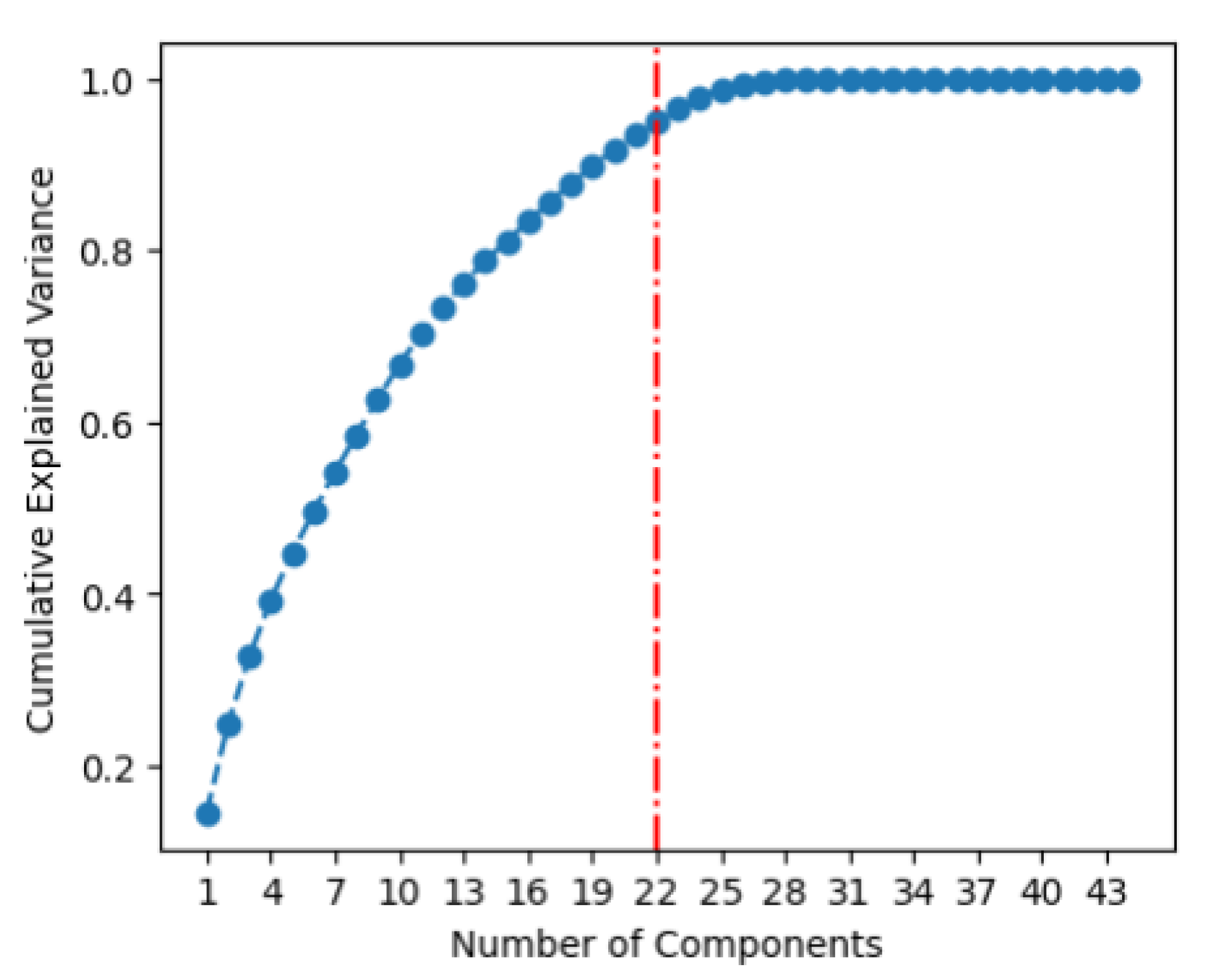
PCA analysis was carried out with the standardized input data. The training set was used to define the transformation space, which was then applied to the test set. The cumulative variance plot was used to help determine the number of components to keep, as seen in Figure 4. The chart shows the total amount of variance captured (y-axis) depending on the number of principal components included (x-axis). A general rule of thumb is to preserve around 80% of the variance – this is valid for the typical cases in which the first few components account for most of the variance. However, Figure 4 shows that for this dataset there is not a main feature that explains most of the variance. Data variance seems to be incrementally explained with the inclusion of new components for the first 29 principal components, which explain 100% of data variance. The last 15 components, then, seem to be redundant compared to the others. It was then decided to keep the first 22 components, which explain 95.1% of total variance.
Figure 2.
Cumulative variance plot from PCA. Red dashed line highlights the 95.1% of the total data variance that is explained when using the first 22 principal components.
Figure 2.
Cumulative variance plot from PCA. Red dashed line highlights the 95.1% of the total data variance that is explained when using the first 22 principal components.
3.2. Framework and Hyperparameters
Figure 9 shows the optimization history plot of Optuna study. The optimization was successful and found an optimum set of hyperparameters for the search space considered, as shown in Table 2.
Optuna results also provide information on relative hyperparameter importance. The plot in Figure 10 shows that the number of hidden layers and the learning rate are by far the hyperparameters that affect the most the loss function. Batch size, on the other hand, showed very little effect on the results.
3.3. Performance Results
The FNN was successfully trained, and the convergence is shown in Figure 11. The plot shows that over 200 epochs were calculated, and then training was interrupted via early stopping criterion, considering that there was no more improvement in the validation loss and therefore avoiding overfitting.
After training, the mean absolute error (MAE) was computed, resulting in 0.015 for the training set and 0.017 for the test set, thus confirming that overfitting does not seem to be an issue. Another important performance metric, the R2 was 0.72, a very reasonable fit, considering that the features are only related to mass balance and that those are industrial data from a complex processing site.
Since it is not trivial to obtain an appropriate industrial dataset with good quality and trustworthy information, the plant data used had 1282 available points. To prevent overfitting several strategies were successfully employed. First of all, descriptive analysis and PCA results showed that the available data was highly informative about the system of interest, potentially capturing the essence of the underlying process behavior effectively. Then, the following techniques were used: i) hyperparameter optimization was performed; ii) regularization techniques were employed: dropout layer after each hidden layer, elastic net regularization (combining L1 + L2 techniques) and early stopping, and iii) the error curves for both training and validation were evaluated, showing a consistently higher error for the training set during learning iterations. Additionally, with the availability of more data, the neural networks may be systematically retrained using the same methodology.
Figure 12 shows the time-series plots of all 18 target variables, comparing the actual values (black line) to the predicted ones (blue dash line) for the whole y set (training plus test). The values predicted from FNN follow the overall actual trend of all targets. The fit is particularly good for the first 10 variables (y1 to y10), which represent the flowrate of sales gas and NGL. As a consequence, it is noticeable that the error between actual and predicted values is not equally distributed between the targets. The error is systematically higher for y11 to y18, which represent the flowrates of the liquid products LPG and C5+.
This is an interesting and consistent result, since it is known by the Operations team that those liquid product streams are indeed the most difficult to forecast and that they are directly correlated between each other. Also, LPG and C5+ are the products most subject to variations from different operation modes of the plants.
5. Conclusions
In this study, unsupervised and supervised machine learning techniques were utilized for modelling an industrial natural gas processing site from Petrobras (UTGCAB). The data consisted of three and a half years of daily industrial mass balance history. All methods were used in python jupyter framework, with implementations of tensorflow, scipy and sklearn.
PCA was employed for data dimensionality reduction from the 44 initial features to 22 principal components that account for 95.1% of total variance, which were then used as input to train a deep learning model. A deep forward neural network was the framework chosen, due to the objective of building a data-driven model for production planning, instead of the currently used first-principles approach. The architecture and hyperparameters were optimized via Optuna package, resulting in a FNN with 2 hidden layers, one dropout layer, 225 neurons per layer, learning rate of 0.001533 and batch size of 8.
The FNN was trained with Adam optimizer and MSE loss criterion for a maximum of 1000 epochs with the possibility of early stopping by monitoring validation loss. The trained network did not show indication of overfitting – training and test losses very close – and resulted in an R2 of 0.72, a very reasonable fit considering the simplicity of the dataset and that the system is the largest and the most complex natural gas processing site in Brazil.
Lastly, the results showed that the fit in the prediction of sales gas and NGL flowrates were systematically better than for LPG and C5+. This is adherent to operational reality and indicates that LPG and C5+ are the products most affected by internal plant configurations, such as variations in the operating modes and temperatures of the processing units. These results indicate that the model developed in this work is already suitable to be used for prediction of sales gas production of UTGCAB plant. This is important because sales gas is the main product of any gas processing plant and the most complex to handle, since it is inserted in a network industry, where there is no storage between the exit of the gas plant and the final user. This study also paves the way for further research on data-driven modelling of natural gas processing facilities, such as:
- Addition of new features that might have the potential to improve even more the prediction of the heavier liquid products. These could be key process variables of each process unit, such as temperatures and pressures that could affect product yield distribution;
- Increase the number of targets by trying to predict product compositions;
- Couple the data-driven FNN strategy with first-principles knowledge, with the goal of developing a Physics-Informed Neural Network (PINN).
Author Contributions
Conceptualization, Tayná Souza; methodology, Tayná Souza and Thiago Feital; validation, Maurício B. de Souza Jr.; writing—original draft preparation, Tayná Souza and Maurício B. de Souza Jr.; writing—review and editing, Thiago Feital and Argimiro R. Secchi; supervision, Argimiro R. Secchi and Maurício B. de Souza Jr. All authors have read and agreed to the published version of the manuscript.
Funding
Professor Maurício B. de Souza Jr. is grateful for financial support from CNPq, Brazil (Grant No. 304190/2025-0) and Fundação Carlos Chagas Filho de Amparo à Pesquisa do Estado do Rio de Janeiro (FAPERJ), Brazil (Grant No. E-26/201.148/2022). Professor Argimiro R. Secchi acknowledges financial support from CNPq, Brazil (Grant No. 300744/2025-0).
Data Availability Statement
The datasets used in this article are not readily available because it is private information from Petrobras company. Specific requests to access the datasets should be directed to the corresponding author for assessment.
Conflicts of Interest
The authors declare no conflicts of interest.
References
- Mokhatab, S.; Poe, W.A.; Mak, J.Y. Handbook of natural gas transmission and processing: principles and practices; Gulf professional publishing: Publisher, 2018. [Google Scholar] [CrossRef]
- Dos Santos, E.M.; Peyerl, D.; Netto, A.L.A. Opportunities and challenges of natural gas and liquefied natural gas; Letra Capital: Publisher, 2020; ISBN 978-65-87594-44-6. [Google Scholar]
- Ferraro, M.C; Hallack, M. The development of the natural gas transportation network in Brazil: recent changes to the gas law and its role in co-ordinating new investments. Energy Policy 2012, 50, 601–612. [Google Scholar] [CrossRef]
- Souza, T.E.G.; Santos, L.C; Soares, C.R. A Digital Scheduling Hub for Natural Gas Processing: a Petrobras Case-Study Using Rigorous Process Simulation. Systems & Control Transactions 2025, 912–917. [Google Scholar] [CrossRef]
- Souza, T.E.G; Secchi, A.R.; Santos, L.C. Modeling and economic optimization of an industrial site for natural gas processing: a nonlinear optimization approach. Dig. Chem. Eng. 2023, 6, 100070. [Google Scholar] [CrossRef]
- He, Q.; Wang, J. Valve stiction modeling: first-principles vs data-driven approaches. Ame. Cont. Conf. 2020. [Google Scholar]
- Soares, F. D. R.; De Souza, M. B., Jr.; Secchi, A. R. Development of a nonlinear model predictive control for stabilization of a gas-lift oil well. Ind. Eng. Chem. Res. 2022, 61(24), 8411–8421. [Google Scholar] [CrossRef]
- Chahar, J.; Verma, J.; Vyas, D.; Goyal, M. Data-driven approach for hydrocarbon production forecasting using machine learning techniques. Journal of Petroleum Science and Engineering 2022, 217, 110757. [Google Scholar] [CrossRef]
- Fernandes, M.A.; Furlanetti, M.M.; Gildin, E. Data-driven models for production forecasting and decision supporting in petroleum reservoirs. arXiv. 2025. Available online: https://arxiv.org/abs/2508.18289.
- Han, D.; Kwon, S. Application of machine learning method of data-driven deep learning model to predict well production rate in the shale gas reservoirs. Energies 2021, 14, 3629. [Google Scholar] [CrossRef]
- Goodfellow, I.; Bengio, Y.; Courville, A. Deep Learning; MIT Press, 2016; Available online: http://www.deeplearningbook.org.
- Hornik, K.; Stinchcombe, M.; White, H. Multilayer feedforward networks are universal approximators. Neural Networks 1989, 2, 359–366. [Google Scholar] [CrossRef]
- LeCun, Y.; Bengio, Y.; Hinton, G. Deep learning. Nature 2015, 521, 436–444. [Google Scholar] [CrossRef] [PubMed]
- Kingma, D. P.; Ba, J. Adam: A method for stochastic optimization. arXiv 2014, arXiv:1412.6980. [Google Scholar] [CrossRef]
Figure 1.
Illustrative schematic showing UTGCAB main systems, process units, and resulting products.
Figure 1.
Illustrative schematic showing UTGCAB main systems, process units, and resulting products.
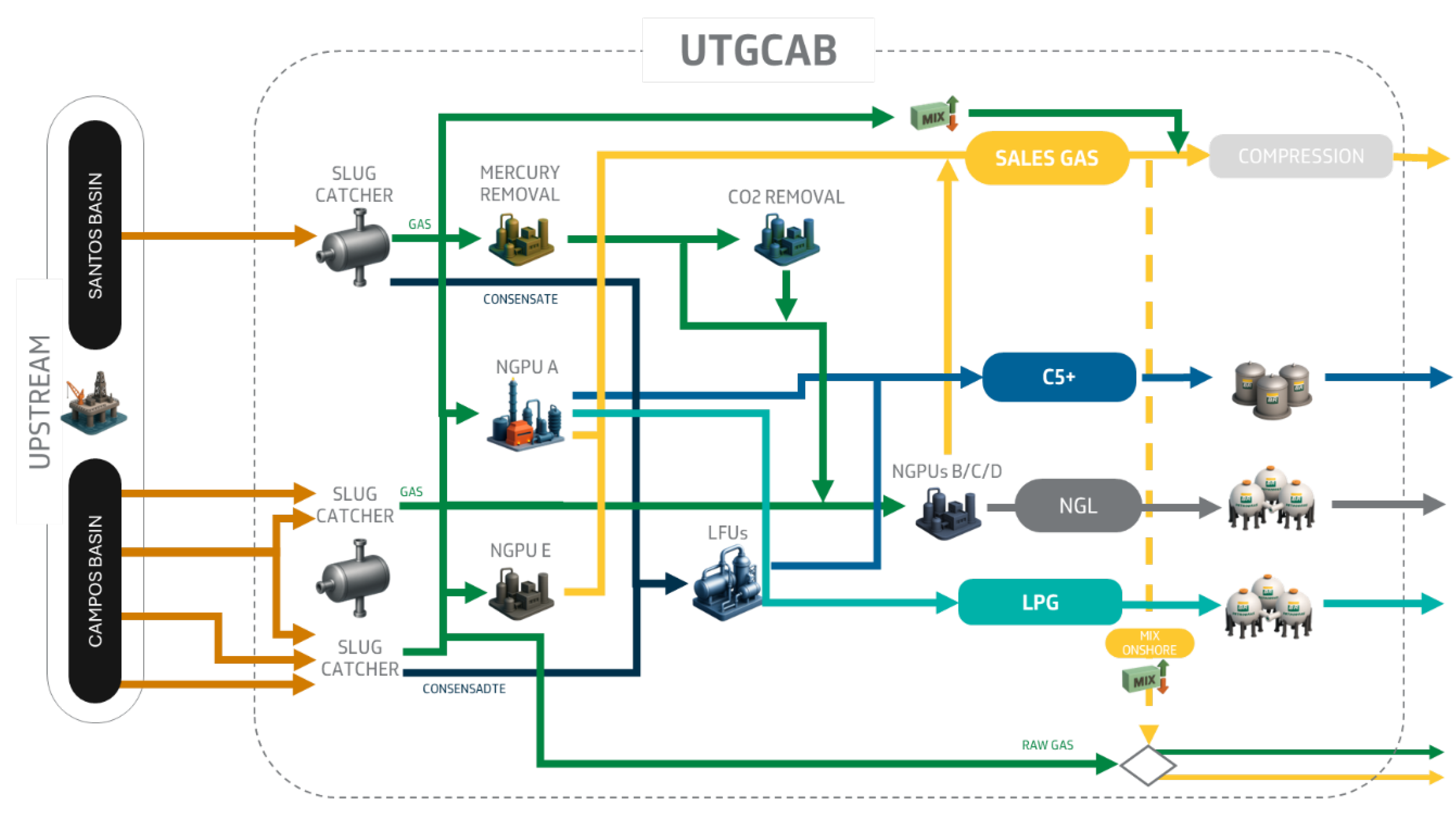
Figure 9.
Optimization history plot results of FNN architecture and hyperparameters.
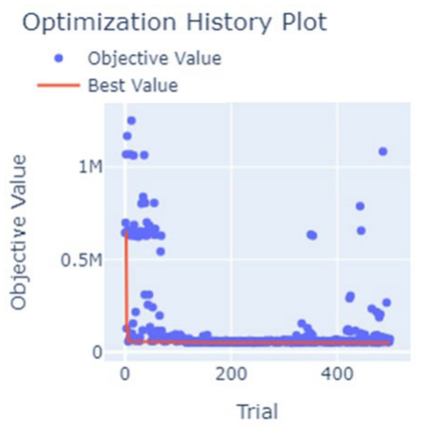
Figure 10.
Hyperparameter relative importance to the loss function, results of Optuna optimization.
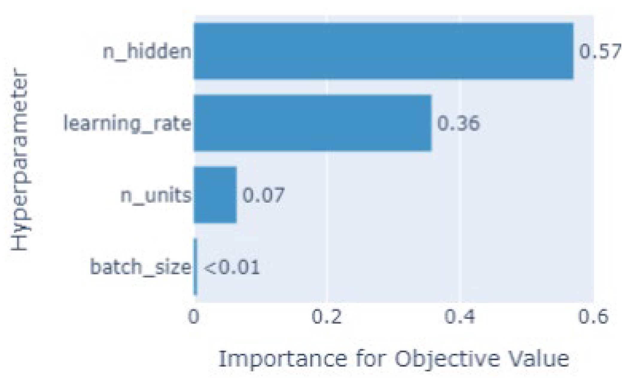
Figure 11.
Training and validation loss during FNN training. Horizontal axis represents the number of epochs.
Figure 11.
Training and validation loss during FNN training. Horizontal axis represents the number of epochs.
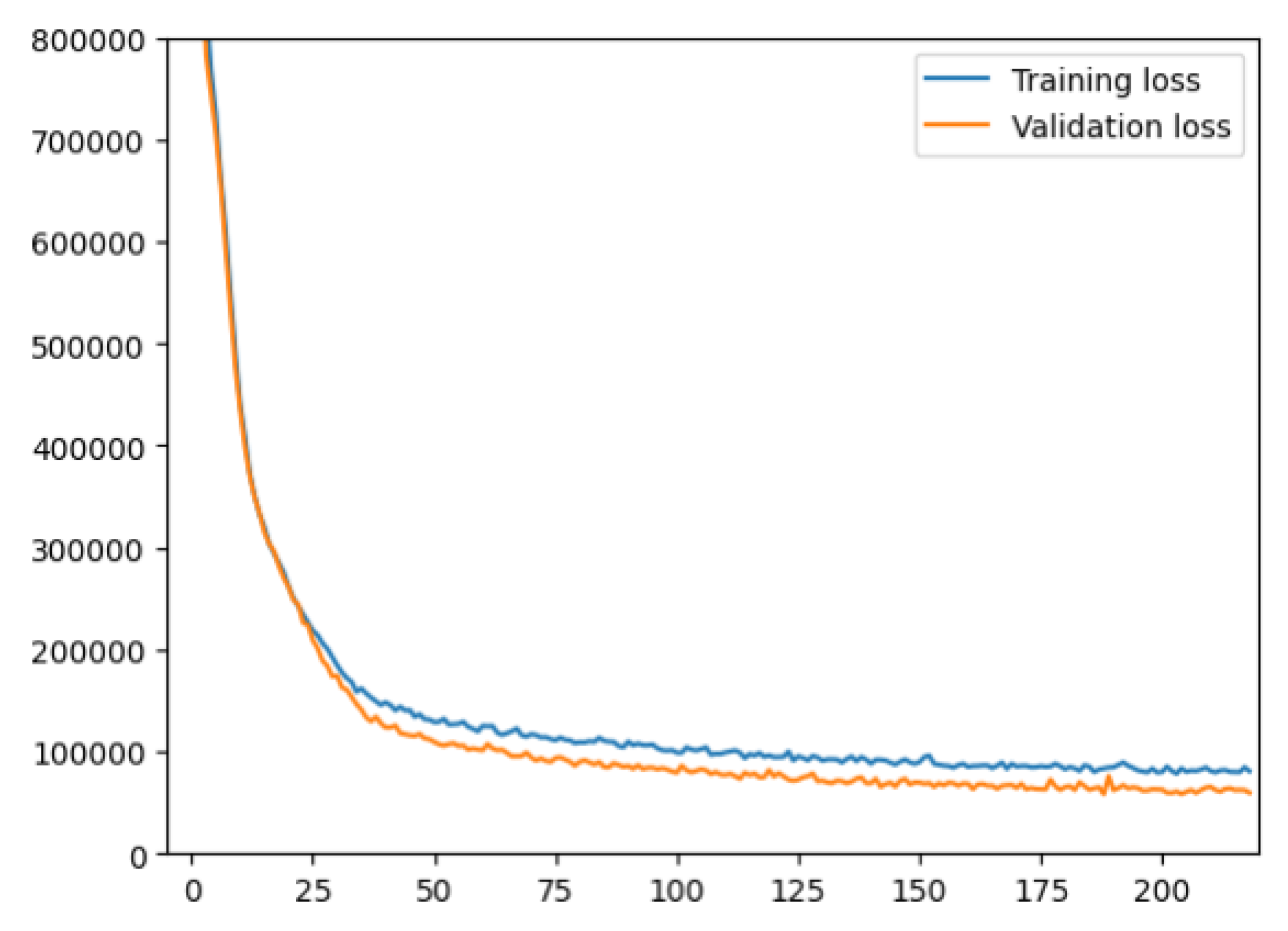
Figure 12.
Time-series plots of the 18 targets. Black lines are the actual y values and blue dashed lines are the values predicted by the FNN model.
Figure 12.
Time-series plots of the 18 targets. Black lines are the actual y values and blue dashed lines are the values predicted by the FNN model.
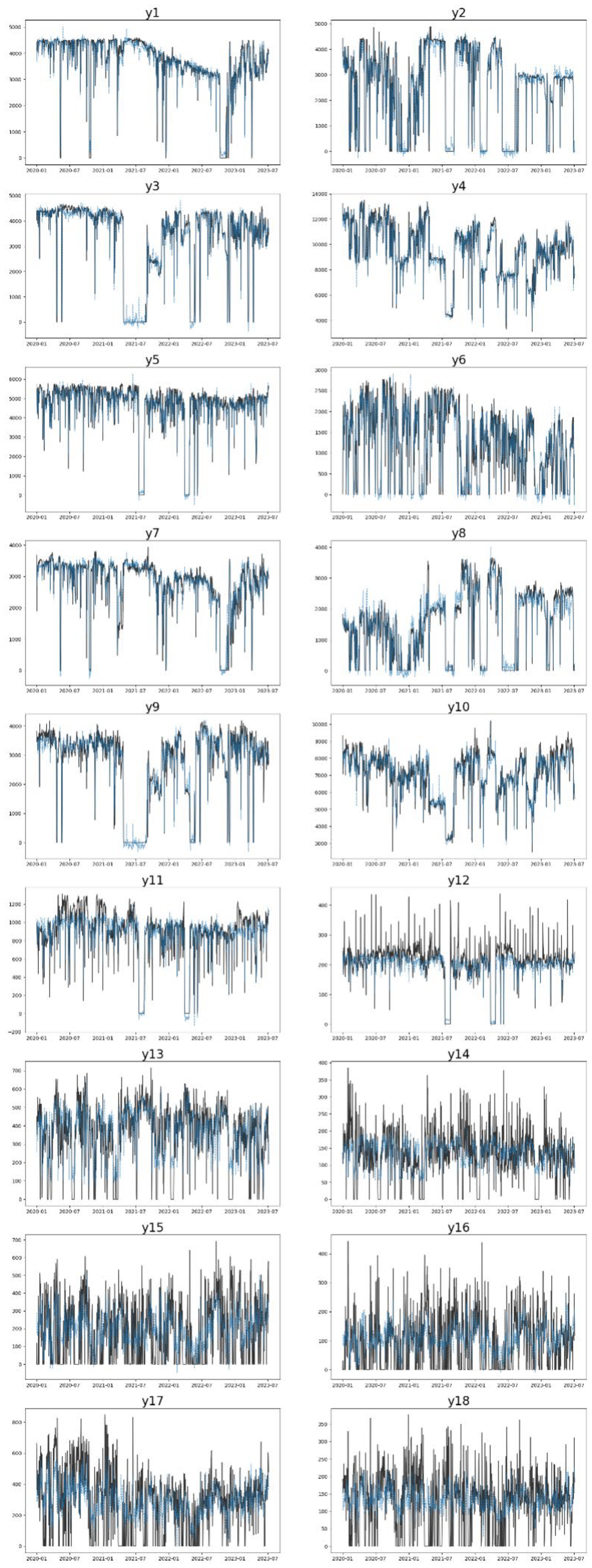

Table 1.
Search range of each manipulated parameter for architecture optimization of the neural network with Optuna.
Table 1.
Search range of each manipulated parameter for architecture optimization of the neural network with Optuna.
| Manipulated parameter | Search range |
|---|---|
| Number of hidden layers | 1 to 6 |
| Number of neurons per layer | 32 to 256 |
| Learning rate | 0.00001 to 0.1 |
| Batch size | [8,16,24,32] |
Table 2.
Best value of each manipulated parameter for architecture optimization of the neural network with Optuna.
Table 2.
Best value of each manipulated parameter for architecture optimization of the neural network with Optuna.
| Manipulated parameter | Best value |
|---|---|
| Number of hidden layers | 2 |
| Number of neurons per layer | 255 |
| Learning rate | 0.001533 |
| Batch size | 8 |
Table 3.
FNN final model architecture.
| Layer type | Output shape | Number of adjustable parameters |
|---|---|---|
| Dense | 225 | 5175 |
| Dense | 225 | 50850 |
| Dense | 18 | 4068 |
Disclaimer/Publisher’s Note: The statements, opinions and data contained in all publications are solely those of the individual author(s) and contributor(s) and not of MDPI and/or the editor(s). MDPI and/or the editor(s) disclaim responsibility for any injury to people or property resulting from any ideas, methods, instructions or products referred to in the content. |
© 2026 by the authors. Licensee MDPI, Basel, Switzerland. This article is an open access article distributed under the terms and conditions of the Creative Commons Attribution (CC BY) license (http://creativecommons.org/licenses/by/4.0/).
Copyright: This open access article is published under a Creative Commons CC BY 4.0 license, which permit the free download, distribution, and reuse, provided that the author and preprint are cited in any reuse.


