Submitted:
12 January 2026
Posted:
13 January 2026
You are already at the latest version
Abstract
Ice accretion along aircraft leading edges, particularly at stagnation line parting strips, remains difficult to remove using conventional electrothermal anti-icing systems. These systems require continuous high-power heating to maintain the stagnation region above the melting point, often exceeding 10–12 kW/m². This study introduces an Ice Cavitation Deicer (ICD) that removes ice through rapid, localized cavitation generated within a thin melt layer formed at the ice–surface interface. In the proposed approach, a short pulse of electric current melts a 1–10 µm interfacial layer and causes a cavitation impulse of approximately 1–10 MPa. This impulse ejects the stagnation line ice in a direction normal to the surface, often against the external airflow, enabling the immediate aerodynamic removal of the remaining ice. Analytical modeling based on the energy conservation principle was used to determine the optimal foil geometry, thermal pulse parameters, thermal stress, and material selection. Experiments with various metallic foils and substrate materials validated the predicted ejection behavior. Compared with conventional thermal anti-icing, the ICD concept reduces power consumption by approximately two orders of magnitude while offering rapid and reliable leading-edge deicing.
Keywords:
ice cavitation deicer (ICD)
; pulse electrothermal deicer (PETD)
; cavitation pressure
; stagnation-line deicing
; leading-edge deicing
; COMSOL Multiphysics
1. Introduction
Ice accretion on aircraft wings and engine inlets is a persistent hazard in aviation. When supercooled water droplets impact an airfoil, they may freeze on contact and form ice layers that alter the aerodynamic shape, reduce lift, increase drag, and in severe cases, lead to flow separation and loss of flight stability. The region of the wing leading edge that is most difficult to protect is the stagnation-line parting strip, where the local airflow velocity approaches zero and convective momentum transfer is minimal. Ice in this region adheres strongly to the surface and is resistant to both aerodynamic removal and mechanical shedding.
Conventional electrothermal anti-icing systems address this problem by supplying continuous high-power heating to the stagnation region to maintain it above the ice melting point. Typical power densities may reach 10–12 kW/m². The high power density imposes a substantial energy burden on aircraft electrical systems and limits their applicability to smaller platforms, such as unmanned aerial vehicles. Alternative pulse-based electrothermal deicers (PETDs [1,2]) reduce power by melting a thin interfacial layer between the ice and substrate; however, because the stagnation-line ice is not readily lifted by aerodynamic forces, PETDs alone are insufficient to remove ice from the critical region of the airfoil.
To overcome this challenge, we introduce an Ice Cavitation Deicer (ICD): a thin metallic or laminated foil that, when pulsed above the water cavitation temperature (≈ 300 °C), generates a rapid pressure impulse within the interfacial melt layer. This impulse can reach approximately 10–20 MPa [3,4], which is sufficiently high to fracture and eject ice in the direction normal to the surface, even against the external airflow.
The idea of leveraging high water vapor pressure to improve PETD performance was first proposed in 2010 by Petrenko [5], but it has never been investigated. When combined with an upstream PETD pulse that forms a thin melt layer (typically 0.01–0.1 mm thick), the ICD enables the rapid removal of stagnation-line ice that would otherwise remain attached.
In this study, the underlying theory of ICD operation was developed based on the energy conservation principle, thermal and mechanical constraints were evaluated, and COMSOL Multiphysics FEA simulations were used to optimize the foil geometry, heating rates, and material selection. Experimental demonstrations with metals and laminate foils confirmed the predicted cavitation-induced ice ejection. The results show that the ICD concept can reduce the stagnation line deicing power by approximately two orders of magnitude relative to conventional continuous electrothermal systems, offering a compact, energy-efficient, and fast-acting solution for aerospace deicing.
2. ICD Concept and Preliminary Criteria for the Selection of ICD Materials
Predicting cavitation is a formidable task, particularly in water [6]. Despite significant efforts and achievements, the study is still ongoing. However, no theoretical studies on ice cavitation have been performed to date. Because of the lack of information about ice cavitation, it is not productive to begin experimenting with a new phenomenon without an approximate set of calculations and numerical estimates of its effects on the system.
The following analytical and computer simulation analyses did not pretend to be accurate ICD theories; however, they have proven to be useful for selecting candidate materials and determining a range of appropriate experimental conditions.
First, we performed numerical calculations based on the energy conservation law (ECL). Although the ECL is an approximation, it is an effective tool. This study assumes that the electric energy initially stored in an ICD capacitor is used to heat a thin metal foil, heat-diffusion layers of the substrate and ice, and the resistive components of power electronics.
Figure 1 shows the ICD geometry used in this study. The metal foil is either attached to the substrate with a high-temperature adhesive or pressed onto the substrate by either a magnetic field (for ferromagnetic metals in laboratory experiments only) or by stretching it over a convex surface.
Combined PETD/ICD deicing system is shown.
2.1. Notations
Because the 36 variables are used in the theoretical part of the manuscript, for reader convenience, we collected the list and description of all the variables in one place below.
QICD is the density of the energy required for ICD (J/m2).
Qtot is the total density of the energy requirement of an ICD, which includes the circuit losses (J/m2).
TICD is the maximum (cavitation) temperature of the metal foil before cavitation occurs.
T0 is the initial temperature of air and that of the ICD, °C.
Tm is the ice-melting temperature, 0°C.
is the maximum temperature difference between two points in a material.
ρ is density, kg/m3.
C is the specific heat, J/(K∙kg).
qi is the latent heat of ice melting, which is 333 kJ/kg.
qw is the latent heat of water evaporation.
l is length, m.
w is width, m.
r is aspect ratio, l/w.
CC is the capacitance of an energy-storage capacitor, F.
V0 is the initial capacitor voltage, V.
tp is pulse length, s.
σ is the stress, Pa.
σTS is the thermal stress, Pa.
σyield is the yield stress, Pa.
α is the coefficient of thermal expansion (CTE), K−1.
µ is the shear modulus, Pa.
E is the elastic modulus, Pa.
γ is the CP/CV ratio of water vapor.
QC is the initial energy stored in the capacitor, J.
Rtot is the total serial resistance of the entire power circuit. This includes the resistance (ESR) of the capacitor, switch, metal foil, and lids, Ω.
ρe is electrical resistivity, Ω∙m.
Rm = ρe∙r/tm is the resistance of the metal foil, where tm is the material thickness, Ω.
Rrest = Rtot – Rm is the resistance of all other circuit components, lids, bus bars, ESR of the switch, and capacitor, Ω.
Ltot is the total inductance of the capacitor-discharge circuit, H.
g is the acceleration due to gravity, m/s2.
vice is the maximum ice velocity, m/s.
Tno_ice is the maximum ICD temperature in the absence of ice, °C.
ρv is the water vapor density at atmospheric pressure, Pa.
ρcav is water vapor density at cavitation pressure, Pa.
The subscripts s, m, i, and w denote the substrate, metal, ice, and water, respectively.
2.2. Calculations of the ICD Energy Requirement
The approximate ICD energy requirement can be determined by applying the energy conservation law as follows:
Equation (3) assumes that the energy delivered to the ICD is distributed through heat conduction across the metal foil, heat diffusion layers of the substrate, ice, and melted layer (i.e., water). The heat diffusion length in ice, is several times greater than that of water, . Equation (3) provides a simple approximation of the initial ICD design and optimization. More accurate results were obtained through COMSOL Multiphysics simulations, which are presented in the following sections of this paper.
Not all the energy stored in the capacitor is used to heat the metal foil and interfacial layers of the materials. A portion of the stored energy is lost in the components of an electric circuit. Therefore, the total ICD energy requirement, Qtot, exceeds QICD:
As shown in Figure 2, Qtot initially decreased with an increase in the aspect ratio of the foil, r, and then increased with a further increase in r. The initial decrease in Qtot was caused by an increase in the resistance of the foil and lower losses in the rest of the electric circuit. The subsequent increase in Qtot is due to the increase in the circuit time constant tp, which results in greater heat diffusion into ice and substrate.
The maximum temperature of the foils was TICD = 330°C, and the air temperature was T0 = −10°C. The heat diffusion length was calculated using equation (1), where tp = Rtot∙CC was the time constant of an over-damped RCL circuit. The sub “Proto” instead of “ICD” was used in our MathCad calculations.
The minimum ICD energy requirement shown in Figure 2 is common for all foil materials that were simulated and analyzed. The foil material properties are presented in Table A1 in the Appendix. The properties of the substrates are listed in Table A2.
In equation (1), tp represents the "thermal pulse length," which is the time required for approximately 90% of the total energy stored in the capacitor to be delivered to the ICD. Computer simulations show that when the circuit is over-damped, >>1, tp is approximately equal to . The minimum duration of RCL (Resistor-Capacitor-Inductor) circuit discharge occurred when =1. In this case:
is the fully damped circuit resistance, = 1:
is the electrical time constant of a fully damped circuit.
According to our computer simulation results (COMSOL Multiphysics; see below), the maximum ICD temperature of a fully damped RCL circuit was observed at the time:
For over-damped circuits, >> 1:
tp ≈ Rtot∙CC
In the following section, "Cavitation Pressure of Water and Its Work," it is shown that the total mechanical momentum exerted on the ice due to the vapor pressure increases with an increase in . Thus, circuits with a high dissipation factor (ζ >> 1) have been employed in applications where significant mechanical momentum is required for ice removal, despite the higher energy demand associated with such designs. The main contributor to the ICD energy requirement was the product of equation (3).
2.3. Overheating Ice-Free Areas of ICD
A critical parameter limiting ICD design is the maximum temperature Tno-ice, which is reached in the ice-free areas of the ICD. If the ICD is not properly designed, this temperature can easily exceed the maximum service temperature of the foil or substrate material. Using ECL, the following equation was derived for Tno_ice in the ICD’s ice-free areas:
Given TICD and Tno_ice, the ICD energy requirement in equation (3) was minimized for all materials used in this study. The results of this optimization are presented in Table 1. The minimum ICD total energy requirement, Qtot, was calculated for Tevap = 330°C, T.no_ice = 400°C, and CC = 1. 5,mF, and Rrest = 14mohm. The other properties of the materials are listed in Table A1 and Table A2 in the appendix.
2.4. Thermal Stress of ICD
Another design challenge for ICD is the high thermal stress of the metal foil and substrate material. When a material is constrained, the maximum thermal stress can be estimated as
For a material to withstand multiple ICD pulses, its yield or/and compression strength should be higher than the maximum thermal stress:
σyield > σTS
Appendix A and Appendix B present a comparison of σyield and σTS of the materials used in this study for . As can be seen, not all the materials tested or analyzed satisfied the requirements of equation (11). The most probable location of the maximum thermal stress in the metal foils was at the interfaces with the cold electrical busbars. This stress can be effectively reduced by heating the busbars using the same ICD electric pulse. The highest temperature gradients in the substrates occurred at the interface with hot metal foils.
Thermal Shear-Lag Problem for a Thin Foil Bonded by a Compliant Adhesive
This section addresses the classical thermo-mechanical shear-lag problem of a thin, stiff metallic foil bonded to a rigid substrate by a compliant adhesive layer and subjected to thermal loads. The problem is characterized by large in-plane aspect ratios and a strong stiffness contrast between the foil and adhesive, conditions under which full three-dimensional finite element modeling becomes computationally inefficient and numerically ill-conditioned.
The analytical framework employed in this study is rooted in the classical shear-lag theory originally introduced by Volkersen [7] for load transfer in bonded joints and subsequently developed in the context of adhesive joint mechanics by Goland and Reissner [8]. Subsequent aerospace-focused analyses by Hart-Smith [9] further established the applicability of shear-lag models to thin adherends bonded by compliant layers. Modern expositions of this theory can be found in standard texts on adhesively bonded joints.
In the present formulation, the adhesive layer is modeled as a distributed shear foundation that transmits only shear stress between the foil and rigid substrate. The effective shear stiffness per unit area of the adhesive layer is expressed as:
where ta is the adhesive thickness, and Geff is the effective shear modulus that accounts for possible through-thickness variations in adhesive properties.
When the shear modulus varies across the adhesive thickness, the effective modulus is defined by the harmonic mean of the local shear compliance as follows:
The axial equilibrium of the thin foil relates the gradient of the axial stress to the adhesive shear stress as follows:
where tf is the foil thickness.
The thermally induced axial stress in the foil was introduced using the following eigenstrain formulation:
where Ef and αf are the Young’s modulus and coefficient of thermal expansion of the foil, respectively, u is displacement and ΔTf is the temperature increase of the foil.
The shear-lag parameter β is defined as:
The inverse of β represents the characteristic stress transfer length that controls the degree of thermal constraint imposed by the adhesive layer.
For a uniformly heated foil of length L with traction-free ends, the closed-form solution of the governing equation yields a hyperbolic axial stress distribution. The maximum compressive axial stress occurs at the mid-length of the foil and is given by:
The corresponding adhesive shear stress distribution reaches its maximum magnitude at the foil ends. The maximum adhesive shear stress is expressed as:
These closed-form expressions provide a transparent and computationally efficient basis for estimating both foil axial stress and adhesive shear stress under extreme thermal loading, and are particularly well suited for adhesive selection and preliminary design of high-aspect-ratio laminated structures.
Figure 5 shows the maximum normal stress in the SS 17-7PH foil calculated using equation 17. The plateau in Figure 5 corresponds to the maximum thermal stress in the material. Flexible silicone-based adhesives have shear moduli below 10 MPa, and they can significantly reduce the maximum thermal stress in the metal foils of ICD. Ceramic- and silicate-based adhesives have shear moduli well over 100 MPa. Figure 6 shows the maximum shear stress in the SS 17-7PH foil calculated using equation 18.
The maximum shear stress in the adhesive layer was equal to the maximum stress in the foil. The maximum thermal stress in the adhesive layer is σTa =αa∙∆Tf∙Ea. The maximum total 2D stress in an adhesive layer is approximately equal to:
Figure 7 shows the dependence of the maximum and yield stress in the ICD made of Ti grade 5 and titanium grade 4 foils. The solid red line represents Ti grade 4 0.01 mm foil on 1 mm Cotronics 1531 silicone adhesive. The blue-dotted line is for Ti grade 5 0.01 mm foil on 1 mm silicate-based Cotronics 905 adhesive. The black-dashed line shows the yield strength of titanium grade 5 at 400°C. The dash-dot crimson line shows the yield strength of titanium grade 4 at 400°C.
The results of the foil stress calculations presented in Figure 7 confirm that grade 4 and grade 5 titanium foils on silicone adhesive can be safely used up to 1 m-long strips, and that grade 5 titanium foil can also be safely used on the silicate-based low thermal expansion Cotronics 905 adhesive (Cotronics 940LE is an option). The maximum and shear stresses using equations 17-19 have been conducted for foils made of molybdenum, Invar, Inconel 783, SS 17-7PH, tungsten, two high-temperature silicone adhesives, and several silicate and ceramic adhesives. The metal foils were attached to a solid base using silicone or silicate-based adhesives. The selective results of the calculations are presented in Table 3.
To avoid the thermal stress caused by the mismatch of the CTE in several laboratory ICDs, no adhesion was used, and the metal foils were pressed to the substrate either by magnetic pressure for ferromagnetic materials or by stretching the foil over a cylindrical cylinder, as described in Section 3. The adjacent moving layers of the ICDs glide over each other with friction. The friction force was calculated by multiplying the friction coefficient by the normal pressure. The maximum cavitation pressure should be added to thermal stress.
2.5. Cavitation Pressure of Water and Its Work on Ice Sheet
The experimental data on the cavitation pressure of water in the temperature range of 300–370°C can be approximated using the following fitting formula:
where Pcav in equation (12) is the fitting function of the experimental data [4,6]. Although the available cavitation threshold temperature data are scattered, their average is approximately (300±10) °C. Hence, 300°C was used in Equation (20).
The cavitation pressure of water can reach 20MPa at 370°C. This pressure was developed in a thin interfacial layer of melted ice. The formation of this high-pressure vapor layer (or bubbles) can induce further evaporation of the melted layer, and the resulting pressure expels the ice sheet from the ICD. The maximum work conducted on ice by the expanding cavitated layer was approximated under the assumption of purely adiabatic vapor layer expansion, which ceased when the vapor pressure decreased to atmospheric pressure. The equations 21-25 present the results of the maximum work calculations:
where tcav is the thickness of the interfacial water layer heated over 300°C:
Note that this layer is very thin: =0.33 mm,=1.04 mm:
is the adiabatic work done by the water vapor:
is the expected maximum velocity of the ice layer. This assumes that all the work is performed on ice.
Figure 8 shows the dependence of the initial thickness of the cavitating layer on the maximum temperature of the foil.
Figure 9 shows the estimated maximum velocity of a 5-mm thick ice sheet at the maximum temperature of the metal foil TICD.
Table 2 lists the parameters of the ICD made of a 17-7PH foil attached to a solid substrate with a 1 mm thick silicone adhesive. The parameters were used to build an actual ICD prototype and to calculate the ICD electrical current and foil temperature, as shown in Figure 10 and Figure 11.
Figure 11 shows the time dependence of the current, and Figure 11 shows the time dependence of the maximum SS foil temperature. Figure 11 indicates that the interfacial temperature reached 330°C at 400 µs after most of the initial electric charge (approximately 90%) passed through the foil, as shown in Figure 10.

Table 3.
Examples of COMSOL and MathCad results for selected ICDs.
| Materials | Dimensions | QICD | vice | σmax | τmax | Tno_ice |
|---|---|---|---|---|---|---|
| Foil/substrate | mm | kJ/m2 | m/s | Mpa | MPa | °C |
| W/CA_905 1.0mF x 1100V |
0.027 x 40 x 340 | 45 | 1.5 | 540 | 0.526 | 400 |
| W/SA 1.0mF x 1100V |
0.033 x 28 x 320 | 53.6 | 2 | 264 | 0.5 | 400 |
| SS 17-7/SA_1531 2 x 1.5mF x 1100V |
0.0254 x 78 x 466 | 50 | 1.7 | 47 | 0.165 | 415 |
| SS 17-7/CA_905 2 x 1.5mF x 1100V |
0.025 x 85 x (2 x 428) | 50 | 3.5 | 1000 | 6.6 | 450 |
| Invar/Loctite 1.5mF x 1100V |
0.015 x 184 x 106 | 45.4 | 6.6 | 185 | 0.84 | 400 |
| Ti Gr4/SA_1531 2 x 0.5mF x 1100V |
0.028 x 33 x (2 x 261) | 35.5 | 1.5 | 44 | 0.01 | 400 |
| Ti Gr4/SA_1531 1.5mF x 1100V |
0.05 x 36 x 394 | 64 | 9.2 | 27 | 0.014 | 406 |
| Ti Gr5/CA_905 2 x 0.5mF x 1100V |
0.03 x 76 x (2 x 114) | 35.5 | 1.5 | 413 | 3.8 | 400 |
| Mo/SA 1.5 mF x 1000V |
0.0254 x 47 x 450 | 35.4 | 5.6 | 21 | 0.137 | 400 |
Table 3 presents the most important calculation results for the selected ICDs. In all these examples, the environmental temperature was T0 = −10°C, and the ICD maximum temperature was TICD = 330 °C. Silicone adhesives were either Permatex Optimum silicone adhesive substrate with Tmax = 399 °C, or Cotronics Duraseal 1531 with Tmax = 427 °C. solid substrate. The maximum von Mises thermal stresses in the metal foils and substrates were given at the maximum temperatures of no-ice areas.
2.6. Summary of Materials Analysis
- Invar, tungsten, titanium grade 5, and SS 17-7PH have shear strengths higher than their maximum thermal stress at 400 °C. The foils made of these metals can be used with any HT adhesive analyzed in this study.
- Any metal foil analyzed in this study can be safely attached to a solid base using the two analyzed HT silicone adhesives.
- The main cause of thermal stress in the adhesive is the temperature gradient at the interface with the hot metal foil. Only two HT silicone adhesives, two Cotronics low-expansion silicate-based adhesives, and the composite-material silicate-based LOCTITE 2000 adhesive have strengths higher than their maximum thermal stress at 400 °C.
- Oxidation in air above 400 °C limits the use of tungsten, Invar, and titanium grade 5.
- The overall winners among the metals were SS 17-7PH and Ti grade 4 on Cotronics 1531.
- The overall winners among the adhesives were Cotronics 1531 silicone adhesive and Cotronics 905 and 940LE low-thermal-expansion silicate-based adhesives.
3. Experimental Work
All experiments were conducted at the Ice Research Lab of Petrenko-Multiphysics LLC. Various metals and metal alloys were investigated through the theoretical calculations to identify the optimal foil and substrate materials for experimental testing. Eleven metals were selected for this experiment. The properties of all materials used in this study are listed in Table A1 and Table A2. Below, we provide the rationale for selecting materials for the laboratory testing.
3.1. Metals Selection
Titanium Grade 4 (99% Ti) is the most commonly used grade in the aerospace industry. It has a low Cm∙ρm product, a CTE of approximately one half that of 304 and 316 SS, high corrosion resistance up to 426 °C, high strength, and high electrical resistivity.
Titanium Grade 3 was selected because of its low Cm∙ρm product, low CTE, and high corrosion resistance. It is suitable for ICD testing when attached to a silicone adhesive.
The Invar (Ni 36%, Fe 64) alloy was selected because of its exceptionally low CTE, high strength, mild corrosion resistance, ferromagnetic properties, and high electrical resistivity.
Stainless steels 304 and 316 are economical materials available in a wide range of thicknesses (starting from 0.005 mm and above). Under the “full-hard” condition, they offer high strength, corrosion resistance, and high electrical resistivity. However, their CTE values were higher than those of the SS 17-7PH and Inconel 783 alloys.
A 9-µm copper foil on a 25-µm Kapton film laminate was chosen because of its very low energy requirement as an ICD device material. This commercially available DuPont product can endure short heating pulses of up to 400°C.
17-7PH stainless steel was selected for its ferromagnetic properties, exceptional strength, high electrical resistivity, lower CTE than SS 304/316, and high corrosion resistance.
430 stainless steel was selected for its ferromagnetic properties, high strength, high electrical resistivity, and high corrosion resistance.
Nb was selected because it has the lowest Cm∙ρm product and a low CTE, which matches that of the Resbond 907 ceramic adhesive used in this study. Nb exhibits high corrosion resistance and mechanical strength (cold-rolled foils).
Tungsten has a very low Cm∙ρm product, a very low CTE, high mechanical strength, and good corrosion resistance.
Low-carbon 1008 steel has excellent magnetic properties and is easy and convenient to use in experiments. It is not corrosion-resistant and has a very modest strength.
Inconel 783 has an exceptional combination of high strength, low CTE, and corrosion resistance.
3.2. Substrate Materials Selection
Adhesives that can withstand temperatures over 400°C are primarily based on inorganic components, such as ceramics (CA), glass, or silicates (Si). These materials, while exceptionally heat-resistant (with only slow heating rates), form rigid and brittle bonds with metals rather than elastic ones. They are also more likely to fail under thermal shock or stress because of their significant CTE and low flexibility. After evaluating a large number of commercially available CA and SI adhesives, we found only three such adhesives that can be used as ICD substrates. The first was the LOCTITE MR 2000 composite adhesive manufactured by Henkel Co. According to the adhesive datasheet, its compressive modulus is 295MPa or almost two orders of magnitude lower than that of ceramic adhesives. As shown in Table A2, the thermal stress in LOCTATE MR 2000 can be lower than its compressive strength. The second and third adhesives were Cotronics 905 and 940LE silicate-based adhesives.
More opportunities arise from the use of two high-temperature silicone adhesives. The first is the Permatex Optimum silicone adhesive substrate with Tmax = 399 °C, and the second is the Cotronics 1531 silicone adhesive with Tmax = 427 °C.
3.3. Measurements of Ice Velocity
We used two methods to measure the maximum initial velocity of the ice fragment. In the first method, we played back video clips of ICD deicing frame by frame with 1/60 s between frames. During the ICD tests, the ice fragments were propelled rapidly away from the deicing surface. In many demonstrations, the fragments reached velocities on the order of 10 m/s. At typical smartphone frame rates (10–60 fps), the fragments move between 0.17 and 1 m per frame, leaving the field of view in 1–2 frames. This provides an insufficient temporal resolution for accurate frame-based tracking. Therefore, video footage is primarily used for the qualitative confirmation of ICD performance.
In the second method, the initial horizontal velocity was obtained using a simple ballistic equation. The ICD was positioned 1.0 m above the carpeted floor, and the horizontal travel distance of the detached ice fragments was measured. Assuming a negligible initial vertical velocity, the flight time is determined by free fall:
where and
The initial horizontal velocity is then expressed as
This method significantly improves the velocity precision compared to frame counting. For the demonstrated ICD configurations, the measured velocities were typically , depending on the laminate design and the pulse parameters. These experimental results agree well with the theoretical estimates based on vapor expansion impulse generation.
For quick and simple tests of the ferromagnetic foils, they were attached to solid substrates with magnetic shields, as shown in Figure 12. The maximum magnetization of such shields was B=1.2T, which pressed the foils to the substrate by up to PM= B2/2µ0 =574kPa. While keeping the foils in place, the magnetic support allowed the foils to expand and contract without significant thermal stress. The shear stress was limited by the friction coefficient of the material used. Although this attachment method worked very well in our laboratory tests, we do not recommend it for real applications because of the possible wear of the contacting materials.
3.4. Electronics
Figure 13 shows the electric circuit used in this study. The MOC223 optocoupler isolates the low-voltage trigger circuit (left) from the high-voltage ICD circuit (right). The two diodes protect the capacitor and semiconductor-controlled rectifier (SCR) from reverse-voltage peaks. The peak capacitor discharge currents during testing varied from 200A to 12 kA. The SCR consisted of four parallel BT158W thyristors, each capable of withstanding a 3 kA 1-ms current pulse with an I²t rating of 6,000 A²s. Because of the low resistance of the tested ICDs, most connections were soldered, and 12 and 14 AWG leads were used to minimize the total resistance in high-current circuits. The capacitor charger module delivered an output power of 60 W with a maximum output voltage of 900 V. All the capacitors used in this study were film capacitors, featuring a very low estimated series resistance (ESR) of approximately 1 mΩ. The circuit shown in Figure 12 was used for several hundred pulses during the test period.
3.5. Experimental Results
The results of the selected tests are presented in Table 4. The air temperature for all tests was set to −10°C. The successful performance of the ICDs was video recorded and is available in the Supplementary Media Files of this manuscript.
Table 4 presents the experimental conditions and maximum ice-fragment velocities. *0.1 mm mica film on a magnet paper sheet (Figure 11). M < 0.1T. ** ICD foil was stretched over a Porcelain ceramic cylinder with tight contact but with no adhesive. *** 0.1mm Mica film on a conformable magnet sheet for irregular surfaces, M = 0.42T, as shown in Figure 15.
**** 0.1mm Mica film on an array of small 2mm x 5mm x 20mm Neodymium magnets N52, M = 1.2T. M is the magnetization provided by the supplier. CA is a mica-based ceramic adhesive #907 from Cotronics Inc. SA is a Permatex Optimum Red 399C silicone adhesive.
The maximum normal pressure of the magnet was M2/(2µ0). However, owing to the small thickness of the ferromagnetic foil, the actual pressure was lower than the calculated value. We calculated the actual normal pressure using COMSOL Multiphysics software.
All ICDs, which were constructed from the selected materials and designed according to the theoretically calculated parameters, successfully demonstrated the ice cavitation phenomenon. The best deicing performance was observed with 0.0762 mm thick 17-7PH stainless steel and titanium Grade 4 0.05 mm thick foil, which exhibited the highest ice expulsion velocity of 6–10 m/s.
The lowest energy consumption for the ICDs was achieved using the thinnest foil. However, the thinnest SS foil lacked durability and exhibited signs of strain after several ICD pulses were applied. The Cu/Kapton laminate produced by DuPont did not exhibit signs of strain after 25 ICD-pulse tests. Neither did 10 µm Ti foil, which was stretched over a ceramic cylinder. The lower the product of the material density and specific heat capacity, the lower the energy requirement for the ICD.
The best ICD performance was achieved when a metal foil was attached to a rigid substrate, such as a cylindrical solid ceramic surface (** porcelain), Cotronics 907 ceramic adhesive (CA), and an array of small neodymium magnets (N52) (****).
Figure 13 shows the dependence of the ice fragment velocity on the estimated maximum temperature of the SS foil. The thermal time constant of the stainless-steel ICD was 0.15 ms. Data were collected from the test results of ICDs made of stainless steel 17-7PH. The maximum foil temperature was calculated using the ECL equation. The ice velocity increased with increasing maximum foil temperature and tp, which agrees with the theory.
Ice cavitation effectively separated the ice from all the metal foils. The theoretical predictions and experimental results showed reasonable agreement, suggesting that the developed theory could be beneficial for future practical applications of ice cavitation.
While the trend line in Figure 13 points at a Tcav of 310 ±10°C, it may be lower on highly hydrophobic surfaces. Thomas et al [10] observed that Tcav depends on the hydrophobicity or hydrophilicity of the surface. For highly hydrophobic coatings (e.g., CH3(CH2)15SH), cavitation occurred at temperatures as low as 187–197°C. They also noted a reduction in Tcav with an increase in the heating pulse duration. This observation is not surprising because prolonged heating eventually causes water to boil at 100°C. Most experimental data on Tcav originate from studies using gold and platinum wires as heaters, with electric pulse lengths ranging from 1 to 5 µs. In contrast, our experiments used much longer heating pulses, ranging from 30 µs to 1 ms.
The reduction of Tcav (our TICD) can be used to further reduce the ICD energy requirement, as shown in Equation (3) and Figure 4.
The ice fragment velocities presented in Figure 13 agree with the theoretically calculated velocities presented in Figure 8.
Niobium and titanium foils demonstrated a low ICD energy requirement and good de-icing performance, making them strong contenders for material selection. Moreover, the CTE of Nb closely matched that of the 907-ceramic adhesive.
The lowest experimentally observed ICD energy requirement, 11.25 kJ/m², was found for the very thin (0.01 mm) titanium ICD. However, titanium is the most challenging material to work with, because soldering titanium instantly creates a thick and poorly conductive oxide layer. We successfully attached nickel bus bars to titanium foils using an ultrasonic solder and a solder alloy, Cerasolzer 217, developed specifically for soldering titanium. Unfortunately, the initially low resistance of the nickel busbars (1mΩ) increased significantly after several ICD pulses, following the degradation of the ICD performance. Durable low-resistance electrical connections to titanium require titanium electroplating with Ni. However, only a limited number of companies worldwide claim to have the capability to electroplate titanium with nickel, and their services are prohibitively expensive for laboratory-scale testing. Nevertheless, the excellent performance of ICDs made of titanium Grades 3 and 4 (vice ≥ 6 m/s) and the modest energy requirement (≤ 77 kJ/m2) make titanium attractive for this application.
Invar-made ICDs demonstrated reproducible results, although their performance was not particularly impressive. For ICD applications, Invar offers high electrical resistivity (8.2 × 10⁻⁷ Ω·m), sufficient yield strength (260 MPa at 400 °C), modest corrosion resistance, and ferromagnetism. Invars can also be easily soldered. The magnetic properties of Invar foils allow them to be attached to substrates without adhesives, thereby avoiding high thermal stress. However, the ferromagnetism of Invar diminishes above temperature of 279°C. The very low temperature-average CTE of Invar (2.5 × 10⁻⁶ K⁻¹) results in a relatively low thermal stress, even when a ceramic adhesive is used. Owing to the high strength of Invar, thin Invar foils should also withstand rain-erosion tests. ICDs made of 0.008 mm (commercially available Invar foil thickness) have a very low energy requirement of 28 kJ/m², making Invar a strong candidate for ICD applications. These thin Invar foils must be bonded to a solid substrate using Cotronics 905 or Cotronics 940LE adhesives. Invar exhibits limited corrosion resistance at temperatures below 450°C.
The ICD made of very thin 304 stainless steel demonstrated a very low energy requirement. However, 304 stainless steel has a relatively large CTE and insufficient strength (Table A1). However, this steel cannot be used in large-scale applications.
The ICD made of 430C stainless steel demonstrated an acceptable ICD performance. However, 430C stainless steel has insufficient strength (Table A1). However, this steel cannot be used in large-scale applications.
We observed the best overall performance for ICDs made of martensitic 17-7PH stainless steel. This steel has exceptional strength, a modest CTE, and high corrosion resistance. The ICD made of this steel can be attached to substrates using two silicone adhesives and two silicate-based low-thermal-expansion adhesives.
The copper/Kapton laminate (Pyralux AC by Dupont Co.) exhibited the third lowest energy density requirement of 25.5 kJ/m2. However, copper has a very low yield strength and cannot be used for large-scale applications.
3.6. Absence of Cavitation Damage (CD)
We have been experimenting with ICDs since 2005 (the time when we worked on the patent application), testing over 50 combinations of metals and substrates at various temperatures, power rates and energy densities. The overall number of tests was over 1000. However, no signs of cavitation damage were observed. (Hundreds of cavitation damage images are available on the web for comparison). We provide a video clip of ICDs in action. The video shows the 35th test of a 17-7PH cold rolled 3 mil thick foil placed on Cotronics 907 CA. The second clip shows the 25th test of a 9 µm copper/25µm Kapton laminate stretched over a ceramic cylinder, D = 10 cm. We did not observe any water-cavitation damage to the ICDs. We believe that the absence of CD is due to the confinement of the µm-thick cavitating liquid film between the two solids, as shown in Figure 1. The maximum steam pressure of the thin water film cavitation (1–10 MPa) was much lower than the strength of ICD foils. Moreover, we did not find any published images of CD formed at temperatures of 300 °C or higher. CD occurred at temperatures below the water boiling point when the negative cavitation pressure was very large (170MPa to 200MPa). This high pressure is one to two orders of magnitude higher than the maximum pressure of an ICD.
4. Feasibility of a Full-Scale ICD
The ICD dimensions used in our laboratory tests were selected to fit the dimensions of our refrigerators and the specifications of our high-voltage electronics. However, can ICDs deice large aircrafts? To answer this question, we performed the following calculations using the dimensions of the ice-protected areas of the Boing 787-9 aircraft [10].
Aice = 20.95 m2 is the total ice-protection area of the Boeing 787. The area was divided into eight slats for cyclic deicing.
Aps = Aice∙0.19 = 3.98 m2 is the total parting strip area that was continuously heated, and tdeicing = 3 min is the recommended period for cyclic deicing [11].
For the ICD operations, we selected three 3.0 mF x 1100V thin-film capacitors (EPCOS-TDK). Each capacitor was assigned one-third of the Aps. (assuming two wings and a stabilizer area). A 0.025 mm thick SS 17-7PH foil with Cotronics 905 silicate-based low-thermal-expansion adhesive was selected as the ICD material.
CC = 3 mF.
VC = 1100 V is the initial voltage of the capacitor.
The ICD design is presented in the 3th and 5th rows of Table 3. The 3.0 mF capacitor powers the two connected ICD sections in parallel, as listed in Table 3. 1.5mF per section.
Qtot = 50 kJ/m2 is the total ICD energy density requirement ( Table 3).
WICD = Qtot/tdeicing = 278 W/m2 is the time-averaged ICD power requirement.
Assuming a 90% efficiency of the capacitor chargers, the time-averaged ICD power requirement is:
WICD_total = WICD/0.9 = 309 W/m2
Please compare the above number with the 18.60 kW/m2 of the SAE recommendation for the continuous heating of the parting strips.
The energy stored in the capacitor is QC = CC ∙ VC2/2 = 1.815 kJ.
AICD = QC/Qtot = 0.036 m2 is the area of ICD section.
NICD = Aps/AICD = 111 is the total number of ICD sections, that is, 37 sections per capacitor.
The total time required to deice the parting strips is limited by the charging time of one capacitor multiplied by the number of ICD sections per capacitor.
Pcharge is the capacitor charger output power, and
tcharge = QC/(Pcharge × 0.9) is the time required to charge the capacitor, assuming 90% efficiency.
tICD = tcharge∙ NICD/3 is the total time required to deice all parting strips.
With 9 kW (3 kW per charger) delegated to the ICD system, the total time was 25 s, which is a small fraction of the de-icing cycle (180s). For comparison, the Boeing 787 has two generators with a total power output of 500 kW. The A320 Airbus Airplane has an electric power of 180 kW. Increasing the total deicing time of the ICD to 3 min reduced the average total ICD power requirement to 1.2 kW.
Note that the 3 mF film capacitor has an Equivalent Serial Resistor) of 1mohm, which is approximately 1% of the ICD ESR. Thus, only a few watts will be dissipated inside the capacitor. The capacitor has a weight of approximately 2 kg and does not overheat.
In the above estimates, we neglected the ICD pulse length, which is less than 1ms.
The high voltage of 1100V can be reduced by using aluminum electrolytic capacitors of similar size and weight as the 3.0 mF x 1100V film capacitor. For instance, a 39 mF x
500VDC HCG FA capacitor manufactured by Hitachi can store 4875 J of electrical energy. This is almost three times more than the energy stored in a 3 mF x1100V capacitor.
The 18 mF x400V capacitor by Nippon Chemi-Con closely matched the energy stored in the 3.0 mFx1100V capacitor. As a reference, the onboard voltage of 240VAC is commonly used in aviation, and it has a 340V amplitude.
The maximum ICD temperatures of 350–450 °C were well below the aircraft engine exhaust temperature of 788–955 °C.
Combining an ICD for parting strips with a synchronized PETD for the remaining iced areas of the airfoils can significantly reduce the energy and power consumption required for aircraft deicing.
The integration of the ICD into an entire aircraft deicing system is the focus of our ongoing research. However, owing to the very low power and energy requirements, the ICD can perform deicing of the total icing area instead of being complementary to the PETD or cyclic deicing.
5. Conclusions
This study introduces and experimentally validates the Ice Cavitation Deicer (ICD), a new deicing technology capable of removing ice from the leading edge of airfoils with extremely low energy consumption. The ICD uses short, intense thermal pulses to superheat a thin interfacial melt layer and generate a cavitation impulse in the range of 1–10 MPa. The impulses were sufficient to fracture and eject the ice in the direction normal to the surface. Cavitation impulses accelerate ice fragments to 5–10 m/s, ensuring rapid detachment. Theoretical calculations accurately predicted foil heating, melt-layer thickness, cavitation pressure, thermal stress of ICD materials, and uplift velocity, validating the theoretical framework.The ICD operation reduces the average deicing power by approximately two orders of magnitude compared to the continuous electrothermal heating of the stagnation line.The selected metal foils and adhesives withstood repeated thermal cycling, demonstrating their suitability for long-term aerospace operations.
Overall, the Ice Cavitation Deicer provides a compact, energy-efficient, and highly effective method for removing stagnation line ice. Its low power requirements, rapid response, and compatibility with thin-foil heater architectures make it a promising technology for both conventional and electrified aircraft, UAVs, rotorcraft, and other platforms where power availability is limited. Future work will focus on scaling the ICD to full leading-edge geometries, optimizing the laminate structures, and integrating the system into flight-capable prototypes.
Supplementary Materials
Clip 1. Stainless-steel foil on a ceramic adhesive. A stainless steel 17-7PH foil was attached to a ceramic plate using ceramic adhesive (907 by Cotronics Inc.). The foil dimensions were 0.076 mm × 20 mm × 150 mm. CC = 1.5 mF, V0 = 760V, Qtot = 144 kJ/m2, Tair = -10 °C. Ice cubes measuring 10 mm × 10 mm × 10 mm were attached to the foil with rapidly freezing water drops. The initial velocity of the ice fragments exceeded 10 m/s.
Funding
This research was funded by Petrenko-Multiphysics, LLC.
Data Availability Statement
Data supporting the findings of this study are available from the author upon reasonable request.
Acknowledgments
The author gratefully acknowledges the funding and laboratory facilities provided for this research by Petrenko-Multiphysics LLC.
Conflicts of Interest
The authors declare no conflicts of interest. The author is an inventor of patents related to the deicing technologies described in this study.
Appendix
Table A1.
Properties of metals at 400°C-450°C.
| Material | ρ | C | α | ρe | k | E | σyield at 400°C | σts at 400°C |
| Units | kg/m3 | J/kg∙K | K-5 | 10-8 W∙m | W/m∙K | GPa | MPa | MPa |
| Invar, as rolled, Tmax ≤ 400°C |
8100 | 515 | 0.3 | 82 | 10.2 | 125 | 240-280 | 140 |
| SS 17-7PH, CH900 Tmax = 482 °C |
7800 | 460 | 1.1 | 83 | 16.4 | 204 | 1200 | 780 |
| Ti Grade 5, TH1050 Tmax ≤ 400°C |
4430 | 526 | 0.85 | 178 | 7 | 114 | 800 | 400 |
| Ti Grade 4 as rolled Tmax = 426 °C |
4540 | 523 | 0.85 | 56 | 17 | 116 | 150 | 360 |
| Tungsten cold rolled Tmax ≤ 400°C |
19300 | 134 | 0.4 | 5.4 | 163 | 300 | 600-700 | 625 |
| Molybdenum TZM Tmax = 400°C |
10220 | 217 | 0.5 | 5.3 | 130 | 330 | 650-780 | 700 |
| Inconel 783 Tmax = 700 °C |
7810 | 435 | 11 | 120 | 11.4 | 173 | 750 | 727 |
| SS 304 Tmax ≤ 400°C |
||||||||
| SS 304 full hard | 7900 | 450 | 1.7 | 72 | 17.3 | 200 | 140 | 1384 |
| SS 430C | 7740 | 460 | 1.1 | 60 | 26 | 200 | 190 | 864 |
| Nb cold rolled Tmax ≤ 400°C |
8570 | 268 | 0.7 | 16 | 53 | 103 | 300 | 288 |
The mechanical properties of metal and metal alloy foils are strongly dependent on the details of their manufacturing, such as being as-rolled, annealed, or cold rolled.
SS 17-7PH CH900 temper is a cold-rolled material heat-treated at 900 °F (482°C) for one hour after forming.
Table A2.
Properties of substrate materials.
| Substrates | ρ | C | α | Tmax | k | E | σyield at 400°C | σts at 400°C |
| Units | kg/m3 | J/kg∙K | K-5 | °C | W/m∙K | GPa | MPa | Mpa |
| SA, Cotronics | 998 | 1465 | 2 | 427 | 0.3 | 0.0012 | 1.9 | 0.01 |
| SA, Permatex | 1180 | 1050 | 30 | 399 | 0.2 | 0.0014 | ≈5.5 | 0.14 |
| Kapton | 1420 | 1090 | 1.7 | 400 | 0.12 | 2.5 | 234 | 17 |
| Cotronics 905 | 1310 | 800 | 0.054 | 1370 | 1.44 | ≈7.5 | 22 | 0.0016 |
| Cotronics 940LE | 1310 | 800 | 0.072 | 1370 | 0.72 | ≈7.5 | 24 | 0.0021 |
| Zr ceramic flex ribbon | 6000 | 540 | 1.08 | 1000 | 2.7 | 210 | 1000 | 860 |
| Upilex | 1400 | 1100 | 2.0 | ≤450 | 0.13 | 7.5 | 530 | 52 |
| Loctite 2000 | 1540 | NA | 0.7 | 1000 | 1.2 | 0.3 | 2.4 | 0.83 |
| Anodized Ti | ≤ 4000 | 683 | ≈0.85 | ≥700 | ≈ 2.3 | ≈ 40 | ≈ 3500 | 140 |
Comments on the above-listed materials: Yellow shading indicates fully acceptable materials for use in ICD. SA Permatex is a Permatex Optimum Red 399C silicone adhesive. SA Cotronics was Duraseal 1531. The green shading marks the materials with marginal performance in ICD applications. No-color shading marks the materials that are unacceptable either because of insufficient strength or low service temperature.
References
- Petrenko, V.F. Systems and methods for modifying an ice-to-object interface. US Patent 6,870,139, 2005.
- Petrenko, V.F.; Sullivan, S.R; V. Kozlyuk, V.; Petrenko, F.V.; Veerasamy, V. Cold Reg. Sci. Technol. 2011, 65(1), 70-78.
- Caupin, F; Herbert, E. Cavitation in water: A review. C. R. Phys. 2006, 7, 1000-1017. [CrossRef]
- Caupin, F. Liquid-vapor interface, cavitation, and the phase diagram of water. Phys. Rev. 2005, E 71, 051605-1-051605-5. [CrossRef]
- V. F. Petrenko, V.F. US Patent 7,703,300. 2010.
- Magaletti, F.; Gallo, M.; Casciola, C.M. Water cavitation from ambient to high temperatures. Nature Portfolio, Scientific Reports. 2021, 11, 1-10.
- Volkersen, O. Die Nietkraftverteilung in zugbeanspruchten Nietverbindungen mit konstanten Laschenquerschnitten. Luftfahrtforschung 1938, 15, 41–47.
- Goland, M.; Reissner, E. The stresses in cemented joints. J. Appl. Mech. 1944, 11, A17–A27.
- Hart-Smith, L.J. Adhesive-Bonded Single-Lap Joints; NASA CR-112236, 1973.
- Thomas, O.C.; R. E. Cavicchi, R.E.; M. J. Tarlov, M.J. Effect of Surface Wettability on Fast Transient Microboiling Behavior. Langmuir. 2003, 19, 6168-6177. [CrossRef]
- Meier, O.; Scholz, D. Handbook method for estimating power requirements for electrical de-icing systems. Hamburg University of Applied Sciences, Hamburg, Germany. 2010. https://www.fzt.hawhamburg.de/pers/Scholz/MOZART/MOZART_PRE_DLRK_10-08-31.pdf.
Figure 1.
Figure 1. ICD geometry prior to expansion of the cavitation layer (yellow) of the melted ice.
Figure 1.
Figure 1. ICD geometry prior to expansion of the cavitation layer (yellow) of the melted ice.
Figure 2.
Total ICD energy requirement, QICD (J/m2) vs aspect ratio of a foil r, calculated with equations (3) and (4) for the 0.03 mm Invar foil (solid red line) and for the Tungsten 0.025 mm foil (blue dotted line). The base material was porcelain ceramic.
Figure 2.
Total ICD energy requirement, QICD (J/m2) vs aspect ratio of a foil r, calculated with equations (3) and (4) for the 0.03 mm Invar foil (solid red line) and for the Tungsten 0.025 mm foil (blue dotted line). The base material was porcelain ceramic.
Figure 3.
The optimized total energy density requirement, J/m2 (red solid line), and the optimized tungsten ICD foil thickness, m (blue dotted line) vs. temperature of the ice-free areas. Tevap = 330°C, CC = 1.5 mF, and Rrest = 14mohm. The sub “Prot_W” instead of “tot” was used in our MathCad calculations.
Figure 4.
Total energy density requirement, J/m2 (red solid line), and tungsten ICD foil thickness, m (blue dotted line) vs. maximum ICD temperature, Tevap. Tno_ice = 400°C, CC = 1.5 mF, and Rrest = 14mohm. The sub “Prot_W” instead of “tot” was used in our MathCad calculations.
Figure 4.
Total energy density requirement, J/m2 (red solid line), and tungsten ICD foil thickness, m (blue dotted line) vs. maximum ICD temperature, Tevap. Tno_ice = 400°C, CC = 1.5 mF, and Rrest = 14mohm. The sub “Prot_W” instead of “tot” was used in our MathCad calculations.
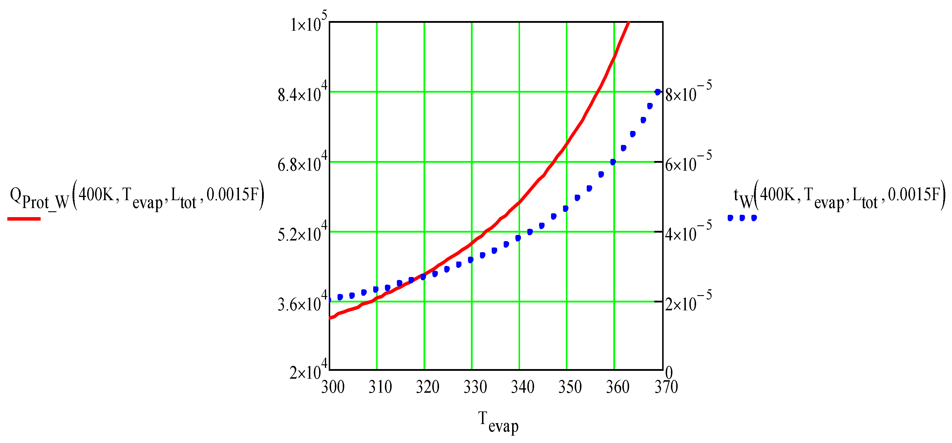
Figure 5.
Dependence of the maximum stress in the ICD foil made of SS 17-7PH, σ17_7, Pa, on, shear modulus of adhesive, µa, Pa. The length of the foil was 50 cm, and its thickness was 0.076 mm. Equation 17 was used. The SS 17-7PH yield and maximum strength at 450C shown for reference.
Figure 5.
Dependence of the maximum stress in the ICD foil made of SS 17-7PH, σ17_7, Pa, on, shear modulus of adhesive, µa, Pa. The length of the foil was 50 cm, and its thickness was 0.076 mm. Equation 17 was used. The SS 17-7PH yield and maximum strength at 450C shown for reference.
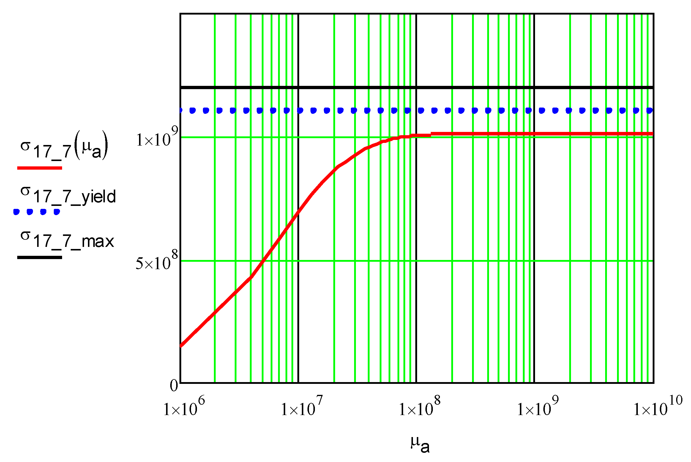
Figure 6.
Dependence of the maximum shear stress in the ICD foil, SS 17-7PH (Pa), on the shear modulus of the adhesive, µa (Pa). The foil length was 50 cm, and the thickness was 0.076 mm. Equation 18 was used.
Figure 6.
Dependence of the maximum shear stress in the ICD foil, SS 17-7PH (Pa), on the shear modulus of the adhesive, µa (Pa). The foil length was 50 cm, and the thickness was 0.076 mm. Equation 18 was used.
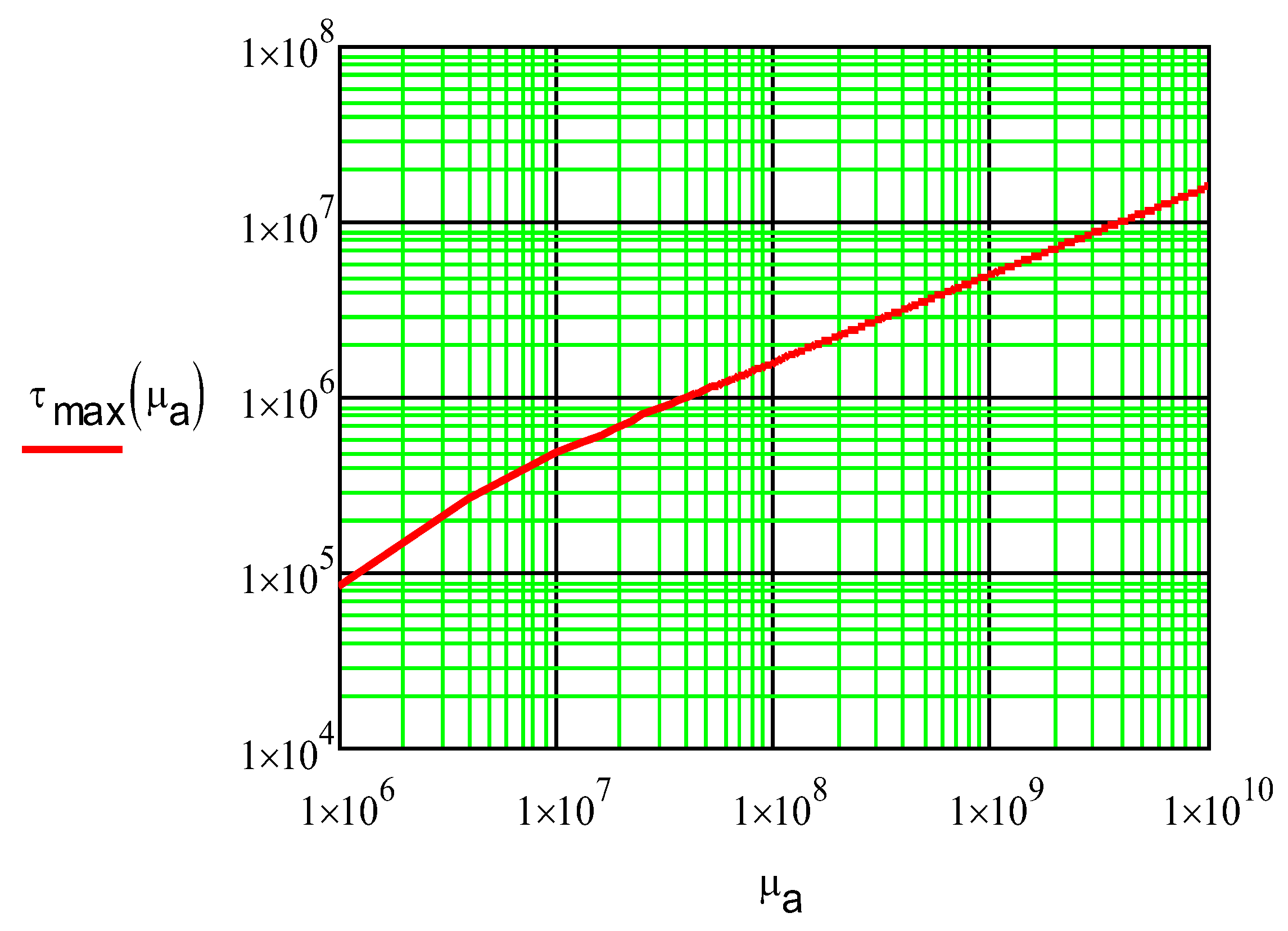
Figure 7.
Dependence of the maximum and yield stress in the ICD made of Ti grade 5 and titanium grade 4 foils, σmax (Pa), on foil length, m, at T.max = 400°C.
Figure 7.
Dependence of the maximum and yield stress in the ICD made of Ti grade 5 and titanium grade 4 foils, σmax (Pa), on foil length, m, at T.max = 400°C.
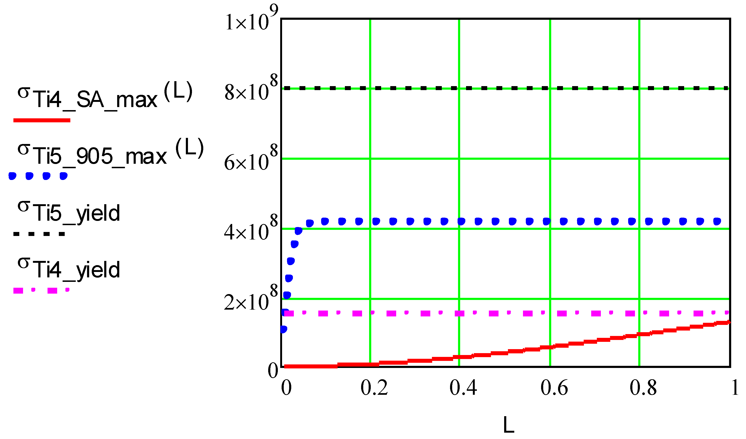
Figure 8.
Thickness of cavitating layer, m, vs. cavitation temperature, °C. tp= 1ms.
Figure 9.
Ice velocity (m/s) vs. cavitation temperature (°C) The thickness of the ice layer was 5 mm. red solid line), (blue-dot line).
Figure 9.
Ice velocity (m/s) vs. cavitation temperature (°C) The thickness of the ice layer was 5 mm. red solid line), (blue-dot line).
Figure 10.
Electrical current, A, vs. time, s, COMSOL simulation of 17-7PH stainless-steel ICD on mica laminate.
Figure 10.
Electrical current, A, vs. time, s, COMSOL simulation of 17-7PH stainless-steel ICD on mica laminate.
Figure 11.
Maximum temperature of 17-7PHSS foil, degree C, vs. time, s, COMSOL simulation of 17-7PH stainless steel/SA laminate ICD.
Figure 11.
Maximum temperature of 17-7PHSS foil, degree C, vs. time, s, COMSOL simulation of 17-7PH stainless steel/SA laminate ICD.

Figure 12.
Magnetic attachment of ferromagnetic foils.
Figure 13.
Schematic diagram of the electronics used to test the ICD prototypes.
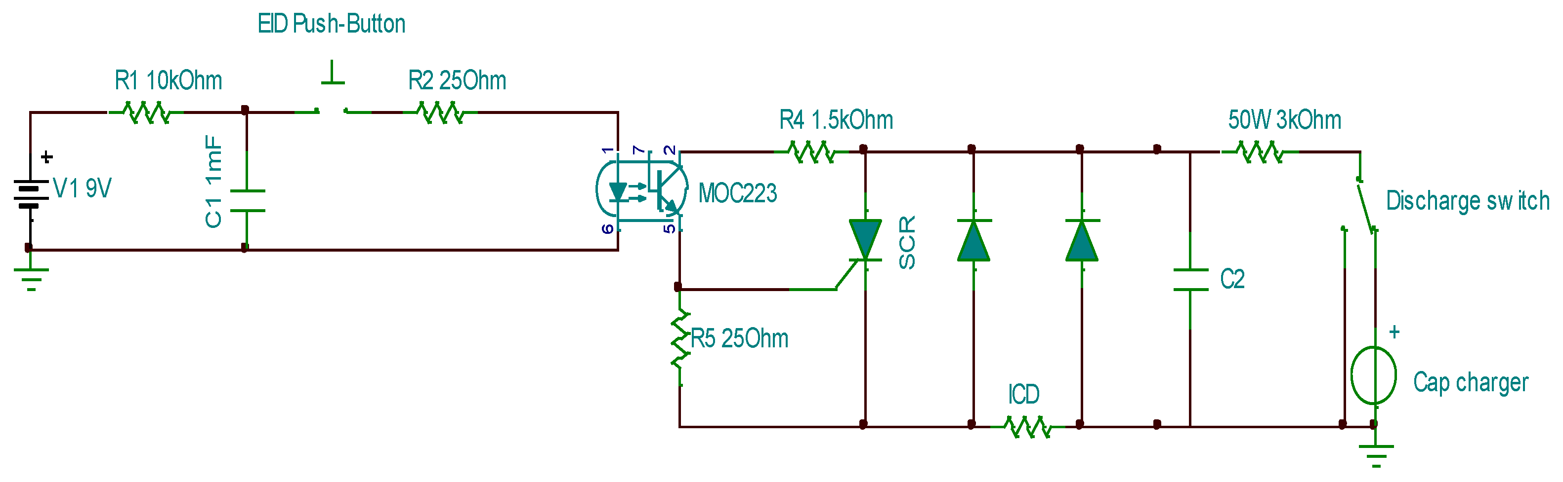
Figure 13.
Approximate velocity of ice fragments, m/s, versus maximum SS foil temperature, °C.
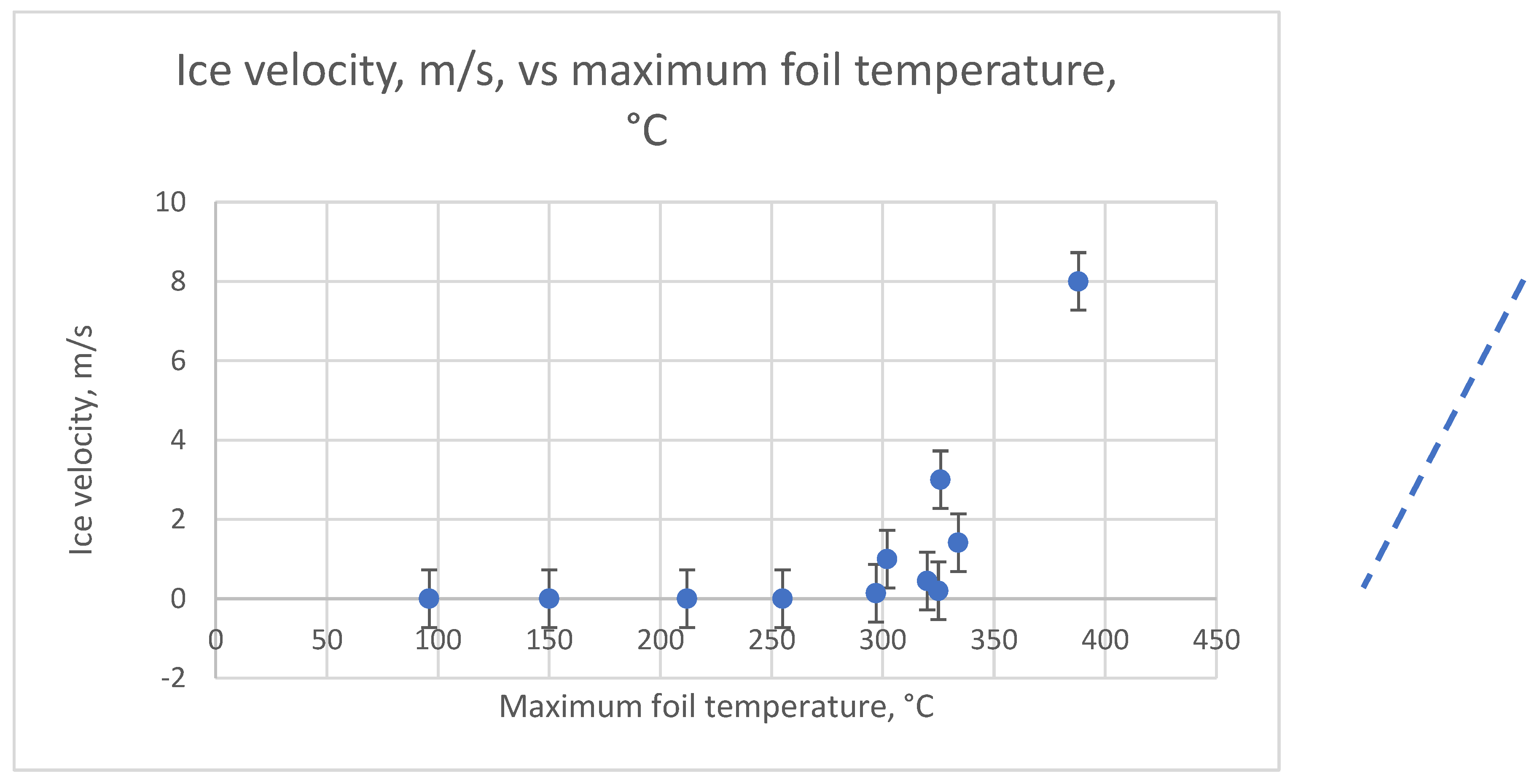
Table 1.
The minimum ICD total energy requirement.
| Material | r=l/w | Thickness mm | τp, ms | Qtot, kJ/m2 |
|---|---|---|---|---|
| 17-7PH SS | 0.789 | 0.0194 | 0.061 | 42.9 |
| Nb | 4.8 | 0.035 | 0.072 | 48.25 |
| W | 11.6 | 0.031 | 0.072 | 49.1 |
| Ti | 1.466 | 0.034 | 0.072 | 49.3 |
| Invar | 0.69 | 0.019 | 0.071 | 49.1 |
| SS440C | 1.13 | 0.023 | 0.072 | 49.4 |
| SS304 | 0.922 | 0.023 | 0.072 | 49.3 |
Table 2.
Parameters used to model ICD made of 17-7PH SS.
| T0 | -10[degC] | 263.15 K | Ice initial temperature |
| t_SA | 1[mm] | 1 mm | Silicone adhesive thickness |
| t_SS | 3[mil] | 7.62E-5 m | Foil thickness |
| t_ice | 100[um] | 1E-4 m | Ice thickness |
| dT | 5[K] | 5 K | Phase transition width |
| V0 | 720[V] | 720 V | Initial capacitor voltage |
| C | 1.5[mF] | 0.0015 F | Capacitor capacitance |
| l | 15[cm] | 0.15 m | SS foil length |
| w | 2[cm] | 0.02 m | SS foil width |
| R0 | ro_e*l/(w*t_SS) | 0.128 Ω | Foil resistance |
| Rc | 0.0011[ohm] | 0.0011 Ω | Capacitor ESR |
| Rsw | 0.0009[ohm] | 9E-4 Ω | SCR (switch) ESR |
| Rw | (0.0077+0.003)[ohm] | 0.0107 Ω | Lids and bus bars resistance |
| Lc | 8.4e-7[H] | 8.4E-7 H | Total circuit inductance |
| Xi1 | Rtot1*sqrt(C/Lc)/2 | 3 | damping factor |
| Q | C*V0^2/(2*l*w) | 130 kJ/m2 | ICD energy density, J/m2 |
| Rtot | ro_e*l/(w*t_SS)+Rc+Rw+Rsw | 0.142 Ω | Total circuit resistance |
| Qevap | Q*R0/Rtot | 108 kJ/m2 | ICD foil energy requirement |
Table 4.
Summary of selected experimental results. Not all the test results are shown.
| Foil | Substrate | Size, mm | V0, V | CC, mF | Qtot,kJ/m2 | vice,m/s |
| Invar | *Mica | 0.03 × 31.2 × 107 | 550 | 1.5 | 68 | ≈1 |
| Ti Grade 4 | ** Porcelain | 0.05 × 20 × 158 | 570 | 1.5 | 77 | ≥ 6 |
| Ti Grade 3 | ** Porcelain | 0.01 x 37 x75 | 790 | 0.1 | 11.25 | ≥2 |
| SS 17-7PH | *** Mica | 0.0762 × 20 × 140 | 760 | 1.5 | 155 | ≥8 |
| SS 17-7PH | **** | 0.0762 × 15 × 150 | 600 | 1.5 | 120 | ≥6 |
| SS 17-7PH | CA | 0.0762 × 20 × 140 | 700 | 1.5 | 130 | 6.6 |
| SS 17-7PH | ** Porcelain | 0.0762 × 20 × 150 | 750 | 1.5 | 140 | ≥10 |
| SS 17-7PH | SA | 0.0762 × 20 × 150 | 720 | 1.5 | 130 | ≥4 |
| SS 430 | *** Mica | 0.054 × 18 × 91 | 460 | 1.5 | 97 | ≈2 |
| SS 304 | 3M HT tape | 0.0127 × 25.4 ×38 | 314 | 0.383 | 19.6 | ≈1 |
| Cu/ Kapton | ** Porcelain | 0.009 × 14 × 214 | 400 | 0.735 | 25.5 | ≥2 |
| Niobium | CA | 0.03 × 12 × 118 | 320 | 1.5 | 54 | ≥1 |
Disclaimer/Publisher’s Note: The statements, opinions and data contained in all publications are solely those of the individual author(s) and contributor(s) and not of MDPI and/or the editor(s). MDPI and/or the editor(s) disclaim responsibility for any injury to people or property resulting from any ideas, methods, instructions or products referred to in the content. |
© 2026 by the authors. Licensee MDPI, Basel, Switzerland. This article is an open access article distributed under the terms and conditions of the Creative Commons Attribution (CC BY) license (http://creativecommons.org/licenses/by/4.0/).
Copyright: This open access article is published under a Creative Commons CC BY 4.0 license, which permit the free download, distribution, and reuse, provided that the author and preprint are cited in any reuse.


