
Submitted:
12 January 2026
Posted:
13 January 2026
You are already at the latest version
Abstract
This study presents a prospective attributional Life Cycle Assessment of the Italian na-tional electricity grid for 2024–2040, aligned with the integrated national climate and en-ergy plan and the country's decarbonization pathway. The main goal was to calculate, analyze, and apply hourly emission factors for electricity and compare them with annual average factors for the same consumption profile to assess temporal effects on environmental outcomes. Hourly factors were derived from a cost-optimization energy model simulating Italy's evolving generation mix. The model projects a sharp decline in fossil-based generation and a significant expansion of solar photovoltaics and wind, which together exceed half of national production by 2040. Natural gas remains essential for system balancing, while electricity imports stabilize the grid when renewable output is low. 16 impact categories were evaluated, revealing decreasing trends in climate change (255 to 141 g CO2-eq/kWhe), acidification, and others, and rising temporal variability in mineral/ metal resource depletion and land use due to renewable intermittency. Applying the method to a positive energy district in Bologna shows that time-resolved factors offer clearer insights than annual averages, especially for season-dependent impacts, and demonstrate substantial reductions in impact by 2040, alongside notable differences between consuming and exporting electricity.
Keywords:
dynamic life cycle assessment
; prospective life cycle assessment
; electricity mix modeling
; hourly profiles
; energy systems
; environmental impacts
; positive-energy districts
1. Introduction
We live in a world of constant (climate) change. As humans, we play a significant role in shaping this increasingly complex reality, in which ecosystems and climate patterns are more unbalanced than ever. Undoubtedly, anthropogenic perturbation of these cycles must be studied in full detail, so that impacts are reduced, adaptation and mitigation strategies are enhanced, and, ideally, humanity can delay as much as possible the occurrence of the "tipping points" predicted by the scientific community [1]. These comprise three categories (melting, biome shift, and circulation change) of potential irreversible changes to Earth that can directly compromise humankind's existence and have certainly prompted countries to act before it is too late.
After all, climate change is not just about the Earth rising. Still, it is also reflected in water acidification, changes in precipitation patterns, sea level rise, eutrophication of soils, loss of biodiversity, glacier melting, poor air quality, and proliferation of infectious diseases, among many other physical impacts that affect humans daily. Since the Kyoto Protocol in 2005, major countries around the globe have begun announcing and enforcing environmental policies primarily targeting reductions in greenhouse gas emissions [2]. Under this scope, there is an inherent need to control and quantify the application of these strategies, and it is here that applicable international standards become extremely relevant.
Since the early 1970s, Life Cycle Assessment (LCA) has emerged as a key methodological framework for quantifying and standardizing the environmental impacts associated with human activities [3]. LCA evaluates the environmental burdens of a product or service across its entire life cycle, encompassing resource extraction, transportation, manufacturing, use, and end-of-life disposal. By providing a comprehensive and systematic perspective, LCA enables the identification of environmental hotspots and trade-offs within complex supply chains. However, this holistic approach often entails significant methodological challenges, particularly when life cycle stages are controlled by multiple actors and involve geographically dispersed processes [4]. The methodological principles and requirements of LCA are formalized in the ISO 14040 and ISO 14044 standards [5,6].
From an energy-sector perspective, electricity represents the most critical product for environmental assessment, as it is expected to form the backbone of the ongoing energy transition. Compared to alternative energy vectors such as hydrogen or biodiesel, electricity offers superior performance in terms of economic viability, energy efficiency, and land-use intensity. Its high transmission efficiency—often exceeding 90%—and relatively low infrastructure footprint have made electricity the most practical and scalable option for decarbonizing energy systems. Moreover, the electrification of heating, cooling, and urban transport is increasingly widespread, driven by improved conversion efficiencies and reduced carbon intensities relative to conventional fossil-based technologies [7].
Despite its central role, quantifying the environmental impacts of electricity generation is inherently complex and must not be oversimplified. The rapid integration of intermittent renewable energy sources into national grids has introduced substantial temporal variability in environmental impacts. Seasonal resource availability, fluctuating demand profiles, electricity imports, and operational constraints in balancing supply and demand all contribute to significant intra-annual variations. These dynamics are particularly relevant when assessing regional environmental burdens and designing effective decarbonization strategies.
As Bastos et al. [10] accurately note, most LCA studies of electricity generation over the past few years present annual generic averages to quantify its impacts. This practice ignores seasonal fluctuations in the availability of renewable resources, demand patterns, the availability of imported electricity, technical constraints on matching supply and demand, etc. Yet, all this needs to be considered to achieve a complete and convenient interpretation of the electrical system and to allow policymakers to understand consumption and generation patterns better, while at the same time advancing burden-sharing and environmental trade-off strategies, resource allocation, and impact-reduction optimization in the benefit of society. Furthermore, the LCA, especially in the energy sector, is often linked to greenhouse gas emissions in measuring national decarbonization strategies.
In this work, an attributional, prospective, average LCA framework is adopted. In this case, the assessment determines the environmental impact for which the product is responsible (impact allocation), rather than expanding the product system to identify all the consequences of consuming the product (consequential approach) [8]. Likewise, as Arvidsson et al. [9] describe, a prospective approach considers the development and evolution of a given technology over time, which makes room for environmental guidance as its impacts are quantified. There is an implicit choice of technology alternatives and modelling of foreground and background systems. Finally, this assessment is limited to average results on impacts and does not include a marginal demand analysis, which could be interesting as a part of future work.
1.1. Previous Work on the Topic
From an Italian standpoint, there has been significant research in this field, demonstrating a deep interest in measuring the country's decarbonization goals and the effects of its public policies. After all, despite the Italian current electricity mix still being 46% made up of natural-gas-fed sources, 4% of coal plants (accounting for a dramatic participation decrease in the past years), and 1% by oil generation technologies, renewables have been penetrating the electricity matrix at a fast pace [10].
Furthermore, 2030 has been identified as the year by which the main energy efficiency, grid decarbonization, and renewable capacity objectives are to be achieved, not only in Italy but in almost every country around the world. It is important to remember that the European Union (EU), through the European Climate Law (EU 2021/1119), set out the regional objective of reaching net-zero emissions by 2050, and the intermediate goal of reducing greenhouse gas emissions by 55% in 2030 with respect to 1990 levels. The official government document outlining the goals to be achieved in Italy by the mentioned year is the Integrated National Energy and Climate Plan (Piano Nazionale Integrato Energia e Clima - PNIEC) [11], which aligns with the European energy objectives established in the 2023 "Fit-for-55" and "RepowerEU" plans.
The PNIEC, directed to the European Commission, became public on the 30th of June 2024 and was written by the Italian Ministry of Environment and Energy Security (MASE) and the Italian Ministry of Infrastructure and Transport (MIT), in collaboration with other ministries like the Ministry of Economy and Finance (MEF). It targets objectives related to reducing polluting and climate-altering emissions, improving national energy security, and creating economic and employment opportunities for households and productive systems. Likewise, it mentions a strong interest in ensuring compatibility between energy and climate goals and environmental, air, and water quality, biodiversity, soil, and "green-heritage" objectives. With respect to the 2019-PNIEC scenario, objectives were re-evaluated and remeasured due to past implementation challenges, regulatory hurdles, and the recent, abrupt economic slowdown.
As an example of existing previous work, Garigulo et al. [12] assessed the annual based (static) environmental impacts of electricity in Italy in the single year 2030 following the "2019-PNIEC-proposed scenario and its comparison with respect to the EU reference scenario." It used 2017 as the base year and considered different impact categories, including: climate change, ozone depletion, particulate matter, ionising radiation, photochemical ozone formation, acidification, terrestrial eutrophication, freshwater eutrophication, marine eutrophication, and mineral, fossil, and renewable resource depletion. This last category was highlighted as one to target and consider in burden trade-offs, given the high levels of metals in the inverters and aluminum frames of PV modules. Yet, the absence of intra-year variations of the retrieved environmental factors of work represents its biggest limitation.
Similarly, Carvalho et al. [13] evaluated and compared the 2018 and 2030-PNIEC-envisioned Italian electricity mixes with those of other European Union member states, namely Belgium, Denmark, Finland, France, Germany, Portugal, and Spain. "EUref 2030" energy mix scenarios were considered for this. Again, impact assessment covers a broad spectrum of environmental consequences but still falls short in the time-variation aspect. The Italian national electricity plan was considered ambitious for foreseeing a 50% reduction in climate change impacts. In this work, the Eurostat platform [14] was used before ecoinvent [15] for some fuels and generation typologies that were absent in the latter LCI database. An increase in resource consumption was (again) linked to a reduction in CO2 eq emissions.
Moreover, Bastos et. al. [16] provide the closest and most updated contribution from this work's standpoint, in which an hourly predictive LCA model was developed. Two scenarios (PNIEC-2030 and Advanced-2030) were simulated with the EnergyPLAN tool, coupled with a Multi-Objective Evolutionary Algorithm, to optimize capacity expansion [17]. As for the hourly dispatch, which by far represents the most challenging part of the model, it was optimized using the Oemof framework [18]. This project confronted present-day (2018, 2019, and 2020) with alternative 2030 scenarios and attributed the main variations in environmental impacts to the increased penetration of renewables envisioned by the Italian energy goals. The analysis went even further by considering marginal electricity demand covered by unconstrained technologies.
Complementing this revision, Peters et al. [17] conducted an interesting analysis of the expected evolution of the Brazilian electric sector over the time horizon 2025-2050 across three transport sector transition scenarios. Time resolution was five years. Electric grid composition evolution was made by the Open-Source Energy Modeling System (OSeMOSYS). An annual LCA evaluating 10 impact categories was presented, as well as a "weighted multi-objective optimization" used to manage electricity generation sources to minimize climate change burden and the levelized cost of electricity.
Additionally, Messagie, M. et al. [18] highlighted the need to know the hourly CO2-eq emission factors within the context of (smart) electricity-consuming appliances, such as electric vehicles and heat pumps. The analysis was restricted to the LCA characterization of the Global Warming Potential (GWP) of 1 kWh of electricity in Belgium in 2011, from raw material extraction to actual electricity production. Demand patterns and the availability of electricity-generating sources were identified as the main drivers of hourly fluctuations in the environmental burden of electricity, offering an opportunity to optimize ecological performance in smart grids.
Evidently, prior research has been expanding gradually over the years. This responds to local and global calls for climate action through measurable, quantifiable policies. Common features in the literature include the widespread use of ecoinvent (version 3) [16] as the main LCI database, which, among others, uses the method "Allocation, cut-off by classification", which allocates burdens among co-products depending on whether they are goods or wastes. Recycled materials are said to start at zero burden (cut-off), while waste producers do not carry treatment burdens.
By bringing together country-specific data, this platform tries to provide appropriate supply chains for whole regions. The authors claim that extrapolation from single regions to larger or other geographies is performed when data are absent, which can lead to higher uncertainty. However, as the database is increasingly fed with regional data, extrapolated global background datasets are expected to become less relevant. In fact, in the literature review by Vetroni-Barros et al. [19], SimaPro, which directly integrates the ecoinvent dataset, was used in 12 of the 38 revised case studies. Other well-known platforms are GaBi, GEMIS, Umberto, and ECO-it. This review also highlights the need to develop region-specific LCIs across countries to improve robustness in the field.
Revision of national and local reports on historical electricity generation is also widespread among the studied publications. In Italy, the country's largest Transmission System Operator (TSO) for the grid, TERNA, reports annually all data related to the electricity supply and consumption chains. This is considered the most trusted source due to its high level of detail in methodology and first-hand infrastructure. As for countries' generation objectives, National Energy and Climate Plans are expected to take into account the full context and limitations of each region, which makes them a valuable source of data for future scenarios.
1.2. Focus and Aims of the Research
First and foremost, this work simulates the hourly evolution of the Italian electricity mix from 2024 to 2040, constrained by the PNIEC objectives, with the aim of showing the gradual transformation of the grid and its associated environmental impacts. An updated version of the current ecological burden, with 2024 as the baseline year, serves as the starting point for hourly monitoring of the grid over the next 15 years. And this is done as well for the country's electricity trading partners, which provides a complete and detailed characterization of the energy system.
Unlike the bulk of the literature, the energy optimization and hourly demand specification were modelled using OSeMOSYS [20,21,22]. This open-access tool worked within the capacity and activity ranges established in the PNIEC until 2030, and within a further prospective scenario, the Global Ambition Scenario 2040, reported by SNAM and TERNA [23], which will be explained in more detail later. OSeMOSYS, described as a cost and emission optimizer designed for long-term energy planning, worked thoroughly on the crucial task of determining the grid's hourly behavior. Its user-friendly interface and prior databases compiled by professionals and experts at different levels made the data entry and validation a very intuitive process.
Now, using such an instrument introduces an additional novelty, as cost is usually not considered in an LCA. The model was able to suggest the timing and size of future investments needed to meet the country's objectives, as well as to provide a comprehensive view of fixed and variable costs associated with the country's capacity expansion. This, however, was simply a result of the methodology used, rather than an additional matter of analysis.
One last remarkable output of this work is the analysis of the calculated environmental impacts applied to the electrical profile of a positive-energy district in Bologna, Italy, featuring a 5th-generation heating and cooling network [24]. Given the continuity of the calculated environmental burden over the period 2024-2040, this application illustrates the potential benefits of this type of analysis by highlighting opportunities to optimize electricity consumption over time.
2. Materials and Methods
In this section, the authors provide detailed information on the model developed to analyze the current and prospective environmental profile of electricity transmitted through the Italian electricity grid.
2.1. Product System and System Boundaries
The product system was defined following the "from cradle-to-grid" approach [25]. It was exclusively focused on the generation and transmission of electricity at medium and high voltages within the Italian national grid. Thus, the life cycle phases considered in the model were the following: (i) production of energy generation systems that supply the grid (located within the Italian and importing country borders), (ii) extraction, distribution, and use of the energy carriers, (iii) transmission infrastructure construction, (iv) replacements, and (v) end of life activities.
Figure 1 illustrates the general scheme, including, as unit processes, the extraction or import of commodities, the generation technology, and the Italian electricity grid.
The environmental burdens of co-production and end-of-life treatment processes were assessed using attributional modeling compliant with the ecoinvent 3.11 library— allocation, cut-off by classification [15]. In modeling end-of-life scenarios, waste producers bear the burden of waste treatment under the "polluter pays" principle; consumers of recycled products receive them without charge.
Time boundaries and replacements were set based on the estimated service life of the generation units, as presented in Table A1.
2.2. Functional Unit and Characterization Method
Following ISO standards, the functional unit of this LCA was defined as 1 kWh of net electricity transmitted, meaning local Italian-generated electricity at high and medium voltages plugged into the grid, plus imports from abroad, minus exports, and net of losses. Therefore, the functional unit can be understood as the result of energy flow from the commodity to transmitted electricity, exclusively satisfying local demand, managed by the extraction, generation, and transmission infrastructures. For each power plant considered in the analysis, its expected lifetime was normalized to its foreseen production.
For the impact assessment, the Environmental Footprint (EF) 3.1 method was used to calculate the environmental profiles [26]. The following impact categories were included in the study: acidification (Ac), climate change (CC), climate change biogenic (CCBio), climate change fossil (CCF), climate change land use and land use change (CCLU), ecotoxicity − freshwater (Ecfw), energy resources − non-renewable (ER), eutrophication − freshwater (EUfw), eutrophication − marine (Eum), eutrophication − terrestrial (Eut), human toxicity − carcinogenic (HTc), human toxicity – non carcinogenic (HTnc), ionizing radiation (IR), land use (LU), material resources − metals/minerals (MR), ozone depletion (OD), particulate matter formation (PM), photochemical oxidant formation (POF), and water use (WU).
2.3. Current Energy System Model
For the dynamic electricity model of the base year, 2024, the online platforms of TERNA [27] and the European Network of Transmission System Operators for Electricity, ENTSO-E [28], were used as historical hourly data sources for understanding the electricity mix of Italy and all of its trading partners. As shown in Figure 2, for Italy, the two databases were merged using Python code, as the former provided the most trustworthy values while the latter provided more detail on reported generation sources. For instance, the "Hydro" category was further subdivided into "Hydro Reservoir," "Hydro Run-of-river and Poundage," and "Hydro Pumped Storage," providing more granularity to the data. Regarding the ENTSO-E record, specific missing data for certain hours of the year, especially from the last days of 2024, were either taken from the 2023 database, based on the type of day (i.e., weekday or weekend) and the day of the week, or averaged with precedent and subsequent values, if present. As for the reported energy source "Other," this small category was further distributed proportionally among fossil fuel generators.
Additionally, using the statistical data from the TERNA online free-access platform, the yellow box in Figure 2 again, hourly transmission values for electricity imports and exports with neighbor countries, i.e., France (FR), Austria (AT), Switzerland (CH), Greece (GR), Montenegro (ME), and Slovenia (SI) were gathered and processed. Transmission lines connecting Italy to Malta and Corsica were not considered, not only because of their low overall magnitude in the Italian electricity market, but also because no official hourly data were available. Likewise, ENTSO-E's online platform provided the hourly electricity mix of each of the mentioned countries. With all this information, analogous to what was done before with the national electricity generation data, the matrices , , , , , and were produced. And subsequently, the entire national electricity grid in Italy was described by country of origin and the technological source of the generated and transmitted electricity.
Afterwards, using the v3.11 ecoinvent database, which contains emission factors, i.e., category indicator values per 1 kWh of electricity produced by the most relevant power plant technologies in each country, it was possible to quantify the hourly environmental profile of the electricity supplied to the Italian grid in 2024. In other words, individual matrices LCAIT, LCAFR, LCAAT, LCACH, LCASI, LCAGR, and LCAME, with technologies on rows (tecℎ- rows) and impact categories on columns, for later performing a simple matrix product of the national (j) generation matrix with the corresponding environmental factor matrix ().
The resulting matrices were added to the attributable impact of the inherent losses in the transmission of electricity through each country's grid, which was also quantified under the same category indicators, using the ecoinvent library. A total annual environmental impact matrix () fully described the environmental footprint of the Italian electricity mix every hour in 2024.
2.4. Prospective Energy System Model
Figure 3 summarizes the general workflow of the prospective analysis. The Italian future electricity mix was modelled using OSeMOSYS. This model was constrained by the capacity and generation targets set in the PNIEC through 2030 (see Table 1 and Table 2). The data for the subsequent 10 years were obtained from the Global Ambition Scenario published by SNAM and TERNA. The LCA analysis was performed by changing the electricity mix year by year based on the model's outputs (foreground system). The background system (i.e., the emissions factors provided by the ecoinvent database) was not modified using prospective tools, e.g., PREMISE [29]. Conversion efficiencies considered in the LCA of all power plants conducted by ecoinvent were checked and compared with those modelled in OSeMOSYS, without observing any significant differences.
The starting point for this cost-optimization model was the Open-Source electricity Model Base for Europe (OSeMBE), from which data for Italy were recovered, revised, and adapted to the updated regionalized policy framework. Data input was performed using the Microsoft Excel interface clicSand [30], except for modeling electricity storage, which had to be incorporated via the Model User Interface for OSeMOSYS (MUIO) [31]. The projected electricity imports for each year were treated as separate technologies, which would later be characterized by country shares. Yet, as national generation objectives were reported for each future year, the real challenge of this work was to optimize electricity generation throughout the year based on the final projected demand and renewable availability.
The results for energy generation in each of the 12 time slices per year from 2025 to 2040 were further disaggregated into individual hours by analyzing the base-year load curve. Hourly annual fractions of total electricity generated in 2024 were considered for each hour, and this approach produced modelled future profiles of the Italian load curve that fluctuated proportionally across years but differed in magnitude.
To obtain a variant hourly profile that respects both the total hourly electricity generation and the electricity generated in each time slice, a two-step approach was used. First, small random variations were introduced within each time slice by redistributing electricity generation across the hours in that slice. This was done in a way that preserved the total electricity produced in each season and for each generation technology. Second, to maintain the total amount of electrical energy per hour before the implementation of the random sequence used in the prior step, the RAS method for iterative fitting or bi-proportional balancing of matrices was used. Namely, a proportional factor that multiplied each element of the matrix adjusted the row (hour of the year) and column (technology) totals. This had to be an iterative process to obtain precise results [32]. And so, intra-time slice variation was attained, which could be seen later in the subsequent environmental impact matrix .
Having explained the main details of each considered technology, with the objective of delimiting each technology's electricity generation, the cost-optimization model was developed, accounting for residual capacities for each year. This means that the remaining capacity available before the modelling period was fixed to ensure a resulting solution consistent with the evaluated scenarios. The values recovered from the TERNA/SNAM report and the PNIEC objectives are presented in Table 1. For each of the years between 2030 and 2040, polynomial fits were performed. To add a final remark on this aspect of the work, the model did not include technologies with little to no significant installed capacity in Italy nowadays, such as tidal, marine, or concentrated solar power plants. Carbon Capture and Storage (CCS) plants, although frequently mentioned in the PNIEC, were also not incorporated, as they are not directly involved in the electricity generation chain.
Table 2 presents the current data related to electricity generation and future objectives as a result (in terms of electricity generation) of the gathering and calculation of data for each source put together as input in the OSeMOSYS model. Manual polynomial interpolations were performed over the intermediate years, which are not shown in the Table. Still, it is useful to understand the framework underlying the values of Electricity Demand, Net Imports, and Energy Capacity Storage, which were also implemented in the OSeMOSYS model.
2.2.2. Net Imports
Within the context of LCA, it became crucial to assess the environmental impact of electricity imported into the Italian grid from other countries. As mentioned earlier, for the base year, the real hourly generation values for each neighboring country and their energy mixes were studied. Figure 4 depicts the hourly percentage share of electricity imports in the Italian electricity mix from each of the six considered trading partners, i.e., France (FR), Austria (AT), Switzerland (CH), Greece (GR), Montenegro (ME), and Slovenia (SI).
For this work, the OSeMOSYS model was simplified regarding the origin of net imports into the Italian electricity market. It was taken as constant, assuming the 2024 import distribution would remain fixed over the following years (Table 3). Even if this is not a realistic assumption in an hourly analysis, it provides a general understanding of Italy's geographical location, its transmission capacity to the outside of its territory, and the restrictions on the influence of external energy mixes on the Italian LCA picture.
Regarding the grid composition of the countries considered, hourly ENTSO-E data were recovered. Although the future electricity mixes of neighboring countries were not modeled as precisely as in the Italian case, the EU28 Reference Scenario, developed by the National Technical University of Athens in 2016 [33], served as the primary source for this input. This database was chosen for its broad regional acceptance and robust insights into potential decarbonization pathways [34]. Likewise, it was consistent with the baseline reference scenario of the OSeMBE open-source model, which used this source and from which this work's model was also based. The 2025-2040 evolution of electricity generation in Switzerland was modelled using the Swiss electricity supply report, developed in 2023 by ETH Zürich, with the Nexus-G energy modelling platform [35].
2.2.4. OSeMOSYS Model
Although it would have been theoretically ideal to model every hour of the year, this would have implied a significant increase in computational capacity. Therefore, dividing the year into the four main seasons (Winter, Spring, Summer, and Autumn) and the days into three smaller timeframes was a practical approach. By doing so, the definition of resource availability and demand became more straightforward and appropriate for building this type of predictive model. Furthermore, to homogenize the analysis and facilitate data manipulation, data corresponding to the 29th of February, 2024 (a leap year), was deleted. This was the case of every other leap year in the time range between 2025 and 2040. Table 4 and C1 present the precise time definition used. The percentage of the whole year assigned to each time slice is also shown in the fourth column of Table C1, which indicates a fairly homogeneous distribution of time throughout the year. Summer peak hours are the most significant time slice in terms of duration.
Overall, every year was fragmented into 12 time slices, which also needed to be characterized in terms of specified demand profile (percentage of the yearly load) and capacity factors for hydro, wind, and solar (presented in Table C2). On the one hand, the specification of electricity demand was directly taken from the base year's profile in Figure C1 (representing the transmission profile for Italy in 2024, i.e., generation + imports - exports), which was subdivided among the daybreaks shown earlier, and the respective percentages were calculated. These were very similar to the definition of the time slices themselves.
On the other hand, the capacity factors (assessed by the 2024 TERNA data) correspond to the capacity available of each technology for each time slice, expressed as a fraction of the total installed capacity. The most dramatic distinction is made for the solar resource, which is available practically just during solar hours. In the case of wind, this resource is more abundant during winter and spring, showing slight variations during the day. As for hydro, the generation profiles for these technologies showed a preferable season of spring and summer, just after meltwater from snow and spring rains is added to the water mass of lakes and rivers. It is worth noting that these values were calculated directly from the load curves of each technology, as per TERNA's database and the time slice definition presented earlier.
Now, during the modelling of the energy system, it also became necessary to constrain the availability of electricity imports, in order to avoid extreme solutions in which the electric demand of Italy in complete seasons, like autumn, was said to be 80 to 90% covered by this source during the morning and night-time slices. Even though this solution complied with the annual goals of electricity generation, it was clear that it did not represent a plausible situation in real life, as no neighboring country has the installed capacity to provide that much electricity to a grid different than its own.
And here one must consider that electricity demand is also growing in the other countries over time. Therefore, as mentioned in Table C2 an assumed capacity factor of 0 was assigned to this source in every time slice different from the 'peak' ones, so as to restrain the model to activate the influx of imported electricity into the national grid only during the time slices when demand was considerably high and most of the other generation sources, like photovoltaics, were available as well. The capacity factor for this same generation category was set at 0.6 to further stabilize its share in the mix throughout the year and avoid steep surges with no apparent cause.
Connected to this last remark, the generation technologies Hydro run-of-river and Hydro Pump and Storage were left unconstrained on the maximum value of generated electrical energy per year. This allowed the solver to maintain a slight margin of correction due to the decrease in electricity import availability, enabling the feasibility of this restricted solution. Still, both hydroelectric plants were limited by the residual capacity assigned each year and by the impossibility of investing in new infrastructure in the following years, as explained earlier.
As mentioned, the virtual cost optimizer determines which blocks to invest in and which to activate for generation in each time slice, considering the entire value chain from commodities to the final consumer, to satisfy the specified final demand profile for each year. This is tied to daybreak specifications, maximum annual activity limits, and the residual capacities for each year. Other influential factors describing the operational nature of each power plant are presented in Table A1 below. It presents the useful lifetime of the technology, expressed in years, the capital investment cost of the technology (CAPEX), and the operation and maintenance component (OPEX), divided into fixed costs per unit of capacity and the variable fuel costs per unit of activity (electrical energy produced).
3. Results
This section presents the temporal evolution of each impact category for the functional unit. Connections between the modeled energy system and the environmental outcome are established, data elements that contribute most to the results are highlighted, and the reliability and sensitivity of the data are assessed.
3.1. Static Characterization Results per Energy Source
The static characterization results highlight a clear distinction between fossil-based and renewable electricity generation technologies, derived from the ecoinvent database.
For global warming potential, thermoelectric sources have the greatest impact (around 1100 g CO₂ eq/kWh for coal and oil), while natural gas exhibits substantially lower emissions (about −45%), confirming its transitional role in the energy system. Renewable technologies display much lower climate impacts, mainly embodied impacts associated with component supply chains (i.e., from 9 to 76 g CO₂ eq/kWhe for hydro and PV, respectively).
Acidification potential is an indicator to assess the potential impact of acidifying air emissions (such as SO₂, NOₓ, and NH₃) on terrestrial ecosystems. Environmental burdens associated are largely dominated by fossil fuels, particularly oil and coal, due to emissions of SOₓ and NOₓ during combustion. Natural gas and renewable sources contribute marginally, with impacts below 0.001 mol H⁺ eq/kWh.
Material resources metals/minerals (abiotic resource depletion of metals and minerals) show as the most influential technologies, with almost 4 e-6 kg Sb eq / kWh, solar energy. Solar panels are a major driver of critical minerals, such as silver, silicon, and cadmium, depending on the model. Although technological advancements are expected to reduce this burden, the rapid expansion of solar capacity worldwide could make this phenomenon a major issue. Also, onshore and offshore wind, with values near 1e-6 kg Sb eq / kWh, are impacting the environment by consuming substantial amounts of minerals and metals, including steel, iron, aluminum, copper, and rare-earth elements [36].
Figure 5 shows the outcomes per energy source in Italy, for (a) climate change, (b) acidification, and (c) material resources: metals/minerals. 3 of the 19 impact categories in the EF 3.1 method (as listed in section 2.2) were selected using the equal weighting procedure. The weighting results are obtained by normalizing the impact category values, i.e., dividing each value by the selected reference. The EF 3.1 method uses the global annual released mass for each impact category per person to calculate normalization factors. Then, the results are converted to points (Pt) using equal-weighting numerical factors, i.e., 1/16 = 0.0625. The authors computed the weighting procedure for the time horizon of this study, i.e., from 2024 to 2040.
The weighting procedure enables comparison of outcomes across impact categories, ensuring they share the same unit of measurement (i.e., Pt). For this study, the authors identified two relevant impact categories beyond climate change: "acidification" and "energy resources: non-renewable." The results for the other environmental indicators are provided in Table S1 (Supplementary Materials).
3.2. Evolution of Italian Electricity Generation and Import (2024-2040)
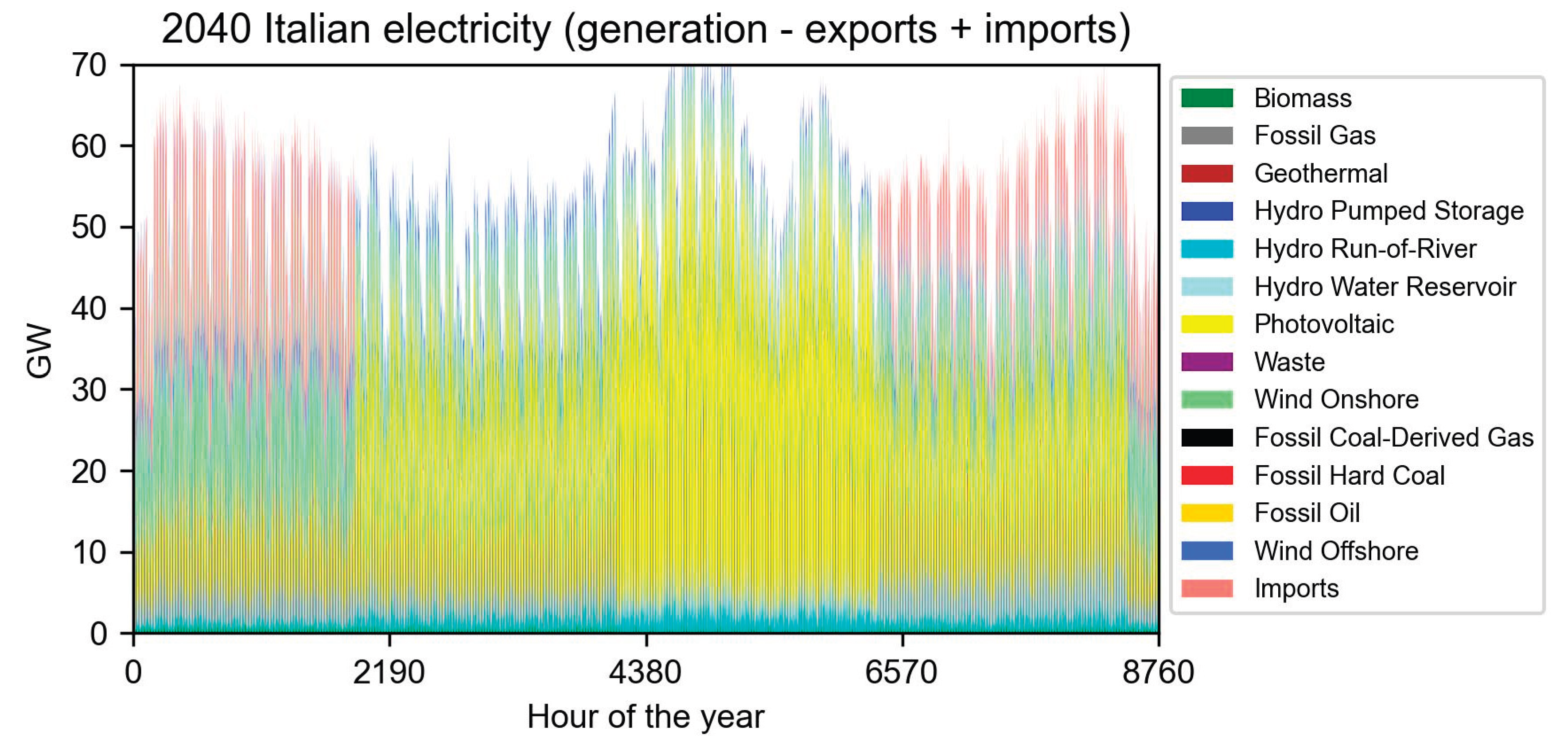
Between 2024 and 2040, the Italian electricity mix evolves according to the PNIEC and the Global Ambition scenario. Fossil fuel-based generation declines sharply, while solar and wind together exceed 50% of total electricity generation by 2040. Natural gas retains a strategic balancing role, particularly during periods of low renewable availability. Figure 6 presents the evolution of the Italian electricity grid composition from 2024 to 2040, obtained with OSeMOSYS.
Initially, one can see that year after year the accumulated demand keeps rising, as does the electricity generated by photovoltaic and wind power plants. In fact, the 2030-PNIEC foresees a doubling of current electricity transmission capacity across the territory, from 16 GW to more than 30 GW, necessary to meet forecasted demand growth in the years to come. On the same note, natural gas, as stated in the PNIEC, is crucial for grid stability because it provides a dispatchable, adjustable supply.
According to the graph, natural gas technology does not significantly reduce its contribution to electric energy production until 2030, when the widespread consolidation of PV and onshore wind occurs, along with the emergence of offshore wind. Other generation technologies, such as biomass, waste, geothermal, and all types of hydro, consistently supply the grid each year with a fixed share that remains aligned with the country's major environmental goals. From a cost perspective, the OSeMOSYS optimizer's solution did not include fossil oil. This is, anyhow, consistent with the official predictions and the recovered data from the base year, which indicate that less than 0.4 TWh of electricity was generated from this source. Figures A1–A3 present detailed load curves of electricity generation in Italy, including hourly contributions from the technologies.
Table 5 presents the static characterization outcomes obtained. As shown in the Table, all impact categories show lower burdens from 2024 to 2040, except for “human toxicity non-carcinogenic,” “land use,” and “material resources metals/minerals.” The reason for this trend is the production and installation of renewable energy plants, such as photovoltaics and wind turbines, which affect the 3 impact categories listed above, requiring large amounts of land to generate a significant volume of electric power (land use) and critical materials (material resources metals/minerals). In addition, the value chains of these activities in the ecoinvent library were most often in the global market; therefore, markets with high penetration of oil- or coal-fired power plants were also considered. These involve significant emission of non-carcinogenic toxic substances (i.e., metals and inorganics, i.e., solvents and industrial substances), compared to natural gas power-plant, such as heavy metals, CO, and NOₓ into the atmosphere. It should nevertheless be emphasized that this aspect requires further investigation, as a prospective background database is not employed (section 2.4). Moreover, it is well established in the scientific literature that the ecoinvent datasets for the production of photovoltaic modules and wind turbines are at least 10 years old [37,38].
The results for 2024, related to the climate change impact category, are in line with the electricity maps (based on TERNA data) and Italian Institute for Environmental Protection and Research (ISPRA) [39,40]: 255 vs. 274 and 215 (g CO2eq/kWhe), respectively. The variations are due to the system boundaries used to estimate the emission factors of the individual technologies serving the network. Compared with the result provided by ecoinvent, the value calculated in this work is lower, as ecoinvent presents, in its latest version (3.12), the value based on statistics from 2022. ISPRA reports highlight that the average national emission factor is decreasing over time, thanks to the growing share of energy from renewable sources and the decarbonization of the national electricity mix, i.e., from over 300 to 215 (g CO2-eq / kWhe) in 2024. This is confirmed using the present model on the 2022 database, yielding a value of 374 (g CO2eq / kWhe), in line with the reported order of magnitude by Naumann et al. (2024). To the best of the authors’ knowledge, there are no other scientific works in the literature related to the environmental profile of the current national electricity grid. Regarding 2030, the only publication is by Gargiulo et al. (2020). The authors estimate an emission factor for Italy of 226 g CO2-eq/kWhe. The value was based on the previous (2020) Integrated National Energy and Climate Plan (Piano Nazionale Integrato Energia e Clima – PNIEC) [39]. However, it provided for much lower renewable energy coverage than at present, i.e., 53% vs. 71%, respectively.
3.3. Evolution of Italian Electricity Profile (2024-2040)
This section presents the obtained hourly evolution from 2024 to 2040, illustrating the key statistical indicators. Namely, the average (), standard deviation (), and coefficient of variability (CV). These were calculated using the hourly values calculated for the individual years of the analysis. By doing so, this analysis provides both articulation and continuity with the previous assessments, allowing for a more comprehensive and coherent understanding of the model’s behavior and implications over time.
Figure 7a,b show a general temporal evolution for the climate change indicator. This impact (in 2024) is mainly driven by fossil fuels, with a CV of 23% and high values up to 255 kg CO2-eq/MWh, especially in the winter months. In 2040, the average value decreased, as expected, to 141 kg CO2-eq/MWh, thanks to the renewables with a consequent increase in the coefficient of variation (66% vs. 23%) and standard deviation (60 vs. 90 kg CO2-eq/MWh) compared to 2024, due to the discontinuity of renewables during the day (PV) and during the various months of the year (wind and PV).
Figure 7c,d show the behavior of acidification. Clearly, throughout 2024, this indicator is consistently above the 0.97 mol H+ eq/MWh (mean value), except in May, June, and July. In fact, during these late-spring and summer months, the impact on water acidification can go as low as 0.61 mol H+ eq/MWh. Fossil fuels, especially oil and hard coal, are the main emitters of these acidifying substances. Hence, it makes sense that, in summer, when photovoltaic and hydro power plants increase their production, this indicator falls to a sustained trough. The 20% for CV indicates significant variability in the data throughout the year. Also, for acidification, Figure 7d shows a lower mean value (with respect to 2024): 0.62 mol H+ eq/MWh vs. 0.97 mol H+ eq/MWh. In this case, however, a lower standard deviation (0.07 vs. 0.19 mol H+ eq/MWh) and a lower CV (11% vs. 20%) are presented compared to 2024. This is due to the non-use of coal and fuel oil sources in the electricity generation mix.
Figure 7e,f shows an evident influence of photovoltaic power plants and transmission of electricity over the exploitation of metals and minerals. In 2024, values up to 5.9 g Sbeq /MWh (max) are reached during the day in late spring and summer, while maintaining a minimum threshold of 3.8 g Sbeq /MWh throughout the nights all year long. In this case, as in the case of climate change, in 2040 it is presented an increase in the coefficient of variation (20% vs.11%) and standard deviation (1 vs. 0.5 g Sb eq/MWh) compared to 2024, due to the discontinuity of renewables during the day (PV) and during the various months of the year (wind and PV). The average value, on the other hand, increases with the high capacity of installed renewables (5.1 vs. 4.3 g Sbeq/MWh, respectively).
3.4. Applied Case Study: Positive Energy District
The previously presented results are applied within the urban energy sector. A simulated case study [40] that compares district system technologies with individual energy solutions was used to obtain an annual electricity consumption profile suitable for analyzing the results. The reported comparison was conducted for a new urban district planned for Bologna, Italy, covering approximately 41,000 m2 of heated and cooled floor area. To develop a more representative profile, one capable of showing the alternating dependence between the electrical grid and local self-generation for self-consumption, the following graphs are based on the resulting profile from a Fifth-Generation District Heating and Cooling (5GDHC) system that employs groundwater as a cold source and integrates 1.938 MWp of photovoltaic capacity. This configuration naturally defines a Positive Energy District, meaning it produces more final energy (i.e., electricity) than it consumes.
The 5GDHC concept is an advanced low-temperature district energy system that promotes bidirectional thermal exchange among interconnected buildings, enabling energy sharing, renewable integration, and simultaneous heating and cooling supply. These systems generally operate at (relatively low) temperatures below 40°C and are supported by central balancing units and seasonal storage that enhance overall energy flexibility. Such networks have proven highly effective in meeting the European Union’s climate and energy targets, particularly in new urban developments and urban regeneration projects.
Figure 8 presents the annual profile of the electricity produced on-site by the PV plant and exported to the national grid. There is a clear peak in electricity export of 900 kW, concentrated in the spring season, when solar resource availability is considerably higher than in winter and overall electricity demand is significantly lower. This pattern is not observed during the other transitional season, autumn, as higher electricity export costs limit the extent of exported generation during that period [40]. In fact, during summer and autumn, self-consumed electricity generated from the district’s own photovoltaic capacity covers the bulk of demand.
As discussed by several scientific articles, the carbon neutrality (a condition in which, during a specified period of time, the carbon footprint has been reduced, and if greater than zero, it is counterbalanced by offsetting) for buildings and districts is reached when the carbon footprint assessed by EN 15978 (at least at European level) is counterbalanced (net-balance approach) by the benefits of electricity exported to the national grid (presented in the Module D of the technical standard), plus, if it is necessary, by others options, i.e., insetting or economic compensations [41,42]. The aim of this section is precisely to discuss this approach by assessing the potential benefits of exporting electricity to the national grid using both average annual (static) emission factors and hourly (dynamic) emission factors.
Table 6 presents the results related to the operational Global Warming Potential (GWP) of the district, as introduced in the new Energy Performance of Buildings Directive (EPBD) [43], i.e., the emissions related to regulated loads of the buildings within the district, i.e., loads for heating and cooling, mechanical ventilation, transport, and artificial lighting. In addition, the Table presents the benefits of exporting the electricity produced by the on-site PV modules to the national grid and to non-regulated loads. The results shown in Table 6 are assessed using the following two equations.
where:
- is the electricity auto-consumed produced by PV at the hour (h).
- is the electricity auto-consumed supplied by the national grid at the hour (h).
- is the electricity exported produced by PV at the hour (h).
- is the emission factor of 1 kWh of electricity produced by PV (kgCO2eq/kWhe).
- is the emission factor of 1 kWh of electricity supplied by the grid at the hour (h) (kgCO2eq/kWhe). For static, the emission factor is considered as the arithmetical average of the dynamic emission factors of the years under evaluation (i.e., 2024 and 2040).
The results reported in the Table highlight two opposite outcomes: (i) negative net emissions—defined as the difference between the environmental benefit of exporting electricity and the operational GWP—when the static approach for 2024 is applied, and (ii) positive emissions for exporting electricity (i.e., no benefits) when the benefit is evaluated using the dynamic approach for 2040. It should be noted that electricity exports, which exceed the district’s local demand, exhibit a poorer environmental profile than the electricity from the national grid when the export occurs.
4. Discussion
The results of this study confirm that introducing an hourly temporal resolution in a prospective attributional LCA of electricity substantially enhances the interpretability of environmental impacts, particularly when the electricity system undergoes rapid structural changes driven by renewable energy penetration. The clustering of impact categories provides a useful framework to interpret both long-term trends and short-term variability, while the application to a Zero Emissions and Positive Energy District (ZEPED) demonstrates the practical relevance of time-resolved emission factors at the demand side.
4.1. Interpretation of Impact Category Clusters
Three main clusters of impact categories emerge from the analysis. The first cluster includes climate change plus non-renewable energy resources, particulate matter formation, photochemical oxidant formation, and ionizing radiation. These indicators show a clear and consistent reduction in annual average values between 2024 and 2040, reflecting the progressive phase-out of coal and oil and the declining role of natural gas in the Italian electricity mix. Although hourly variability increases for climate change impacts due to renewable intermittency, the overall downward trend confirms the effectiveness of the PNIEC-aligned decarbonization pathway. This behavior is consistent with previous dynamic LCA studies, but the present work highlights that variability itself becomes a defining feature of low-carbon electricity systems.
A second cluster comprises acidification, freshwater eutrophication, marine eutrophication, terrestrial eutrophication, and ozone depletion. These categories display both decreasing average impacts and reduced temporal variability over time. Their stabilization is largely attributable to the elimination of high-emitting fossil technologies and to the relatively steady contribution of hydroelectricity and imports. Unlike climate-related indicators, these categories benefit from a more homogeneous generation profile as fossil combustion processes are removed, making them less sensitive to hourly fluctuations in renewable output.
The third cluster includes land use, material resources (metals and minerals), human toxicity (non-carcinogenic), and water use. These categories show either increasing average values or, more importantly, a pronounced growth in temporal variability, reaching coefficients of variation close to 80% by 2040. This behavior is directly linked to the rapid deployment of photovoltaic and wind technologies, whose life-cycle impacts are dominated by infrastructure manufacturing, land occupation, and material extraction. The strong hourly variability observed for these categories highlights a structural trade-off of renewable-based systems: while operational emissions decline, upstream and spatially distributed burdens become more relevant. This result underscores the importance of considering non-climate indicators when evaluating long-term sustainability strategies and reinforces the need for improved, region-specific life cycle inventories for renewable technologies.
The clustering analysis demonstrates that relying solely on annual average emission factors can obscure critical dynamics. Categories in the first and third clusters, in particular, exhibit hourly patterns that may diverge significantly from annual means. As renewable penetration increases, hours with very low climate change intensity coexist with periods characterized by higher impacts due to imports or residual gas generation. This temporal heterogeneity is essential for informing demand-side strategies, grid management, and sector coupling policies.
Figure 9 provides the normalized variability of the impact categories investigated for 2024 (Figure 9a) and 2040 (Figure 9b). Equation No. 6 was used to normalize the results.
where:
- is the electricity supplied by the grid at the hour (h) of the year (j).
- is the emission factor of 1 kWh of electricity supplied by the grid at the hour (h) for the impact category (i) in the year (j).
- is the emission factor of 1 kWh of electricity supplied by the grid at the hour (h) for the impact category (i) in the year (j). For static, the emission factor is considered the arithmetic average of the dynamic emission factors for the years under evaluation (i.e., 2024 and 2040); thus, it is constant in the year of evaluation.
The land use impact stands out as the category that experiences the greatest reduction when analyzed on a time-specific basis. For both 2024 and 2040, the temporal impact analysis shows reductions of -83 and -82%, respectively, relative to the annual average. This finding highlights the environmental benefit of self-consumption through rooftop solar panels, which reduces grid electricity demand, particularly in summer when national photovoltaic generation peaks. In other words, during periods of abundant solar power production, this district relies less on grid electricity, thereby mitigating its overall land-use impacts.
4.2. Zero Emissions and Positive Energy District Case Study
A particularly relevant outcome concerns the comparison between exporting locally generated photovoltaic electricity and consuming electricity from the grid. By 2040, exporting PV electricity leads to an additional burden of approximately 11,000 kg CO₂-eq/year compared to consuming grid electricity during certain hours. This counterintuitive result highlights that, in highly decarbonized grids, exporting electricity during periods of low marginal impact may not always be environmentally optimal. Instead, maximizing self-consumption or shifting demand to hours with lower system-wide impacts can yield better environmental performance.
Overall, the ZEPED case study confirms that time-resolved LCA is a powerful decision-support tool for urban energy planning. It enables the identification of optimal consumption windows, supports the design of smart control strategies for heating, cooling, and mobility, and avoids misleading conclusions that may arise from static or averaged assessments.
From a policy and planning perspective, the results suggest that future decarbonization strategies should explicitly address impact-category trade-offs and temporal variability. While climate change mitigation remains central, increasing attention must be given to material use, land occupation, and toxicity-related impacts. Methodologically, the use of a prospective energy system model combined with a static background LCI represents a limitation, particularly for the third cluster of impacts. Incorporating prospective background databases could further refine the results and is identified as a priority for future research.
5. Conclusions
This study presented an attributional, prospective life cycle assessment of the Italian electricity grid over the period 2024–2040, using hourly emission factors derived from a cost-optimisation energy system model aligned with the Integrated National Climate and Energy Plan. The results confirm a profound transformation of the Italian electricity mix, characterized by the progressive phase-out of coal and oil, a declining but strategic role of natural gas, and a rapid expansion of solar photovoltaics and wind energy, which together exceed 50% of national electricity generation by 2040.
The environmental assessment, covering 16 impact categories, shows a consistent reduction in average impacts related to climate change, non-renewable energy use, particulate matter, and ionising radiation. At the same time, the increasing penetration of intermittent renewables leads to a marked rise in temporal variability for several indicators, particularly land use and material resource depletion. Based on their temporal behaviour, impact categories were grouped into three clusters, highlighting that decarbonisation reduces overall burdens but introduces new trade-offs linked to infrastructure intensity, land occupation, and critical material demand.
The analysis demonstrates that annual average emission factors are insufficient to capture these dynamics. Hourly resolution reveals pronounced intra-day and seasonal variations, especially in highly decarbonised scenarios, where periods of very low impacts coexist with hours dominated by imports or residual fossil generation. This temporal heterogeneity is crucial for demand-side optimisation, grid management, and policy design.
The application to a zero emissions and positive energy district in Bologna confirms the practical value of time-resolved emission factors. By 2040, the district achieves substantial reductions in several impact categories, notably land use (−82%) and ionising radiation (−40%), compared to the 2024 baseline. Importantly, the case study shows that exporting photovoltaic electricity to the grid may result in higher climate change impacts than consuming grid electricity during certain hours, leading to an additional burden of approximately 11,000 kg CO₂-eq in 2040. This counterintuitive result highlights the limitations of static, annual-average approaches and underscores the importance of maximising self-consumption and load shifting in future low-carbon grids.
Overall, this work demonstrates that high-resolution, prospective life cycle assessment method is essential for accurately assessing the environmental performance of rapidly evolving electricity systems. Future research should integrate prospective background databases, explicitly model energy storage, and expand system boundaries to include cross-sectoral interactions, thereby supporting more robust and informed decision-making for the energy transition.
Supplementary Materials
The following supporting information can be downloaded at the website of this paper posted on Preprints.org, Table S1: LCA results.
Author Contributions
For research articles with several authors, a short paragraph specifying their individual contributions must be provided. The following statements should be used "Conceptualization, J.D.C.C. and J.F.; methodology, J.D.C.C. and J.F.; software, J.D.C.C. and J.F.; validation, J.D.C.C., G.M., F.F. and J.F.; formal analysis, J.D.C.C.; investigation, J.D.C.C.; resources, J.D.C.C. and J.F.; data curation, J.D.C.C., G.M. and J.F; writing—original draft preparation, J.D.C.C. and J.F.; writing—review and editing, J.D.C.C., G.M., F.F. and J.F.; visualization, J.D.C.C. and J.F; supervision, J.F.; project administration, J.F.; funding acquisition, J.F. All authors have read and agreed to the published version of the manuscript.".
Funding
This research received no external funding.
Institutional Review Board Statement
Not applicable.
Informed Consent Statement
Not applicable.
Data Availability Statement
The original data presented in the study are openly available in Hourly-Attributional-Prospective-LCA-of-the-Italian-Electricity-Grid-from-2024-to-2040 at https://github.com/juandcortes17-rgb/Hourly-Attributional-Prospective-LCA-of-the-Italian-Electricity-Grid-from-2024-to-2040.
Conflicts of Interest
The authors declare no conflict of interest.
Declaration of generative AI in scientific writing
The authors declare that Grammarly was used exclusively to improve grammar, spelling, punctuation, and language clarity. The software did not generate scientific content, modify the meaning of the text, influence the research design, results, or interpretations, nor replace the authors’ intellectual contribution. All responsibility for the content of the manuscript remains with the authors.
Abbreviations
The following abbreviations are used in this manuscript:
| Ac | Acidification |
| CC | Climate Change |
| CCBio | Climate Change biogenic |
| CCF | Climate Change fossil |
| CCLU | Climate Change land use and land use change |
| CHP | Combined Heat and Power plant |
| Ecfw | Ecotoxicity − freshwater |
| EF | Environmental Footprint |
| EPBD | Energy Performance of Buildings Directive |
| ER | Energy Resources − non-renewable |
| EU | European Union |
| EUfw | Eutrophication − freshwater |
| Eum | Eutrophication − marine |
| Eut | Eutrophication − terrestrial |
| GWP | Global Warming Potential |
| HTc | Human Toxicity − carcinogenic |
| HTnc | Human Toxicity – non carcinogenic |
| IR | Ionizing Radiation |
| ISPRA | Italian Institute for Environmental Protection and Research |
| LCA | Life Cycle Assessment |
| LCI | Life Cycle Inventory |
| LU | Land Use |
| MASE | Ministry of Environment and Energy Security |
| MR | Material Resources − metals/minerals |
| MEF | Ministry of Economy and Finance |
| MIT | Ministry of Infrastructure and Transport |
| OD | Ozone Depletion |
| OSeMBE | Open-Source electricity Model Base for Europe |
| PM | Particulate Matter formation |
| PNIEC | Piano Nazionale Integrato Energia e Clima |
| POF | Photochemical Oxidant Formation |
| PV | Photovoltaic |
| TSO | Transmission System Operator |
| WU | Water Use |
| ZEPED | Zero Emissions and Positive Energy District |
Appendix A

Table A1.
Operational life and monetary costs of the different power plants [34].
Table A1.
Operational life and monetary costs of the different power plants [34].
| Generation technology | Power plant / Commodity (if present) |
Operational life (years) | CAPEX | OPEX | |||
|---|---|---|---|---|---|---|---|
| MUSD/GW | Fixed cost (MUSD /GW) |
Variable cost (MSUD/PJ) | |||||
| 2030 | 2040 | 2030 | 2040 | - | |||
| Photovoltaic | Utility scale | 25 | 706 | 571 | 12 | 10 | 0.0001 |
| Geothermal | Conventional geothermal |
40 | 3182 | 3084 | 64 | 62 | 0.0001 |
| Biomass | Biomass imports | 1 | - | - | - | - | 4.66 |
| Biomass extraction | 1 | - | - | - | - | 2.33 | |
| Combined cycle | 30 | 3127 | 2828 | 86 | 78 | 0.0084 | |
| CHP | 25 | 3155 | 3079 | 98 | 95 | 0.0001 | |
| Steam cycle | 30 | 1959 | 1914 | 72 | 70 | 0.0001 | |
| Fossil gas | Natural gas imports | 1 | - | - | - | - | 7.84 (2025) - 8.88 (2030-40) |
| Natural gas extraction | 1 | - | - | - | - | 7.05 (2025) - 7.99 (2030-40) | |
| Combined cycle | 30 | 826 | 826 | 21 | 21 | 0.0020 | |
| Gas cycle, new plant | 25 | 749 | 749 | 7 | 7 | 0.0133 | |
| Gas cycle, old plant | 25 | 535 | 535 | 16 | 16 | 0.0112 | |
| Heat and power, old plant | 25 | 876 | 876 | 86 | 86 | 0.0024 | |
| Heat and power, new plant | 25 | 985 | 976 | 45 | 44 | 0.0041 | |
| Internal combustion engine | 20 | 2017 | 2017 | 0 | 0 | 0.0150 | |
| Steam turbine | 30 | 1773 | 1773 | 56 | 56 | 0.0001 | |
| Fossil hard coal | Coal imports | 1 | - | - | - | - | 3.41 (2025) - 3.80 (2030-40) |
| Coal extraction | 1 | - | - | - | - | 3.07 (2025) - 3.42 (2030-40) | |
| Steam cycle, a big-sized plant | 30 | 1950 | 1950 | 61 | 61 | 0.0001 | |
| CHP | 25 | 1974 | 1974 | 0 | 0 | 0.0052 | |
| Fossil oil | Heavy fuel imports | 1 | - | - | - | - | 12.37 (2025) - 14.48 (2030-40) |
| Oil imports | 1 | - | - | - | - | 14.17 (2025) - 16.59 (2030-40) | |
| Oil extraction | 1 | - | - | - | - | 12.75 (2025) - 14.93 (2030-40) | |
| Gas cycle, new plant | 25 | 749 | 749 | 8 | 8 | 0.0133 | |
| Gas cycle, new plant | 25 | 535 | 535 | 16 | 16 | 0.0112 | |
| Internal combustion engine | 20 | 1313 | 1313 | 0 | 0 | 0.0001 | |
| Steam cycle, medium-sized plant | 30 | 1773 | 1773 | 56 | 56 | 0.0001 | |
| Steam cycle, big-sized plant | 30 | 1950 | 1950 | 61 | 61 | 0.0001 | |
| Waste | Waste extraction | 1 | - | - | - | - | 0.0001 |
| Combined heat and power | 25 | 5095 | 4735 | 191 | 178 | 0.0070 | |
| Steam cycle | 30 | 2304 | 2090 | 63 | 57 | 0.0036 | |
| Hydro pumped storage | Medium-sized plants | 80 | 2132 | 2132 | 75 | 75 | 0.0001 |
| Large-sized plants | 80 | 2513 | 2513 | 88 | 88 | 0.0001 | |
| Hydro run-of-river | “Small dams” | 80 | 3132 | 3122 | 125 | 125 | 0.0001 |
| Hydro water reservoir | Medium dams | 80 | 2132 | 2132 | 75 | 75 | 0.0001 |
| Large Dams | 80 | 2513 | 2513 | 88 | 88 | 0.0001 | |
| Wind offshore | Medium-and- Large -sized plants | 25 | 2743 | 2646 | 55 | 53 | 0.0001 |
| Wind onshore | Medium-and- Large -sized plants | 25 | 1240 | 1201 | 37 | 36 | 0.0001 |
Appendix B
Table A2.
Generation technologies considered in the Italian electricity mix LCA .
| Energy source (2024 ENTSO-E categories) and abbreviation | ecoinvent database specification (share %) | OSeMOSYS modelled technology (2025-2040 OSeMBE nomenclature) [34] |
|---|---|---|
| Photovoltaic | Electricity production, photovoltaic:
|
|
| Geothermal | Electricity production, deep geothermal | Geothermal conventional |
| Biomass | Heat and power co-generation:
|
|
| Fossil brown coal / lignite | Electricity production, lignite | - |
| Fossil coal-derived gas | Treatment of coal gas in power plant | - |
| Fossil gas | Electricity production, natural gas:
|
|
| Fossil hard coal (anthracite, coking coal and other bituminous coal) | Electricity production, hard coal (99%) Heat and power co-generation, hard coal (1%) |
|
| Fossil oil | Electricity production, oil (98%) Heat and power co-generation, oil (2%) |
|
| Waste | Electricity, from municipal waste incineration to generic market for electricity, medium voltage |
|
| Hydro pumped storage | Electricity production, hydro, pumped storage |
|
| Hydro run-of-river and poundage | Electricity production, hydro, run-of-river |
|
| Hydro water reservoir | Electricity production, hydro, reservoir, alpine region |
|
| Wind offshore | Electricity production, wind 1-3 MW turbine, offshore |
|
| Wind onshore |
|
|
Appendix C
Figure A1.
Electricity transmission profile for Italy in 2024 based on TERNA.
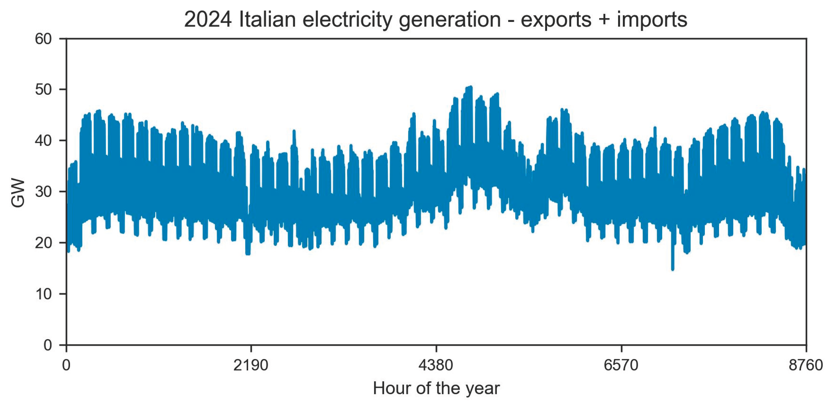
Table A3.
Daybreak and time slice used in the OSeMOSYS model.
| Season | Day break | Hour range | Time slice |
|---|---|---|---|
| Winter (S1) | S101 | 0:00-5:59 | 0.06 |
| S102 | 6:00-16:59 | 0.11 | |
| S103 | 17:00-24:00 | 0.07 | |
| Spring (S2) | S104 | 0:00-5:59 | 0.06 |
| S105 | 6:00-16:59 | 0.13 | |
| S106 | 17:00-24:00 | 0.06 | |
| Summer (S3) | S107 | 0:00-5:59 | 0.05 |
| S108 | 6:00-16:59 | 0.17 | |
| S109 | 17:00-24:00 | 0.03 | |
| Autumn (S4) | S110 | 0:00-5:59 | 0.06 |
| S111 | 6:00-16:59 | 0.13 | |
| S112 | 17:00-24:00 | 0.05 |
Table A4.
Specified electricity demand profile and capacity factors for solar, hydro, and wind sources.
Table A4.
Specified electricity demand profile and capacity factors for solar, hydro, and wind sources.
| Day break | Specified demand profile | Capacity factor (value from 0 to 1) | |||
|---|---|---|---|---|---|
| Solar | Hydro (reservoir and pump and storge) | Hydro (run-of-river) | Wind | ||
| S101 | 0.05 | 0.0000 | 0.12 | 0.23 | 0.42 |
| S102 | 0.12 | 0.1000 | 0.29 | 0.33 | 0.42 |
| S103 | 0.08 | 0.0000 | 0.39 | 0.41 | 0.42 |
| S104 | 0.05 | 0.0001 | 0.34 | 0.54 | 0.27 |
| S105 | 0.13 | 0.3000 | 0.41 | 0.57 | 0.31 |
| S106 | 0.06 | 0.0200 | 0.56 | 0.67 | 0.31 |
| S107 | 0.05 | 0.0042 | 0.42 | 0.48 | 0.16 |
| S108 | 0.20 | 0.4000 | 0.50 | 0.55 | 0.21 |
| S109 | 0.03 | 0.0000 | 0.57 | 0.60 | 0.16 |
| S110 | 0.05 | 0.0032 | 0.22 | 0.34 | 0.28 |
| S111 | 0.15 | 0.2500 | 0.39 | 0.45 | 0.29 |
| S112 | 0.04 | 0.0000 | 0.38 | 0.45 | 0.29 |
|
Additional (manual) modelling choices: Capacity Factor for electricity imports was set to 0.6 for S102, S105, S108, and S111. For the remaining day breaks this parameter was set to 0. The OSeMOSYS parameter "TotalTechnologyAnnualActivityUpperLimit" was left unconstrained (i.e. 99999 PJ) for Hydro run-of-river and Hydro Pump and Storage. | |||||
Appendix D
Figure A2.
Italian 2024 net electricity mix.
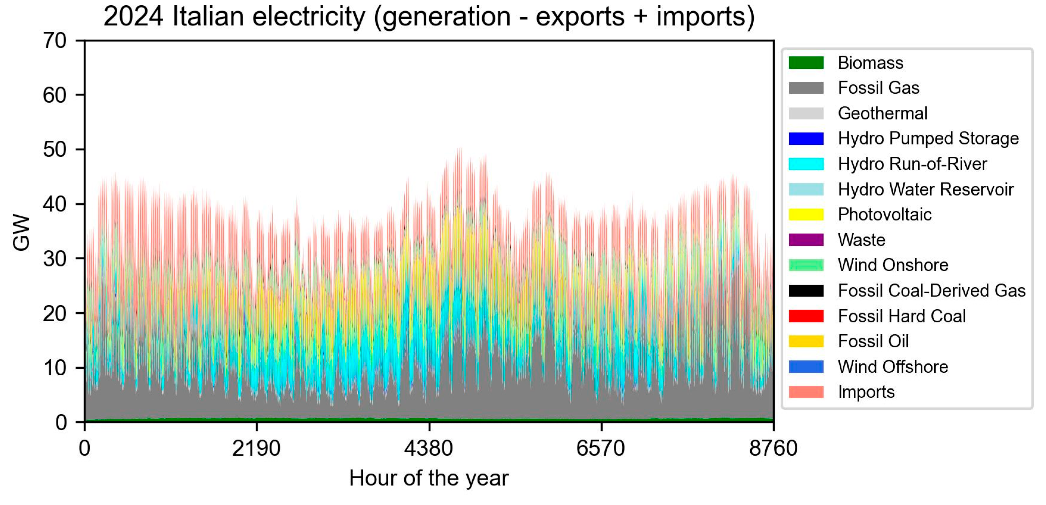
Figure A3.
Italian 2030 net electricity mix.
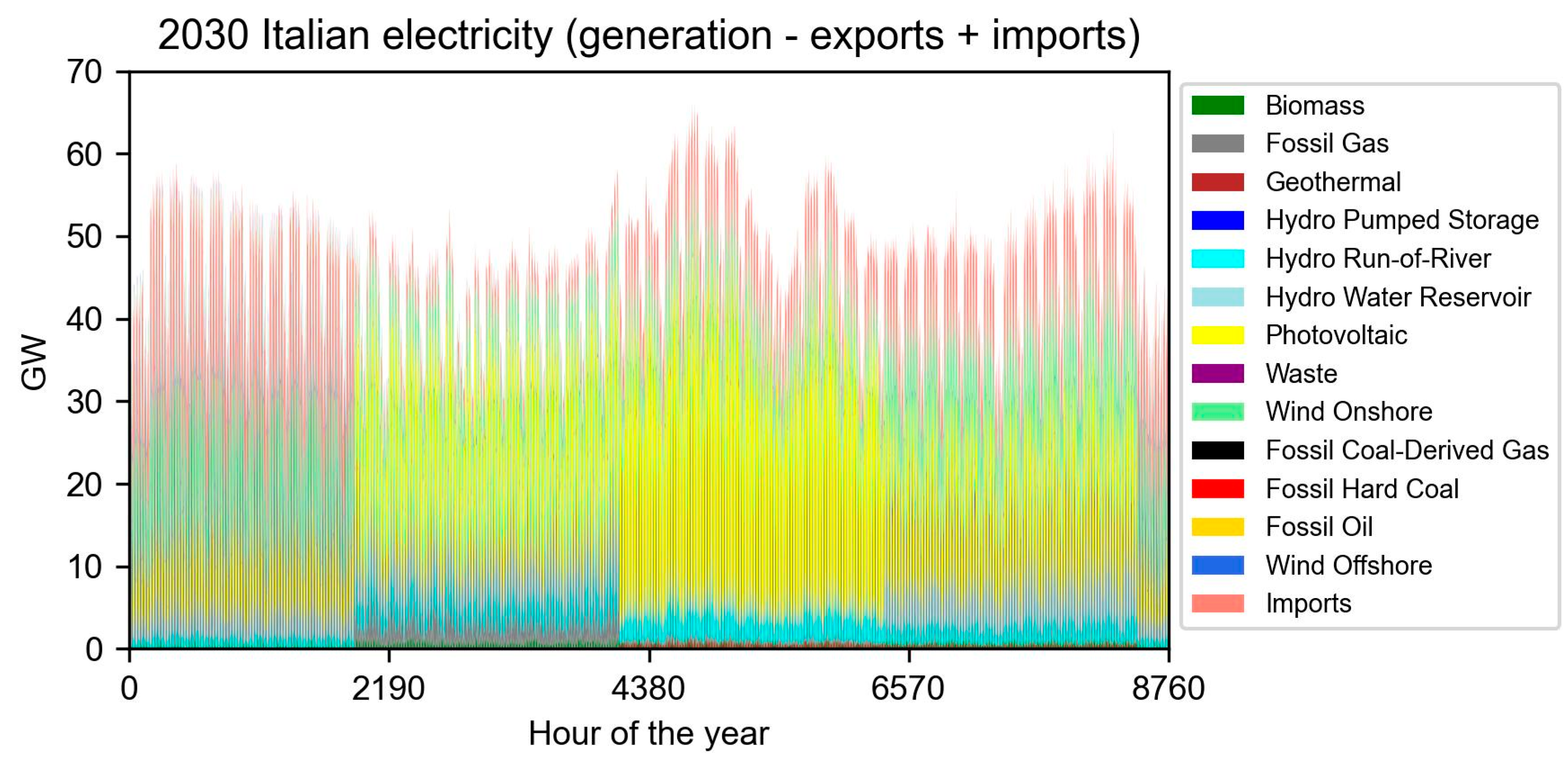
Figure A4.
Italian 2040 net electricity mix.
References
- Eyring, V.; Gillett, N.P.; Achuta Rao, K.M.; Barimalala, R.; Barreiro Parrillo, M.; Bellouin, N.; Cassou, C.; Durack, P.J.; Kosaka, Y.; McGregor, S.; et al. Human Influence on the Climate System. In Climate Change 2021: The Physical Science Basis. Contribution of Working Group I to the Sixth Assessment Report of the I. In Climate Change 2021: The Physical Science Basis. Contribution of Working Group I to the Sixth Assessment Report of the Intergovernmental Panel on Climate Change; Masson-Delmotte, V., Zhai, P., Pirani, A., Connors, S. L., Péan, C., Berger, S., Zhou, B., Eds.; Cambridge University Press, 2023; pp. 423–552. [Google Scholar]
- Doan, N.; Doan, H.; Nguyen, C.P.; Nguyen, B.Q. From Kyoto to Paris and beyond: A Deep Dive into the Green Shift. Renew. Energy 2024, 228, 120675. [Google Scholar] [CrossRef]
- Robertson, G.L. Packaging and Food and Beverage Shelf Life. In The Stability and Shelf Life of Food; Elsevier, 2016; pp. 77–106. [Google Scholar]
- Nieuwlaar, E. Life Cycle Assessment and Energy Systems. In Reference Module in Earth Systems and Environmental Sciences; Elsevier, 2013. [Google Scholar]
- ISO ISO 14040:2006+A1:2020; Environmental Management — Life Cycle Assessment — Principles and Framework. 2020; pp. 1–30.
- ISO ISO 14044:2006+A2:2020: Environmental Management - Life Cycle Assessment - Requirements and Guidelines; 2020; pp. 1–64.
- Finocchi, E. Electricity as an Energy Vector: A Performance Comparison with Hydrogen and Biodiesel in Italy. Open J. Energy Effic. 2024, 13, 1–24. [Google Scholar] [CrossRef]
- Weidema, B.P. Market Information in LCA. Environmental Project No. 863.
- Arvidsson, R.; Tillman, A.; Sandén, B.A.; Janssen, M.; Nordelöf, A.; Kushnir, D.; Molander, S. Environmental Assessment of Emerging Technologies: Recommendations for Prospective LCA. J. Ind. Ecol. 2018, 22, 1286–1294. [Google Scholar] [CrossRef]
- TERNA, S.p.A. Generation Statistical Data. Available online: https://dati.terna.it/en/generation/statistical-data#capacity/generation-plants (accessed on 5th of April 2025).
- MASE Piano Nazionale Integrato per l’Energia e Il Clima 2030. Available online: https://www.mase.gov.it/portale/documents/d/guest/pniec_2024_revfin_01072024-errata-corrige-pulito-pdf (accessed on 5 April 2025).
- Gargiulo, A.; Carvalho, M.L.; Girardi, P. Life Cycle Assessment of Italian Electricity Scenarios to 2030. Energies 2020, 13, 3852. [Google Scholar] [CrossRef]
- Carvalho, M.L.; Marmiroli, B.; Girardi, P. Life Cycle Assessment of Italian Electricity Production and Comparison with the European Context. Energy Reports 2022, 8, 561–568. [Google Scholar] [CrossRef]
- European Commission EUROSTAT Database. Available online: https://ec.europa.eu/eurostat/data/database (accessed on 4th of May 2025).
- Wernet, G.; Bauer, C.; Steubing, B.; Reinhard, J.; Moreno-Ruiz, E.; Weidema, B. The Ecoinvent Database Version 3 (Part I): Overview and Methodology. Int. J. Life Cycle Assess. 2016, 21, 1218–1230. [Google Scholar] [CrossRef]
- Bastos, J.; Prina, M.G.; Garcia, R. Life-Cycle Assessment of Current and Future Electricity Supply Addressing Average and Marginal Hourly Demand: An Application to Italy. J. Clean. Prod. 2023, 399, 136563. [Google Scholar] [CrossRef]
- Peters, P.; da Costa, V.B.F.; Dias, B.H.; Bonatto, B.D. A Holistic Analysis of Environmental Impacts and Improvement Pathways for the Brazilian Electric Sector Based on Long-Term Planning and Life Cycle Assessment. Appl. Energy 2025, 377, 124505. [Google Scholar] [CrossRef]
- Messagie, M.; Mertens, J.; Oliveira, L.; Rangaraju, S.; Sanfelix, J.; Coosemans, T.; Van Mierlo, J.; Macharis, C. The Hourly Life Cycle Carbon Footprint of Electricity Generation in Belgium, Bringing a Temporal Resolution in Life Cycle Assessment. Appl. Energy 2014, 134, 469–476. [Google Scholar] [CrossRef]
- Barros, M.V.; Salvador, R.; Piekarski, C.M.; de Francisco, A.C.; Freire, F.M.C.S. Life Cycle Assessment of Electricity Generation: A Review of the Characteristics of Existing Literature. Int. J. Life Cycle Assess. 2020, 25, 36–54. [Google Scholar] [CrossRef]
- Howells, M.; Rogner, H.; Strachan, N.; Heaps, C.; Huntington, H.; Kypreos, S.; Hughes, A.; Silveira, S.; DeCarolis, J.; Bazillian, M.; et al. OSeMOSYS: The Open Source Energy Modeling System. Energy Policy 2011, 39, 5850–5870. [Google Scholar] [CrossRef]
- Gardumi, F.; Shivakumar, A.; Morrison, R.; Taliotis, C.; Broad, O.; Beltramo, A.; Sridharan, V.; Howells, M.; Hörsch, J.; Niet, T.; et al. From the Development of an Open-Source Energy Modelling Tool to Its Application and the Creation of Communities of Practice: The Example of OSeMOSYS. Energy Strateg. Rev. 2018, 20, 209–228. [Google Scholar] [CrossRef]
- Niet, T.; Shivakumar, A.; Gardumi, F.; Usher, W.; Williams, E.; Howells, M. Developing a Community of Practice around an Open Source Energy Modelling Tool. Energy Strateg. Rev. 2021, 35, 100650. [Google Scholar] [CrossRef]
- SNAM; TERNA Documento Di Descrizione Degli Scenari 2024. Available online: https://download.terna.it/terna/Documento_Descrizione_Scenari_2024_8dce2430d44d101.pdf (accessed on 5th of May 2025).
- Villa, G.; Famiglietti, J.; Dénarié, A.; Aprile, M.; Motta, M. Life Cycle Cost Assessment of a Positive Energy District Featuring a 5th-Generation Heating and Cooling Network: An Italian Residential and Light Commercial Case Study. Energy Build. 2025, 347, 116299. [Google Scholar] [CrossRef]
- Naumann, G.; Famiglietti, J.; Schropp, E.; Motta, M.; Gaderer, M. Dynamic Life Cycle Assessment of European Electricity Generation Based on a Retrospective Approach. Energy Convers. Manag. 2024, 311, 118520. [Google Scholar] [CrossRef]
- Fazio, S.; Castellani, V.; Sala, S.; Schau, E.M.; Secchi, M.; Zampori, L.; Diaconu, E. Supporting Information to the Characterisation Factors of Recommended EF Life Cycle Impact Assessment Method; 2018; ISBN 9789279767425. [Google Scholar]
- TERNA Download Center. Available online: https://dati.terna.it/download-center (accessed on the 4th of May 2025).
- ENTSO-E The ENTSO-E Transparency Platform. Available online: https://www.entsoe.eu/data/transparency-platform/ (accessed on 5th of May 2025).
- Sacchi, R.; Terlouw, T.; Siala, K.; Dirnaichner, A.; Bauer, C.; Cox, B.; Mutel, C.; Daioglou, V.; Luderer, G. PRospective EnvironMental Impact AsSEment (Premise): A Streamlined Approach to Producing Databases for Prospective Life Cycle Assessment Using Integrated Assessment Models. Renew. Sustain. Energy Rev. 2022, 160, 112311. [Google Scholar] [CrossRef]
- de Wet, N.; Mohanty, R.; Cannone, C.; Kell, A.; Buzzlightyear; Usher, W. ClimateCompatibleGrowth/ClicSAND: ClicSAND. Available online: https://github.com/OSeMOSYS/clicSAND (accessed on 10th of September 2025).
- Plazas Niño, F.; Kapor, V.; Tan, N. Modelling User Interface for OSeMOSYS (MUIO). Available online: https://github.com/OSeMOSYS/MUIO (accessed on 10th of September 2025).
- Trinh, B.; Phong, N.V. 2013. A Short Note on RAS. Method. Available online: https://github.com/OSeMOSYS/MUIO (accessed on 9th of May 2025).
- European Commission EU Reference Scenario 2020. Available online: https://energy.ec.europa.eu/data-and-analysis/energy-modelling/eu-reference-scenario-2020_en.
- Henke, H.T.J.; Gardumi, F.; Howells, M. The Open Source Electricity Model Base for Europe - An Engagement Framework for Open and Transparent European Energy Modelling. Energy 2022, 239, 121973. [Google Scholar] [CrossRef]
- Schwarz, M.; Renggli, S.; Gjorgiev, B.; Garrison, J. Swiss Electricity Supply after the “Mantelerlass” – Quo Vadis? A Perspective on Nuclear Power. Available online: https://nexus-e.org/role-of-nuclear-power/ (accessed on 5th of July 2025).
- IEA - International Energy Agency The Role of Critical Minerals in Clean Energy Transitions. Available online: https://www.iea.org/reports/the-role-of-critical-minerals-in-clean-energy-transitions (accessed on 9th of October 2025).
- Kolahchian Tabrizi, M.; Famiglietti, J.; Bonalumi, D.; Campanari, S. How the Boundaries of the Supply Chain Affect Climate Profile: The Case of Renewable Electricity and Green Hydrogen for Italy and the UK. Int. J. Hydrogen Energy 2025, 106, 156–170. [Google Scholar] [CrossRef]
- Tabrizi, M.K.; Famiglietti, J.; Bonalumi, D.; Campanari, S. The Carbon Footprint of Hydrogen Produced with State-of-the-Art Photovoltaic Electricity Using Life Cycle Assessment Methodology. Energies 2023, 16, 5190. [Google Scholar] [CrossRef]
- MASE Piano Nazionale Integrato per l’Energia e Il Clima. Available online: https://www.mase.gov.it/portale/documents/d/guest/pniec_finale_17012020-pdf (accessed on 12 December 2025).
- Famiglietti, J.; Villa, G.; Romagnosi, M.; Dénarié, A.; Scoccia, R.; Motta, M. Net Zero Emissions and Positive Energy Districts: A Potential Solution to Achieve the European Climate Targets. In Proceedings of the 2024 IEEE International Conference on Environment and Electrical Engineering and 2024 IEEE Industrial and Commercial Power Systems Europe (EEEIC / I&CPS Europe), 17th of June 2024; IEEE; pp. 1–6. [Google Scholar]
- Famiglietti, J.; Aprile, M.; Spirito, G.; Motta, M. Net-Zero Climate Emissions Districts: Potentials and Constraints for Social Housing in Milan. Energies 2023, 16. [Google Scholar] [CrossRef]
- Lützkendorf, T.; Frischknecht, R. (Net-) Zero-Emission Buildings: A Typology of Terms and Definitions. Build. Cities 2020, 1, 662–675. [Google Scholar] [CrossRef]
- European Parliament and Council Directive (EU) 2024/1275 of the European Parliament and of the Council of the 24th of April 2024 on the Energy Performance of Buildings (Recast); European Union, 2024; p. 68.
Figure 1.
General outline of system boundary.
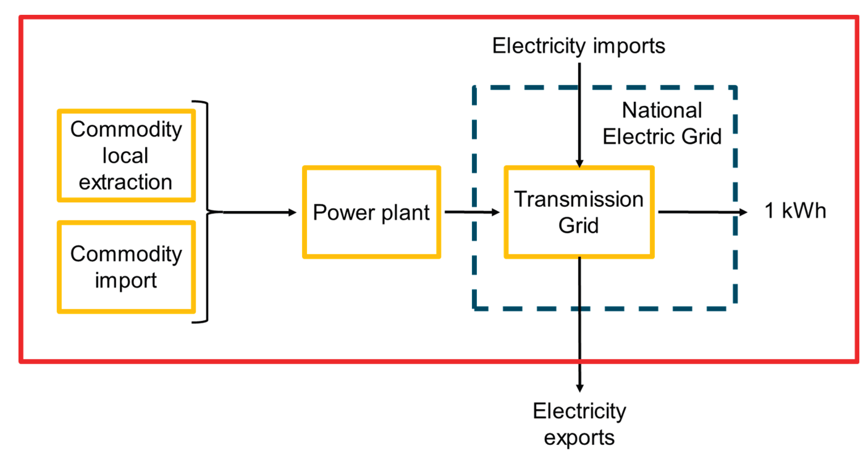
Figure 2.
Summary scheme of the base year model.
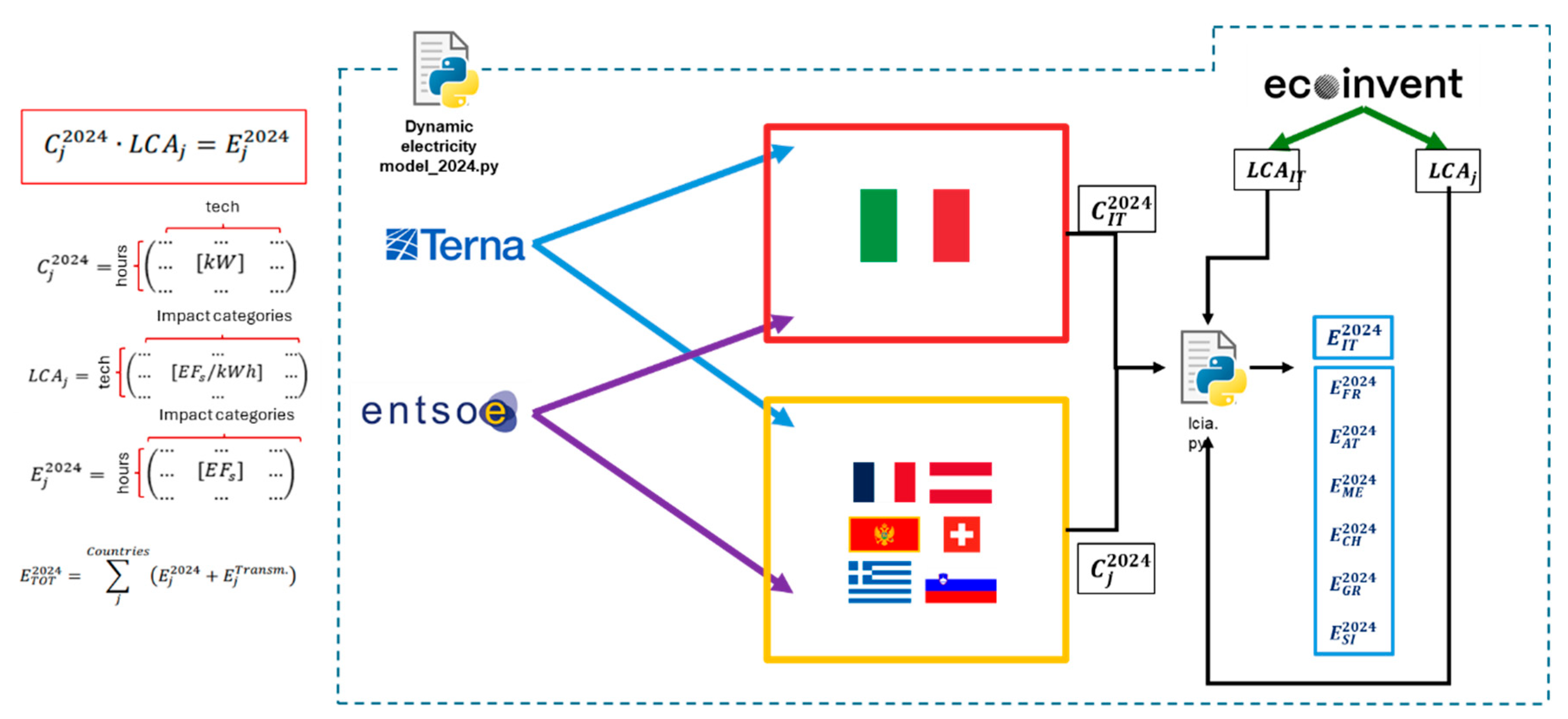
Figure 3.
Summary scheme of the 2025-2040 model.
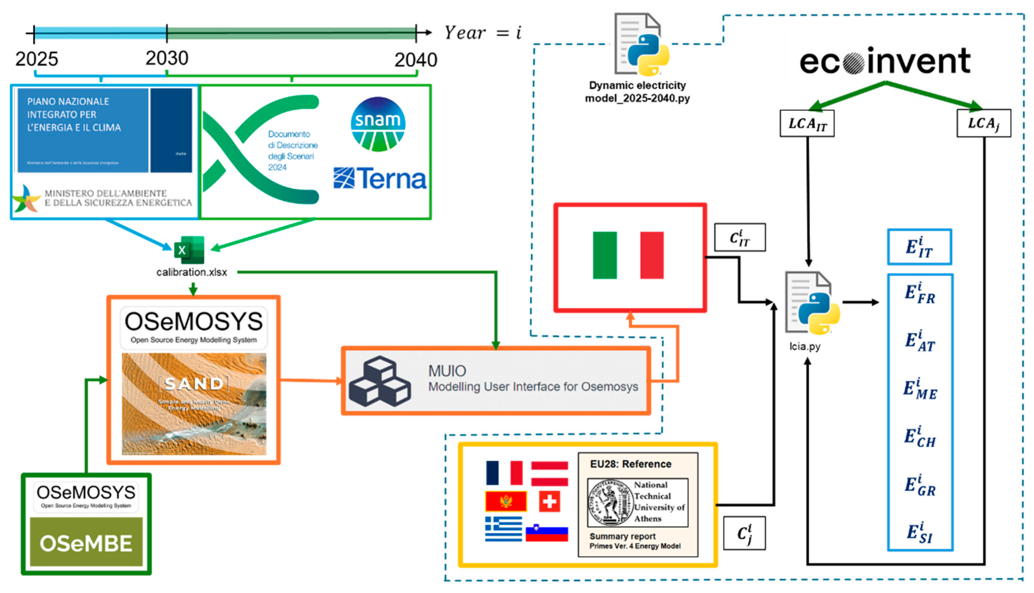
Figure 4.
Italian electricity imports 2024, relative contribution per country.
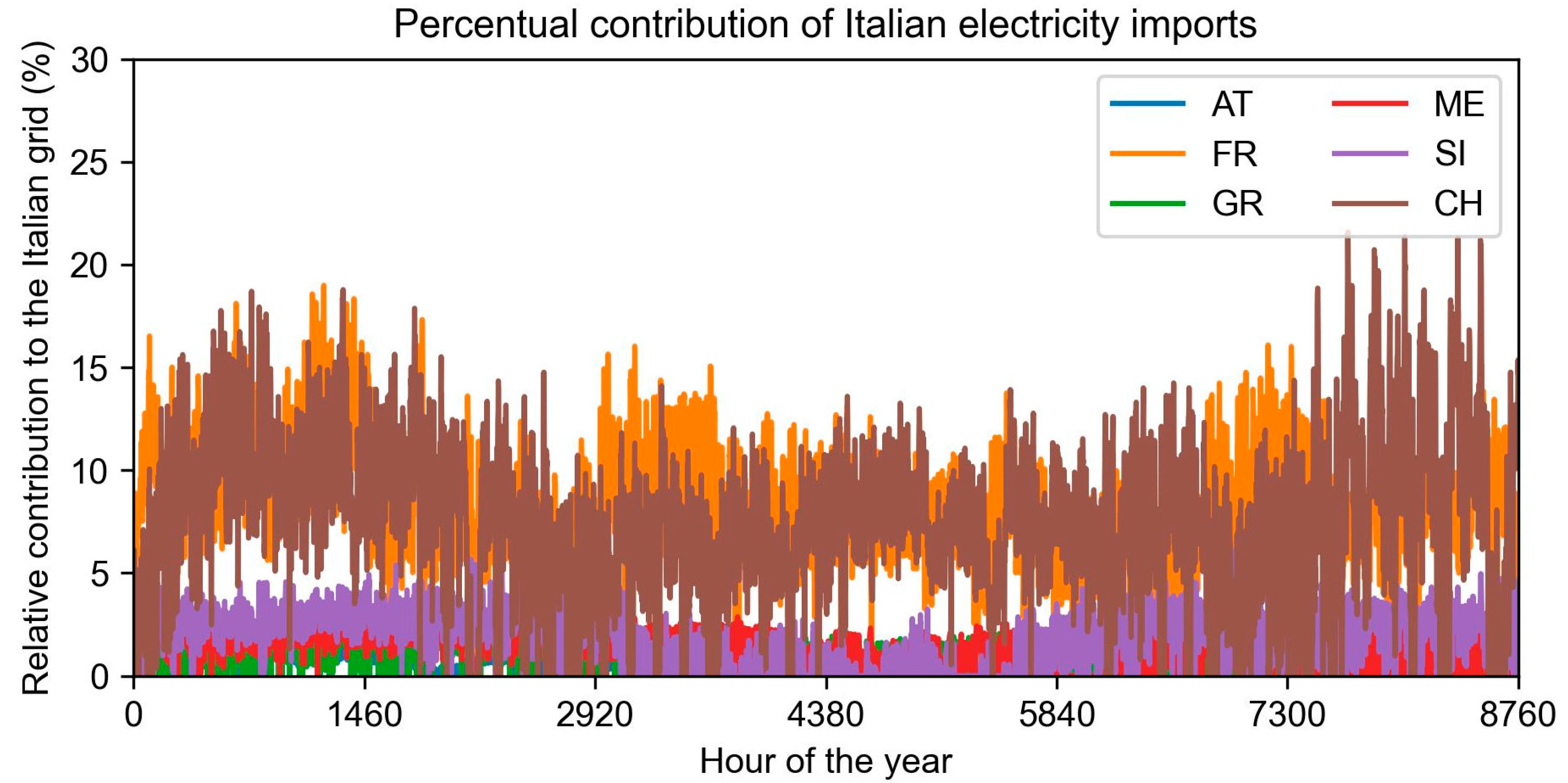
Figure 5.
(a) Climate change, (b) acidification, and (c) material resources: metals/minerals outcomes per energy source in Italy.
Figure 5.
(a) Climate change, (b) acidification, and (c) material resources: metals/minerals outcomes per energy source in Italy.
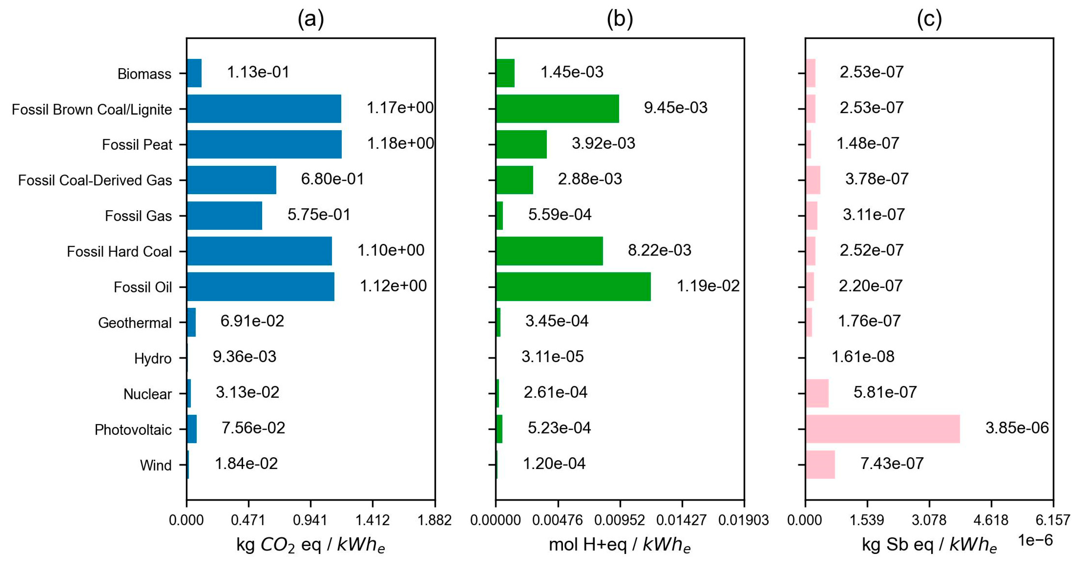
Figure 6.
Evolution of the Italian electricity grid composition 2024-2040, obtained with OSeMOSYS.
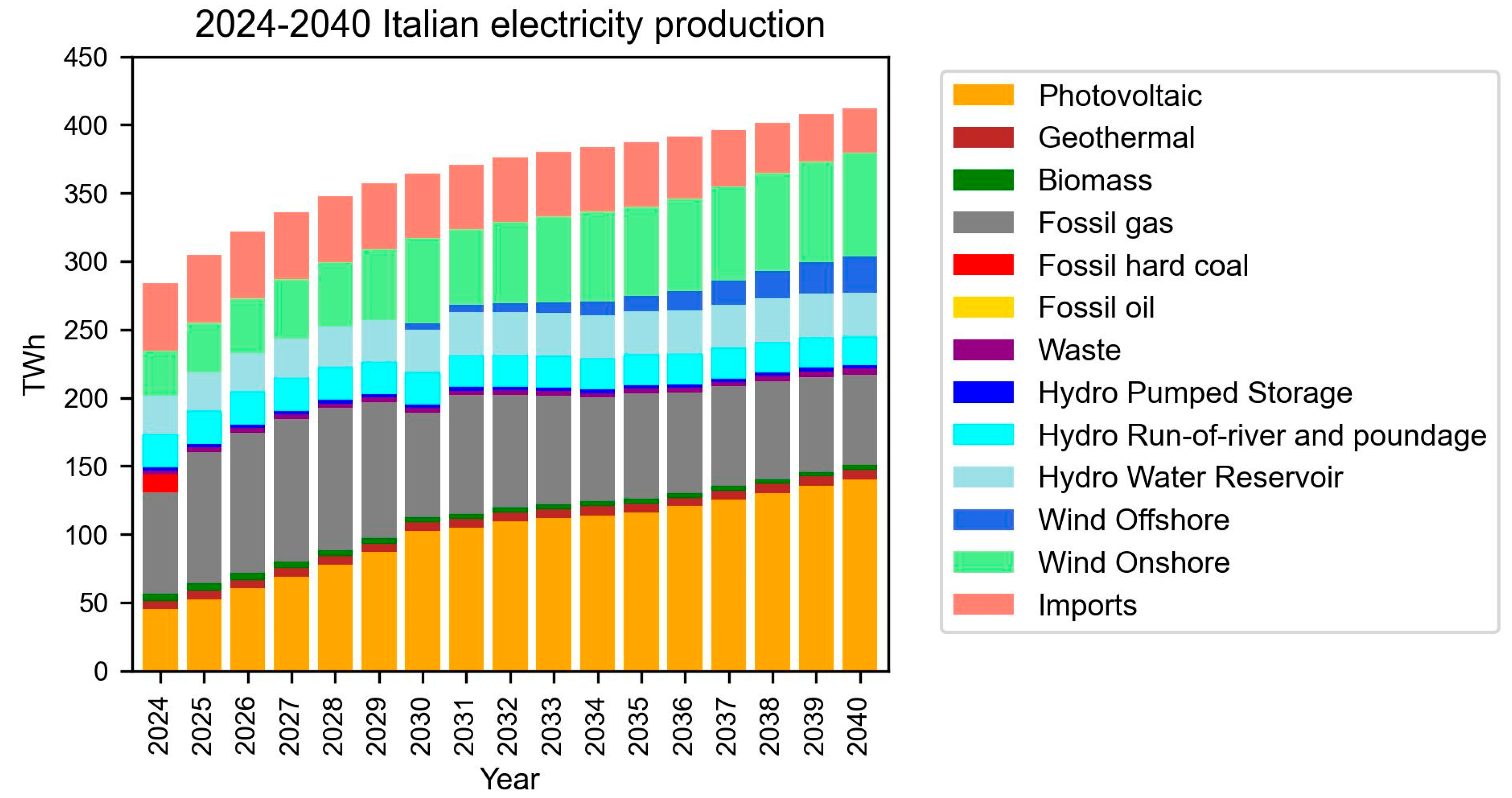
Figure 7.
Coefficient of Variation (CV) for (a) climate change in 2024, (b) climate change in 2040, (c) acidification in 2024, (d) acidification in 2040, (e) material resources: metals/minerals in 2024, and (f) material resources: metals/minerals in 2040.
Figure 7.
Coefficient of Variation (CV) for (a) climate change in 2024, (b) climate change in 2040, (c) acidification in 2024, (d) acidification in 2040, (e) material resources: metals/minerals in 2024, and (f) material resources: metals/minerals in 2040.
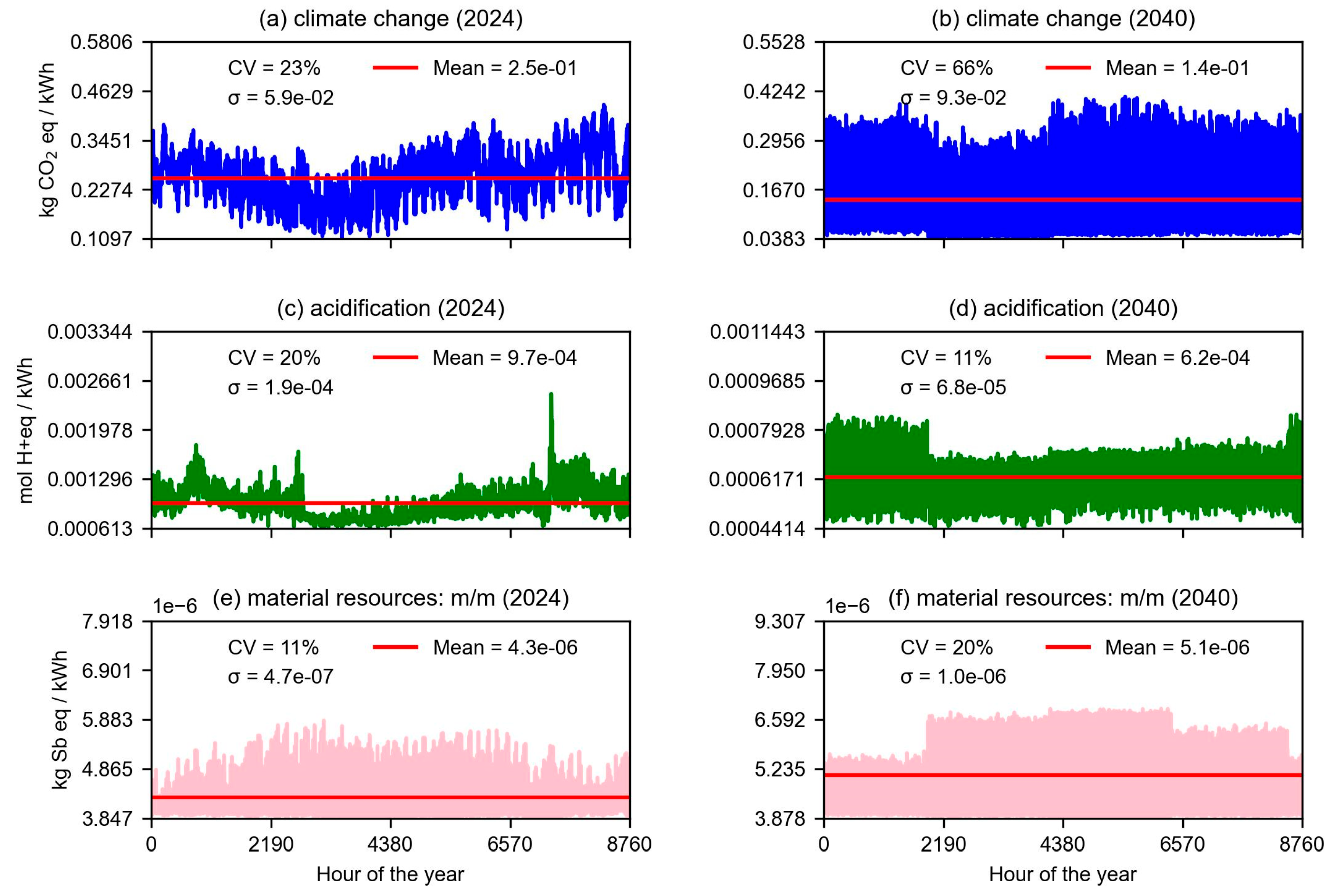
Figure 8.
Electricity exported to the national grid.
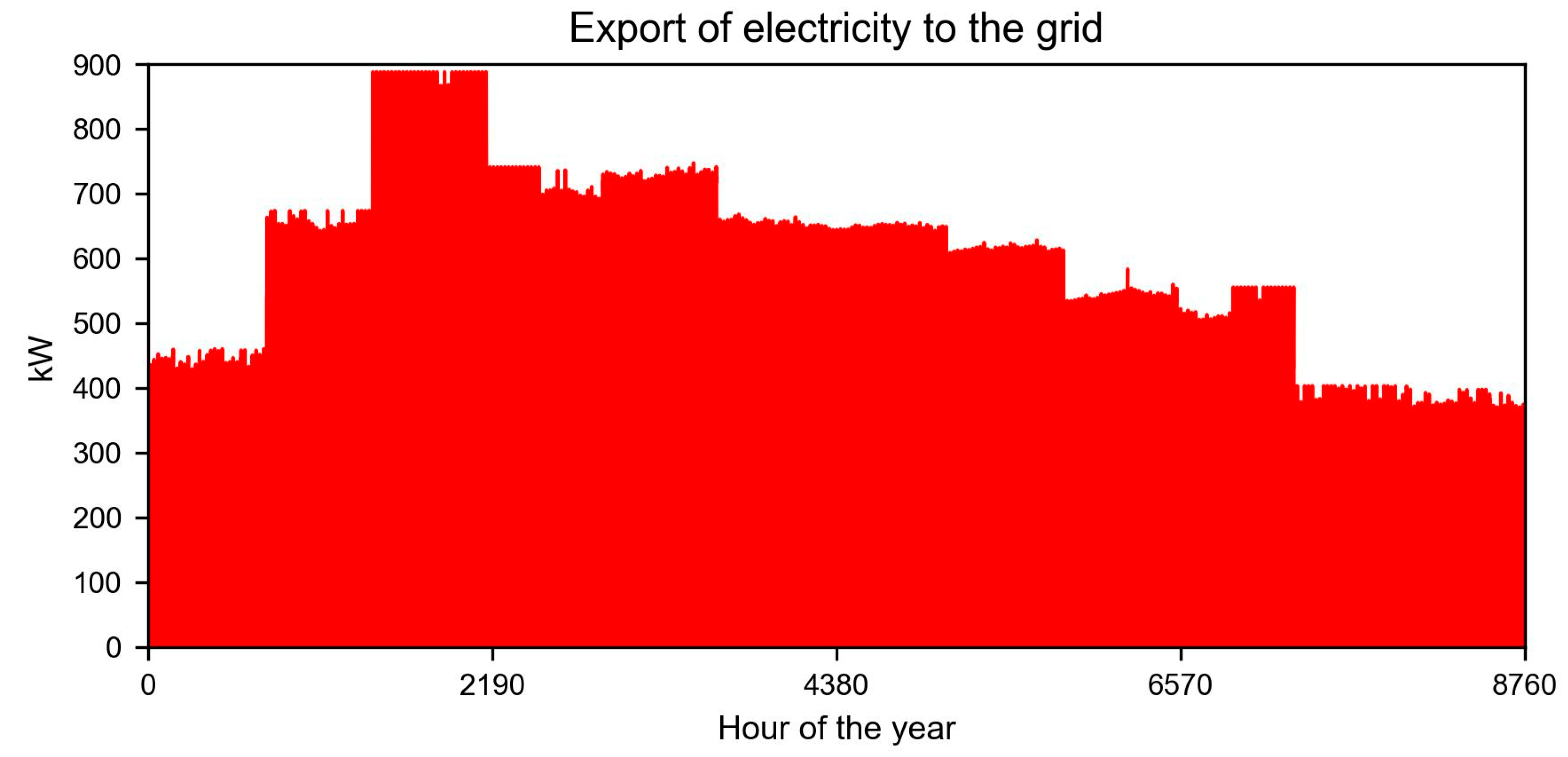
Figure 9.
Normalized variability of all impact categories in (a) 2024 and (b) 2040.
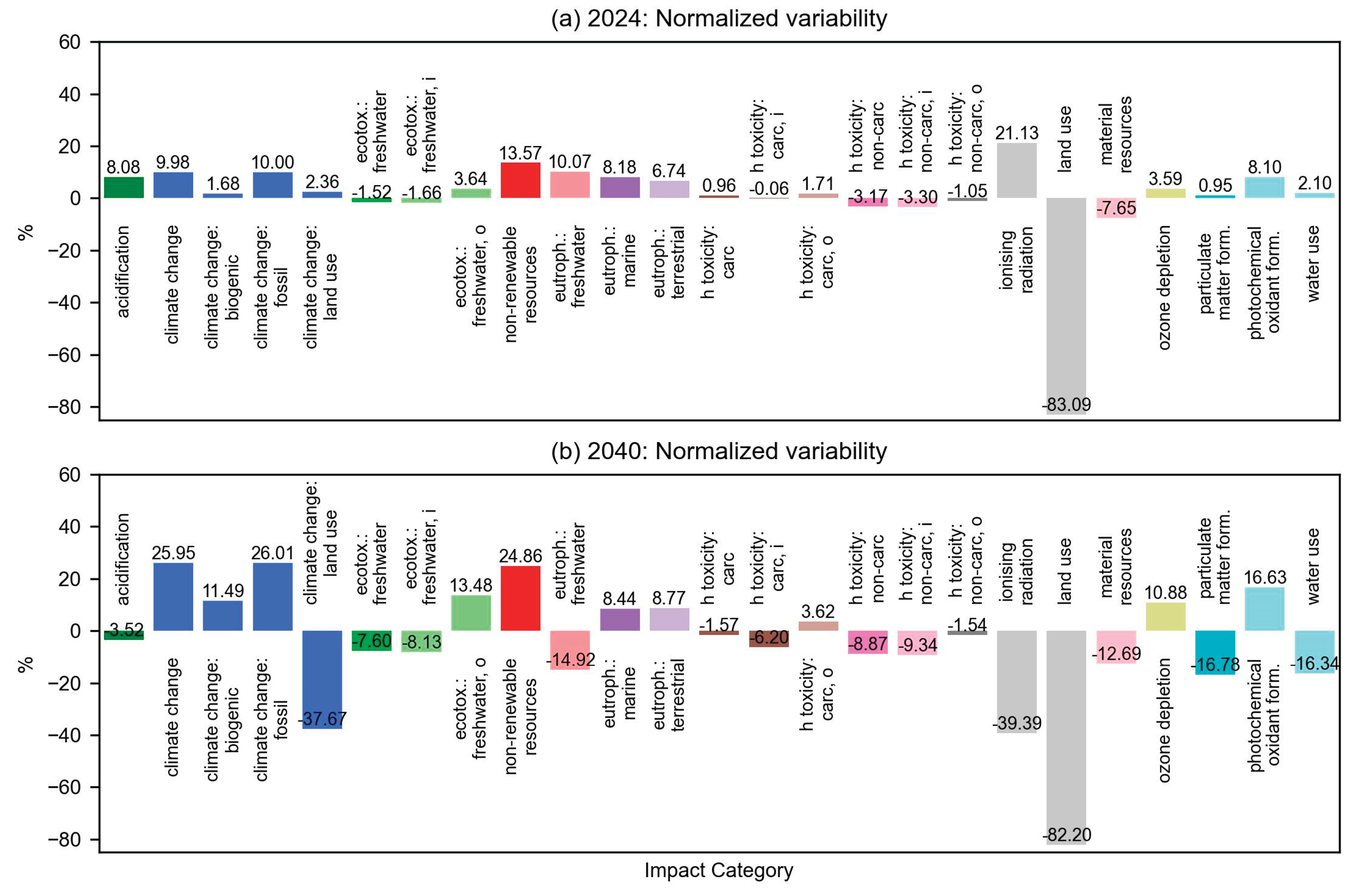
Table 1.
Current and residual capacities for each of the technologies modelled in OSeMOSYS.
| Technology | 2024 (GW) | 2030 (GW) | 2040 (GW) |
|---|---|---|---|
| Hydropower | 19.0 | 19.4 | 19.4 |
| Wind onshore | 13.0 | 28.1 | 29.0 |
| Wind offshore | 0.0 | 2.1 | 10.0 |
| Geothermal | 0.8 | 1.0 | 1.5 |
| Solar | 37.0 | 79.3 | 105.1 |
| Biomass | 4.0 | 3.2 | 1.6 |
| Thermoelectric | 58.3 | 54.4 | 47.6 |
Table 2.
Current annual electricity generation and future objectives in Italy.
| Energy source | 2024 (TWh) |
2030 PNIEC (TWh) |
Global ambition (TWh) |
||
|---|---|---|---|---|---|
| 2030 | 2035 | 2040 | |||
| Electricity demand | 293 | 362 | 385 | 415 | |
| Hydrpower | 53.3 | 47 | 46 | 46 | |
| Geothermal | 4.8 | 6 | 7 | 7 | |
| Wind | 22.0 | 64 | 79 | 105 | |
| Biomass | 5.2 | 11 | 10 | 10 | |
| Waste | 2.9 | 3 | 4 | 4 | |
| Solar | 27.9 | 105 | 127 | 151 | |
| Natural gas | 94.6 | 93 | 83 | 64 | |
| Oil | 1.09 | 0.2 | 0 | 0 | |
| Coal | 8.4 | 0 | 0 | 0 | |
| Net imports | 52 | 43 | 47 | 46 | |
| Energy storage capacities | 0.0 | 0.122 | 0.137 | 0.184 | |
Table 3.
Assumed fixed percentage distribution of imported electricity in Italy 2024-2040.
| Country | 2024 electricity imported by Italy (TWh) | Share (%) |
|---|---|---|
| France | 21.7 | 39.7 |
| Switzerland | 20.8 | 38.2 |
| Slovenia | 4.9 | 8.9 |
| Montenegro | 3.2 | 5.9 |
| Greece | 2.5 | 4.6 |
| Austria | 1.5 | 2.7 |
Table 4.
Year split used in the OSeMOSYS model.
| Season | Start day number | End day number | Start date | End date | Start/end hour | No. of days |
|---|---|---|---|---|---|---|
| Winter (S1) | 1 | 79 | 1-Jan | 20-Mar | 0-1896 | 79 |
| Spring (S2) | 80 | 172 | 21-Mar | 21-Jun | 1897-4128 | 93 |
| Summer (S3) | 173 | 265 | 22-Jun | 22-Sep | 4129-6360 | 93 |
| Autumn (S4) | 266 | 354 | 23-Sep | 20-Dec | 6361-8496 | 89 |
| Winter (S1) | 355 | 365 | 21-Dec | 31-Dec | 8497-8760 | 11 |
Table 5.
Static characterization results for Italy.
| Impact category | Unit | 2024 | 2030 | 2035 | 2040 |
|---|---|---|---|---|---|
| Acidification | mol H+eq | 9.69E-04 | 6.71E-04 | 6.62E-04 | 6.25E-04 |
| Climate change | kg CO2 eq | 2.55E-01 | 1.67E-01 | 1.63E-01 | 1.41E-01 |
| Climate change biogenic | kg CO2 eq | 4.96E-04 | 4.21E-04 | 3.83E-04 | 3.45E-04 |
| Climate change fossil | kg CO2 eq | 2.54E-01 | 1.66E-01 | 1.62E-01 | 1.40E-01 |
| Climate change land use and land use change | kg CO2 eq | 2.88E-04 | 1.50E-04 | 1.60E-04 | 1.38E-04 |
| Ecotoxicity freshwater | CTUe | 6.92E-01 | 6.64E-01 | 6.69E-01 | 6.68E-01 |
| Energy resources: non-renewable | MJ | 5.17E+00 | 3.03E+00 | 2.90E+00 | 2.31E+00 |
| Euthrophication freshwater | kg P eq | 7.41E-05 | 4.20E-05 | 4.20E-05 | 4.16E-05 |
| Euthrophication marine | kg N eq | 1.59E-04 | 1.07E-04 | 1.05E-04 | 9.47E-05 |
| Eutrophication terrestrial | mol N eq | 1.65E-03 | 1.19E-03 | 1.16E-03 | 1.06E-03 |
| Human toxicity carcinogenic | CTUh | 9.56E-11 | 7.44E-11 | 7.47E-11 | 7.46E-11 |
| Human toxicity non-carcinogenic | CTUh | 3.90E-09 | 4.08E-09 | 4.12E-09 | 4.16E-09 |
| Ionising radiation | kBq U235 eq | 8.57E-02 | 3.19E-02 | 2.74E-02 | 1.44E-02 |
| Land use | dimensionless | 1.15E+00 | 2.12E+00 | 2.20E+00 | 2.38E+00 |
| Material resources metals/minerals | kgSbeq | 4.28E-06 | 4.89E-06 | 4.96E-06 | 5.07E-06 |
| Ozone depletion | kg CFC-11eq | 7.42E-09 | 6.30E-09 | 6.30E-09 | 5.80E-09 |
| Particulate matter | disease incidence | 4.90E-09 | 4.03E-09 | 4.01E-09 | 3.91E-09 |
| Photochemical oxidant formation | kg NMVOCeq | 6.92E-04 | 4.94E-04 | 4.85E-04 | 4.35E-04 |
| Water use | m3 world eq. dep | 1.18E-01 | 1.46E-01 | 1.43E-01 | 1.27E-01 |
Table 6.
Operational GWP and benefits for exporting electricity.
| Analysis | Equation | 2024 (kg CO2-eq/year) | 2040 (kg CO2-eq/year) | ||
|---|---|---|---|---|---|
| Static | Dynamic | Static | Dynamic | ||
| Operational GWP | No.4 | +204,216 | +221,148 | +135,741 | +165,282 |
| Benefits of exporting electricity | No.5 | -261,358 | -208,295 | -97,635 | +10,981 |
Disclaimer/Publisher’s Note: The statements, opinions and data contained in all publications are solely those of the individual author(s) and contributor(s) and not of MDPI and/or the editor(s). MDPI and/or the editor(s) disclaim responsibility for any injury to people or property resulting from any ideas, methods, instructions or products referred to in the content. |
© 2026 by the authors. Licensee MDPI, Basel, Switzerland. This article is an open access article distributed under the terms and conditions of the Creative Commons Attribution (CC BY) license (http://creativecommons.org/licenses/by/4.0/).
Copyright: This open access article is published under a Creative Commons CC BY 4.0 license, which permit the free download, distribution, and reuse, provided that the author and preprint are cited in any reuse.


