
Submitted:
17 February 2026
Posted:
25 February 2026
Read the latest preprint version here
Abstract
Motivated by the work of Matsas et al. (2024), which demonstrated that time can serve as the fundamental unit for physical quantities—removing the need for traditional length–mass–time (LMT) dimensions—this research evaluates the operational resolution of velocity within relativistic frameworks. Utilising a Lorentz transformation matrix approach, we first validate the Matsas three-clock protocol, confirming the derivation of distance as a function of three proper clock times in Minkowski spacetime and uncovering two novel velocity expressions derived solely from these temporal intervals. The investigation was extended to Tangherlini’s 4D spacetime framework (1958) to test the hypothesis that absolute velocity could be resolved through subluminal signalling. While the initial three-clock scenario resulted in the systematic cancellation of the base system's absolute velocity, a breakthrough was achieved by applying the relativistic Doppler effect within the Tangherlini metric. This approach effectively circumvents the mathematical cancellations prevalent in standard relativistic “null” experiments. The findings reveal that the Tangherlini and Minkowski frameworks are closely connected; the former serves as a necessary complement to the special theory of relativity (STR) rather than an antagonist. This theoretical advancement suggests a plausible methodology for the measurement of absolute velocity without the requirement of instantaneous signals. By resolving the longitudinal Doppler shift within a preferred-frame geometry, this research provides a fresh impetus for the historical debate on absolute motion initiated by Poincaré and Einstein.
Keywords:
absolute rest
; absolute velocity
; Tangherlini transformation
; postulate of relativity
; physical units
; relativistic Doppler effect
1. Introduction
In a 2024 study, Matsas et al. [1] introduced a compelling conceptual framework in which time serves as the sole fundamental unit for all physical quantities, effectively superseding the traditional length–mass–time (LMT) dimensional system. A particularly significant implication of this framework is the ability to measure spatial distance using only three inertial clocks. This is made possible by employing the Unruh protocol[1]. This unusual measurement can be achieved via a round-trip configuration involving one stationary clock C3 and two relatively moving clocks C1 and C2, as illustrated in Figure 1. While such a result is unattainable within a Galilean coordinate system, it becomes viable in Minkowski spacetime. This is due to the reduction in degrees of freedom caused by the implementation of Einstein’s light-speed isotropy postulate. The distance-measurement formula derived in [1] is based on the worldlines of three inertial clocks forming a triangle in a Minkowski diagram and is expressed as follows:
where is the C3 clock time at the stationary system origin, and are the respective trip durations of moving clocks (C1 and C2) at unspecified velocities. This formula can be expanded to the following equivalent expression:
1.1. Experimental Protocol
In this paper, we employ a motion protocol that differs slightly from the original arrangement in [1] but remains physically equivalent.
- 1.
- Reference Frame: The stationary laboratory frame is designated as system B (base platform).
- 2.
- Clock C1 Initiation: Clock C1 approaches from the negative -axis at a constant, unknown velocity . Upon passing the origin, it is synchronised to
- 3.
- Base Synchronisation: The stationary clock C3 is simultaneously reset to at the moment of C1’s departure from the origin.
- 4.
- Clock C2 Worldline: Clock C2 is launched from a distant point on the positive -axis at velocity on a reciprocal heading towards the origin. To ensure a continuous trajectory, a negligible -axis offset is assumed. Upon its encounter with C1 at unknown position , C2 is synchronised to .
- 5.
- Procedural Independence: While this round-trip arrangement aligns with the triangular geometry in Minkowski spacetime used in [1], the individual legs of the trip can be executed sequentially in practice, as the recorded durations are independent of the specific epoch of initiation. The delay δ between the C1 arrival and C2 arrival can be measured by an additional unsynchronised clock, similar to C3, located at . This increases the accumulated total duration on clock C3. In this case, the distance must be fixed rather than emerging dynamically from the collision at random time. For derivation clarity, we assume that δ=0 to maintain consistency with reference [1].
- 6.
- Data Transmission C1: At the point of encounter with C2, clock C1 transmits its elapsed proper time to the origin of B to support future calculations, while C2 resets the time to 0.
- 7.
- Data Transmission C2: Upon reaching the origin, clock C2 communicates its recorded duration to the base to support future calculations.
- 8.
- Final Measurement: The stationary clock C3 records the total round-trip time , which represents the sum of the durations for clock C1 (to reach the unknown distance and for clock C2 ( to reach the origin.
Through this protocol, we demonstrate that the acquired dataappear sufficient to resolve not only the unknown distance LB but also the previously undetermined velocities and .
2. Distance and Velocity Calculations in Minkowski Spacetime
The following derivations implicitly assume the idealisations and simplifications of the physical reality typical of the STR [2]. The preferred method for these derivations is linear algebra, utilising the Lorentz transformation (LT) matrix defined as follows:
We assume that a stationary inertial base system B, is represented by a 4D Cartesian coordinate system. Within this frame, we analyse the motion of two inertial point masses, PM1 and PM2, represented by clocks C1 and C2, moving along the -axis. The 4-vector represents an unknown, reference distance:
The transformation of the fixed inBto the local C1 coordinates using the LT matrix multiplied by yields the moving point approaching C1, which is in the origin of the inertial system designated as B1:
The transformed vector is initially expressed in terms of the base system time and must be converted to the local proper time of C1:
The converted vector in the local primed coordinates is obtained by the substitution of the expression from Equation (6) and subsequent simplifications:
The time it takes for to come in contact with the C1origin can be found when , which is calculated from the following equation:
where is the proper time of clock C1.
C2 differs from C1only in terms of the magnitude of the velocity and sign; hence, it can be deduced from the Minkowski diagram and Figure 1. Then, by analogy,
In clock C3, the duration of the round trip is the sum of the successive durations on each segment given by the following expression:
The minus sign in the denominator makes the C2 clock duration positive.
Given that the clock times were measured, we have three equations and three unknowns:and , as follows:
The solution of the nonlinear system of equations (11) with respect to and is as follows:
The expression for in (12) is valid only for positive values. Although it appears algebraically distinct from the original Equation (1), it is equivalent to the expanded original form in Equation (2). Naturally, the constant speed of light is absent in (2), because it was set to the dimensionless value of one in [1], in accordance with the Minkowski diagram convention.
While we reject negative (unless it represents a coordinate on the negative side of ), we need to decide which velocity variant to choose. In this scenario, all the roots not preceded by a minus sign are consistent. Another feature of this system should be noted. We can calculate the travel times of clocks C1 and C2 in B to , respectively.
2.1. Conceptual Implications
The ability to measure using clocks alone is a noteworthy discovery of Unruh and Matsas et al. [1]; however, the capacity to obtain velocities without using presynchronised clocks is arguably more significant. Conventionally, velocity measurement requires two distant, synchronised clocks by definition: (with some exceptions, such as Doppler methods or dual light-pulse round-trip measurements). Surprisingly, no explicit distance is necessary for the velocity expressions in Equation (12), as it is entirely factored into the temporal parameter arrangement. The three clocks, moving relative to one another, indicate their proper times without regard for any specific coordinate system; clocks possess no inherent knowledge of other sensors or reference frames. Once we prove Equation (12), the result in Equation (13) is not unexpected. However, this simple and beautiful formula adds to the remarkable conclusion that three convention-independent invariant clock proper times can practically determine without any physical implementation of a coordinate system or pairwise synchronised clocks and, at most, by designating a distant point as without actually measuring it. It may be a premature conclusion that Equation (13) shows nature’s preference for a particular one-way velocity of light isotropy convention because was measured at and all the equations leading to Equation (13) were derived using the STR framework. There are additional interesting consequences of Equation (13), which will be discussed in Section 4.3.
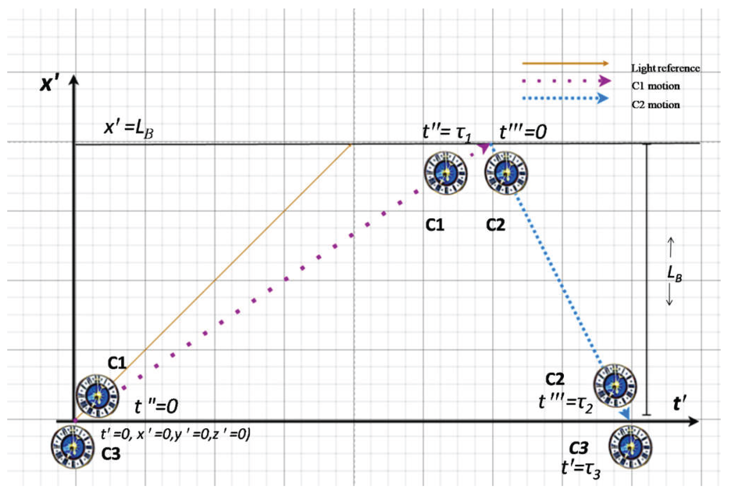
These findings suggest that the three-clock-based measurement result is a natural consequence of the spacetime geometry. This fact prompted an investigation into the possible implications of the three-clock scenario within Tangherlini spacetime, introduced in the 1958 doctoral thesis at Stanford University [3]. While the mathematical difference between the LT and the corresponding Tangherlini transformation (TT) matrices is subtle, the physical ramifications are vast. A similar scenario to that shown in Figure 1 can be applied by employing a hypothetical absolute rest frame concept and three moving clock frames in relative motion.
3. Methods
3.1. Background
Section 1 and Section 2 presented a validation of the distance formula in Equation (1)using the widely accepted Lorentz Transformation (LT) matrix for relativistic kinematics. While the validation of distance was expected, the emergence of Tangherlini’s velocity formulae in Equation (12) presented a distinct challenge. We recognised that the methodology must be adequate to the specific context in which Tangherlini’s Theory (TT) is perceived. TT remains outside the mainstream; indeed, rejection is often declared a priori. Will [4] (pp 325,326), referencing the Mansouri-Sexl [5] generalisation of coordinates transformation, remarked that adopting the infinite signal speed required for absolute clock synchronisation is a “perverse choice.” Such terminology can stifle objective scientific discussion. However, Tangherlini methodically derived the transformation from the Einstein field equations and he was fully aware of the instantaneous signal problem, expressing hope for absolute velocity detection via subluminal signals or rotational motion. Unlike earlier attempts—such as Eagle [6], requiring electrically controlled vibrating quartz rods, or Mansouri-Sexl [5], whose derivation appears to stem from a misinterpretation of LT time coordinates [5] (p 301 eq. 3.4 )—the method adopted here seeks to ground the discussion in objective, theoretical, and potentially measurable evidence.
3.2. The Adopted Approach
The following rules characterise our approach:
- We adopt the standard idealisations of Special Relativity (SR) [2], including the Einsteinian definition of inertial systems where Newtonian mechanics holds, and the use of ideal rigid rods within a Euclidean geometric framework.
- We assume that TT applied to vectors results in physically valid quantities unless a contradiction is proven, granting TT the same initial mathematical confidence as LT.
- Confidence in TT is further bolstered by the fact that, beyond Tangherlini’s General Relativity (GR) approach, these transformations can be derived from the fundamental postulates presented in Appendix A.
- To maintain a clear focus on the correspondence (or lack thereof) between these theories, we intentionally exclude Quantum Theory or complex GR metrics. Following the Rule of Analysis of Descartes in Discourse on Method [7] (p.35), we “divide each difficulty into as many parts as required” to achieve clarity.
- Following Rule 2, transformed physical quantities are deemed potentially measurable. The failure to determine absolute velocity excludes experimental confirmation otherwise theory must first be deemed theoretically sound and worthy of experimental effort. Similarly to LT approach we implicitly assume the idealisations and simplifications of the physical reality typical of the STR [2] such as adopting Einstein definition of inertial systems where Newtonian laws of mechanics hold [2] (p38) and foundation of coordinate systems grid is an ideal rigid rod standard and Euclidean Geometry [2] (p38)
3.3. Notation Convention
In the following sections we will be dealing with four coordinate systems: A representing the absolute reference frame (ARF), B for the base system and B1,B2 for clocks C1 and C2 respectively, which we recognise from the LT-based scenario. The notation used in this paper designates the last one or two symbols in relevant variable’s suffix to determine in which frame the quantity is observed/measured, while one or two preceding characters may define the frame to which the quantity belongs; hence, denotes the velocity of system B as measured in A. Similarly, for the C2 clock’s frame B2, we have , which is the velocity of system B2 in A. This allows clear distinction between similar quantities in different frames. Transformed vector symbols change suffix sequence accordingly however they often appear with one or more suierscripts
4. Three Clocks in Tangherlini Spacetime
The derivation of the transformations by Tangherlini provided an analytical relativistic framework similar to STR [2]. Originally named the “absolute Lorentz transformation” (ALT), the TT was derived from the Einstein field equation in the absence of gravitational sources. We found that the same transformation can be derived from first principles based on fundamental postulates, including the assumption of an absolute rest frame (ARF), as well as the experimentally established isotropy of the round-trip average speed of light and the controversial invariance of the instantaneous signal hypothesis (see Appendix A for the exact formulation of the postulates). No relativistic effects were assumed a priori; time dilation and length contraction emerged naturally.
Unlike the STR convention, where absolute velocity is outside the scope of measurement, we treat the ARF as a reference inertial system where is the absolute time variable; however, it is immeasurable. Thus far, according to the present consensus, absolute velocity suggestions appear fallacious, as once asserted by Eddington [8]. On the other hand, Tangherlini attempted to reason about the possibility of detecting absolute motion on the basis of the presented theory. First, he noted that if two distant clocks are not absolutely synchronised, it is not possible to calculate the one-way relative velocity of anything, because there is no way of correlating the time of arrival in terms of the time of departure [3] (p48). In Chapter 6 of [3] (p73–74), a claim is made that using subluminal signals, it would be possible to detect the absolute motion of the Earth. However, despite the focused, detailed analysis, no closed-form explicit solution or the exact details of the measurement method demonstrating this possibility are provided. Additionally, in the final chapter of [3] (p101), Tangherlini concluded that in the examples presented in the doctoral thesis, absolute velocity always cancels out when measurements are performed “in the usual manner”. We assume that these methods do not depend on the prior absolute synchronisation of separated clocks, which is impossible without instantaneous signals.
After determining that velocities can be measured with only three clocks, as shown in Equation (12), the question emerged whether this method was sufficiently ‘unusual’ to prove absolute velocity. The Unruh three-clock protocol [1] requires only three measurable proper times, and no two distant clocks appear to be synchronised other than by coincidence of their positions in a predefined location. We attempted the proof on the basis of a methodology similar to that in Section 2, but with the TT matrix, which is represented as follows:
The infinity subscript in the TT matrix symbol emphasises the role of the instantaneous signal postulate. Matrix (14) differs from the LT matrix (3) because of the absence of the space-dependent time coordinate, which is now zero. While the impossibility of absolute synchronisation with infinitely fast signals appears to be a fundamental obstacle, the significance of the TT framework would be profound if such obstacles could be circumvented.
4.1. Three-Clock Thought Experiment in Tangherlini 4D Spacetime
The graphical representation of the scenario differs slightly from that of the previous case in terms of the symbols of the axes, as shown in Figure 2.
This shows the perspective of the base system denoted by B with the system clock C3, which is an inertial moving system with respect to the hypothetical ARF denoted by A, which thus far, according to the present consensus, cannot be identified. However, it is treated here as a special purpose inertial system with time variable where no measurement can be made because no reference points are known in empty space.
In partial agreement with the objections of Poincaré [9] regarding the absolute space coordinate axes[2], we instead consider the absolute rest state to be a unique property of the subclass of inertial systems out of the class of all inertial systems rather than the state of the ‘void’. Our position disagrees with Newton’s concept of absolute space, which “remains always similar and immovable.” [10], but aligns with Einstein’s remark on the ether: “the idea of motion may not be applied to it” [11].
The inaccessibility of the featureless absolute space to measurement and the same with respect to any inertial absolute system A can be overcome by using the inverse transformation (TT−1) from any inertial system where times and lengths are measurable and can formally be related to A on the basis of the presented theory. At present, absolute velocity remains hypothetical until such time as its measurability is proved.
4.2. Derivation and Mathematical Reconciliation
In system B, we designate a fixed distant point as a 4-vector at which the worldline of C1 ends and that of C2 begins:
Instead of relative velocities as in the LT-based three-clock scenario, we look for absolute velocities with respect to the initially undefined absolute frame A. There is no obvious way to measure the relative velocity in Tangherlini spacetime; therefore, we need to introduce the base system’s absolute velocity vector inAwith an unknown magnitude . For simplicity, as in the STR standard configuration, it is aligned with the virtual x-axis of A and with the collinear x’-axis of B, as prescribed by the Tangherlini standard coordinate configuration (x- boost).
We can determine the vector equation of motion (EOM) of in A as by applying the inverse TT matrix (.
The variable in B needs to be eliminated from the transformed vector so that the absolute time is consistently expressed in absolute coordinates.
can now be expressed in absolute time coordinates as follows:
The moving clock C1 is associated with the symbol B1, which represents its local coordinate system, and must be converted to this system, in which is seen as a moving point towards the origin of B1. The absolute velocity of B1 in A is designated as . Therefore, it needs to be transformed using the transformation matrix .
The variable needs to be eliminated from the transformed vector so that it is consistently expressed in coordinates.
After the substitution, can be expressed in B1 terms of the coordinate as follows:
The marker in the B1 frame, appears to move towards the B1 origin. The time at which clock C1 coincides with the marker is when its coordinate is 0:
The trip duration of clock C1 is now determined. Because of the downwards worldline orientation, the duration of clock C2 follows the same formula (22), but with a different velocity symbol and with the sign inverted so that remains positive.
We have determined the durations on paths from the perspective of moving clocks C1 and C2; now, we need to find the relative velocities and of these clocks in B and the time of the round trip measured by clock C3. The vector EOM of C1 in A is given by the 4-vector :
Applying TT to yields the following:
After (25) is converted to the local time t’, the relative EOM of C1 is as follows:
Similarly, for B2:
The relative velocities and are then the same formulae except for replacing :
The round-trip time registered by clock C3 is as follows:
We obtain the system of the following three nonlinear equations from Equations (22), (23) and (29).
From this system, we cannot calculate because we have three unknown velocities and therefore four unknowns with only three equations. We cannot rely on the currently not practically feasible method described in Section 2. This is, however, not an obstacle because is a free parameter that can be measured by traditional methods, particularly by using the return time of the light signal on the round trip:.
The system solution was attempted using Maple™ 2019. Unfortunately, despite the unusual nature of the three-clock method, which does not explicitly rely on distant clock synchronisation, no solution was found due to usual cancellation.
While confirming and analysing the disappointing but widely expected null result, an important connection was found between the Minkowski and Tangherlini frameworks.
- 1.
- Using proper times represented by Equations (30);
- 2.
- Substituting them into the positive root of the equation for LB and to all velocity roots from Equations (12); and
- 3.
- Assuming that and is a real positive number, the result of algebraic simplification is as follows:
This was as expected for . The absolute velocities did cancel out; thus, remained invariant. However, no cancellation can be seen for the STR relative velocities. One instance of the STR velocity can be the result of an unlimited number of combinations of . Measuring is insufficient to solve for an absolute velocity because of one extra degree of freedom. At this point, all the classic predictions seem to confirm the postulate of relativity as formulated by Poincaré [12] (drafted in June 5, 1905), placing the inability to detect the absolute movement of the Earth as the foundation (refer to the discussion on page). Poincaré reported that his principle, which is consistent with the Lorentz transformation, was thoroughly reviewed and rederived with full mathematical rigour [12]. This finding made it pointless for him and most of his successors to look elsewhere. However, the peculiar relationships in Equation (31) and their potential significance triggered further investigations.
4.3. Variable Speed of Light vs. Conventional Isotropy
The variable light pulse velocities in the standard coordinate configuration in the Tangherlini framework are given as follows:
where and are the positive variable magnitudes of the velocity of light on the -axis in the positive and negative directions, respectively; hence, all relative velocities are functions of absolute velocities. First, we analyse the results in Equation (13). Using proper times given in Equation (30) and substituting them into the first equation of Equation (13), we obtain the following:
where is the current time coordinate in the propagation of C1 in B in the LT-based scenario in Figure 1 and is the coinciding position of C1.
At the same physical location in the STR and Tangherlini frameworks, . Using the first equation of Equation (28), we obtain the following:
Using Equations (33) and (34), we can solve the following system for and :
The solution of interest is with , while the other solution for has no useful value:
This allows bidirectional conversions to/from the Tangherlini and STR frameworks because the -axes are identical when they statically coincide in B. This also shows that the irreducible degree of freedom with being eliminated from the scope is the main reason behind all cancellations. It now appears that removing this freedom could occur only by implementing the nonexistent instantaneous signal synchronisation. Fortunately, this is not the case.
4.4. Closing the Gap
Our attention shifted towards identifying a missing equation that would allow for the recovery of the absolute velocity . Thus far, our derivation of the TT has assumed an empty, featureless, and passive space, focusing on the relative kinematics between a hypothetical privileged inertial system and any other inertial frame. The relativistic TT relation was derived from the empirical isotropy of the average round-trip speed of light, without assuming a specific physical cause for this behaviour. However, it is logical to conclude that this behaviour is not caused by the inertial systems themselves. This raised a critical question: is there an overlooked property of light that could resolve the absolute velocity? The most vital observation is that while light is emitted and absorbed by atoms to facilitate measurement, its orderly, causal propagation from point to point is a property of the vacuum and the electromagnetic field itself. Once emitted, a beam of light may exist independently of any inertial system, propagating as a coherent entity—much like a “rigid rod” of fixed length. Considering light from a distant star that may no longer exist, it travels through the void and interacts with any inertial system it encounters. At the moment of interaction, the original source is irrelevant; only the freely propagating beam matters. While a stationary observer in the ARF would measure an intrinsic frequency, a moving observer in system B would measure a Doppler-shifted frequency. This invites us to look beyond the average round-trip speed of light and examine the Doppler effect as an additional fundamental property. We consider a monochromatic electromagnetic wave propagating along the -axis from the positive side towards a detector and clock C3 at the origin of the base system B.
Let K be the wave 4-vector of the incoming wave in free space or rather in the ARF:
To convert this vector to B, we apply TT as follows:
where .
The explicit presence of in Equation (38) determines the absolute velocity, assuming that the angular frequency and the wave number can be accurately measured. The latter may be much more difficult to accomplish than the former. By shifting focus from the clocks to the light beam in transit, the missing equations are now identified. Unlike clocks, a freely propagating electromagnetic wave train has an intrinsic spatial and temporal periodicity that is governed by the vacuum itself, not the observer’s synchronisation convention. By measuring the local frequency and the local wavenumber (e.g., via the movable intensity sensor protocol), we can possibly determine two unknowns: the absolute velocity and the original , which can be obtained by solving the following system of equations:
The solution of the above system is:
This is quite interesting result. We once declared that there are no features in empty space, so we cannot find any reference point—anything to measure—except for light that never stops. Firstly, we can find not only the absolute velocity in an unknown ARF but also the so far unknown light angular frequency, where no clock and no coordinate system exist. The hypothetical ARF becomes potentially measurable. This would be an ultimate connection with absolute rest state which CMB might represent.
The above seems to be the most direct way of finding . Better still, is to exploit the property of the ratio.
This equation is of ultimate simplicity but relies on the same direct measurement of . Note that if the ratio R = -1, as in the STR framework, =0. While this principle of measurement of absolute velocity appears to be valid, it is only a raw proof of concept requiring the physics community to generalise it to a 3D context such that the velocity vector can be fully identified and engineers to make the method practical and sensitive. The hope is that measurements of velocities with respect to the Cosmic Microwave Background (CMB) provide sufficient grounds to expect that adequate measurement method can be found in due time. By identifying the absolute velocity in Equation (41), we provide a potentially fundamental theoretical basis for CMB velocity measurements without contradicting STR, which remains valid for the vast majority of physical contexts where absolute motion does not alter local outcomes, consistent with the cancellations resulting from Equations (30). This finding may potentially closes the over-120-year gap in understanding the fundamental nature of flat spacetime, unaffected by strong gravitational fields.
There is however, one major problem that must be explained. The frequency does not agree with overwhelming consensus. For example, in the publication of Drągowski, M., Włodarczyk [13] the authors demonstrated that Doppler effect under absolute transformation is indistinguishable from that derived from the Lorentz. We have expanded this research in order to reconcile the discrepancy and preliminary results look intriguing.There is, however, one major problem that must be explained. The frequency component derived here does not agree with the overwhelming consensus. For example, Drągowski and Włodarczyk [13] demonstrated that the Doppler effect under absolute transformation should be indistinguishable from that derived from the Lorentz transformation. We have expanded upon this research to address the observed discrepancy; preliminary results are intriguing and suggest a path toward reconciling these two frameworks.
5. Discussion and Conclusions
Given the unresolved discrepancy in the Doppler shift results, which persists despite verified algebraic consistency, the Discussion and Conclusions sections are deferred pending final resolution of the underlying model. Ongoing work is addressing this problem, suggesting even deeper connection between the Tangherlini and Lorentz frameworks that promises their ultimate reconciliation.
5.1. Conclusions
To be continued.
| [1] | Bill Unruh, undisclosed private communication, according to [1]. |
| [2] | This idea came from Poincaré claiming that “absolute space is nonsense, and it is necessary for us to begin by referring space to a system of axes invariably bound to our body (which we must always suppose put back |
Author Contributions
The author contributed to all aspects of the work.
Funding
This research received no funding.
Institutional Review Board Statement
Not applicable.
Informed Consent Statement
Not applicable.
Data Availability Statement
New data were generated from the mathematical model. Detailed Maple computation results may be available upon request.
Conflicts of Interest
The author declares no conflicts of interest.
Abbreviations
The following abbreviations are used in this manuscript:
| ALT | Absolute Lorentz Transformation |
| AR | Absolute Rest |
| ARF | Absolute Rest Frame |
| CMB | Cosmic Microwave Background |
| EOM | Equation of Motion |
| GR | General Relativity |
| LT | Lorentz Transformation |
| STR | Special Theory of Relativity |
| TT | Tangherlini Transformation |
Appendix A. On Absolute Rest, AVelocity and Tangherlini Transformation
Tangherlini’s derivation of the transformation applied in this paper was originally based on the Einstein field equation of general relativity (GR), resulting in transformation equations compatible in structure with the LT equations derived by Einstein, as presented in [2] (p48). The arrangement of the two relatively moving coordinate systems can be referred to as the standard configuration, where the relative velocity vector is aligned with the first spatial axis (usually x). The mathematical representations of the TT, the postulates leading to its derivation and resulting properties may be collectively referred to as the TT framework.
With respect to the TT framework, the absolute rest frame must be postulated a priori to allow derivation when using a method other than Tangherlini’s approach based on GR. For example, in Section 3, Selleri [14] defines the absolute frame as the one where the velocity of light is the same in any direction while not demanding moving frames to follow the same rule. The impossibility of absolute synchronisation with instantaneous signals—let alone without them—appears to be the fundamental obstacle to the practical use of TT on a larger scale. The TT framework seems to be the only sensible but impractical alternative to the STR framework. Both frameworks share the same foundation, which is the empirical law of isotropy of the round-trip average speed of light discovered by Michelson and Morley [15].
The TT framework can be derived from first principles of Newtonian kinematics without reference to noninertial rotational motion or forcing postulates of length contraction or time dilation, as was the case in some previous approaches. However, the frequently analysed Sagnac effect seems to be a legitimate approach.
The necessary and sufficient set of postulates/conditions for completely defining the TT are as follows:
Postulate 1:
There exists an absolute rest frame (ARF) represented by an inertial system A, withthree Cartesian coordinate axes that can be bound (aligned) to preexisting axes of an inertial system M at time t=0 and t’=0. In that system, the one-way velocity of light is constant and equal to c in all directions, and there is only one system A (together with all its possible translations and rotations, all being at rest with it).
Postulate 2:
The round-trip average speed of light in any inertial system is a constant, whose value c= 299792458 m/s, and is independent of the relative direction and velocity of those systems.
Postulate 3:
An instantaneous signal being represented as the limit of all signals moving in the same direction with ever increasing velocity, observed in the absolute inertial system A as,is invariant in all inertial frames such that when observed in an inertial moving system M of the absolute velocity vMA, it is, where.
Constraint 1:
The spatial origin of systemMmoving in the system A coordinates transforms to the origin point in M at rest with itself as M(0,0,0) at every instance of time t’.
Constraint 2:
The determinant of the linearcoordinate transformation matrixis equal to +1,as in the case of the LT and Galilean transformation matrices.
The TT matrix meeting the postulates and constraints can be derived and is shown in Equation (14). Including the full derivation process in this paper would exceed a sensible publication word count limit.
References
- Matsas George, E. A. The number of fundamental constants from a spacetime-based perspective. Scientific Reports 2024, 14, 22594. [Google Scholar] [CrossRef] [PubMed]
- Einstein, A. “On the Electrodynamics of Moving Bodies,” in The Principle of Relativity; Dover Publications, Inc.: USA, 1923; p. 140. Available online: https://archive.org/details/principleofrelat0000halo/page/n3/mode/2up.
- Tangherlini, F.R. The Velocity of Light in Uniformly Moving Frame- PhD Disertation Stanford University1958. The Abraham Zelmanov Journal 2009, vol. 2, 44–110. [Google Scholar]
- Will M. C., Theory and Experiment in Gravitational Physics; Cambridge University Press: Cambridge, 1993.
- Mannnsouri, R.; Sexl, R.U. A Test Theory of Special Relativity: I. Simultaneity and Clock Synchronization. General Relativity and Gravitation 1977, vol. 8(no. 7), 497–513. [Google Scholar] [CrossRef]
- Eagle, A. A criticism of the special theory of relativity. Lond. Edinb. Dubl. Phil. Mag. & J. Sci. vol. 26, 410–414, 1938. [CrossRef]
- Descartes, R. Discourse On The Methodof Conducting One’s Reason Well and of Seeking the Truth in the Sciences; Press of Jan Maire: Leiden, 1637; Available online: https://dn710004.ca.archive.org/0/items/descartes-discourse-on-method-heffernan-archive/.
- Eddington, A.S. The Nature of the Physical World; Cambridge University Press: Cambridge, 1929; Available online: https://www.gutenberg.org/cache/epub/72963/pg72963-images.html.
- Poincaré, H. The Value of Science; Science Press: New York, 1907. [Google Scholar]
- Newton, I. The Mathematic Principles of Natural Philosophy; Daniel Adee: New York, 1848. [Google Scholar]
- Einstein, A. “Ether and the Theory of Relativity,” in Sidelights on Relativity; METHUEN & CO. LTD.: London, 1922; Volume ch. 1, p. 24. [Google Scholar]
- Poincaré, H. Sur la dynamique de l’électron. Rendiconti del Circolo Matematico di Palermo 1906, 21 vol. 21, 1906, 129–176. pp. 129–176. [Google Scholar] [CrossRef]
- Drągowski, M.; Włodarczyk, M. The Doppler Effect and the Anisotropy of the Speed of Light. Found Phys. 2020, vol. 50, 429–440. [Google Scholar] [CrossRef]
- Selleri, F. “Noninvariant One-Way Speed Of Light And LocallynEquivalent Reference Frames,” Found. Phys. Lett. 1997, vol. 10, 73–8. [Google Scholar] [CrossRef]
- Michelson, A. A.; Morley, E. W. On the relative motion of the earth and the luminiferous ether. Am. J. Sci. vol. 34(no. 203), 333–345, 1887. [CrossRef]
- Einstein, A. ““Discussion” Following Lecture Version of “Theory of Relativity”,” in The Collected Papers of Albert Einstein. In The Swiss Years Writings 1909-1911 (English translation supplement); Princeton University Press: Princeton, 1994; Volume 3, p. 353. [Google Scholar]
Figure 1.
The three-clock scenario (angles not to scale).
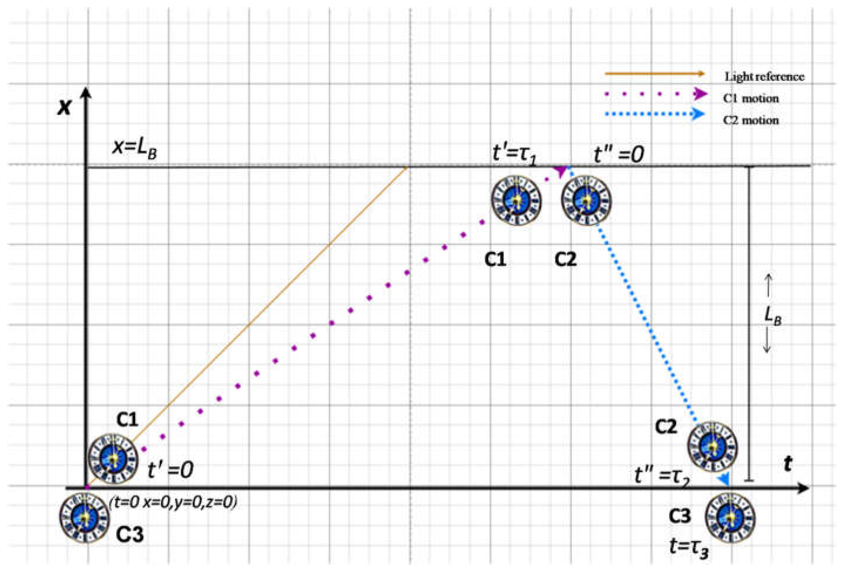
Figure 2.
Two-clock round-trip scenario in system B (angles not to scale).
Disclaimer/Publisher’s Note: The statements, opinions and data contained in all publications are solely those of the individual author(s) and contributor(s) and not of MDPI and/or the editor(s). MDPI and/or the editor(s) disclaim responsibility for any injury to people or property resulting from any ideas, methods, instructions or products referred to in the content. |
© 2026 by the authors. Licensee MDPI, Basel, Switzerland. This article is an open access article distributed under the terms and conditions of the Creative Commons Attribution (CC BY) license (http://creativecommons.org/licenses/by/4.0/).
Copyright: This open access article is published under a Creative Commons CC BY 4.0 license, which permit the free download, distribution, and reuse, provided that the author and preprint are cited in any reuse.


