Measuring Velocity Using Moving Clocks—The Surprising Test of Tangherlini’s Theory

1. Introduction

In the 2024 publication [1] Matsas et. al, presented an intriguing concept of time being the only base unit needed to construct derived units of measure for all physical quantities currently defined within LMT dimensions. The most striking is distance measurement using only three inertial systems clocks: one stationary C3 and two relatively moving C1 and C2 in a round trip arrangement as shown in Figure 1. Such stunning result cannot be achieved in Galilean systems but in Minkowski spacetime it can, because it has on degree of freedom less than the Galilean due to the Einstein’s velocity of light postulate. The distance-measuring formula published in [1] is originally based on three inertial clocks world lines on Minkowski diagrams in a triangular arrangement. The distance formula is:

$$D={\displaystyle \frac{\sqrt{\left[{\left({{\mathsf{\tau }}_3}^2-{{\mathsf{\tau }}_1}^2-{{\mathsf{\tau }}_2}^2\right)}^2-4{{\mathsf{\tau }}_1}^2{{\mathsf{\tau }}_2}^2\right]}}{2{\mathsf{\tau }}_3}},$$

(1)

where ${\mathsf{\tau }}_3$ is the C3 clock time at the stationary system origin and ${\mathsf{\tau }}_{1,}{\mathsf{\tau }}_2$are the moving clocks’ C1 and C2 respective trips durations at unspecified velocities. This formula can be expanded to the following equivalent expression:

$$D={\displaystyle \frac{\sqrt{{{\mathsf{\tau }}_1}^4-2{{\mathsf{\tau }}_1}^2{{\mathsf{\tau }}_2}^2-2{{\mathsf{\tau }}_1}^2{{\mathsf{\tau }}_3}^2+{{\mathsf{\tau }}_2}^4-2{{\mathsf{\tau }}_2}^2{{\mathsf{\tau }}_3}^2+{{\mathsf{\tau }}_3}^4}}{2{\mathsf{\tau }}_3}}$$

(2)

Clock C1 moves from the origin in the positive direction of x and the other from x=L_B in the opposite direction towards the origin. The motion protocol slightly differs from the original in [1] but it is equivalent and illustrated in Figure 1.

• The stationary system is named ‘System B’ as the Base platform lab for the thought experiment.
• Clock C1arrives from the negative part of the x-axis at constant yet unknown velocity v₁ and resets itself to tꞌ=0.
• The stationary clock C3 also resets itself to 0 at the C1 departure event.
• Clock C2 is launched with velocity v₂ from far positive side on the x-axis, on a collision course with C1 with a negligible y offset in order to continue its motion towards the origin after the close encounter with C1 during which C2 is reset to tꞌꞌ= 0.
• This round trip arrangement is maintained for compatibility with the Minkowski space triangular arrangement in the original [1] helping geometric reasoning. However, in practice, each trip can be executed sequentially because durations are independent of specific times the motions start.
• Upon the encounter with C2, C1 broadcasts the time tꞌ=${\tau }_1$ to the Base origin for future reckoning.
• Clock C2 arrives to the C3 origin and communicates the time tꞌꞌ =${\tau }_2$ to the Base for future reckoning.
• The stationary C3 clock Base, records the local time of arrival of C2 as t=${\tau }_3$ which is the duration of the round trip between x=0 and x= L_B (which is unknown) then back to x=0.
• We have sufficient data to determine not only the unknown L_B. but also equally unknown velocities v₁ and v₂.

2. Distance and Velocities Calculation in Minkowski Spacetime

All considerations in the next sections implicitly admit idealisations and simplifications of physical reality typical to the framework of the STR [2].

The preferred method for derivations is linear algebra with Lorentz Transformation matrix defined as:

$$\begin{gathered} {\Lambda }_v=\left[\begin{array}{cccc}{\gamma }_v& -v{\displaystyle \frac{{\gamma }_v}{c}}& 0& 0\\ -v{\displaystyle \frac{{\gamma }_v}{c}}& {\gamma }_v& 0& 0\\ 0& 0& 1& 0\\ 0& 0& 0& 1\end{array}\right] \\ { \gamma }_v=1/\sqrt{1-v^2/c^2}, \end{gathered}$$

(3)

Assuming we have the Base stationary inertial system B represented by a 4D Cartesian coordinates system, where we analyze the motion of two inertial point masses PM₁ and PM₂ represented by clocks C1 and C2 moving along the x-axis. The four-vector XL_B represents an unknown, emergent reference distance as follows:

$$X{L}_B=\left[\begin{array}{c}\begin{array}{c}ct\\ L_B\\ 0\end{array}\\ 0\end{array}\right].$$

(4)

The transformation of the fixed $X{L}_B$ inBto the local C1 coordinates using Lorentz transformation matrix ${\Lambda }_{v1}$multiplied by $X_{LB}$ yields the moving point $X_{L1}$ approaching the C1 origin:

$${\Lambda }_{v1}\left[\begin{array}{c}\begin{array}{c}ct\\ L_B\\ 0\end{array}\\ 0\end{array}\right]=\left[\begin{array}{c}\begin{array}{c}{\displaystyle \frac{c^{2}t-L_B{v}_1}{\sqrt{c^2-{v_1}^2}}}\\ {\displaystyle \frac{L_B-v_{1}t}{\sqrt{c^2-{v_1}^2}}}\\ 0\end{array}\\ 0\end{array}\right]\equiv X_{L1}.$$

(5)

The transformed vector $X_{L1}$is in terms of the B’s system time t and needs to be converted to local time t' of C1.

$$X{L}_1\left[1\right]/c=t\text{'}\Rightarrow t={\displaystyle \frac{\sqrt{c^2-{v_1}^2}ct+L_B{v}_1}{c^2}}.$$

(6)

The converted vector in the local primed coordinates is obtained by the substitution of the t expression from equation (6) and subsequent simplifications:

$$X_{L1=}^{\text{'}}\left[\begin{array}{c}\begin{array}{c}ct\text{'}\\ {\displaystyle \frac{{{-c\sqrt{c^2-{v_1}^2{v}_{1}t\text{'}}+L}_{B}c}^2-L_B{v_1}^2}{c\sqrt{c^2-{v_1}^2}}}\\ 0\end{array}\\ 0\end{array}\right].$$

(7)

The time it takes for the $L_B$ to come in contact with C1 origin can be found when $X_{L1}^{\text{'}}\left[1\right]=0$, calculated from the following equation:

$${{-c\sqrt{c^2-{v_1}^2{v}_{1}t\text{'}}+L}_{B}c}^2-L_B{v_1}^2=0\Rightarrow t^{\text{'}}={\displaystyle \frac{L_B\sqrt{c^2-{v_1}^2}}{v_{1}c}}\equiv {\tau }_1.$$

(8)

C2 differs from C1 only by the magnitude of the velocity hence by analogy:

$${{-c\sqrt{c^2-{v_2}^2{v}_{2}t\text{'}}+L}_{B}c}^2-L_B{v_2}^2=0\Rightarrow t^{\text{'}}={\displaystyle \frac{L_B\sqrt{c^2-{v_2}^2}}{v_{2}c}}\equiv {\tau }_2.$$

(9)

In the Clock C3, the duration of the round trip is the sum of successive durations on each segment given by the elementary expression:

$${\tau }_3\equiv {\displaystyle \frac{L_B}{v_1}}+{\displaystyle \frac{L_B}{v_2}}.$$

(10)

Given the clock times were measured, we have three equations and three unknowns:${L_B, v}_1$and $v_2$:

$$\left\{\begin{array}{c}{\tau }_1={\displaystyle \frac{L_B\sqrt{c^2-{v_1}^2}}{v_{1}c}}\\ {\tau }_2={\displaystyle \frac{L_B\sqrt{c^2-{v_2}^2}}{v_{2}c}}\\ {\tau }_3={\displaystyle \frac{L_B}{v_1}}+{\displaystyle \frac{L_B}{v_2}}. \end{array}\right.$$

(11)

The solution of the non-linear system of equations (11) with respect to $L_B$,$v_1$,$v_2$ is:

$$\left\{\begin{array}{c}{L}_B={\displaystyle \frac{\pm \mathrm{c}\sqrt{{{\mathsf{\tau }}_1}^4-2{{\mathsf{\tau }}_1}^2{{\mathsf{\tau }}_2}^2-2{{\mathsf{\tau }}_1}^2{{\mathsf{\tau }}_3}^2+{{\mathsf{\tau }}_2}^4-2{{\mathsf{\tau }}_2}^2{{\mathsf{\tau }}_3}^2+{{\mathsf{\tau }}_3}^4}}{2{\mathsf{\tau }}_3}}\\ v_1={\displaystyle \frac{\pm \mathrm{c}\sqrt{{{\mathsf{\tau }}_1}^4-2{{\mathsf{\tau }}_1}^2{{\mathsf{\tau }}_2}^2-2{{\mathsf{\tau }}_1}^2{{\mathsf{\tau }}_3}^2+{{\mathsf{\tau }}_2}^4-2{{\mathsf{\tau }}_2}^2{{\mathsf{\tau }}_3}^2+{{\mathsf{\tau }}_3}^4}}{{{\mathsf{\tau }}_1}^2-{{\mathsf{\tau }}_2}^2+{{\mathsf{\tau }}_3}^2}}\\ v_2={\displaystyle \frac{\pm \mathrm{c}\sqrt{{{\mathsf{\tau }}_1}^4-2{{\mathsf{\tau }}_1}^2{{\mathsf{\tau }}_2}^2-2{{\mathsf{\tau }}_1}^2{{\mathsf{\tau }}_3}^2+{{\mathsf{\tau }}_2}^4-2{{\mathsf{\tau }}_2}^2{{\mathsf{\tau }}_3}^2+{{\mathsf{\tau }}_3}^4}\mathrm{c}}{{{\mathsf{\tau }}_1}^2-{{\mathsf{\tau }}_2}^2-{{\mathsf{\tau }}_3}^2}}.v \end{array}\right.$$

(12)

The $L_B$ expression is only valid for the positive value. Although it appears different from the original equation (1), it matches the expanded equivalent form in equation (2). Naturally, we have the speed of light constant c absent in (2), which was suppressed to non dimensional one in [1], because of Minkowski diagrams convention.

The ability to measure $L_B$ using clocks only, was a very interesting discovery, but the ability to measure velocity without synchronised clock is even more interesting. On the surface, a constant velocity measurement requires two distant synchronised clocks (except for Doppler radars and two successive light round trip measurements). The surprising element of velocity formulae from equations (12) is that no distance is explicitly needed, because it was all factored in time constants’ arrangement in (12). Three independent moving clocks relative to each other indicate their proper time without regards to any coordinate systems (if we forget that STR was needed to derive the equations (12) ), but clocks have no knowledge of other clocks or coordinates systems. It is all arranged in space this way by nature. This fact prompted an investigation on consequences of the three clocks scenario in Tangherlini spacetime that was introduced in his doctoral thesis in 1958 [2] at Stanford University. There is a subtle difference between the Lorentz Transformation (LT) and Tangherlini Transformation (TT) matrices, but physical ramifications are vast. Similar scenario to that shown in Figure 1 can be applied, while using a hypothetical absolute rest frame, plus three moving frames in relative motion. This can be examined in an attempt to replicate similar derivation as in this section with necessary modifications.

3. Three Clocks in Tangherlini Spacetime

Tangherlini derived what we now call Tangherlini Transformation resulting in a simplified framework, similar to that in the STR [3]. It was originally named as “The Absolute Lorentz Transformation” (ALT) and derived from Einstein Field Equation in the absence of gravitational sources. We found no need to use General Relativity GR) for this purpose and derived it from first principles in a similar way the STR was derived with necessary changes in fundamental postulates. The fundamental postulates and constraints applied in the derivation process (not presented here) are described in the Appendix A. The TT can be represented in the matrix form as follows:

$$\begin{gathered} {\mathsf{\Omega }}_{\infty }^v=\left[\begin{array}{cccc}1/{\gamma }_v& 0& 0& 0\\ -v{\displaystyle \frac{{\gamma }_v}{c}}& {\gamma }_v& 0& 0\\ 0& 0& 1& 0\\ 0& 0& 0& 1\end{array}\right] \\ \mathrm{where} {\gamma }_v=1/\sqrt{1-v/c^2}. \end{gathered}$$

(13)

The infinity symbol in ${\mathsf{\Omega }}_{\infty }^v$emphasises the underlying role of the instantaneous signal and v - the generic velocity. The TT matrix (13) differs from the LT matrix (3) by the absence of the second element in the first row which is now zero while the factor γ_v is inverted. The disappearance of the space dependent time coordinate is solely due to the new Postulate of invariance of the instantaneous signal (See Appendix A). The impossibility of the absolute synchronization with infinitely fast signals appears as the fundamental obstacle for using TT in any practical application, yet the significance of the TT framework cannot be overstated.

3.1. Three Clocks Experiment in the Tangherlini 4D Spacetime

The graphical representation of the scenario slightly differs from the previous case by symbols of axes as shown in shown in Figure 2. It shows the perspective of the Base system denoted as B with the system clock C3 which is an inertial moving system with respect to the hypothetical Absolute Rest (AR) system A, which so far, according to the current consensus, cannot be identified. However, it is treated here as a special purpose reference inertial system with a system clock C0 with time variable t where no measurement can be made because its reference point is unknown.

In the system B we designate a fixed distant point X_LB as a four-vector:

$$X{L}_B=\left[\begin{array}{c}\begin{array}{c}ct\text{'}\\ L_B\\ 0\end{array}\\ 0\end{array}\right].$$

(14)

Instead of relative velocities in the LT based three clocks scenario, we use absolute velocities with respect to A. There is no simple way to find relative velocity in Tangherlini spacetime, therefore we need to introduce the Base System Absolute Velocity vector $\overrightarrow{{\mathit{v}}_{\mathit{B}\mathit{A}}}$ of the unknown magnitude v_BA which for simplicity like in the STR convention, it is aligned with the x-axis of A and xꞌ- axis in B (x-boost configuration).

The convention in this paper designates the last letter in the suffix to determine in which frame the quantity is observed/measured, while one or two preceding characters define to which frame the quantity belongs, hence v_BA reads: ‘the velocity of the system B as measured in A. We can determine the vector equation of motion (EOM) of X_LB in A, applying the inverse Tangherllini Transformation.

$$Inv\left({\mathsf{\Omega }}_{\infty }^{v_{BA}}\right)\left[\begin{array}{c}\begin{array}{c}c{t}^{\text{'}}\\ L_B\\ 0\end{array}\\ 0\end{array}\right]=\left[\begin{array}{c}\begin{array}{c}{\displaystyle \frac{c^2{t}^{\text{'}}}{\sqrt{c^2-{v_{BA}}^2}}}\\ {\displaystyle \frac{\left(v_{BA}{t}^{\text{'}}+L_B\right){c^2-L}_B{v_{BA}}^2}{c\sqrt{c^2-{v_{BA}}^2}}}\\ 0\end{array}\\ 0\end{array}\right]\equiv X_{LBA},$$

(15)

$${\displaystyle \frac{X_{LBA}\left[1\right]}{c}}=t\Rightarrow t^{\text{'}}={\displaystyle \frac{t\sqrt{c^2-{v_{BA}}^2}}{c}}.$$

(16)

$X_{LBA}$ can be expressed in the absolute time coordinate t as:

$$X_{LBA}=\left[\begin{array}{c}\begin{array}{c}ct\\ {\displaystyle \frac{c\sqrt{c^2-{v_{BA}}^2}{v_{BA}t{+L}_B{c}^2-L}_B{v_{BA}}^2}{c\sqrt{c^2-{v_{BA}}^2}}}\\ 0\end{array}\\ 0\end{array}\right].$$

(17)

The moving clock C1 was assigned the symbol B1 to represent its local coordinate system and $X_{LBA}$ must be converted to this system, in which L_B is seen as moving point towards the origin of B1. The absolute velocity of B1 in A is designated as v_B1A. So it needs to be transformed using the transformation matrix ${\mathsf{\Omega }}_{\infty }^{v_{B1A}}$.

$${{\mathsf{\Omega }}_{\infty }^{v_{B1A}}X}_{LBA}=X_{LB1A}=\left[\begin{array}{c}\begin{array}{c}\sqrt{c^2-{v_{B1A}}^2}t\\ {\displaystyle \frac{ct(v_{BA}-v_{B1A})\sqrt{c^2-{v_{BA}}^2}{{+L}_B{c}^2-L}_B{v_{BA}}^2}{\sqrt{c^2-{v_{BA}}^2}\sqrt{c^2-{v_{B1A}}^2}}}\\ 0\end{array}\\ 0\end{array}\right],$$

(18)

$${\displaystyle \frac{X_{LB1A}\left[1\right]}{c}}=t^{\text{'}\text{'}}\Rightarrow t^{\text{'}\text{'}}={\displaystyle \frac{ct}{\sqrt{c^2-{v_{B1A}}^2}}}.$$

(19)

$X_{LB1A}$ can be expressed in B1 time coordinate tꞌꞌ as:

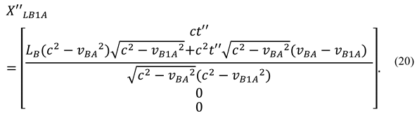
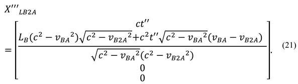
The same transformation must be performed for analogous C1 clock system designated as B2 so the same expression applies with the exception of v_B1A becoming v_B2A, hence:

The time the clock C1 coincides with $L_B$ is when it touches the origin of B1, so is then:

$${X\text{'}\text{'}}_{LB1A}\left[2\right]=0\Rightarrow t^{\text{'}\text{'}}={\displaystyle \frac{L_B\sqrt{c^2-{v_{BA}}^2}\sqrt{c^2-{v_{B1A}}^2}}{c^2({-v}_{BA}+v_{B1A})}}\equiv {\tau }_1,$$

(22)

and for B2:

$${X\text{'}\text{'}\text{'}}_{LB2A}\left[2\right]=0\Rightarrow t^{\text{'}\text{'}\text{'}}={\displaystyle \frac{L_B\sqrt{c^2-{v_{BA}}^2}\sqrt{c^2-{v_{B2A}}^2}}{c^2({-v}_{BA}+v_{B2A})}}\equiv {\tau }_2.$$

(23)

We have determined durations of flight from the perspective of moving clocks C1 and C2, now we need to find the relative velocities v₁ and v₂ of clocks in B and the time of the round trip ${\tau }_3$ measured by the clock C3. The vector EOM of C1 in A is given by the four-vector X_B1A:

$$X_{B1A}=\left[\begin{array}{c}\begin{array}{c}ct\\ v_{B1A}t\\ 0\end{array}\\ 0\end{array}\right].$$

(24)

Applying TT to $X_{B1A}$ yields:

$${\mathsf{\Omega }}_{\infty }^{v_{BA}}{X}_{B1A}=X_{B1B}=\left[\begin{array}{c}\begin{array}{c}\sqrt{c^2-{v_{BA}}^2}t\\ {\displaystyle \frac{ct\left({-v}_{BA}{+v}_{B1A}\right)}{\sqrt{(c^2-{v_{BA}}^2)}}}\\ 0\end{array}\\ 0\end{array}\right].$$

(25)

After converting (25) to the local time tꞌ:

$${X\text{'}}_{B1B}=\left[\begin{array}{c}\begin{array}{c}c\text{'}t\\ {\displaystyle \frac{c^{2}t\text{'}\left({-v}_{BA}{+v}_{B1A}\right)}{(c^2-{v_{BA}}^2)}}\\ 0\end{array}\\ 0\end{array}\right].$$

(26)

Similarly for B2:

$${X\text{'}}_{B2B}=\left[\begin{array}{c}\begin{array}{c}c\text{'}t\\ {\displaystyle \frac{c^{2}t\text{'}\left({-v}_{BA}{+v}_{B2A}\right)}{(c^2-{v_{BA}}^2)}}\\ 0\end{array}\\ 0\end{array}\right].$$

(27)

Velocities v1 and v2 are then:

$$v_1={\displaystyle \frac{c^2\left({-v}_{BA}{+v}_{B1A}\right)}{\left(c^2-{v_{BA}}^2\right)}}\mathrm{br}-\mathrm{to}-\mathrm{break} v_2={\displaystyle \frac{c^2\left({-v}_{BA}{+v}_{B2A}\right)}{\left(c^2-{v_{BA}}^2\right)}},$$

(28)

The round tip time registered by clock C3 is:

$${\tau }_3={\displaystyle \frac{L_B}{v_1}}+{\displaystyle \frac{L_B}{v_2}}={\displaystyle \frac{L_B\left(c^2-{v_{BA}}^2\right)}{c^2\left({-v}_{BA}{+v}_{B1A}\right)}}+{\displaystyle \frac{L_B\left(c^2-{v_{BA}}^2\right)}{c^2\left({-v}_{BA}{+v}_{B2A}\right)}}.$$

(29)

We obtain the system of 3 non linear equations from (22)(23)(28)(29):

$$\left\{\begin{array}{c}{\tau }_1={\displaystyle \frac{L_B\sqrt{c^2-{v_{BA}}^2}\sqrt{c^2-{v_{B1A}}^2}}{c^2({-v}_{BA}+v_{B1A})}} \\ {\tau }_2={\displaystyle \frac{L_B\sqrt{c^2-{v_{BA}}^2}\sqrt{c^2-{v_{B2A}}^2}}{c^2({-v}_{BA}+v_{B2A})}} \\ {\tau }_3={\displaystyle \frac{L_B\left(c^2-{v_{BA}}^2\right)}{c^2\left({-v}_{BA}{+v}_{B1A}\right)}}+{\displaystyle \frac{L_B\left(c^2-{v_{BA}}^2\right)}{c^2\left({-v}_{BA}{+v}_{B2A}\right)}}\end{array}\right.$$

(30)

From this system, we cannot calculate $L_B$ because we have additionally three unknown velocities and therefore 4 unknowns and three equations. This is not a big problem because $L_B$ can be measured by traditional methods and the clocks do not have to arrive at $L_B$ simultaneously so each one can measure the own duration of flight whenever it comes. This system of equations for the first time in history allows us to theoretically determine three absolute velocities at once (if it has solutions). We are really interested in one, which is $v_{BA}$ that is the Base lab’s velocity, while we can discard moving test objects.

3.2. Finding Analytical Solutions

An attempt was made to solve the system (30) using Maple™ 2019. Initially, we assigned $v_{BA}=0$ to verify if $L_B$ in equation (12) could be recovered in the same form as in equation (2).We obtained exactly the correct result, which confirms the robustness of the Maple solutions and largely eliminates potential algebraic errors in the general system (30). Solving the full system, however, proved difficult; it took Maple approximately 15 minutes to find solutions, yielding 8 roots for each absolute velocity v_BA, v_B1A, v_B2A. The symbolic expressions were of such massive size that they exceeded the Maple interface's limit of one million storage elements. While the solution could be exported to an ASCII text file, no screen is large enough to display it. The shortest expression, v_BA, comprised 598,535 characters, while the others were significantly larger. The first 562 characters in the raw format for v_BA look like presented below:

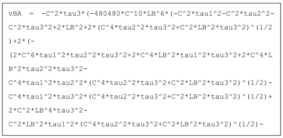
When rendered by Maple, the fragment of the solution looks like on Figure 3.

3.2.1. Verification of Results by Checking Numerical Consistency

In this situation we implemented numerical verification with 256 digits precision. Using equation (30) we substituted selected example numerical values for every unknown symbol needed to calculate the numerical value. We had to inspect up to 8 roots for every velocity trying to find the match to the assigned values and fortunately the results were exact to the 64 digits display limit as shown in Figure 4, which proves numerical consistency.

While big equations although appear correct solutions they are nearly useless and not rigorously proven.

3.2.2. Verification of Results via Back-Substitution

In nonlinear algebra, finding a solution is only half the battle; proving it is correct is the other half. We attempted to substitute large equations into the expressions (30), but the expanded raw expressions in tested cases were too large to simplify and prove the identinties of ${\tau }_1{\tau }_2{\tau }_3$ on two side of the equations. Attempts to automatically simplify the massive expression resulted in Maple fatal crashes due to the inssufficient 8 GB of RAM.

Fortunately another approach to thesystem (30) was taken. The original system was modified to the following by squaring both sides of the first and second equations:

$$\left\{\begin{array}{c}{\tau }_1^2={\displaystyle \frac{L_B^2(c^2-{v_{BA}}^2)(c^2-{v_{B1A}}^2)}{c^4{({-v}_{BA}+v_{B1A})}^2}} \\ {\tau }_2^2={\displaystyle \frac{L_B^2(c^2-{v_{BA}}^2)(c^2-{v_{B2A}}^2)}{c^4{({-v}_{BA}+v_{B2A})}^2}} \\ {\tau }_3={\displaystyle \frac{L_B\left(c^2-{v_{BA}}^2\right)}{c^2\left({-v}_{BA}{+v}_{B1A}\right)}}+{\displaystyle \frac{L_B\left(c^2-{v_{BA}}^2\right)}{c^2\left({-v}_{BA}{+v}_{B2A}\right)}}\end{array}\right.$$

(31)

We expected that vanishing square roots may help to get a simpler form of the solution on the expense of introducing more roots, which can be eliminated.

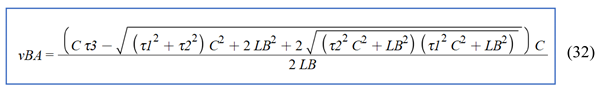
The improvement in time and size was a few magnitudes better and as a result, we have obtained a closed form short solution for v_BA, v_B1A, v_B2A with v_BA being of particular interest, which in the original Maple graphics was:

There were four roots for every velocity, each different. The only quick method to find the correct one was the identification by the numerical substitution. All expressions were tested based on the same times as in Figure 4, all accurate to 64 digits. The verification of identity of both sides of equations in system (31) by substitution of solved equations to the system appeared not possible symbolically because Maple failed to simplify to reduce complex expression to one symbol on the left hand of any equation in (31). However substitution of numerical values, again confirmed the identity check. For example:

${\tau }_1^2={\displaystyle \frac{L_B^2(c^2-{v_{BA}}^2)(c^2-{v_{B1A}}^2)}{c^4{({-v}_{BA}+v_{B1A})}^2}},$The returned computed values for each side of this equation were:

Not satisfied with the need of using numerics we approached the problem differently. After the substitution of solutions for v_BA, v_B1A, v_B2A into equations (31) we have obtained the system symbolically represented by:

$$\left\{\begin{array}{c}{\tau }_1^2=f_1({\tau }_1,{\tau }_2,{\tau }_3,L_B) \\ { \tau }_2^2=f_2({\tau }_1,{\tau }_2,{\tau }_3,L_B) \\ { \tau }_3=f_3\left({\tau }_1,{\tau }_2,{\tau }_3,L_B\right) \end{array}\right.$$

(33)

Each function was quite complex and simplify function was ineffective. However, we solved each equation, with respect to${\tau }_1$, ${\tau }_2, {\tau }_3$ in order. There were multiple roots, all respectively identical in the form: ${\tau }_1={\tau }_1, { \tau }_2={\tau }_2, { \tau }_3={\tau }_3$, 64 each for ${\tau }_1, { \tau }_2$ and 3 for ${\tau }_3.$ This analytical confirmation proves that the derived solution (32) are exact, rather than heuristic.

The simplified one-line formula (32) was truly a root of the original system. This 'closed-loop' verification proves that despite the immense complexity of the intermediate steps, the final result is an exact, error-free solution of the Tangherlini system in the specific case presented.

3.3. The Evaluation of the Results

It is certain that the three clocks scenario for the Lorenztian variant correctly represent the model presented in [1] and additionally the result included unpublished velocity expressions not considered in [1]. There is certainty that the derived system of equations (30) is also correct because the special case for v_BA=0 exactly matched the formula (2) and the derivation process is traceable and appears correct. Despite the initial inability to verify the analytical solution due to the massive size of velocity expressions, the numerical test at 256 digits precision produced accurate results to the 64 digits precision. However later approach to the system of equations led to remarkable result which was a short formula (32) verified as the correct solution finalising the initial objective of this study.

Summary:

• The algebraic proof of the solution correctness using Maple, has been achieved. Numerical test at a very high precision of 256 digits return exact expected results within the minimum of 64 digits precision for the calculated velocities.
• Furthermore, analytical validation was achieved by substituting solutions to the system of equations (31).
• Traceable derivations of equations from established theories.
• We are therefore convinced that the reality of absolute rest frame and absolute velocity is in principle proven pending 3D generalisation and experimental confirmation in the future.
• The fact that this is only verified for one special case in x-boost configuration does not put in doubt the general nature of our finding. The existence of this analytical solution implies a general solution for arbitrary velocity vector orientations, because this special case is the manifestation of laws of a general, nature acting in all axes configurations no matter how difficult is to obtain general solution in Tangherlini framework. It is hard to imagine that the absolute velocity solutions may exist only on axes aligned with absolute velocity vectors and not elsewhere. This is by analogy to the LT heavily exploited using x-boost configuration for education purposes, but there is no doubt any axes configuration that is more difficult to handle mathematically, would make relativistic effects disappear. A rigorous proof of this should be provided in the future for a full closure.

4. Discussion and Conclusions

4.1. Historical Perspective of the Absolute Velocity Problem

More than a century long scientific consensus is that absolute velocity cannot be detected or rather, there is no such thing. If we assume that the special case velocity solution derived here is between very high probability to certainty, then there are many questions to be answered

The detectibility of absolute motion is closely related to the concept of instantaneous signals. Superluminal and instantaneous signals have always been a contentious issue. The instantaneous signal is something that our common sense temporal intuition demands, yet generally this idea is regarded as unscientific. The consensus is that simultaneity is relative by nature, and the intuitive instantaneous perception, is a mistake according to Canales [4]. Einstein [5] described this mistake as a result of the failure to distinguish between what is simultaneously seen and what is simultaneously happening. However, he also made an interesting remark in 1911 [6] by addressing the concept of a signal propagating infinitely fast, allowing to define time, in contrast to time that was already defined in the 1905 relativity paper [7] (described in the most recent English translation [3]).

The instantaneous temporal relation between distant events is commonly understood as ‘Now.’ This was officially abolished by Eddington [8]. He stated that there was no such thing like absolute ‘Now’, but only the multitude of relative ‘Nows’ different for every observer. However, this concept was hard to abandon even by some prominent physicists. According to Jammer [9] quoting Rudolf Carnap, the problem of ‘Now’ seriously worried Einstein. Without expanding on the full complexity of this problem it can be noticed, that the instantaneous temporal relation introduced some uncertainty in the minds of other physicists such as Bell [10], who insisted on the existence of a mechanism by which the setting of a measuring device influences the reading on another instrument at any distance, and the signal involved must be instantaneous, implying that the underlying theory cannot be Lorentz invariant.

The reality of the instantaneous signal is in fact the existence of a mathematical limit of the infinite set of superluminal signals EOMs with forever increasing velocity. This could as well be intuitively dismissed. Even the intuition of a creative mind allowing the instantaneous perception of the whole universe at once, may find it hard to picture something like a signal moving from here to a distant galaxy or beyond in no time, let alone the reflected signal returning at the exact moment when it is emitted. Instantaneous signal appears to be a violation of causality based on a simple local commonsense reasoning. At the time of emission one can expect the signal to be delivered where it isn’t, so how it returns now from where it wasn’t? Mathematics however, can be more forgiving than the imagination. Instantaneous signal is the limit of all signals sent in the same direction with ever increasing velocity. There is no a fixed infinity number it is an open ended series of numbers with no maximum hence our intuitive non-causality concerns can be defeated by the fact that such situation can never happen and the succession of emission-return event is preserved no matter how short. The unreachable limit means coexistence, which may not necessarily be probed by signals. This opinion however, is naturally opened for challenge as any scientific subject,

Inability to find instantaneous signals in nature prevented generations of philosophers and scientists defining the same time in remote locations. The blocking issue was the famous circularity when two clocks at different locations should indicate the same time simultaneously, while ‘simultaneously’ meant at the same time. Einstein [7] solved the problem assuming the same one-way velocity of light independent on the motion of the observer and the direction of its motion, against common sense, inspired by Michelson and Morley experiments [11] according to which the round-trip average speed of light was constant. However, this was not one-way velocity. With the assumed isotropy and additional postulates Lorentz Transformation was derived in a new context by Einstein and the STR was born. At about the same time Poincaré [12] published one of the earlier (June 5 1905) versions of the Postulate of Relativity as follows:

It seems that this impossibility of experimentally demonstrating the absolute movement of the Earth is a general law of Nature; we are naturally inclined to admit this law, which we will call the Postulate of Relativity, and to admit it without restriction. Whether this postulate, which has so far been in agreement with experience, should be confirmed or refuted later by more precise experiments, it is in any case interesting to see what the consequences may be.[1]

Unlike in Einstein’s systematic derivation approach this formulation seems to assume a-priori the absence of absolute movement of the Earth, without mentioning one-way velocity. The uncertainty expressed in the last sentence may explain the long desire to detect the ether and absolute motion relative to it. Michelson and Morley [11] concluded after experiments that any relative motion between the earth and the ether must at least be very small.

Absolute velocity concept and variable one-way velocity of light have become obsolete in mainstream physics. Some researchers continued seeking methods to overcome the burden of instantaneous synchronization preventing one-way velocity measurement. Several examples can be found in publications of Mansouri and Sexl [13], Selleri [14], [15], Tangherlini [16], Spavieri, Gillies and Haug [17], just to mention a few. The focus is often on rotating frames and the well known experimentally confirmed Sagnac effect. This situation is still not ideal because the general remote clock synchronisation problem for inertial systems in rectilinear uniform motion has not been conclusively solved so far in the form of specific velocity formula, to the best knowledge at the time of writing.

Tangherlini himself tried to reason about the possibility or otherwise of detecting absolute motion based on his theory.

Starting with relative velocity (e.g. of clock C1 in frame B), Tangherlini concludes that if two distant clocks are not absolutely synchronised, it is not possible to calculate the one-way relative velocity, because velocity is defined non-locally so there is no way of finding the time of arrival in terms of the time of departure. [2] p58. This is not true in the context of our finding because three clock measurement scenario provides theoretical alternative without clock synchronisation as they only measure their own proper time between two events and we see relative velocity expressions in equations (28) from which the velocity v₁ or v₂ can be calculated. This is possible now, because no one before Unruh[2] seems to have considered this possibility.

In another place [2] p73-74 Tangherlini sees a sufficient condition to be able to detect the absolute motion in a moving frame (e.g. B in our case) that there must be at least one other signal propagating with constant absolute velocity with speed not equal to c, in particular, when (as in our case) the second speed vB1A> vBA. However, no closed form solution or measurement method demonstrating this possibility is provided.

In the final Conclusions section of [2] p101, Tangherllini’s summary conveys the following:

In examples presented in the doctoral thesis, absolute velocity always cancels out when measurements are performed “in the usual manner”. This means methods depending on the absolute synchronization of separated clocks. In our case the three clock measurement method is not “in the usual manner” therefore the solutions could be found.

4.2. Conclusions

• Tangherlini prediction of the possibility of detecting absolute velocity were confirmed by our solution because the three clocks scenario did not require separated synchronized clocks to define the velocity which was not “in the usual manner”.

2.

The special case solution we obtained from equations (31), is a manifestation of a general law of nature like Einstein’s simplified SRT’s first findings were the manifestation of GR laws. This yielded relatively simple expression for absolute velocity of the base platform:

3.

Although finding absolute velocity may appear to undermine the STR, this is not the case. The Einstein’s convention is consistent with the underlying fundamental laws by which the average speed of round trip of light is constant and the theory is verifiable within the Einstein - Poincaré synchronized clock ensembles, but not necessary reflecting the synchrony perceived by humans, deemed absolute. The convention takes absolute velocity out of scope, by but it cannot deny or confirm its existence ruled out by definition, so no contradiction with Tangherlini theory. However, some relativistic narratives in literature having no real effect on scientific results may not be accurate. In this view the Poincaré formulation of the Postulate of Relativity was an unproven inference and now becomes obsolete; however, it was ‘mostly right’, reflecting the state of knowledge in early 20^th century. Einstein’s postulates appear to be not affected by our findings.

4.

The results presented here demonstrate that nature did not conspire but the absolute velocity of an inertial frame is not hidden but at least is a mathematically accessible quantity when using a three-clock measurement protocol advocated by Matsas et al. [1] , we have shown that Tangherlini’s 1958 theory is both testable and internally consistent. The single, elegant analytical solution represents a significant simplification of the kinematics of preferred frames. Future experimental verification and extension of the presented model could resolve the debate regarding the existence of a preferred frame, moving it from the realm of philosophical interpretation into the domain of empirical measurement."

5.

We hope the results of this work will trigger additional research leading to finding a practical method to measure absolute velocities with high accuracy, which this special case cannot support due to the unknown orientation of the absolute velocity vector needed to be aligned with the coordinate system x-axis.

6.

The unusual nature of the discovery of absolute velocity reflects the long standing view of late Jose G. Vargas [18]: ” there is more to structure in special relativity than meets the eye.”

References

- Matsas, G.E.A.; Pleitez, V.; Saa, A.; Vanzella, D.A.T. The number of fundamental constants from a spacetime-based perspective. Sci. Rep. 2024, 14, 1–12. [Google Scholar] [CrossRef] [PubMed]
- Tangherlini, F.R. The Velocity of Light in Uniformly Moving Frame- PhD Disertation Stanford University1958. The Abraham Zelmanov Journal 2009, vol. 2, 44–110. [Google Scholar]
- Einstein, A. On the Electrodynamics of Moving Bodies," in The Collected Papers of Albert Einstein. (English). Princeton: Princeton University Press. 1989, Volume 2, 140. Available online: https://einsteinpapers.press.princeton.edu/vol2-trans/154.
- Canales, J. Einstein, Bergson, and the Experiment that Failed: Intellectual Cooperation at the League of Nations. MLN 2005, 120, 1168–1191. [Google Scholar] [CrossRef]
- Einstein, A. Physics and reality. J. Frankl. Inst. 1936, 221, 349–382. [Google Scholar] [CrossRef]
- Einstein, A. ""Discussion" Following Lecture Version of "Theory of Relativity"," in The Collected Papers of Albert Einstein. In The Swiss Years Writings 1909-1911 (English translation supplement); Princeton University Press: Princeton, 1994; Volume 3, p. 353. Available online: https://einsteinpapers.press.princeton.edu/vol3-doc/478.
- Einstein, A. Zur Elektrodynamik bewegter Körper. Annalen der Physik, Band 17 1905, vol. 17, 1905. Available online: https://dn790008.ca.archive.org/0/items/zurelektrodynami00aein/zurelektrodynami00aein.pdf. [CrossRef]
- Eddington, A.S. The Nature of the Physical World; Cambridge University Press: Cambridge, 1929; Available online: https://www.gutenberg.org/cache/epub/72963/pg72963-images.html.
- Jammer, M. Concepts of Simultaneity: From Antiquity to Einstein and Beyond; Johns Hopkins University Press: Baltimore, 2006. [Google Scholar]
- Bell, J.S. On the Einstein Podolsky Rosen paradox. Phys. Phys. Fiz. 1964, 1, 195–200. [Google Scholar] [CrossRef]
- Michelson, A.A.; Morley, E.W. On the relative motion of the Earth and the luminiferous ether. Am. J. Sci. 1887, s3-34, 333–345. [Google Scholar] [CrossRef]
- Poincaré, H. Sur la dynamique de l'électron. Rendiconti del Circolo Matematico di Palermo 21, 1906, 129–176 1906, vol. 21, 129–176. [Google Scholar] [CrossRef]
- Mansouri, R.; Sexl, R.U. A test theory of special relativity: I. Simultaneity and clock synchronization. Gen. Relativ. Gravit. 1977, 8, 497–513. [Google Scholar] [CrossRef]
- Selleri, F. Noninvariant one-way speed of light and locally equivalent reference frames. Found. Phys. Lett. 1997, 10, 73–83. [Google Scholar] [CrossRef]
- Selleri, F. Noninvariant one-way velocity of light. Found. Phys. 1996, 26, 641–664. [Google Scholar] [CrossRef]
- Tangherlini, F.R. Galilean-Like Transformation Allowed by General Covariance and Consistent with Special Relativity. J. Mod. Phys. 2014, 05, 230–243. [Google Scholar] [CrossRef]
- Spavieri, G.; Gillies, G.T.; Haug, E.G. The Sagnac effect and the role of simultaneity in relativity theory. J. Mod. Opt. 2021, 68, 202–216. [Google Scholar] [CrossRef]
- Vargas, J.G. U(1) ×SU(2) from the tangent bundle. In J. Phys.: Conference Series 474, 2013 doi:10.1088/1742-6596/474/1/012032, pp. 1-17.
- Poincaré, H. The Value of Science; Science Press: New York, 1907. [Google Scholar]
[1] Translation from [12] by Google Translate. |
[2] Bill Unruh undisclosed private communication according to [1]. |
[3] We used the observation of Poincare that absolute space is not definable and has no features with coordinates so the only way to bootstrap the derivation is to assume that at time 0 some abstract coordinate system in A is momentarily aligned with the moving one: “absolute space is nonsense, and it is necessary for us to begin by referring space to a system of axes invariably bound to our body (which we must always suppose put back in the initial attitude).” [19] Absolute space then has no role other than being a container of inertial systems only as far as this simple linear algebra model is concerned. |
Figure 1.
The three clocks scenario (angles no to scale).
Figure 2.
Three clocks scenario in system B in absolute space (angles not to scale).
Figure 3.
Fragment of Maple solution as rendered by Maple.
Figure 4.
Numerical validation of absolute velocity solution. The av[i] are selected roots holding the expected velocity values. C1, C2, C3 hold expressions of equations (30).
Disclaimer/Publisher’s Note: The statements, opinions and data contained in all publications are solely those of the individual author(s) and contributor(s) and not of MDPI and/or the editor(s). MDPI and/or the editor(s) disclaim responsibility for any injury to people or property resulting from any ideas, methods, instructions or products referred to in the content. |
© 2026 by the author. Licensee MDPI, Basel, Switzerland. This article is an open access article distributed under the terms and conditions of the Creative Commons Attribution (CC BY) license.
Copyright: This open access article is published under a Creative Commons CC BY 4.0 license, which permit the free download, distribution, and reuse, provided that the author and preprint are cited in any reuse.