Precise Analysis and Prediction of Active Earth Pressure for Retaining Walls Based on Explainable Machine Learning

1. Introduction

The precise estimation of lateral earth pressure is critical for the structural analysis and design of retaining walls, and remains a persistent challenge in geotechnical engineering [1,2,3,4]. Despite the simplicity offered by classical theories (e.g., Rankine, Coulomb) in terms of analysis due to their assumption of a state of ultimate limit equilibrium and a linear pressure distribution, significant deviations have been demonstrated between theoretical predictions and actual measurements, as evidenced by extensive experimental and field research [5,6,7]. In practice, retaining wall movements (e.g., translation, rotation about the base, or rotation about the top [8]) generally occur under non-limit conditions, i.e., when the soil has not yet achieved a state of plastic equilibrium. This phenomenon is further complicated by the soil arching effect, which induces a pronounced nonlinear earth pressure distribution. This distribution is highly sensitive to wall displacement mode and magnitude [9]. Therefore, a comprehensive understanding of the intricate, displacement-coupled nonlinear behavior of earth pressure under non-limit conditions is imperative for the advancement of the scientific design and safety evaluation of retaining structures.

Conventionally, the investigation of earth pressure behavior has been undertaken through analytical derivations, model testing, and numerical simulations. Handy [10] and subsequent researchers [11,12] proposed formulations that deviated from classical linear assumptions by building upon soil arching theory. Various soil arch profiles have been incorporated into these analytical models to capture non-limit state behavior [13,14,15]. While model tests do provide high-fidelity data [16,17,18,19,20], they are inherently labor-intensive and cost-prohibitive. Consequently, numerical approaches have gained significant attraction in the field [21,22]. Specifically, a Finite Element Analysis (FEA) has been widely utilized to characterize the development of failure surfaces and continuous stress evolution [23,24,25,26]. In addition to these continuum approaches, the Discrete Element Method (DEM) has been effectively employed to unveil granular-level distributions and nonlinear pressure coefficients [27,28]. Moreover, a substantial body of research has examined the variation of earth pressure within the framework of the finite soil displacement concept [29,30,31,32]. Despite these advancements, numerical methods frequently necessitate intricate constitutive models and substantial computational overhead, thereby impeding their responsiveness in real-time engineering assessments.

In recent years, machine learning methods have been increasingly applied to the study of retaining wall structures. The utilization of these techniques results in a number of notable advantages, including but not limited to rapid computation, high accuracy, low cost, and the inherent capability to automatically capture complex nonlinear relationships. For instance, Shin et al. [33] employed machine learning to predict the horizontal displacement of soil-anchored retaining walls, systematically examining the influence of data standardization methods and data splitting strategies on model performance. Zhang et al. [34] demonstrated the feasibility of using multivariate adaptive regression splines (MARS) as an alternative to backpropagation neural networks (BPNN) for addressing geotechnical engineering problems. Mishra et al. [35] employed a range of machine learning models, including emotional neural networks (ENN), MARS, and SOS–LSSVM, to predict the safety factors of retaining walls for structural reliability analysis. In the domain of design optimization, the research by Aydın et al. [36] predicted optimal retaining wall dimensions and associated costs based on wall height (H) and surcharge load (q) parameters. Linear regression, ridge regression, and Lasso regression were employed as base learners in a multi-output regression framework. Similarly, Bekdaş et al. [37] conducted a comparative analysis of the performance of four algorithms, including random forest, for predicting the optimal base width of retaining walls.

However, the application of the aforementioned ML techniques to retaining wall analysis is also subject to certain limitations. Firstly, from the perspective of engineering application, existing studies frequently do not directly address the substantial problem of earth pressure determination. Secondly, from a methodological perspective, the extant body of research rarely addresses the critical challenge of model interpretability in machine learning. Although Bekdaş et al. [37] employed SHAP scatter plots for the purpose of visualizing the relationship between design features and optimal wall dimensions, they did not provide explicit physical explanations from the perspective of earth pressure mechanics. The emphasis, instead, remained predominantly on the predictive accuracy and computational efficiency of the models. A prevalent trend in current machine learning practice, as evidenced by the notion that tree-based models can "tolerate redundant features," involves pursuing marginal gains in accuracy through feature stacking. This methodological approach frequently obscures the underlying geomechanical logic, which can further diminish physical interpretability. Consequently, despite an increasingly growing attention to machine learning applications in civil engineering, the inherent "black-box" nature of purely data-driven models obscures the physically meaningful relationships between input features and target variables [38]. This deficiency in interpretability persists as a significant impediment to their broader adoption in practical engineering applications.

The objective of this study is to address the limitations inherent in classical theories of active earth pressure and the prevailing challenges regarding interpretability in machine learning applications. To address this knowledge gap, the present study proposes a key feature refinement strategy that utilizes collinearity analysis to prioritize the most influential physical descriptors. The identification of a concise set of five fundamental parameters, including displacement mode and relative displacement magnitude, has been demonstrated to facilitate a balanced equilibrium between the predictive accuracy and physical complexity. The CatBoost/SHAP framework is subsequently employed to reveal the nonlinear influence of five proposed key physical parameters on the coefficient of earth pressure. Finally, a graphical user interface (GUI) software tool has been developed that is designed to be user-friendly and facilitate the practical engineering application of the proposed model.

2. Materials and Methods

2.1. Data Integration and Fundamental Features

2.1.1. Data Sources

A machine learning database is established utilizing existing experimental data on earth pressure from retaining wall model tests reported in the literature. Potential sources for earth pressure data include field testing, model testing, and numerical simulation. Field testing often faces challenges in accurately measuring wall displacement and typically provides limited data points. Numerical simulation, while useful, may introduce distortions due to idealized constitutive assumptions. In contrast, model testing allows for the controlled simulation of various displacement magnitudes under predefined modes. Following a comprehensive literature review, studies with incomplete experimental data [17,39] are excluded. Consequently, data from four publications [16,18,19,20] are identified and integrated as the primary sources for constructing the machine learning database in this study.

2.1.2. Data Cleaning

To obtain accurate earth pressure data, the data points are first extracted from the earth pressure curves presented in the literature using digital tools and converted into numerical values, resulting in a total of 1021 raw samples. The sample sizes collected from each source are as follows: 234 samples from Fang et al. [16], 703 from Rui et al. [18], 75 from Shi et al. [19], and 9 from Yao et al. [20]. Subsequently, the collected raw dataset undergoes a cleaning process. Since the model tests by Rui et al. [18] employed a single soil type (sand with a unit weight of 18.13 kN/m³ and an internal friction angle of 42.3°), their sample size is substantially larger than those from other sources. To improve dataset balance, 378 samples from this source are removed by thinning. Additionally, six samples corresponding to a relative translation of 0.0027 and six samples for a rotational displacement about the wall base of 0.00896 from Rui et al. [18] are excluded for independent verification in the subsequent GUI program. Furthermore, analysis identifies one test condition in Fang et al. [16]—where the earth pressure coefficient near the wall crown reached 1.95 during rotation about the crown—as a significant outlier compared to other samples, and it is therefore removed. Following this cleaning procedure, a final set of 630 samples is selected for machine learning in this study.

2.1.3. Basic Features and Target Variable

Based on the governing mechanisms of earth pressure and the information available from the source literature, five physical parameters are selected as the fundamental input features: soil unit weight, internal friction angle, soil depth, wall displacement mode, and wall displacement magnitude. The earth pressure coefficient K is designated as the target variable. It is defined by the following equation:

$$K={\displaystyle \frac{p}{\gamma Z}}$$

(1)

where p is the horizontal earth pressure behind the wall, γ is the unit weight of the backfill soil, and Z is the soil depth measured from the wall crown. Specifically, the input feature for soil depth is expressed as the relative depth Z/H, and wall displacement as the relative displacement ∆/H, where H is the wall height and ∆ is the absolute displacement at the wall crown. This normalization facilitates consistent analysis of earth pressure, depth, and displacement across varying wall dimensions. The preliminarily selected fundamental features and the target variable are summarized in Table 1.

The data presented in Table 1 consist of two types: numerical variables (denoted by N) and categorical variables (denoted by C). The displacement mode is represented as a categorical variable with three distinct modes: translation (T), rotation about the wall top (RT), and rotation about the wall base (RB). All remaining features are numerical variables.

2.2. Justification for CatBoost Selection

The CatBoost algorithm [40,41,42] is employed directly as the core solver for the prediction model in this study. This selection is based primarily on three considerations pertaining to the characteristics of geotechnical engineering data:

a) Native support for categorical features: The earth pressure coefficient is significantly influenced by discrete categorical features, such as the displacement mode. CatBoost’s unique ordered boosting and built-in handling mechanisms for categorical variables allow such features to be processed directly and efficiently. This avoids the issues of feature space expansion and potential information distortion associated with one-hot encoding, which is required by many other algorithms (e.g., artificial neural networks (ANN) [43,44,45] or support vector regression (SVR) [46,47]).

b) Robustness against overfitting with small samples: Owing to the inherent difficulty in collecting geotechnical model test data, the dataset in this study is limited in size. CatBoost effectively mitigates overfitting during training by calculating gradient statistics on permutations of the data, thereby demonstrating strong generalization capability and robustness on small- to medium-sized datasets.

c) Validation based on prior research: In previous work by the authors focusing on the prediction of ultra-high-performance-concrete (UHPC) properties [48], an extensive benchmarking study was conducted. The results demonstrated CatBoost’s superior performance and stability in handling complex, nonlinear regression problems involving material and structural parameters.

Therefore, the focus of this study is shifted from conventional algorithmic comparisons to ensuring the model’s physical consistency and engineering applicability. Rather than repeating redundant algorithm screening procedures, CatBoost is directly selected as the core algorithm for constructing the intelligent design tool. Furthermore, research by the authors and others [48,49] indicates that ensemble learning algorithms, including CatBoost, can achieve satisfactory predictive accuracy even with default hyperparameters. Consequently, no explicit hyperparameter tuning is performed on the CatBoost model in this work.

2.3. Cross-Validation and Independent Testing

To ensure an objective and reliable evaluation of the model's generalization performance, an equal-frequency stratified sampling strategy is employed. This strategy partitions the dataset evenly based on the numerical distribution of the target variable, the earth pressure coefficient K. First, the entire dataset is split into a training set and an independent test set at an 80:20 ratio. To maximize the use of the limited sample data and optimize the model, a 5-fold cross-validation procedure is applied exclusively to the training set. The independent test set (i.e., the reserved 20% of data) is kept strictly isolated and is used solely for the final validation of model performance, thereby providing an unbiased estimate of its predictive capability on unseen data. This rigorous separation effectively prevents data leakage and ensures the robustness of the model evaluation.

2.4. Model Evaluation Metrics

The selection of model evaluation metrics is crucial for objectively assessing model performance. This study employs three widely recognized statistical indicators to conduct a multidimensional quantitative evaluation of the predictive accuracy of the CatBoost regression model [50], including the Coefficient of Determination (R²), Root Mean Squared Error (RMSE), and Mean Absolute Error (MAE). R² measures the model's ability to explain data variation; RMSE and MAE respectively, measure the average magnitude of prediction errors, with the former being more sensitive to large errors.

2.5. Model Interpretation Strategy

The SHapley Additive exPlanations (SHAP) framework is employed to interpret the predictions of the machine learning model. Rooted in cooperative game theory and Shapley values, SHAP provides a theoretically grounded, additive method for explaining the output of complex, black-box models. It frames each prediction as a game where features are players, and their contributions to the prediction (relative to a baseline) are fairly allocated, ensuring both local accuracy and global consistency [51,52,53,54]. In this study, SHAP is utilized in three progressive stages: first, global feature importance is assessed using SHAP bar plots and violin plots. Second, SHAP dependence plots are analyzed to elucidate the nonlinear relationships between individual features and the earth pressure coefficient. Finally, SHAP interaction analysis is conducted to reveal the underlying mechanisms and interactive effects that govern the nonlinear distribution of earth pressure.

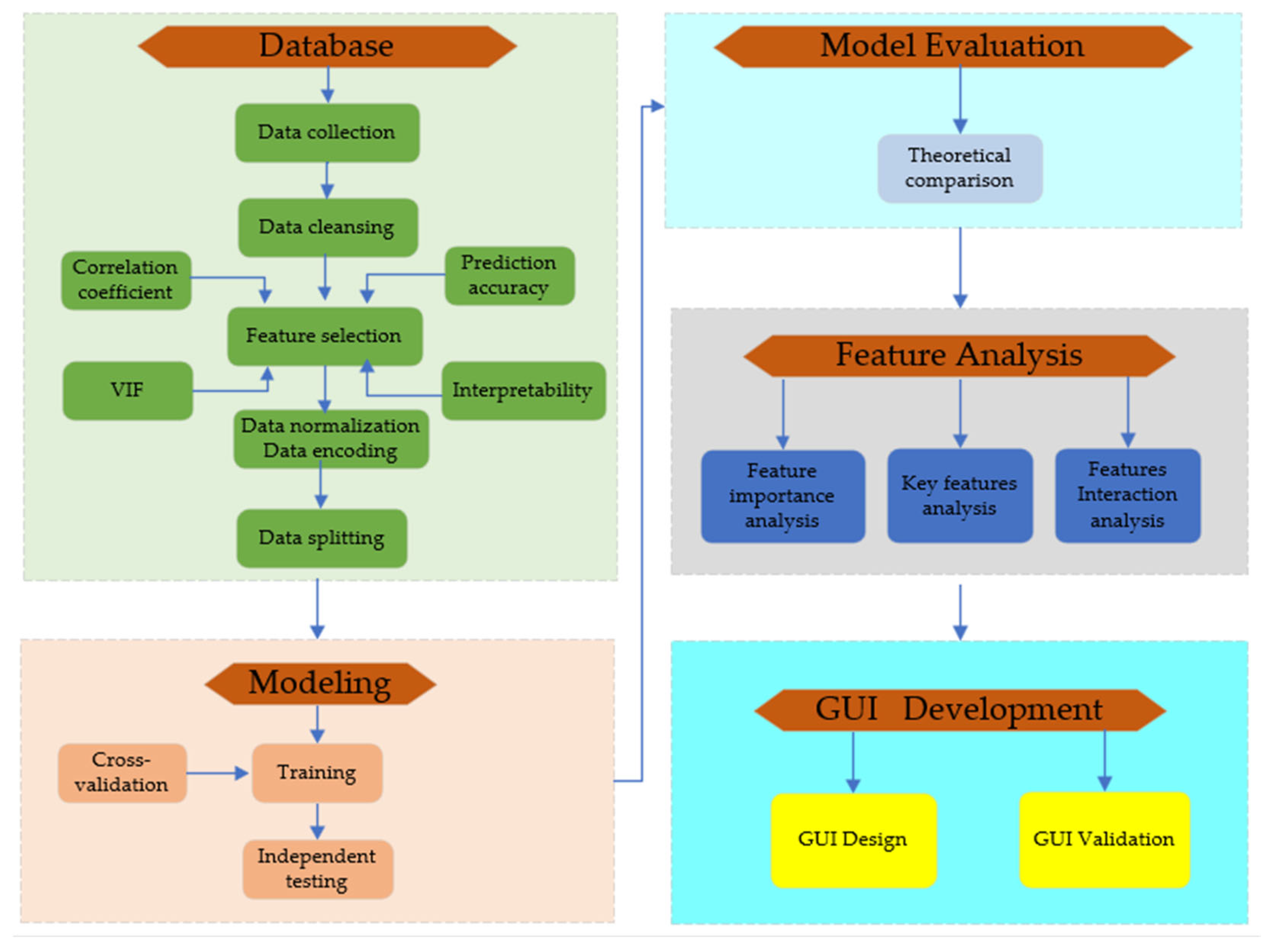
2.6. Research Framework

The overall research framework is illustrated in Figure 1. The workflow comprises the following key steps:

a) Database establishment: A database is constructed using experimental data from existing literature on earth pressure in retaining wall model tests. The process involves data collection, cleaning, feature selection, normalization, encoding, and segmentation. Feature selection is guided by a “key feature refinement strategy based on collinearity analysis”, which is detailed in Chapter 3.

b) Model development and evaluation: The CatBoost algorithm is employed to train the prediction model using its default hyperparameters. Model training incorporates a 5-fold cross-validation procedure. Upon completion of training, the model's final performance is evaluated on a strictly held-out independent test set.

c) Performance benchmarking: The predictive accuracy of the developed machine learning model is systematically compared with results derived from classical theoretical earth pressure calculations.

d) Model interpretation: To address the interpretability challenge inherent in data-driven models, the SHAP framework is utilized. It provides both visual and quantitative explanations, elucidating the influence of various input features on the earth pressure coefficient and revealing their underlying physical relationships.

e) Tool implementation: A user-friendly graphical user interface (GUI) program is developed. This tool enables users to input key parameters, including wall height, backfill unit weight, internal friction angle, displacement mode, and relative displacement, and rapidly obtain visualizations of the resulting earth pressure distribution and the total lateral force acting on the retaining wall.

3. Key Feature Selection and Refinement

3.1. Attempts at Expanding Feature Sets

Feature selection critically influences both the accuracy and interpretability of machine learning predictions. An insufficient feature set may omit crucial physical information, compromising predictive precision. Conversely, an excessively large set can increase model complexity, leading to overfitting and obscuring physical interpretability. To ensure the model adequately captures the underlying physical mechanisms and established engineering knowledge relevant to earth pressure prediction, an expanded set of engineering features is introduced, supplementing the five fundamental physical parameters (γ, φ, Z/H, Δ/H, and DM). The objective is to incorporate information from limit state theory and to better describe coupled stress-displacement effects. Specifically, two additional features are proposed:

a) The Rankine active earth pressure coefficient, Ka(φ), calculated based on the soil's internal friction angle (φ).

b) An interaction term, I = (Z/H) · (Δ/H), designed to quantify the coupling effect between normalized soil depth and normalized wall displacement.

The inclusion of these features enriches the initial feature set with more comprehensive engineering prior knowledge, establishing a necessary basis for the subsequent evaluation of feature redundancy and collinearity.

3.2. Multicollinearity Analysis and Quantification

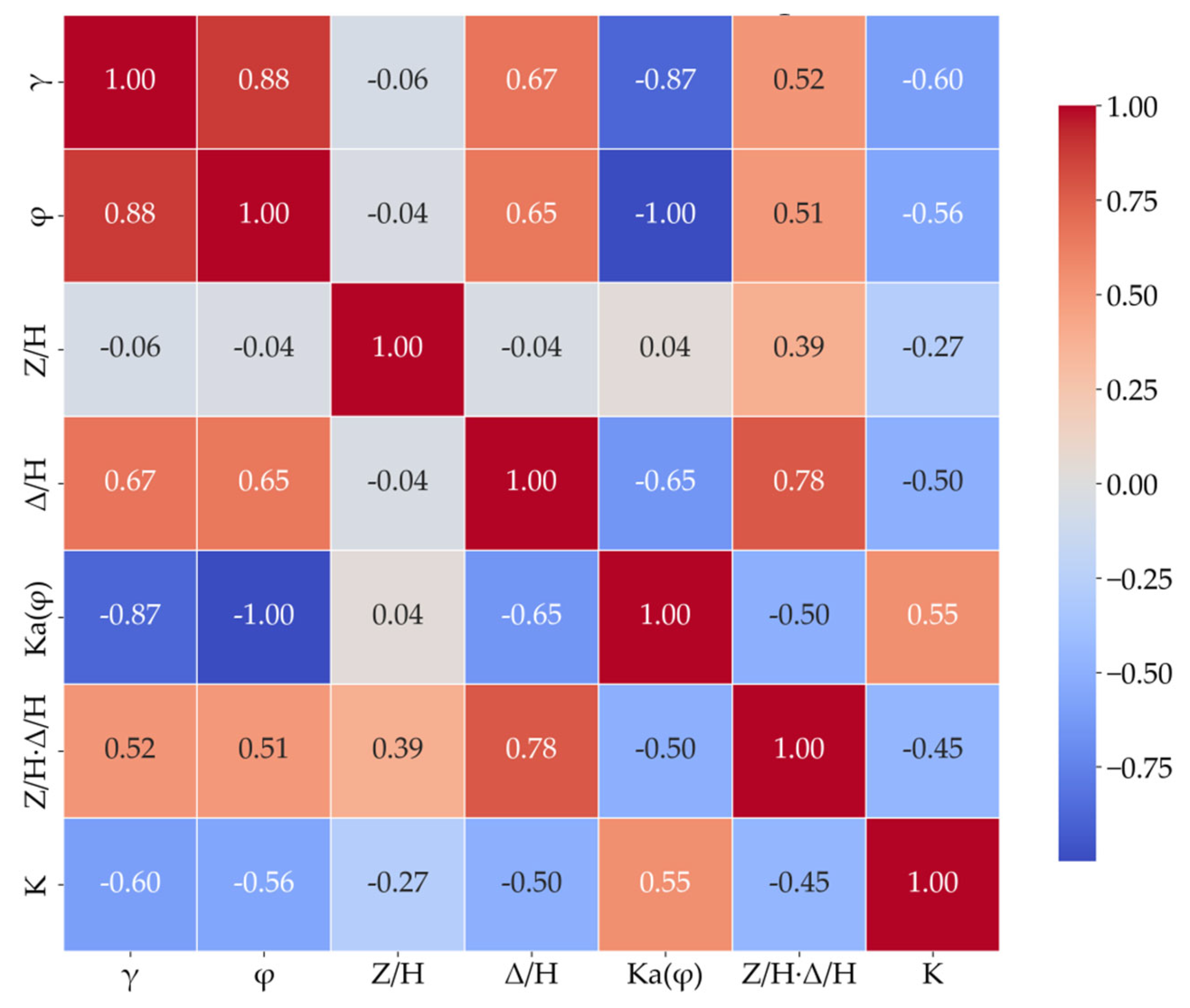
To identify the optimal feature set for model development, three distinct sets are constructed from the pool of seven candidate features (i.e., the five basic features plus the two extended features). Set 1 contains only the five basic features. Set 2 comprises the basic features plus the Rankine active earth pressure coefficient, Ka(φ). Set 3 includes all features from Set 2 plus the interaction term I. These three sets are compared and evaluated based on four criteria: inter-feature correlation coefficients, the variance inflation factor (VIF), model prediction accuracy, and model interpretability.

Figure 2 presents the Pearson correlation coefficient heatmap for Feature Set 3. Positive and negative values indicate positive and negative linear correlations, respectively, with darker colors representing stronger correlations (higher absolute values). As shown in the figure, the correlation coefficient between Ka(φ) and φ is -1.0, indicating a perfect negative correlation as dictated by the Rankine formula. The correlation between the interaction term I and Δ/H is 0.78, suggesting a high degree of collinearity. Furthermore, a significant correlation (0.88) is observed between the two fundamental soil properties, γ and φ. This relationship can be partly attributed to the characteristics of sandy soils, where a higher unit weight often corresponds to lower porosity, denser particle packing, and consequently a higher internal friction angle. It may also reflect the inherent property correlations within the specific soil samples comprising the database.

Table 2 presents a comparative analysis of the variance inflation factor (VIF) across the different feature sets. For an independent variable x_j in a regression model, its VIF is defined as:

$${VIF}_j={\displaystyle \frac{1}{1-R_j^2}}$$

(2)

where $R_j^2$ is the coefficient of determination obtained by regressing x_j on all other independent variables. A VIF value of 1 indicates no linear correlation with other predictors (i.e., no multicollinearity). Values between 1 and 5 generally suggest mild and acceptable collinearity, whereas values exceeding 5 indicate severe multicollinearity that warrants further attention.

As shown in Table 2, when Ka(φ) is included in the feature set, its VIF with respect to φ reaches approximately 2000, indicating severe multicollinearity. This result is expected because Ka(φ) is a deterministic function of φ (with a Pearson correlation coefficient of −1.0), making it redundant for predictive modeling.

An ablation study is conducted to evaluate and compare model performance under different feature combinations (Table 3). The evaluation metrics presented in Table 3 are obtained from the independent test set after model training using five-fold cross-validation. The results indicate that the model utilizing only the five basic features achieves satisfactory generalization performance. The introduction of either Ka(φ) or the interaction feature I leads to an improvement in test-set performance; however, this improvement is marginal (ΔR2<0.006).

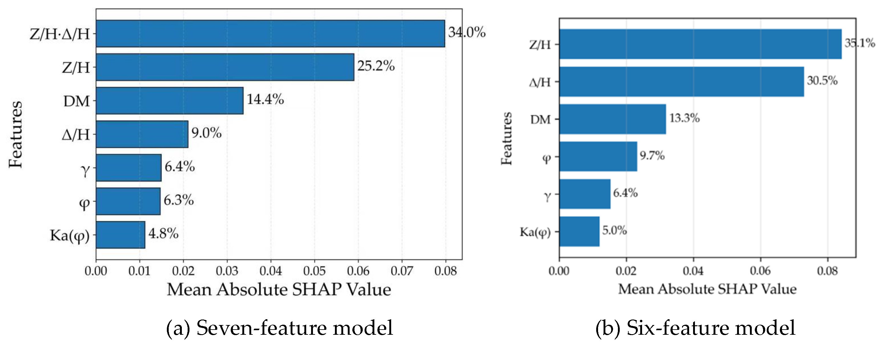
By ranking feature importance based on SHAP values in both the seven-feature and six-feature models (see Figure 3), differences in the interpretative contribution of each feature can be further observed. Although the correlation coefficient between the interaction term I (i.e., Z/H·Δ/H) and other features is not particularly high, and its variance inflation factor (VIF = 4.62) falls within an acceptable range, Figure 3(a) shows that its contribution proportion ranks highest among all features, reaching 34.0%. This finding clearly contradicts established physical interpretations of earth pressure behavior. While the importance ranking in Figure 3(b) appears more reasonable, the correlation heatmap presented earlier reveals a strong collinearity between Ka(φ) and φ. Therefore, the introduction of extended features offers only marginal improvement in predictive accuracy, while their high multicollinearity severely distorts SHAP’s assessment of the contributions from fundamental physical parameters. As previously emphasized, for machine learning applications in engineering, the importance of interpretability is no less than that of predictive performance. Consequently, this study concludes that the simplified set of five fundamental features listed in Table 1 should be adopted as the optimal model inputs.

4. Results and Mechanism Analysis

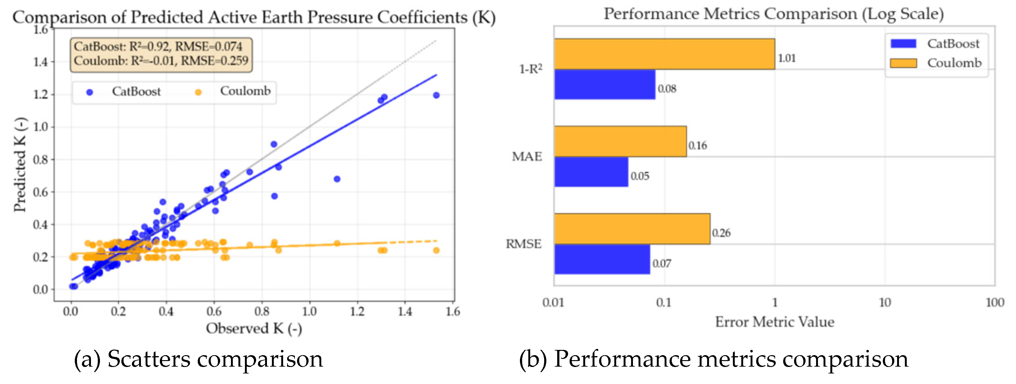
4.1. Model Performance Evaluation and Theoretical Comparison

In this study, the CatBoost algorithm is employed to train the model using the simplified five-feature set under default hyperparameters. Model performance is evaluated on an independent test set and subsequently compared with earth pressure coefficients calculated using Coulomb’s classical theoretical formula. A comparative visualization of the results is presented in Figure 4. It should be noted that, as the wall–soil interface friction angle was not reported in the source literature of the original dataset, the Coulomb theoretical calculations assum this angle to be 0.5 times the internal friction angle of the backfill.

As shown in Figure 4(a), the scatter plot of the machine learning predictions clusters closely along the 45° line of perfect agreement, with a narrow dispersion, indicating high predictive accuracy. In contrast, the scatter points derived from Coulomb's theoretical calculations are predominantly distributed horizontally within the range of 0.2–0.3. Apart from a minor overlap with the 45° line in the lower value region (around 0.2), most points exhibit a significant deviation, indicating a substantial discrepancy between the theoretical predictions and the measured data. Figure 4(b) provides a quantitative comparison of the two approaches using three metrics (1−R², MAE, and RMSE). The results demonstrate that the machine learning model developed in this study achieves markedly higher accuracy than the traditional theoretical formula under non-limit states and complex displacement modes.

4.2. Feature Importance Analysis

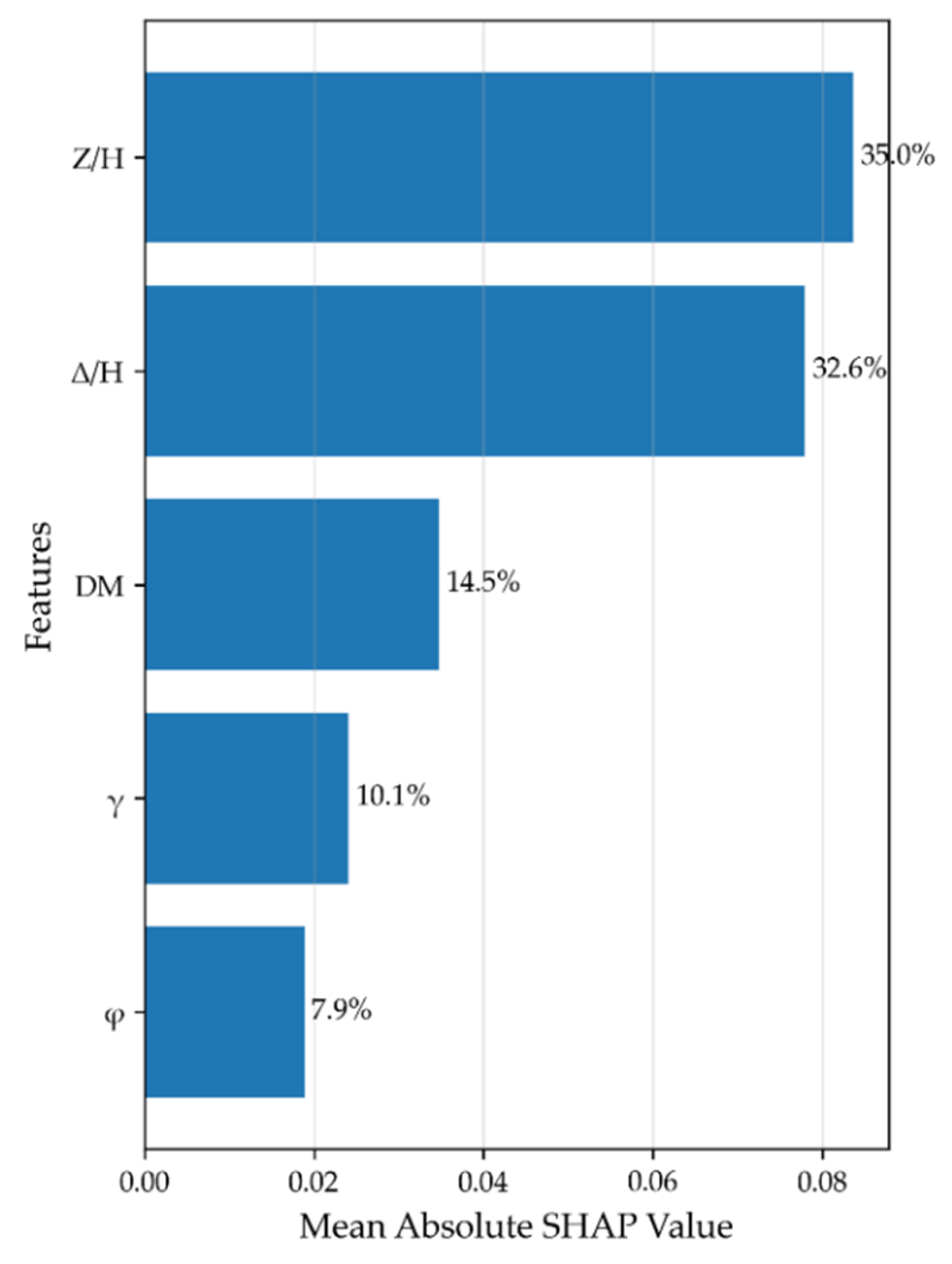
Figure 5 presents the feature importance ranking derived using the SHAP framework under the default hyperparameters of the CatBoost model. The horizontal axis corresponds to the mean absolute SHAP value for each input feature, while the vertical axis lists the features in descending order of their contribution to the model output. The numerical label on the right side of each bar indicates its contribution rate, calculated as the proportion of its mean absolute SHAP value relative to the sum across all features.

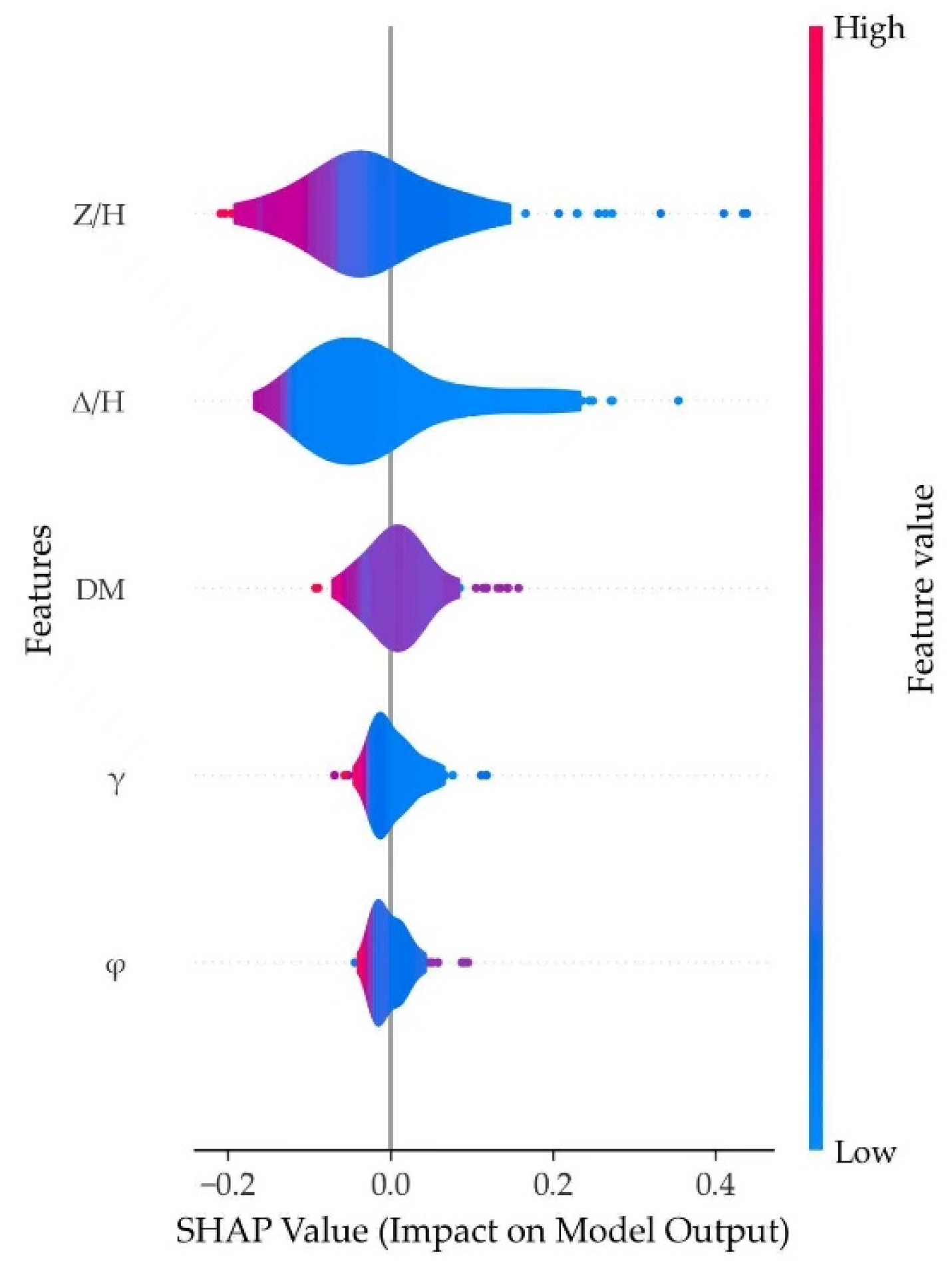
Figure 6 displays the SHAP summary plots in the form of violin plots for each feature. The horizontal axis represents the SHAP value (negative on the left, positive on the right), and the vertical axis maintains the same feature order as in Figure 5. The width of each violin reflects the kernel density estimation (KDE) of the SHAP value distribution, where narrow sections indicate low density (less frequent values) and wide sections indicate high density (more common contributions). The coloration within each violin represents the magnitude of the original feature value, with red corresponding to high values and blue to low values.

As shown in Figure 5, the relative depth (Z/H) is identified as the most influential feature in predicting the earth pressure coefficient, accounting for 35.0% of the total contribution. This finding contrasts with the assumption in classical earth pressure theory, where the earth pressure coefficient is treated as constant, independent of depth. In reality, due to mechanisms such as soil arching and wall displacement, the lateral earth pressure exhibits a nonlinear distribution with depth [55]. Experimental studies, such as those by Zhou et al. [17], confirm that the earth pressure coefficient varies nonlinearly along the wall height.

Figure 6 further elaborates on this relationship. The median value of Z/H lies within the negative SHAP region, indicating that, on average, an increase in relative depth reduces the predicted earth pressure coefficient in this dataset. Moreover, higher values of Z/H are associated with lower (more negative) SHAP values, suggesting that samples from greater depths correspond to smaller earth pressure coefficients. The elongated right tail of the violin plot indicates that a small subset of samples exerts a disproportionately large positive influence on the predicted coefficient.

The relative displacement (∆/H) ranks second in contribution at 32.6%. In the corresponding violin plot of Figure 6, the median ∆/H value lies within the negative SHAP region, and larger ∆/H values are associated with lower SHAP values. This trend aligns with established mechanical understanding: as a retaining wall displaces toward the excavation side, the lateral earth pressure typically decreases, transitioning from an at-rest condition toward an active state. The slightly elongated right tail of the violin plot suggests that a minority of samples contribute to a positive increase in the predicted pressure.

The displacement mode (DM) ranks third with a contribution of 14.5%, indicating its non-negligible influence on the earth pressure coefficient. Classical Rankine and Coulomb theories do not consider the effect of displacement mode on earth pressure. However, existing research [15] confirms that different displacement modes alter the stress distribution and deformation paths in the backfill, thereby affecting the magnitude and distribution of earth pressure. The interaction between the displacement mode and relative displacement will be analyzed in a later section.

The soil unit weight (γ) contributes 10.1%, ranking fourth. Conventionally, an increase in unit weight would be expected to raise the lateral pressure. However, as shown in Figure 6, higher unit weight corresponds to lower SHAP values in this model, meaning it reduces the predicted earth pressure coefficient. This can be explained through soil compaction behavior: for dry sandy soils, a higher unit density usually indicates denser packing and stronger particle interlocking, which enhances the internal friction angle (φ). Since a higher φ generally reduces the earth pressure coefficient, the overall influence of γ aligns indirectly with the effect of φ.

In Figure 5, the internal friction angle (φ) ranks last with a contribution of 7.9%. This ranking is somewhat unexpected, as classical Rankine and Coulomb theories regard φ as a primary governing parameter for the earth pressure coefficient. Its lower relative importance in the present model highlights the substantial influence of displacement-related parameters (magnitude and mode) on the predicted coefficient. The corresponding violin plot in Figure 6 shows a broad width and short tails for φ, indicating that its effect on the earth pressure coefficient is consistent and concentrated across the dataset.

Through systematic evaluation using the CatBoost model and SHAP interpretability analysis, this study quantifies the contributions of various input features to the prediction of the earth pressure coefficient. The results demonstrate that relative depth (Z/H) is the most influential factor—a finding that challenges the depth-invariant assumption of classical earth pressure theories. Furthermore, relative displacement (∆/H) and displacement mode (DM) exhibit significant effects, which are not accounted for in traditional Rankine or Coulomb formulations. The role of soil unit weight (γ) reflects the influence of soil compaction characteristics on pressure distribution. In contrast, the internal friction angle (φ) does not dominate the coefficient to the extent predicted by classical theories. Collectively, this work not only corroborates certain established assumptions in soil mechanics but also captures, through a data-driven approach, the nonlinear and multifactor-coupled mechanisms governing earth pressure distribution under realistic conditions. These insights offer valuable guidance for the refined design and analysis of retaining structures.

4.3. Nonlinear Analysis of Earth Pressure Mechanism

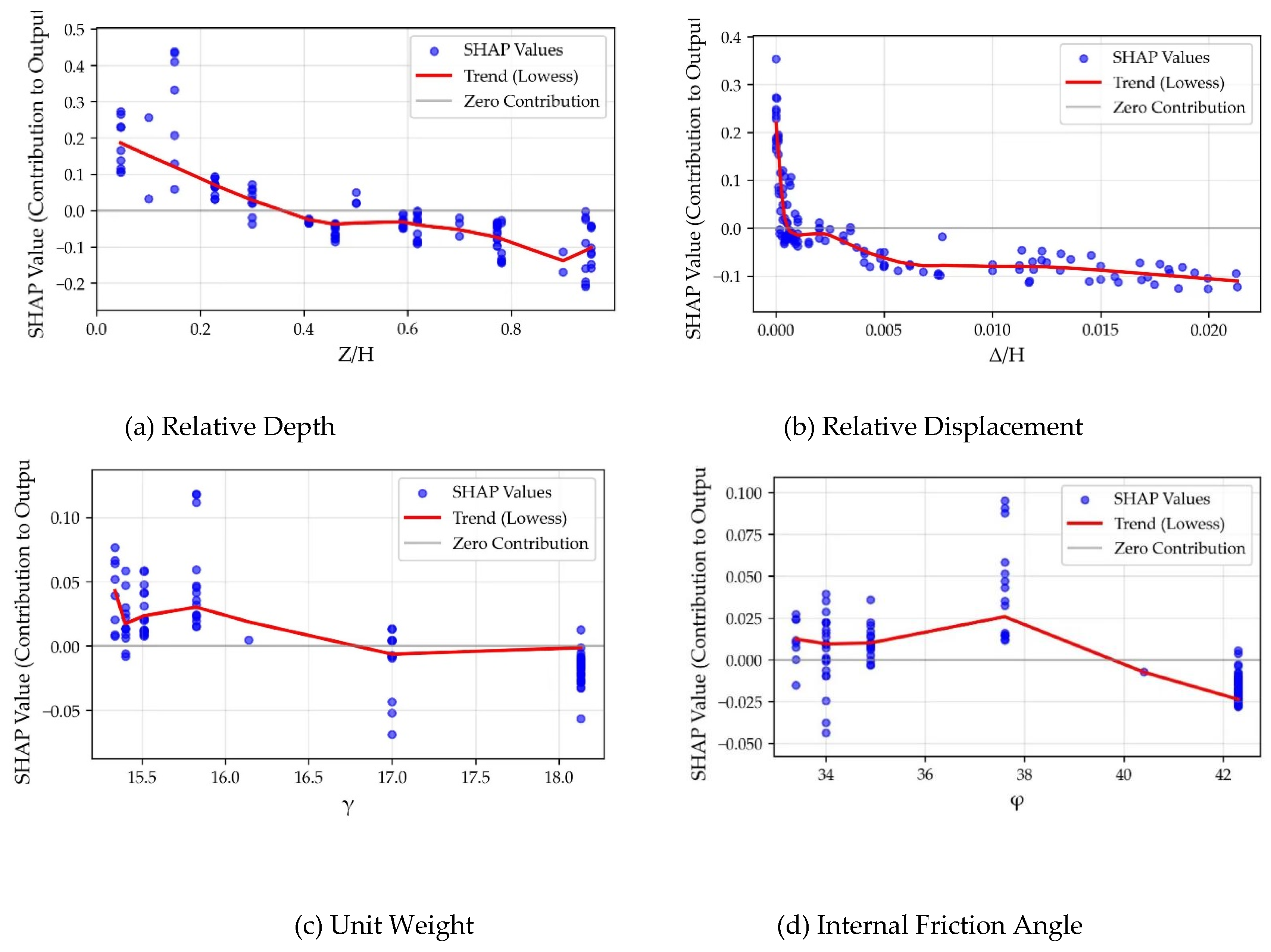
To examine more clearly how the earth pressure coefficient varies with different input features, SHAP dependence plots for individual features are presented in Figure 7. In these plots, the horizontal axis represents the value of the input feature, and the vertical axis represents the corresponding SHAP value, which quantifies the feature's contribution to the model output for each prediction. Each blue point corresponds to a sample from the test set, and its vertical position indicates the SHAP value for that feature when all other features are fixed at their average values. The red line represents the smoothed dependence curve, illustrating the overall nonlinear trend of the feature's contribution as its value changes.

As shown in the scatter points of Figure 7(a), smaller Z/H values correspond to larger SHAP values, indicating that samples from shallower soil depths tend to increase the predicted earth pressure coefficient K. The vertical distribution of SHAP values for this feature primarily ranges between –0.2 and 0.4, which exceeds the variation intervals observed for other features and further confirms its dominant role in the model. This pattern aligns with the variation of earth pressure coefficients along the wall height reported in experimental studies such as those by Fang et al. [16] and Singh et al. [28]. These findings differ from classical Rankine and Coulomb earth pressure theories, demonstrating that the present model successfully captures the variation of the earth pressure coefficient along the wall height. Such insight offers valuable guidance for retaining wall design, particularly regarding the structural strength requirements along different sections of the wall.

Figure 7(b) shows that in the initial stage (0 < Δ/H ≤ 0.001), SHAP values decrease sharply with increasing displacement. Beyond Δ/H > 0.001, the decrease becomes more gradual. This pattern suggests that earth pressure drops rapidly during the initial phase of wall movement and then stabilizes as displacement continues. The SHAP scatter points closely follow the dependence curve with a narrow distribution, indicating that Δ/H acts as a relatively independent feature with minimal interaction effects from other variables. From the perspective of local feature analysis, Figure 7(b) visually illustrates the smooth, continuous reduction of the earth pressure coefficient from the at-rest condition toward the active state.

Figure 7(c) shows that K decreases as γ increases generally. This trend can be explained physically: soils with lower density generally exhibit smaller internal friction angles and lower shear strength, leading to higher earth pressure coefficients. Fang et al. [16] also noted that the soil arching effect becomes more pronounced with increasing soil density. In engineering practice, compacting the backfill behind retaining walls can enhance shear strength and consequently reduce the earth pressure coefficient, which is crucial for ensuring structural safety.

As shown in Figure 7(d), the dependence curve reveals a more nuanced, nonlinear relationship: within the range of approximately 31.5° to 38°, the earth pressure coefficient tends to increase slightly with φ, beyond which it exhibits a decreasing trend as φ further increases. This demonstrates a complex, non-monotonic interaction between φ and K under the coupled influence of other factors captured by the model. In engineering practice, employing sandy backfill with a higher internal friction angle can generally be an effective measure to reduce the earth pressure coefficient and consequently lower the lateral pressure on the retaining structure.

4.4. Analysis of Feature Interactions in Earth Pressure

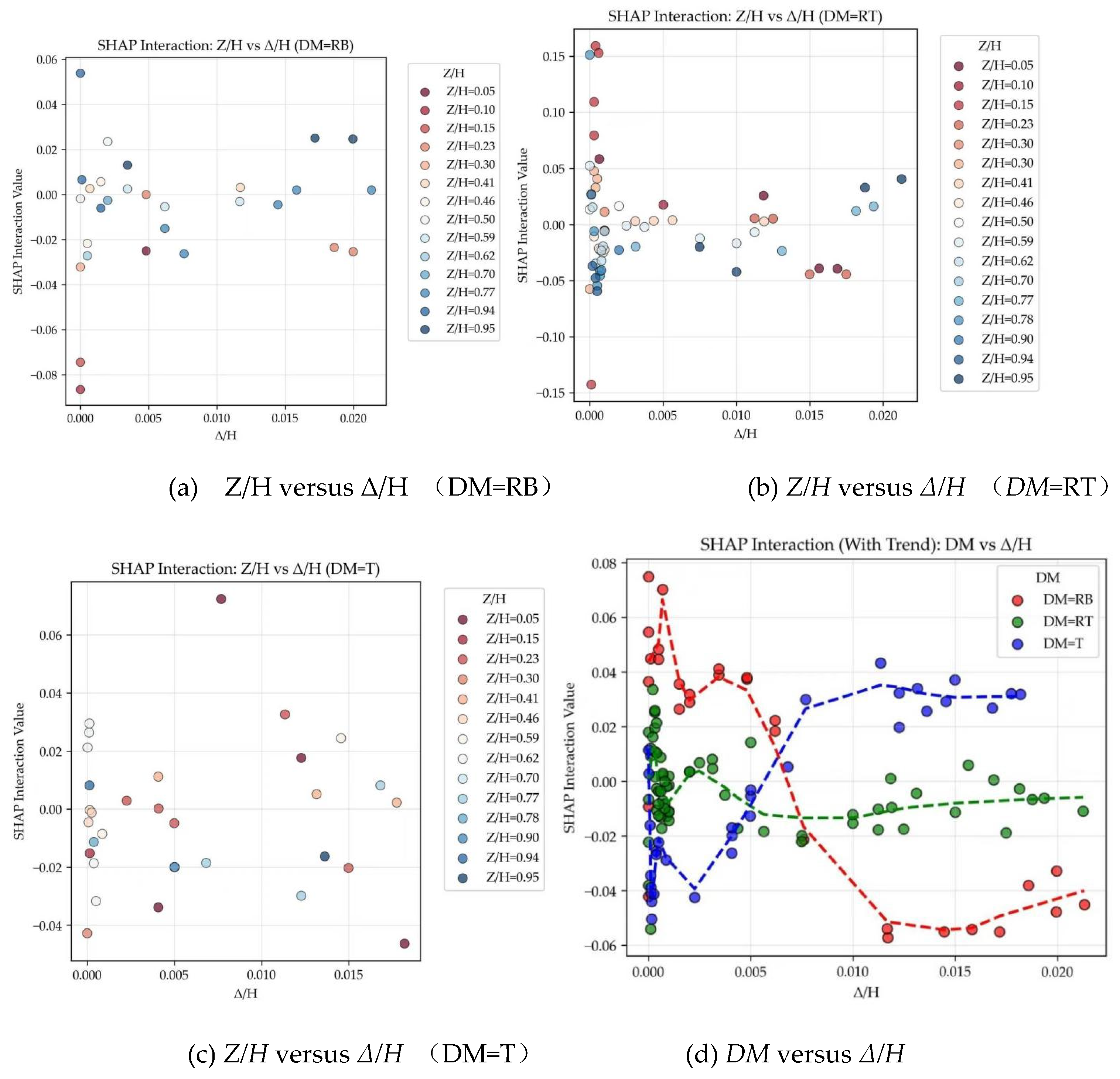
To further elucidate the nonlinear mechanisms of stress redistribution within the backfill, SHAP dependence interaction plots are constructed to examine the interactions between relative displacement (Δ/H) and relative depth (Z/H), as well as between Δ/H and displacement mode (DM), as shown in Figure 8. In these plots, the horizontal axis represents the primary feature (Δ/H), and the vertical axis shows the SHAP values for the combined effect of the primary and interaction features. The interactive feature levels are distinguished by different colors in the scatter points.

It is noteworthy that although the lateral earth pressure under at-rest conditions is generally considered to distribute linearly with depth [17,20], the actual measured earth pressure coefficients in model tests often exhibit fluctuations along the wall height. These variations can be attributed to factors such as soil overconsolidation, non-uniform compaction, and spatial variability of the wall-soil interface friction angle [18]. Consequently, the wider scatter band observed in Figure 8 at Δ/H = 0 does not necessarily indicate stronger interaction effects under static conditions. Instead, the analytical focus should be directed toward the evolving trend in the scatter distribution as Δ/H increases.

4.4.1. Interaction between Relative Displacement (Δ/H) and Relative Depth (Z/H)

Figures 8(a) to 8(c) present the SHAP dependence interaction plots for relative displacement (Δ/H) versus relative depth (Z/H) under the rotation-about-the-base (RB), rotation-about-the-top (RT), and translation (T) modes, respectively. These plots provide an in-depth visualization of the spatial non-uniformity in the backfill stress state, revealing how the sensitivity of the earth pressure coefficient to wall displacement varies with depth—a variation that is itself dependent on the wall movement mode.

Figure 8(a) (RB mode) shows that as Δ/H increases, the SHAP values rapidly converge toward the baseline (zero). Scatter points corresponding to shallow depths (low Z/H) are predominantly clustered in the negative SHAP region, whereas those for greater depths (high Z/H) appear in the positive region. Furthermore, shallow points exhibit a greater deviation from the baseline compared to deep points. This pattern occurs because, in the RB mode, the shallow soil zone undergoes the largest displacement, leading to the most complete stress release. As Δ/H increases, the interactive contribution to the earth pressure coefficient reaches its maximum (strongly negative SHAP values) in the shallow zone, indicating a rapid convergence toward active pressure conditions. In contrast, the displacement at the wall base is zero, imposing kinematic constraints on the deep soil layer. Consequently, the corrective influence of Δ/H on the earth pressure in deep layers weakens, with the interaction contribution approaching zero or even slightly positive values. This reflects the delayed release of the stress state in deep soil and suggests an upward shift in the point of application of the resultant lateral force.

As shown in Figure 8(b) (RT mode), with increasing Δ/H, the SHAP values again converge toward the baseline. In this mode, scatter points in the shallow zone (low Z/H) are predominantly distributed in the positive SHAP region, whereas those in the deep zone (high Z/H) fall mainly within the negative region. This distribution occurs because, under rotation about the top (RT), the soil near the restrained wall top experiences a stress concentration (enhanced soil arching effect). Consequently, even as Δ/H increases, the interactive contribution in the shallow zone initially remains positive before eventually transitioning to negative values—a shift that may correspond to the progressive failure of the soil arch. In contrast, the deep zone remains within the negative SHAP region throughout the displacement process, indicating a sustained reduction in earth pressure in the soil beneath the arch as displacement increases. This observation aligns with the findings of Zhang et al. [29], who noted that the arching effect is most pronounced in the RT displacement mode.

Figure 8(c) (Translation mode, T) shows that the scatter points exhibit no pronounced stratified trend with increasing Δ/H. This pattern occurs because, under the translational mode, wall displacement is uniform along the depth. The interaction between Δ/H and Z/H is relatively straightforward, as the variation in earth pressure is governed primarily by the linear increase in overburden stress with depth and the wall-soil friction, rather than by a displacement gradient. Consequently, the influence of Δ/H on earth pressure is similar across all depths, which explains the absence of distinct clustering between shallow and deep points in the interaction plot. Minor variations among some scatter points in Figure 8(c) may be attributed to slight changes in soil stiffness or density with depth.

The SHAP interaction analysis between Δ/H and Z/H confirms that the model's learned relationships align with fundamental principles of soil mechanics, particularly regarding the spatial non-uniformity of earth pressure. In the rotation-about-the-base (RB) mode, the strongly negative interaction in shallow regions highlights the rapid initial stress relaxation near the wall crown, which diminishes toward the constrained base. In contrast, the rotation-about-the-top (RT) mode reveals a more complex, nonlinear interaction where the effect of Δ/H is attenuated near the top (Z/H ≈ 0). This pattern reflects the model's incorporation of the soil arching mechanism, which locally counteracts the pressure reduction typically induced by displacement. These insights are consistent with the experimental observations of Rui et al. [18] and Fang et al. [16]. Therefore, the interaction plots provide compelling evidence that the machine learning model has successfully captured and internalized key soil-structure interaction mechanisms dependent on wall kinematics.

4.4.2. Interaction between Relative Displacement (Δ/H) and Displacement Mode (DM)

As illustrated in Figure 8(d), during the small displacement stage (Δ/H < 0.005), the rotation-about-the-base (RB) mode exhibits the highest and positive SHAP interaction value. In this stage, corresponding to the initial formation of the failure surface, significant outward displacement occurs primarily at the wall crown. The upper soil zone enters a state of stress relaxation while the lower zone retains higher lateral stress (close to the at-rest condition), resulting in elevated SHAP values. As displacement increases, the SHAP values for the RB mode decrease sharply from positive to strongly negative. This trend characterizes the progressive development of the failure surface from the top downward. Once the failure plane fully propagates through the soil mass, the RB mode facilitates the most complete spatial stress relaxation, causing the earth pressure coefficient to drop rapidly toward the active limit state.

In contrast, the trend for the translational (T) mode is markedly different: it contributes negative SHAP values at low displacements and shifts to a significant positive contribution as displacement increases. Under translational movement, the soil must attain a shear failure strain simultaneously at all depths to reach a uniform active state. Lacking the geometric advantage of localized, sequential stress relief seen in the RB mode, the T mode requires larger overall displacements to mobilize comparable pressure reduction. Consequently, at similar displacement magnitudes, the earth pressure coefficient for the T mode consistently exceeds that for rotational modes, reflecting the soil’s structural integrity and the lag in stress release during widespread displacement.

The rotation-about-the-top (RT) mode exhibits the most stable SHAP interaction behavior across the entire displacement range, fluctuating near zero. This mode is typical in top-constrained structures such as bridge abutments. The restraint at the wall top forces the failure surface to develop upward from the base, generating a pronounced soil arching effect that transfers stress from the high-displacement lower zone to the constrained upper zone. This internal stress redistribution mechanism physically offsets the pressure reduction expected from displacement alone, resulting in low sensitivity within the prediction model and demonstrating strong nonlinear robustness.

The analysis reveals that the SHAP interaction curves for the three modes intersect near Δ/H ≈ 0.006. This intersection point carries important mechanical implications: before this threshold, the spatial distribution of displacement (i.e., the mode) dominates the stress response; beyond it, the magnitude of displacement becomes the primary driver pushing the soil system toward a generalized active equilibrium state. This finding suggests that traditional Rankine or Coulomb theories—typically based on translational assumptions—may significantly overestimate earth pressure under RB conditions. Conversely, under RT conditions, these theories may overlook local stress concentrations due to arching, leading to potential inaccuracies in assessing the safety and economy of engineering designs.

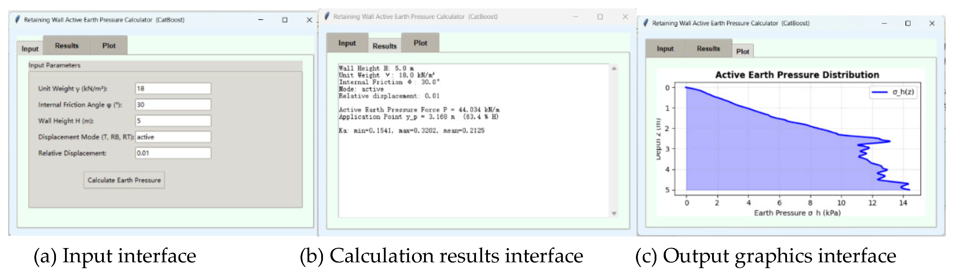
5. Development and Validation of the GUI Tool

5.1. GUI Tool Design

A graphical user interface (GUI) program is developed to calculate the lateral earth pressure behind retaining walls with sandy backfills, based on the model established with the CatBoost algorithm using default hyperparameters. The program is applicable for both limit state and non-limit state analyses. Users can input fundamental parameters, including the internal friction angle (φ), unit weight (γ), wall height (H), displacement mode (DM), and relative displacement of the wall (Δ/H). The program then invokes the trained CatBoost model to compute the distribution of the earth pressure coefficients along the wall depth. Utilizing numerical integration, it calculates both the magnitude and the application point of the resultant earth pressure force and graphically displays the pressure distribution along the wall depth. The GUI is designed with an intuitive layout, ease of operation, and strong practical applicability for engineering use. The interface of the GUI program is shown in Figure 9.

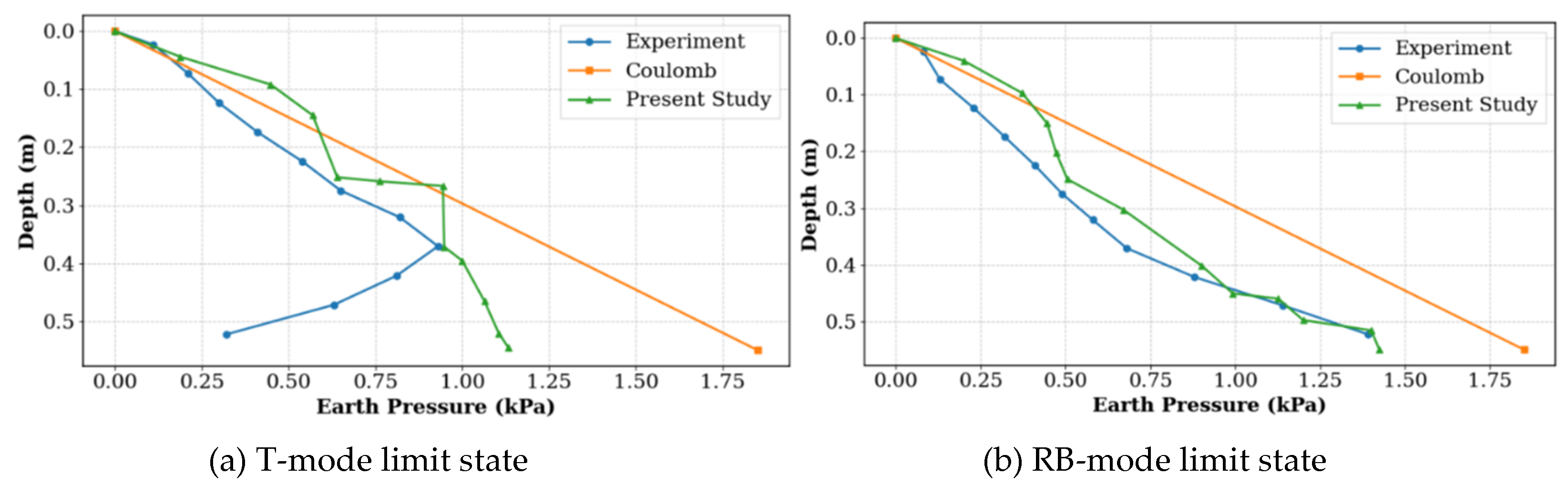
5.2. Validation with Independent Test Data

To validate the accuracy of the developed GUI tool, two independent test cases from the model experiments by Rui et al. [18]—which reached the active limit state under translation (T) and rotation-about-the-base (RB) modes—are selected. Predictions from the GUI tool are compared with those from Coulomb’s theoretical formula. These specific samples are not included in the original model training dataset. The soil parameters are: unit weight γ = 18.13 kN/m³, internal friction angle φ = 42.3°, and wall height H = 0.55 m. The normalized displacements at the active limit state Δ/H = 0.0027 for the T mode and Δ/H = 0.00896 for the RB mode. For the Coulomb theoretical calculation, the wall–soil interface friction angle is taken as 0.5φ.

Comparison of the earth pressure distributions obtained from the experimental measurements, Coulomb’s theory, and the present GUI tool are shown in Figure 10. Figure 10(a) corresponds to the T mode at the active limit state, and Figure 10(b) to the RB mode. In both subfigures, the horizontal axis represents the lateral earth pressure, and the vertical axis denotes the depth. The blue line indicates the experimental results, the orange line represents the Coulomb theoretical distribution, and the green line shows the prediction from the GUI tool.

As clearly illustrated in Figure 10, the predictions from the GUI tool developed in this study align more closely with the experimental measurements than those from Coulomb’s theory, demonstrating higher accuracy and practical engineering applicability, particularly under nonlinear, displacement-coupled conditions.

6. Conclusions and Prospects

This study addresses the limitations of classical earth pressure theory and current challenges regarding the interpretability of ML models. One of the objectives of this study is to establish a ML database for predicting earth pressure for rigid retaining walls with sandy backfill under various displacement modes and magnitudes. This database encompasses both limit and non-limit states, and it is developed using relevant model test data from the literature. A “key feature refinement strategy based on collinearity analysis” is proposed and validated. This proposal identifies a set of only five fundamental physical parameters, which is optimal in the sense that it achieves the best possible balance between model accuracy and interpretability. The model utilizes the CatBoost/SHAP framework to effectively elucidate the mechanisms governing earth pressure during wall displacement, thereby revealing complex nonlinear relationships and interactions among the influencing factors. Finally, the development of a user-friendly GUI program has been accomplished, thereby establishing a connection between theoretical outcomes and practical engineering applications. The main conclusions are as follows:

1) A streamlined feature set for predicting the earth pressure coefficient is constructed using a collinearity-driven strategy. This strategy is a systematic approach for comparing correlation coefficients and the variance inflation factor (VIF). It is also an assessment of the model's accuracy and interpretability. This process confirms that the interpretability is of comparable importance to predictive accuracy in contemporary ML applications for geotechnical engineering.

2) For rigid retaining walls in the case of an active state, the prevailing factors influencing the earth pressure coefficient are identified as the relative depth (Z/H) and relative displacement (Δ/H). Subsequent factors include displacement mode, soil unit weight, and internal friction angle. The earth pressure coefficient behind retaining walls exhibits a distinct nonlinearity along the depth, in contrast to the predictions of classical Rankine and Coulomb theories.

3) A SHAP dependence analysis reveals a monotonic decrease in the earth pressure coefficient with increasing relative depth. During the transition from an at-rest condition to displacement, the coefficient experiences a precipitous drop before undergoing a more gradual decrease. While the influences of internal friction angle and unit weight demonstrate variability, the overall trend indicates a decline in the coefficient with increasing values of either parameter.

4) A detailed investigation into SHAP interaction analysis has yielded a comprehensive insight into the nonlinear mechanisms of stress redistribution behind the wall. Displacement modes (i.e., RB, RT, T) have been identified as the primary factors that regulate the spatial non-uniformity of earth pressure. A mechanical threshold is identified at a smaller displacement of Δ/H, the motion pattern dominates the pressure response; beyond this threshold, however, the displacement magnitude drives the system toward a generalized active equilibrium. The findings presented herein effectively visualize classical soil mechanics mechanisms, including top-down stress relaxation in the RB mode and soil arching in the RT mode. This provides kinematics-dependent evidence for a refined wall design.

5) Independent case studies have been conducted to validate the developed GUI program, and the results indicate that it provides more accurate predictions of backfill pressure than classical Rankine and Coulomb theories. These findings suggest a high degree of potential for the practical engineering applications of the program.

The present study investigates the earth pressure on rigid retaining walls under various displacement modes, thereby overcoming the limitations of classical Rankine and Coulomb theories in predicting the complex nonlinear and displacement-coupled behavior under non-limit states. The findings of this study contribute to the advancement of mechanistic understanding of earth pressure behind retaining walls. In addition, they provide a direct theoretical basis and a practical computational tool for the design of walls undergoing controlled, pattern-specific displacements in engineering practice. The developed GUI program, with its intuitive interface and reliable computational engine, effectively bridges the gap between research outcomes and practical applications.

Limitations and Outlook: The machine learning database employed in this study has been derived from published model test data. Due to the limited availability of literature with detailed experimental records, the current dataset remains constrained in both scope and sample diversity. In addition, it should be noted that model tests are inherently influenced by specific laboratory conditions and scale effects. This influence can lead to potential discrepancies with real-world field behavior. Consequently, the direct transferability of the model to actual engineering scenarios is limited. Consequently, subsequent endeavors should prioritize the expansion of the scale and diversity of the dataset. This objective should be pursued, in part, by incorporating more field monitoring and in-situ test data to enhance the model's generalization capability. Concurrently, systematic refinement of input feature selection (e.g., inclusion of the wall-soil interface friction angle) and optimization of data balance are necessary. The exploration of machine learning frameworks that are more interpretable will result in enhanced predictive accuracy and reliability. This, in turn, will promote the broader adoption of this methodology in engineering practice.

References

- Nguyen, T. An Exact Solution of Active Earth Pressure Based on a Statically Admissible Stress Field. Comput. Geotech. 2023, 153, 1-24. [CrossRef]
- Qian, J.; Zhou, C.; Li, W.; Gu, X.; Qin, Y.; Xie, L. Investigation on the Influencing Factors of K0 of Granular Materials Using Discrete Element Modelling. Appl. Sci. 2022, 12(6). [CrossRef]
- Ma, K.; Wang, L.; Long, L.; Peng, Y.; He, G. Discrete Element Analysis of Structural Characteristics of Stepped Reinforced Soil Retaining Wall. Geomatics. Nat. Hazards Risk, 2020, 11(1): 1447–1465. doi: 10.1080/19475705.2020.1797907.
- Yang, M.; Deng, B. Simplified Method for Calculating the Active Earth Pressure on Retaining Walls of Narrow Backfill Width Based on DEM Analysis. Adv. Civ. Eng. 2019. doi: 10. 1155/2019/1507825.
- Li, T.; Huo, J.; He, P.; Liu, X.; Fang, X. Comprehensive Review of Earth Pressures on Retaining Structure[J]. J. Guilin Univ. Technol. 2017, 37, 94-102. doi: 10.3969/j.issn.1674-9057.2017.01.013.
- Patsevich, A.; El Shamy, U. Discrete-element Method Study of the Seismic Response of Gravity Retaining Walls. Int. J. Geomech. 2020, 20(11). doi: 10.1061/(asce)gm.19435622.0001837.
- Wang, Y.; Mora, P.; Liang, Y. Calibration of Discrete Element Modeling: Scaling Laws and Dimensionless Analysis. Particuology 2022, 62: 55–62. doi: 10.1016/j.partic.2021.03.020.
- Li, Z.; Yang, X. Three-dimensional Active Earth Pressure for Retaining Structures in Soils Subjected to Steady Unsaturated Seepage Effects. Acta Geotech. 2019, 15(7): 2017-2029. [CrossRef]
- Peng S.; Li X.; Fan L. Meso-scale of Soil Arching for Rigid Retaining Wall Active Failure. J. Cent. South Univ. (Sci. Technol.) 2011, 42(4): 1099-1104.
- Handy R. L. The Arch in Soil Arching. J. Geotech. Eng. 1985, 111(3): 302—318. [CrossRef]
- Liu Y.; Yu P. Analysis of Soil Arch and Active Earth Pressure on Translating Rigid Retaining Walls. Rock Soil Mech. 2019, 40(2): 506-528. [CrossRef]
- Lu W.; Wang X.; Yang P.; Cui L.; Ren Y.; Jin K. Analysis of Soil Arching Effect of Active Earth Pressure on Rigid Retaining Wall with Translation Mode. J. Lanzhou Univ. Technol. 2017, 43(1): 132-136.
- Zhou Y.; Yang D. Calculation and Analysis of Active Earth Pressure on Retaining Walls Considering Soil Arching Effects. J. Hohai Univ. (Nat. Sci.) 2016, 44(2): 149-154. [CrossRef]
- Wang M.; Li J. New Method for Active Earth Pressure of Rigid Retaining Walls Considering Arching Effect. Chin. J. Geotech. Eng. 2013, 35(5): 865-870. [CrossRef]
- Chang, M. Lateral earth pressures behind rotating walls. Can. Geotech. J. 1997, 34: 498–509. [CrossRef]
- Fang, Y.; lshibashi, I. Static Earth Pressure with Various Wall Movements. J. Geotech. Eng. 1986, 112 (3): 317-333. [CrossRef]
- Zhou, Y.; Ren, M. An Experimental Study on Active Earth Pressure behind Rigid Retaining Wall. Chin. J. Geotech. Eng. 1990, 12 (2): 19-26. [CrossRef]
- Rui, R.; Jiang, W.; Xu, Y.; Xia, R.; Edo, E. E.; Ding, R. Experimental Study of the Earth Pressure on a Rigid Retaining Wall for Various Patterns of Movements. Chin. J. Rock Mech. Eng. 2023, 42 (6): 1534-1545. doi: 10.13722/j.cnki.jrme.2022.0808.
- Shi, W. Model Test and Analytical Research on the Active Earth Pressure Acting on a Rigid Retaining Wall. Master, Chang’an University, Xi’an, China, April 2019.
- Gong, H. Calculation Method and Experimental Verification of Unsaturated Soil Pressure Considering Displacement Effect. Master, Hunan University, Changsha, China, April 2023.
- Yang, X.; Chen, H. Seismic Active Earth Pressure of Unsaturated Soils with a Crack Using Pseudo-dynamic Approach. Comput. Geotech. 2020, 125: 103684.1-103684.12. [CrossRef]
- Patel, S.; Deb, K. Study of Active Earth Pressure Behind a Vertical Retaining Wall Subjected to Rotation about the Base. Int. J. Geomech. 2020, 20 (4). [CrossRef]
- Qian, Z.-H.; Zou, J.-F.; Tian, J.; Pan, Q. J. Estimations of Active and Passive Earth Thrusts of Non-homogeneous Frictional Soils Using a Discretisation Technique. Comput. Geotech. 119, 103366. [CrossRef]
- Nguyen, T. Passive Earth Pressures with Sloping Backfill Based on a Statically Admissible Stress Field. Comput. Geotech. 2022,149, 104857. [CrossRef]
- Zhang, F.; Yin, M.; Sun, F.; et al. Non-limit Active Earth Pressure Under Different Retaining Wall Displacement Modes Based on Discrete Element Simulation. Sci. Technol. Eng. 2024, 24(11): 4658-4668. [CrossRef]
- Shi, F.; Lu, K.; Yin, Z. Determination of Three-dimensional Passive Slip Surface of Rigid Retaining Walls in Translational Failure Mode and Calculation of Earth Pressures. Rock Soil Mech. 2021, 42(3): 735-745. [CrossRef]
- Wan, L.; Zhang, X.; Wang, Y.; Xu, L.; Xu, C. Study on Active Failure and earth Pressure of Cohesionless Soil with Limited Width behind Retaining Wall. J. Civ. Environ. Eng. 2019, 41 (3): 19-26. [CrossRef]
- Singh, P.; Chakraborty, T.; Mahajan, P. Discrete Element Study of Stresses and Deformation on Gravity Retaining Wall under Static Loading. Granu. Matter 2024, 26 (48):1-14. [CrossRef]
- Zhang, H.; Xu, C.; He, Z.; Huang, Z.; He, X. Study of Active Earth Pressure of Finite Soils under Different Retaining Wall Movement Modes Based on Discrete Element Method. Rock Soil Mech. 2022, 43(1): 257-267. [CrossRef]
- Chen, H.; Chen, F.; Chen, C.; Lai, D. Failure Mechanism and Active Earth Pressure of Narrow Backfills behind Retaining Structures Rotating about the Base. Int. J. Geomech. 2024, 24(5):04024068-1-13. [CrossRef]
- Xiong, C.; Tang, W.; Xing, Z.; Zheng, J.; Liu, Y.; Jiang, X.; Li, X.; Chen, Y. Active Earth Pressure of Narrow Cohesionless Backfill on Balance Weight Retaining Walls Rotating about the Bottom. Structures 2024, 67 (2024):1-12. [CrossRef]
- Hang, L.; H.; Dang, F.; Wang, X.; Ding, J.; Gao, J. Calculation and Analysis of Earth Pressure under Limited Displacement Considering Influences of Internal Friction Angle. Chin. J. Geotech. Eng. 2021, 43 (1):81-86.
- Shin, J.; Han, H. Analysis of the Impact on Prediction Models Based on Data Scaling and Data Splitting Methods - For Retaining Walls with Ground Anchors Installed. J. Eng. Geol. 2023, 33 (4): 639-655. [CrossRef]
- Zhang, W. G.; Gou, A. T. C. Multivariate Adaptive Regression Splines for Analysis of Geotechnical Engineering Systems. Comput. Geotech. 2013, 48: 82-95. [CrossRef]
- Mishra, P.; Samui, P.; Mahmoudi, E. Probabilistic Design of Retaining Wall Using Machine Learning Methods. Appl. Sci. 2021, 11(12). [CrossRef]
- Aydın, Y.; Bekdaş, G.; Nigdeli, S. Dimensioning of the Retaining Wall Using Linear Regression, Ridge Regression and Lasso Regresion. In Proceedings of the conference on New Technologies, Development and Application (NT-2025), Sarajevo, Bosnia and Herzego, June 2025. doi: org/10.1007/978-3-031-95200-5_53.
- Bekdaş, G.; Cakiroglu, C.; Kim, S.; Geem, Z. Optimal Dimensioning of Retaining Walls Using Explainable Ensemble Learning Algorithms. Materials 2022, 15, (14). [CrossRef]
- Lundberg, S.; Lee, S. A Unified Approach to Interpreting Model Predictions. Neural Information Processing Systems Conference, Long Beach, CA, USA, 2017, 30. [CrossRef]
- Minoru, M.; Satoru, K.; Hiderki, Y. Experimental Study on Earth Pressure of Retaining Wall by Field Tests. Japanese Society of Soil Mechanics and Foundation Engineering 1978, 18 (3):27-41. [CrossRef]
- Ke, G.; Meng, Q.; Finley, T.; Wang, T.; Chen, W.; Ma, W.; Ye, Q.; Liu, T.-Y. LightGBM: A highly efficient gradient boosting decision tree. Adv. Neural Inf. Process. Syst. 2017, 30, 3146–3154.
- Uddin, M.N.; Ye, J.; Deng, B.; Li, L.; Yu, K. Interpretable Machine Learning for Predicting the Strength of 3D Printed Fiber Reinforced Concrete (3DP-FRC). J. Build. Eng. 2023, 72, 106648. [CrossRef]
- Rahman, J.; Ahmed, K.S.; Khan, N.I.; Islam, K.; Mangalathu, S. Data-Driven Shear Strength Prediction of Steel Fiber Reinforced Concrete Beams Using Machine Learning Approach. Eng. Struct. 2021, 233, 111743. [CrossRef]
- Song, Y.; Wang, F.; Yang, W.; Liang, R.; Zhan, D.; Xiang, M.; Yang, X.; Xu, R.; Lu, M. High-Performance Prediction of Soil Organic Carbon Using Automatic Hyperparameter Optimization Method in the Yellow River Delta of China. Comput. Electron. Agric. 2025, 236, 110490. [CrossRef]
- Boser, B.E.; Guyon, I.M.; Vapnik, V.N. A Training Algorithm for Optimal Margin Classifiers. In Proceedings of the Fifth Annual Workshop on Computational Learning Theory; ACM: Pittsburgh, PA, USA, 1992; pp. 144–152. [CrossRef]
- Solhmirzaei, R.; Salehi, H.; Kodur, V. Predicting flexural capacity of ultrahigh-performance concrete beams: Machine learning based approach. J. Struct. Eng. 2022, 148, 04022031. [CrossRef]
- Yang, Y.; Yang, Y. Hybrid Prediction Method for Wind Speed Combining Ensemble Empirical Mode Decomposition and Bayesian Ridge Regression. IEEE Access 2020, 8, 71206–71218. [CrossRef]
- Ye, M.; Li, L.; Yoo, D.-Y.; Li, H.; Zhou, C.; Shao, X. Prediction of Shear Strength in UHPC Beams Using Machine Learning-Based Models and SHAP Interpretation. Constr. Build. Mater. 2023, 408, 133752. [CrossRef]
- Zhang, Z.; Zeng, T.; Zeng, Y.; Zhu, P. Explainable Prediction of UHPC Tensile Strength Using Machine Learning with Engineered Features and Multi- Algorithm Comparative Evaluation. Buildings 2025, 15, 3217. [CrossRef]
- Ke, L.; Qiu, M.; Chen, Z.; Zhou, J.; Feng, Z.; Long, J. An Interpretable Machine Learning Model for Predicting of CFRP-Steel Epoxybonded Interface. Compos. Struct. 2023, 326, 117639. doi: 10.1016/j.compstruct.2023.117639.
- Zhang, Z.; Zhou, X.; Zhu, P.; Li, Z.; Wang, Y. Prediction of Flexural Ultimate Capacity for Reinforced UHPC Beams Using Ensemble Learning and SHAP Method. Buildings 2025, 15, 969. [CrossRef]
- Lundberg, S.; Lee, S.-I. A Unified Approach to Interpreting Model Predictions. In Proceedings of the conference on Neural Information Proceedings Systems (NIPS 2017), Long Beach, CA, USA, 25 November 2017; pp.4765-4774.
- Arslan, Y.; Lebichot, B.; Kevin Allix, K.; Veiber, L.; Lefebvre, C; Boytsov, A; Goujon, A.; Bissyandé, T.; Klein, J. Towards Refined Classifications driven by SHAP Explanations. International Cross-Domain Conference for Machine Learning and Knowledge Extraction; IFIP, Vienna, Austria, 2022, 4: 68-81. [CrossRef]
- Antwarg, L.; Shapira, B.; Rokach, L. Explaining Anomalies Detected by Autoencoders Using Shapley Additive Explanations. Expert Syst. Appl. 2021, 186. [CrossRef]
- Gramegna, A.; Giudici, P. SHAP and LIME: An Evaluation of Discriminative Power in Credit Risk. Front. Artif. Intell. 2021, 4. [CrossRef]
- Lu k.; Zhu D.;‚Yang Y. Calculation Method of Active Earth Pressure Under Non-limit State Considering Soil Arching Effects. China J. Highw. Transp. 2010, 23 (1): 19-25.