1. Introduction
Sour around bridge piers and abutments is one of the most important structural safety problems in the field of hydraulic engineering. The erosion of the bed material around the bridge piers and abutments can lead to the weakening of the bridge structure and even its collapse over time.
The estimation of scour depth has been traditionally conducted using empirical equations and physical modeling approaches. Early studies, such as those by Melville and Coleman, established fundamental empirical relationships for predicting scour depth based on hydraulic parameters [
1]. Similarly, HEC-18 guidelines by the Federal Highway Administration have been widely used in engineering practice. However, these methods often lack adaptability to varying site conditions and exhibit limitations in predictive accuracy [
2].
Recent advancements in artificial intelligence and machine learning have provided more sophisticated tools for scour depth prediction. Studies by Lee et al. and Azamathulla et al. demonstrated the effectiveness of machine learning models such as Support Vector Machines (SVM) and Artificial Neural Networks (ANN) in capturing complex nonlinear relationships between hydraulic variables and scour depth [
3,
4]. Additionally, ensemble learning techniques like Random Forest and XGBoost have shown promise in improving prediction accuracy and generalization capabilities [
5].
Several recent studies published in MDPI’s Water journal have further contributed to this field. For instance, a study by Hamidifar et al. highlighted that hybrid models combining empirical equations and machine learning algorithms provide more reliable scour depth predictions [
6]. Another study by Khan et al., used AI techniques to estimate scour depth with higher accuracy compared to traditional approaches. These findings emphasize the growing role of AI-driven models in hydraulic engineering [
7].
So, the estimation of the equilibrium scour depth (Dse) accurately is important for the safety and long-life of bridges at clear-water flow conditions. There are many studies for estimating equilibrium scour depth, like empirical equations and physical modeling studies for clear water conditions. However, these methods have limited generalization capabilities as they depend on specific field conditions, and they are not based on a large dataset.
In recent years, advances in artificial intelligence and machine learning techniques have provided the opportunity to model complex hydraulic processes accurately. In particular, machine learning-based approaches can capture nonlinear relationships between variables by learning from large datasets and producing more reliable estimates. In this study, various machine learning models such as Multiple Linear Regression (MLR), Support Vector Regression (SVR), Decision Tree Regressor (DTR), Random Forest Regressor (RFR), XGBoost (Extreme Gradient Boosting) and Artificial Neural Networks (ANN) will be used to estimate the scour depth in the equilibrium condition around the bridge side piers.
In this study, equilibrium scour depth (Dse) around bridge abutments was estimated by using the most effective hydraulic and sedimentological variables of flow depth (Y), pier length (L), channel width (B), flow velocity (V), and average grain diameter (D50). The performance of the models was evaluated with metrics such as Mean Square Error (MSE), Root Mean Square Error (RMSE), and Coefficient of Determination (R²), and the results will be supported with graphics.
At the end of the study, the effectiveness of machine learning models in scour depth was estimated, and the results of the machine learning applications and experimental measurements were compared. It was seen that the observed and experimentally measured data were almost 99% similar to each other. As a result, it was shown that data-driven estimation methods could be preferred and used safely in engineering applications, as opposed to previously used methods. Ultimately, this study seeks to demonstrate that AI-driven methods can provide more reliable and scalable solutions for scour depth estimation, contributing to safer and more resilient bridge infrastructure.
2. Materials and Methods
2.1. Local Scour
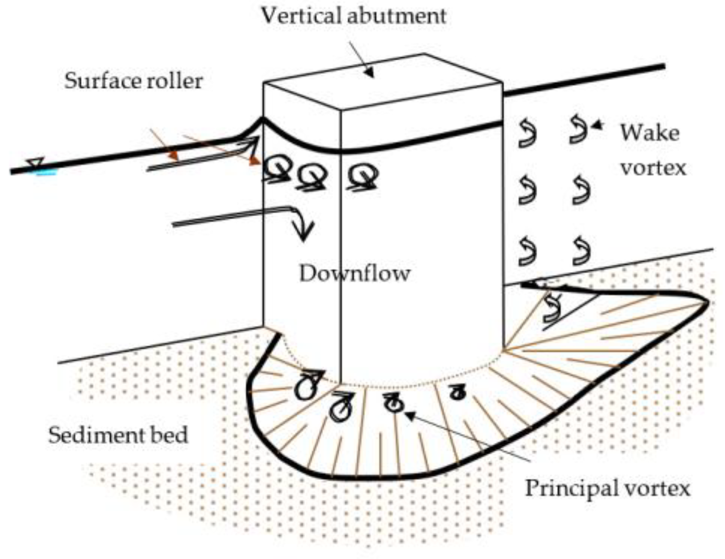
The basic mechanism causing local scour at bridge abutments is the formation of vortices at their base in
Figure 1 [
8]. The vortex moves bed material from the base of the abutment. If the outgoing rate of sediment transport rate is higher than the coming rate of sediment transport, the scour hole occurs. On the other hand, there are vertical vortices downstream of the structure called wake vortices. The force of wake vortices decreases rapidly while the distance downstream of the structure increases. Generally, the depths of local scour are much larger than general or contraction scour depths, often by a factor of ten [
2].
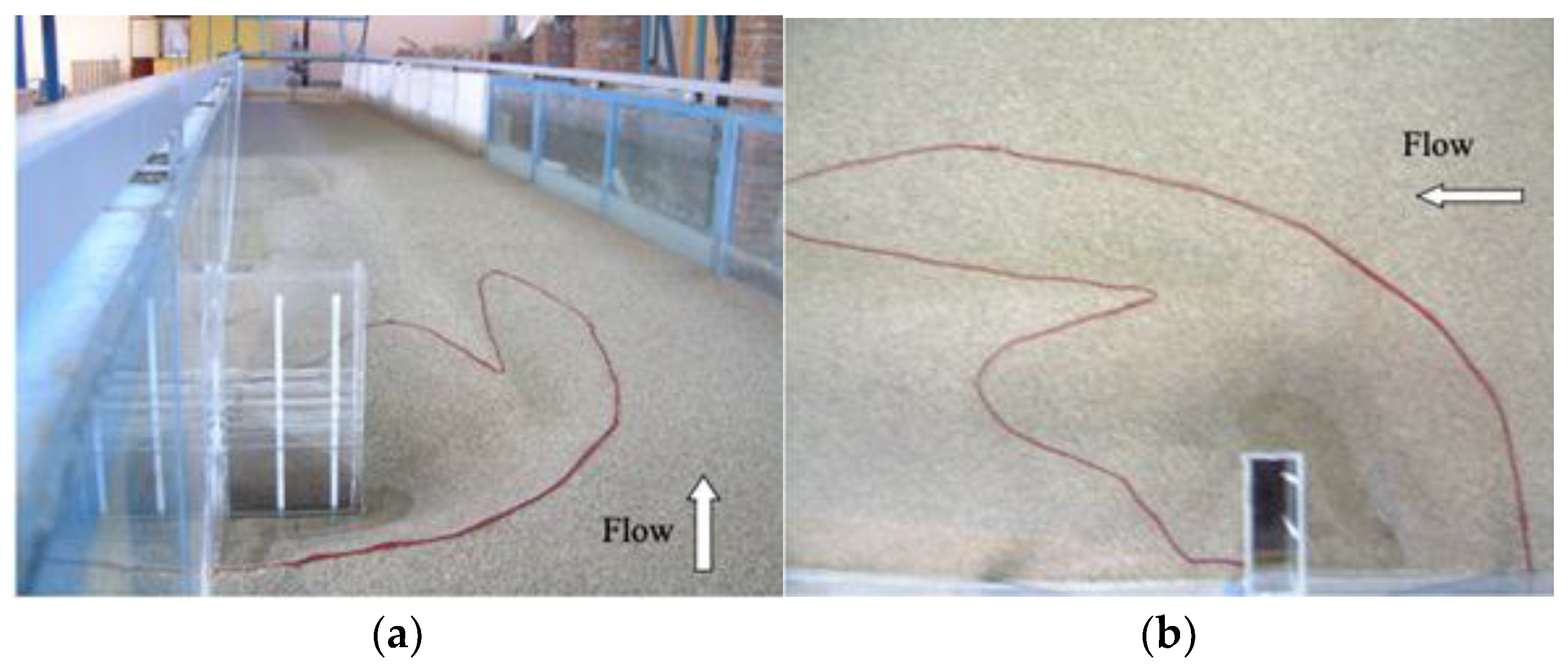
To show the local scour formation around bridge abutments visually, there is an experimental test studied in the Technical Research and Quality Control Laboratory of General Directorate of State Hydraulic Works for this study.
Figure 2 shows the formation of abutment scour obtained in the laboratory belonging to the experimental conditions of
B=150 cm,
L=25cm,
V=0.38 m/s,
D50=1.48 mm, and
Dse was measured as 10,2 cm.
The scour hole formation obtained by the experimental study is shown in
Figure 2.
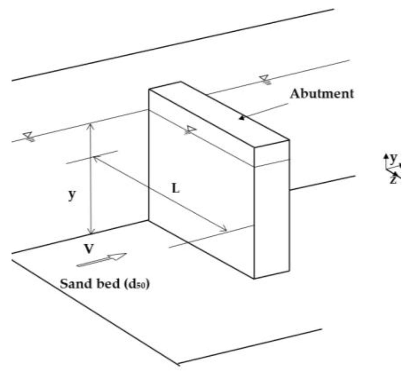
2.2. Parameters Affecting Scour Around Bridge Abutments
Factors that affect the magnitude of local scour depth at abutments are given in
Figure 3 [
8]. Their definitions are given below.
Flow velocity
Flow depth: An increase in flow depth can increase scour depth by a factor of 1.1 to 2.15, depending on the abutment shape [
2].
Abutment Length: Scour depth increases by increasing abutment length.
Bed material size and gradations: Bed material characteristics like gradation and cohesion can affect local scour.
Abutment Shape: As the streamlining shape of the butters reduces the strength of the horseshoe vortex and decreases scour depths
2.3. Parameters Affecting Scour Around Bridge Structures
For clear water approach flow conditions, the equilibrium scour depth (Dse) at a support point is a function of the parameters given in Equation 1:
where, B=abutment width, V=mean approach flow velocity, S=slope of the channel, g=gravitational acceleration, ρs= sediment density, ρ=the fluid density, μ=dynamic viscosity of fluid, D50=median particle grain size, σg=(d84/d16)0.5=geometric standard deviation of sediment size distribution, d84=sediment size for which 84% of the sediment is finer, d16= sediment size for which 16% of the sediment is finer, and t=scouring time.
In terms of dimensionless parameters
Dse can be described as Equation 2;
If the bed slope, duration of the experiment, the viscous effects are ignored one can simplify as Equation 3:
where the equilibrium scour depth is normalized with flow depth.
2.4. Dataset
This study envisages the evaluation and prediction of the results with various machine learning methods: Multiple Linear Regression, Support Vector Regression (SVR), Decision Tree Regressor, Random Forest Regressor, XGBoost, and Artificial Neural Networks (ANN). The dataset used in the study contains 150 data records, 5 features: Y (flow depth), L (abutment length), B (channel width), V (flow velocity), and D50 (average grain size), and 1 class (Dse (equilibrium scour depth)). The details of the dataset features are shown in
Table 1.
2.5. Multiple Linear Regression
Multiple Linear Regression (MLR) is a statistical method used to model the linear relationship between the dependent variable and more than one independent variable [
9]. Its main purpose is to estimate the dependent variable (
Dse - equilibrium scour depth) using certain independent variables (
Y, L, B, V, D50). The MLR model has the general formula stated in Equation 4.
where;
Dse is the desired equilibrium scour depth,
Y, L, B, V, D50 are independent variables (hydraulic and sedimentological parameters),
β0 is the constant term (intercept) of the model,
β1,
β2,...,
β5 are the coefficients of each independent variable (weights learned by the model),
ε is the error term (variability that cannot be explained by the independent variables).
Multiple linear regression is trained using the Ordinary Least Squares (OLS). The OLS method determines the model coefficients by minimizing the sum of the squares of the error term. The following metrics are generally used to evaluate the performance of the model [
9].
Mean Square Error (MSE) is the average of the squares of the differences between predicted and actual values. Root Mean Square Error (RMSE), the square root of the MSE, expresses the error size in the original measurement unit. The Coefficient of Determination (R2) shows how much the model explains the total variability in the dependent variable. It varies between 0 and 1; values close to 1 indicate that the model fits well.
The model is quite easy to interpret and apply. It offers the opportunity to analyze the effect of independent variables on the dependent variable separately. It can produce strong estimates, especially when it comes to linear relationships. If there is multicollinearity between independent variables, the reliability of the model may decrease. It cannot model nonlinear relationships well enough. Outliers and missing data can damage the model.
The MLR model will be compared with other machine learning models, and its accuracy in estimating the equilibrium scour depth will be evaluated in this study. The results will provide important information for comparing traditional linear methods with more advanced algorithms.
2.6. Support Vector Regression (SVR)
Support Vector Regression (SVR), unlike traditional regression methods, is a machine learning method that models the relationship between the dependent variable and the independent variables in line with the principles of Support Vector Machines (SVM) [
10]. SVR can map data into a high-dimensional space using kernel functions to increase the estimation performance in linear or non-linear data. Instead of linear regression, SVR estimates by considering the data within the marginal error margin (ε-tube). The general formula for SVR is given in Equation 5.
where
X is the vector of independent variables (
Y, L, B, V, D50),
w is the weight vector,
b is the constant term (bias) of the model,
f(
X) is the estimated dependent variable value (
Dse).
SVR uses the ε-insensitive loss function as the error function. This approach ignores errors that fall within a certain tolerance range ε and focuses only on minimizing estimates that fall outside this range. The function is shown in Equation 6 [
11].
where ε is a hyperparameter that determines the sensitivity of the model. SVR can use kernel tricks to model nonlinear relationships. The most used kernel functions are [
11]:
In this study, the SVR model will be trained using the RBF kernel. The performance of the SVR model will be evaluated with MSE, RMSE, and R2 metrics. It can produce successful results even in small data sets. It is robust against noisy data and minimizes overfitting. It can model nonlinear relationships well, thanks to its kernel functions. Training time may be longer in large data sets. Model hyperparameters (ε, C, γ) should be carefully adjusted. In this study, the SVR model will be compared with other machine learning algorithms, and its accuracy in estimating equilibrium scour depth will be analyzed.
2.7. Decision Tree Regressor
Decision Tree Regressor (DTR) is a highly explainable machine learning model that uses a tree-based structure to predict the value of the dependent variable. The decision tree branches by dividing the independent variables according to certain threshold values and determining the predicted value at each leaf node. This method stands out with its ability to model complex, non-linear relationships [
12].
Decision tree regression applies a recursive partitioning process to the data using the independent variables in the data set. The basic components of the model are: nodes are partitioning operations that determine decision points, branches are connections representing different decision paths, and leaves are terminal nodes containing the final predicted values [
13].
In decision tree regression, the partitioning process is done by determining the best partitioning point for a given independent variable. The most common criterion used when determining the partitioning point is the MSE shown in Equation 7. The data is divided into two subsets in a way that minimizes MSE.
where
yi is the real value and
ŷi is the estimated value. The aim is to choose the best variable and value that minimizes the error rate at each split point.
It can model non-linear relationships. It does not require data scaling (no need to normalize the features). It has high explainability, and decision processes can be visualized. The risk of overfitting is high, especially when deep trees are created. It is sensitive to data noise; small changes can lead to different decision trees. Its generalization ability is limited, so it is often supported by ensemble learning methods such as Random Forest.
The performance of the model will be evaluated with MSE, RMSE, and R2 metrics. In this study, decision tree regression will be used to evaluate the accuracy in estimating the equilibrium scour depth (Dse) by comparing it with other machine learning methods.
2.8. Random Forest Regressor
Random Forest Regressor (RFR) is an ensemble learning method based on decision trees. It creates a more powerful and generalized model by combining the predictions of multiple decision trees instead of a single decision tree. This approach reduces the risk of overfitting and increases the accuracy of the model [
14].
Random Forest averages the outputs of many decision trees created using the Bootstrap Aggregation (Bagging) method. The main steps of the model are sampling (Bootstrapping), training the trees, and making predictions [
15].
The Random Forest model provides a more balanced prediction process by reducing the high variance (overfitting tendency) of individual decision trees.
A Random Forest model is created by averaging the outputs of
M number of decision trees and is calculated with Equality 8.
where
ŷ is the final estimate,
M is the total number of decision trees, and
fm(X) is the estimate of the
mth decision tree.
Each decision tree uses the MSE criterion to determine the best split point for a given feature. The aim here is to select the feature that minimizes the error rate at each split step.
It is resistant to over-learning (thanks to the bagging method). It can model non-linear relationships well. It can determine the order of importance of features, i.e., it can show which variable has more effect on the model. The training time is long, especially when many decision trees are trained on large data sets. Its interpretability is low because the decision mechanism becomes difficult to understand since many trees are average. Computational costs may increase when too many trees are used [
15].
The performance of the Random Forest model will be evaluated using MSE, RMSE, and R2 metrics. Random Forest Regressor will be used to estimate the equilibrium scour depth (Dse) around the bridge side piers by comparing it with other regression models in this study.
2.9. XGBoost
XGBoost (Extreme Gradient Boosting) is a powerful ensemble learning method based on decision trees. Based on the boosting principle, this model provides high accuracy and a low error rate by using an ensemble of weak estimators (decision trees). It is widely preferred in regression and classification problems due to its fast, scalable, and optimized structure [
16].
The XGBoost model is a gradient boosting technique that tries to minimize the error rate by using successively trained decision trees. In the model, the initial estimate is made by first taking the average of the target variable (
Dse). The difference between the true value and the estimated value (residual) is calculated for each sample. To reduce the error rate, the model trains each new decision tree to correct the prediction errors of the previous model. Each new tree is added to the previous predictions with a certain weight (
α). This process continues until the specified number of decision trees is created. Since each new tree is trained to correct the errors of the previous model, the accuracy of the model increases [
17].
The XGBoost model learns by minimizing the loss function. The general formula of the model is as in Equation 9.
where
y is the model's prediction for the i
th data point, M is the total number of decision trees used in the model,
fm(
X) is the prediction value produced by the
mth decision tree. Each new tree is trained according to the derivative of the loss function using the gradient descent principle. The loss function is optimized using the second-order Taylor approximation to reduce the error rate and is shown by Equation 10.
where
L(t) is total error at iteration t,
L(y, ŷ) MSE, and
complexity penalty function of the model (regularization).
This optimization process creates a mechanism that prevents overfitting while reducing the error rate. Thanks to the boosting method, model errors are systematically corrected. Generalization of the model is provided with L1 and L2 regularization techniques. It works effectively on large data sets, thanks to its ability to perform parallel processing. The model can show which variables are more important in the estimation process. Parameters such as learning rate and max depth should be carefully selected for the performance of the model. Computational costs may increase at large tree depths [
18].
MSE, RMSE, and R2 metrics will be used to measure the performance of the XGBoost model. XGBoost Regressor will be used to estimate the equilibrium scour depth (Dse) around the bridge side piers by comparing it with other regression models in this study.
2.10. Artificial Neural Networks
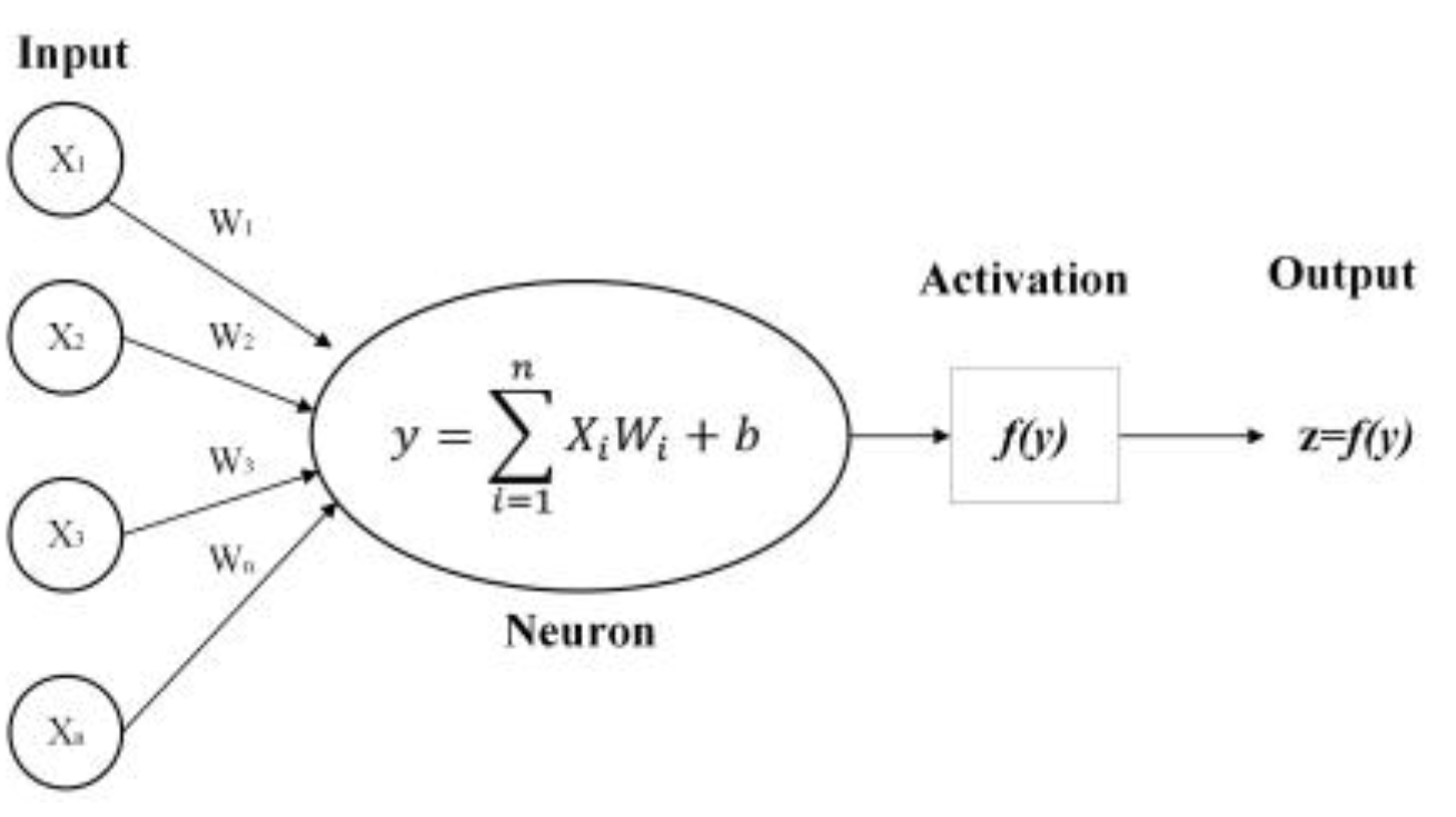
Artificial Neural Networks (ANN) are powerful machine learning models that perform tasks such as data analysis, prediction, and classification based on the working principles of neurons and synapses in the human brain [
19]. ANN, which forms the basis of deep learning techniques, can make high-accuracy predictions on large and complex data sets. The simplest processing unit in an ANN is a single-layer perceptron called a neuron (see
Figure 4)[
20].
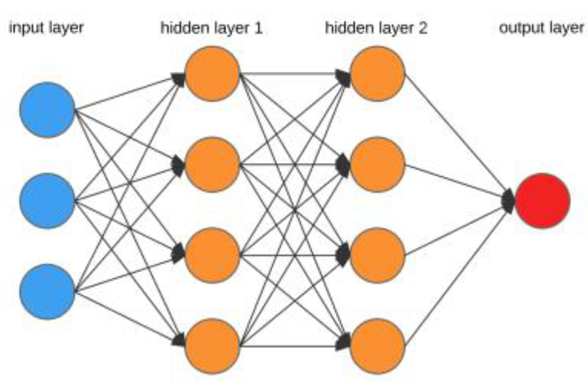
An Artificial Neural Network (ANN) consists of three basic components: input layer, hidden layers, and output layer. The features in the data set are processed in the input layer and transferred to the model [
21]. In the hidden layer, each neuron processes the weighted sum it receives from the inputs connected to it through an activation function. The final prediction value is produced in the output layer. The multilayer perceptron model works by progressing from the input layer to the output layer, as shown in
Figure 5[
20].
The activation of each neuron (
a=f(z)) is calculated using Equation 8.
where
wi weight values,
xi input values,
b bias term,
f(z) activation function, and
a output obtained as a result of activation.
In ANN models, activation functions increase the learning capacity of the network by providing a nonlinear transformation of the input. Common activation functions are ReLU, Sigmoid, and Tanh (Hyperbolic Tangent) functions. In this study, the ReLU function (f(x)= max(0, x)) is preferred because it enables the model to learn faster by zeroing out negative values and minimizes the vanishing gradient problem [
22].
ANN models are trained with backpropagation and gradient descent algorithms. The Forward Propagation method passes input data through neurons to create predictions [
23]. The error between the true values (
Dse) and the predicted values is determined. The Backpropagation method updates the error by distributing it to the weights and bias terms with chained derivative calculations. With the Gradient Descent method, the weights are updated according to the learning rate (
α) using Equation 9.
where
L is the loss function (i.e., Mean Squared Error - MSE),
α is the learning rate, and
w is the weights of the model. This process continues for a certain number of iterations (epochs), and the model is trained until the error rate is minimized.
It can learn complex relationships and successfully model nonlinear structures. It reduces the need for feature engineering because it can perform automatic feature extraction. It can work effectively on large data sets with parallel computation. Computational cost is high, large network structures require high processing power. It is prone to overfitting; regularization techniques are required. Hyperparameter tuning is difficult; extensive experiments are required for the optimum structure.
The performance of the ANN model will be evaluated with MSE, RMSE, and R2 metrics. The ANN model will be used to estimate the equilibrium scour depth (Dse) around the bridge side piers by comparing it with other regression models in this study.
3. Results
In this study, different regression models were applied and evaluated to estimate the equilibrium scour depth (
Dse) around the bridge piers. The dataset used in the machine learning models was divided into 80% model training and 20% testing. Each of the models was trained using training data, and testing was performed using test data. MSE, RMSE, and R
2 metrics were used to evaluate the performance of machine learning models. MSE is the average of the squared differences between the actual values and the predicted values. This error metric measures how successful the model is in making correct predictions. RMSE is the square root of MSE and takes the square root of the average of the differences between the actual values and the predicted values. Therefore, the biggest difference between RMSE and MSE is that it acts like a punisher by giving more weight to large errors with this mathematical operation. On the other hand, it rewards very small errors, so to speak. R² is a measure of the agreement between the actual value and the model's predictions. It is found by dividing the variance of the actual values by the variance of the predicted values. The R
2 value takes a value between 0% and 1%, and a value of 1% means that the model explains the data perfectly and the model fits perfectly. The metrics of the models are shown in
Table 2.
When the metrics of the models are examined in
Table 2, the best performance values were achieved by DTR (99.28%), XGBoost (99.21%), ANN (98.77%) and RFR (95.63%) machine learning models, respectively. With these models, predictions with high accuracy rates were made using test data.
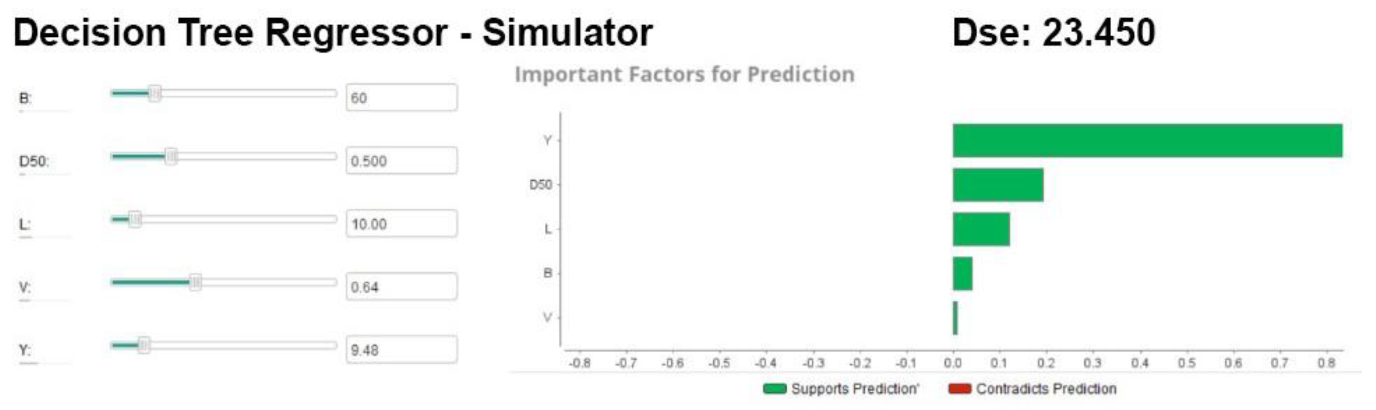
A simulator application code was written for the DTR model that showed the highest performance value, and testing was performed on it, as shown in
Figure 6. For the testing process, the values of 9.48, 10.0, 60, 0.500, and 0.64 were entered for the
Y, L, B, D50, and
V features, respectively, and the equilibrium scour depth (
Dse) value around the bridge piers was estimated as 23.450. It was determined that the estimated value had a high accuracy rate. The predicted values of all models used in the study are also shown in
Table 3.
The predicted values of all models used in the study are also shown in
Table 3.
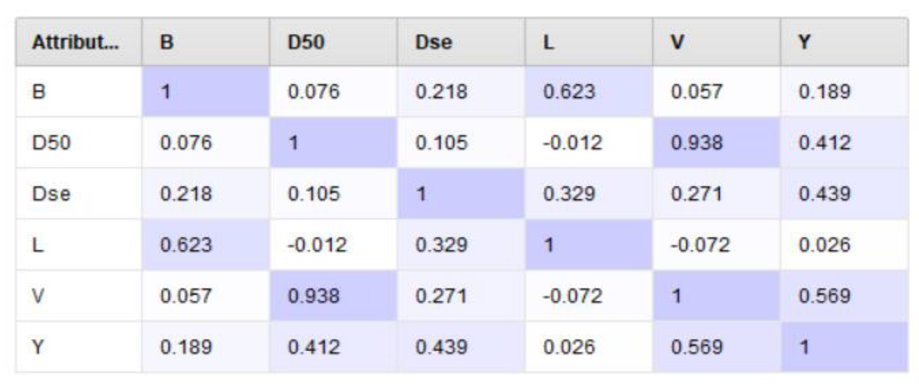
The correlation distribution matrix of the features in the dataset is shown in
Figure 7. The correlation matrix shows the relationships between the features and their effects on each other.
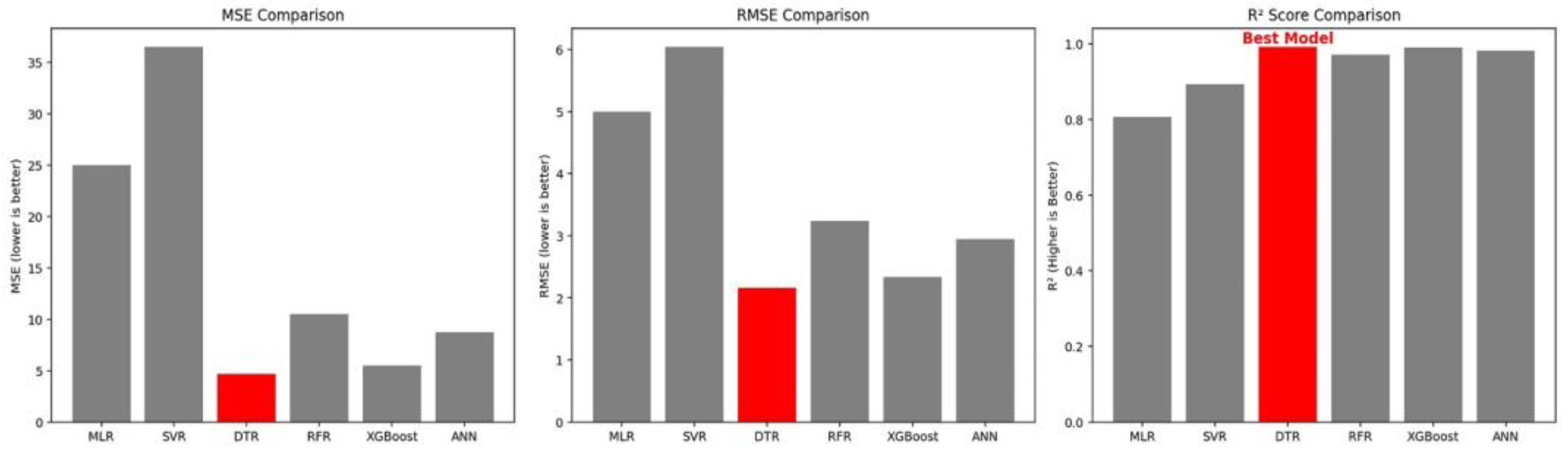
Performance comparisons of the models using MSE, RMSE, and R
2 metrics are shown in
Figure 8. As can be seen from the graphs, the best model that performs the prediction process on the dataset used is the Decision Tree Regression model.
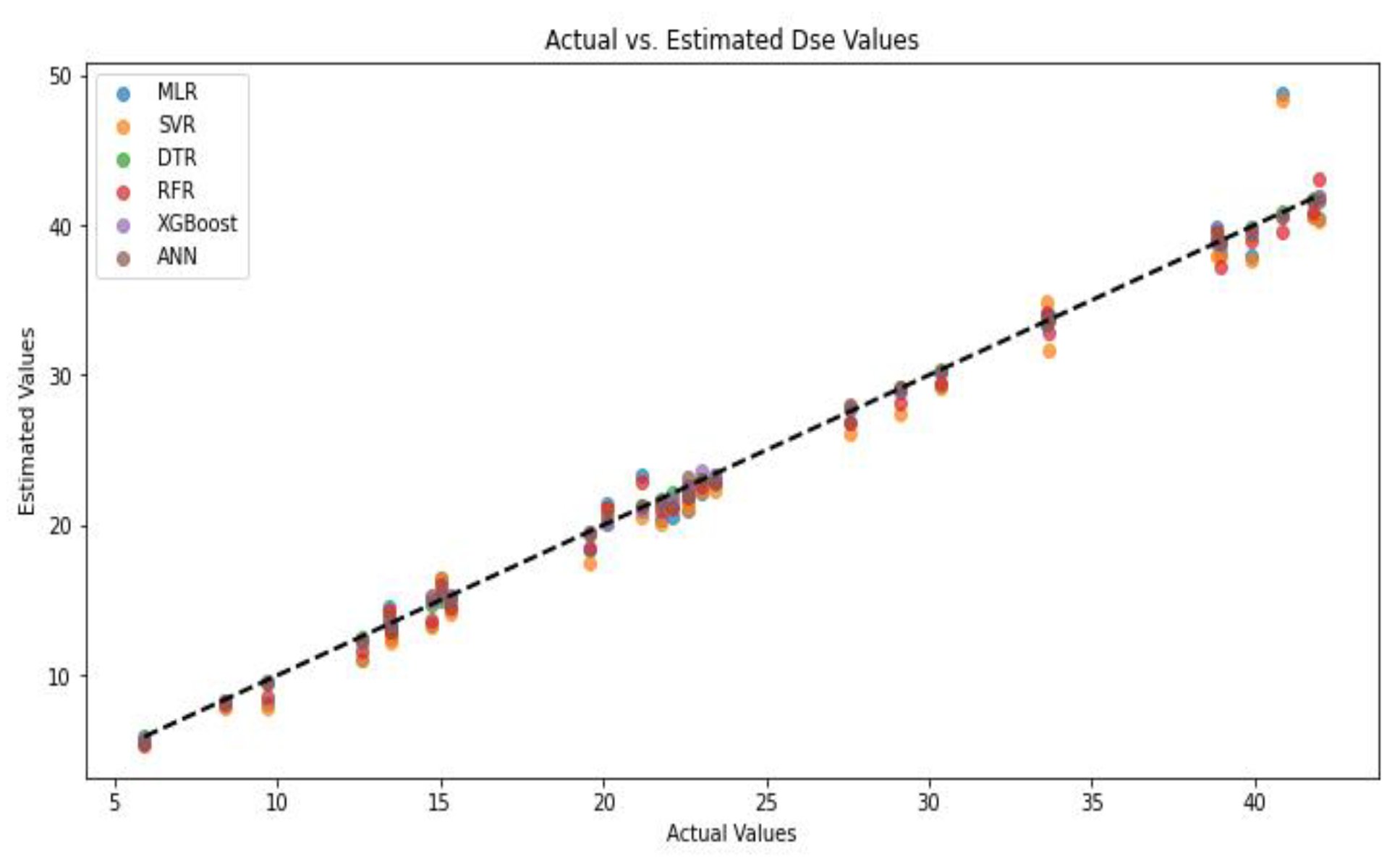
The graph showing the actual
Dse values in the dataset and the
Dse values predicted by the models together is shown in
Figure 9.
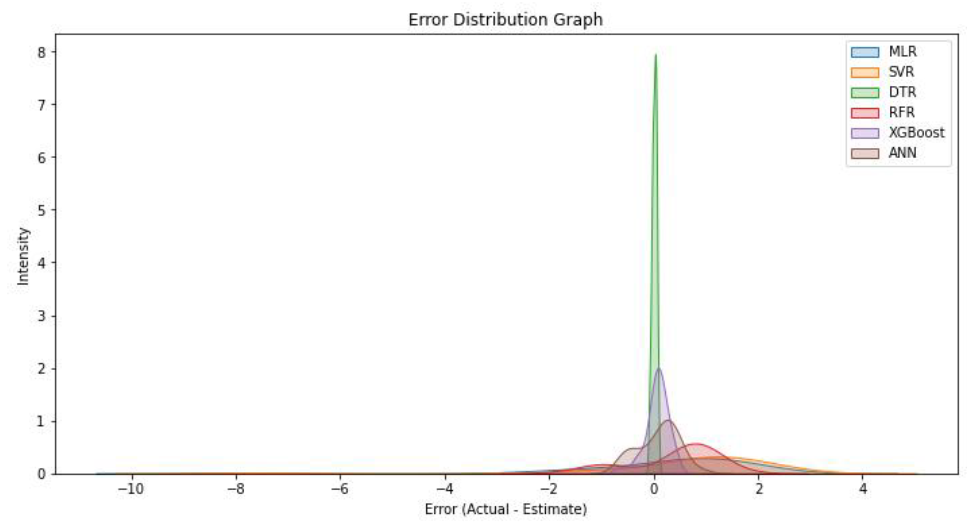
The error distribution graphs of the models are shown in
Figure 10.
4. Discussion
This study investigated the estimation of equilibrium scour depth (Dse) around bridge abutments using various artificial intelligence (AI) models, including Multiple Linear Regression (MLR), Support Vector Regression (SVR), Decision Tree Regressor (DTR), Random Forest Regressor (RFR), XGBoost, and Artificial Neural Networks (ANN). The results indicate that AI-based methods, particularly ensemble learning models and deep learning techniques, offer significant improvements over traditional regression approaches in terms of predictive accuracy and generalization capabilities.
One of the key findings of this study is that the Decision Tree Regressor (DTR) model achieved the highest accuracy (99.28%) in predicting Dse, closely followed by XGBoost (99.21%) and ANN (98.77%). These models demonstrated superior performance due to their ability to capture complex nonlinear relationships between hydraulic parameters and scour depth. Traditional statistical models like MLR, which rely on linear assumptions, were observed to have lower accuracy, emphasizing the necessity of more advanced machine learning techniques for such predictive tasks.
The superiority of ensemble learning techniques, such as Random Forest and XGBoost can be attributed to their robust handling of high-dimensional data and ability to mitigate overfitting by aggregating multiple decision trees. Similarly, the ANN model, leveraging deep learning principles, exhibited strong generalization performance by efficiently learning patterns within the dataset. However, its slightly lower accuracy compared to tree-based methods suggests that feature selection and hyperparameter tuning could further enhance its performance.
Despite their high predictive power, AI models also have certain limitations. Computational complexity and training time were observed to be key challenges, particularly for ANN and XGBoost models. The need for large datasets to achieve reliable generalization is another consideration, as data sparsity may lead to reduced performance in real-world applications. Furthermore, while AI models provide accurate predictions, they do not inherently offer physical insights into the scour process, which remains a crucial aspect of hydraulic engineering.
A comparison with experimental measurements showed a strong correlation between observed and predicted values, reinforcing the validity of AI-based scour depth estimation methods. The application of AI models in bridge design and maintenance planning presents a promising avenue for future research, particularly in integrating real-time monitoring data with predictive analytics to enhance structural safety.
Future studies could explore hybrid AI models that combine physical modeling principles with data-driven approaches to improve interpretability while maintaining high accuracy. Additionally, extending the dataset with more diverse hydraulic conditions and optimizing model architectures through automated machine learning (AutoML) techniques could further refine prediction capabilities.
Overall, this study highlights the potential of AI-driven methodologies in hydraulic engineering and infrastructure safety, providing a reliable and efficient alternative to conventional scour estimation techniques. The integration of such advanced computational models in practical engineering applications can significantly enhance decision-making processes, ultimately contributing to more resilient and sustainable bridge designs.
5. Conclusions
This study demonstrated the effectiveness of artificial intelligence models in predicting equilibrium scour depth (Dse) around bridge abutments. Among the models tested, Decision Tree Regressor (DTR), XGBoost, and Artificial Neural Networks (ANN) achieved the highest accuracy, indicating that machine learning techniques can significantly improve the estimation of scour depth compared to traditional empirical methods.
The findings highlight the potential of AI-driven approaches for enhancing bridge safety by providing reliable scour depth predictions. These models successfully captured the nonlinear relationships between hydraulic and sedimentological parameters, offering an effective alternative to conventional regression-based techniques. The integration of AI into hydraulic engineering can contribute to improved infrastructure design, early risk assessment, and cost-effective maintenance strategies.
While AI models provide high accuracy, certain challenges remain, such as computational complexity, the need for large datasets, and interpretability issues. Future research should focus on optimizing model architectures, incorporating hybrid AI-physical modeling approaches, and utilizing real-time monitoring data to refine predictive capabilities.
In conclusion, this study underscores the transformative impact of artificial intelligence in hydraulic engineering. The use of advanced machine learning models can provide more accurate, efficient, and data-driven solutions for scour depth estimation, ultimately contributing to safer and more resilient bridge structures.
Author Contributions
Conceptualization, Y.U and ŞYK.; Data curation, Y.U and ŞYK.; Formal analysis, Y.U.; Investigation, Y.U and ŞYK; Methodology, Y.U; Supervision, Y.U.; Visualization, Y.U.; Writing—original draft, Y.U.; Writing—review & editing, Y.U and ŞYK. All authors have read and agreed to the published version of the manuscript.
Funding
This research received no external funding.
Data Availability Statement
We encourage all authors of articles published in MDPI journals to share their research data. In this section, please provide details regarding where data supporting reported results can be found, including links to publicly archived datasets analyzed or generated during the study. Where no new data were created, or where data is unavailable due to privacy or ethical restrictions, a statement is still required. Suggested Data Availability Statements are available in the section “MDPI Research Data Policies” at
https://www.mdpi.com/ethics.
Acknowledgments
The authors are indebted to Prof. Dr. Francesco Ballio for supplying the experimental data and the Technical Research and Quality Control Laboratory of General Directorate of State Hydraulic Works for the experimental study.
Conflicts of Interest
The authors declare no conflict of interest.
Abbreviations
The following abbreviations are used in this manuscript:
| MLR |
Multiple Linear Regression |
| SVR |
Support Vector Regression |
| DTR |
Decision Tree Regressor |
| RFR |
Random Forest Regressor |
| ANN |
Artificial Neural Networks |
| Dse |
Equilibrium Scour Depth |
| Y |
Flow Depth |
| L |
Abutment Length |
| B |
Channel Width |
| V |
Flow Velocity |
| D50 |
Median Grain size |
References
- Melville, B.W.; Coleman, S.E. Bridge Scour; Water Resources Publication: Littleton, Colorado, 2000. [Google Scholar]
- Federal Highway Adminisration Evaluating Scour At Bridges. 2001.
- Lee, T.L.; Jeng, D.S.; Zhang, G.H.; Hong, J.H. Neural Network Modeling for Estimation of Scour Depth Around Bridge Piers. J Hydrodyn 2007, 19, 378–386. [Google Scholar] [CrossRef]
- Azamathulla, H.Md.; Deo, M.C.; Deolalikar, P.B. Alternative Neural Networks to Estimate the Scour below Spillways. Advances in Engineering Software 2008, 39, 689–698. [Google Scholar] [CrossRef]
- Zounemat-Kermani, M.; Batelaan, O.; Fadaee, M.; Hinkelmann, R. Ensemble Machine Learning Paradigms in Hydrology: A Review. Journal of Hydrology 2021, 598, 126266. [Google Scholar] [CrossRef]
- Hamidifar, H.; Zanganeh-Inaloo, F.; Carnacina, I. Hybrid Scour Depth Prediction Equations for Reliable Design of Bridge Piers. Water 2021, 13, 2019. [Google Scholar] [CrossRef]
- Khan, Z.U.; Khan, D.; Murtaza, N.; Pasha, G.A.; Alotaibi, S.; Rezzoug, A.; Benzougagh, B.; Khedher, K.M. Advanced Prediction Models for Scouring Around Bridge Abutments: A Comparative Study of Empirical and AI Techniques. Water 2024, 16, 3082. [Google Scholar] [CrossRef]
- Kumcu, S.Y.; Kokpinar, M.A.; Gogus, M. Scour Protection around Vertical-Wall Bridge Abutments with Collars. KSCE J Civ Eng 2014, 18, 1884–1895. [Google Scholar] [CrossRef]
- Mihaly Cozmuta, L. The Application of Multiple Linear Regression Methods to FTIR Spectra of Fingernails for Predicting Gender and Age of Human Subjects. Heliyon 2025, 11, e42815. [Google Scholar] [CrossRef] [PubMed]
- Luo, M.; Liu, M.; Zhang, S.; Gao, J.; Zhang, X.; Li, R.; Lin, X.; Wang, S. Mining Soil Heavy Metal Inversion Based on Levy Flight Cauchy Gaussian Perturbation Sparrow Search Algorithm Support Vector Regression (LSSA-SVR). Ecotoxicology and Environmental Safety 2024, 287, 117295. [Google Scholar] [CrossRef] [PubMed]
- Xiong, L.; An, J.; Hou, Y.; Hu, C.; Wang, H.; Chen, Y.; Tang, X. Improved Support Vector Regression Recursive Feature Elimination Based on Intragroup Representative Feature Sampling (IRFS-SVR-RFE) for Processing Correlated Gas Sensor Data. Sensors and Actuators B: Chemical 2024, 419, 136395. [Google Scholar] [CrossRef]
- Pedrós Barnils, N.; Schüz, B. Identifying Intersectional Groups at Risk for Missing Breast Cancer Screening: Comparing Regression- and Decision Tree-Based Approaches. SSM - Population Health 2025, 29, 101736. [Google Scholar] [CrossRef] [PubMed]
- Effects of Tuning Decision Trees in Random Forest Regression on Predicting Porosity of a Hydrocarbon Reservoir. A Case Study: Volve Oil Field, North Sea. Energy Advances 2024, 3, 2335–2347. [Google Scholar] [CrossRef]
- Sánchez, J.C.M.; Mesa, H.G.A.; Espinosa, A.T.; Castilla, S.R.; Lamont, F.G. Improving Wheat Yield Prediction through Variable Selection Using Support Vector Regression, Random Forest, and Extreme Gradient Boosting. Smart Agricultural Technology 2025, 10, 100791. [Google Scholar] [CrossRef]
- Ramos Collin, B.R.; de Lima Alves Xavier, D.; Amaral, T.M.; Castro Silva, A.C.G.; dos Santos Costa, D.; Amaral, F.M.; Oliva, J.T. Random Forest Regressor Applied in Prediction of Percentages of Calibers in Mango Production. Information Processing in Agriculture 2024. [Google Scholar] [CrossRef]
- EL Bilali, A.; Hadri, A.; Taleb, A.; Tanarhte, M.; EL Khalki, E.M.; Kharrou, M.H. A Novel Hybrid Modeling Approach Based on Empirical Methods, PSO, XGBoost, and Multiple GCMs for Forecasting Long-Term Reference Evapotranspiration in a Data Scarce-Area. Computers and Electronics in Agriculture 2025, 232, 110106. [Google Scholar] [CrossRef]
- Cheng, T.; Yao, C.; Duan, J.; He, C.; Xu, H.; Yang, W.; Yan, Q. Prediction of Active Length of Pipes and Tunnels under Normal Faulting with XGBoost Integrating a Complexity-Performance Balanced Optimization Approach. Computers and Geotechnics 2025, 179, 107048. [Google Scholar] [CrossRef]
- Alsulamy, S. Predicting Construction Delay Risks in Saudi Arabian Projects: A Comparative Analysis of CatBoost, XGBoost, and LGBM. Expert Systems with Applications 2025, 268, 126268. [Google Scholar] [CrossRef]
- García, L.C.H.; Valencia, J.V.; Colorado L, H.A. Modeling an Artificial Neural Network to Estimate Cement Consumption in Clayey Waste-Cement Mixtures Based on Curing Temperature, Mechanical Strength, and Resilient Modulus. Construction and Building Materials 2025, 467, 140376. [Google Scholar] [CrossRef]
- Uzun, Y.; Saltan, F.Z. Use of Machine Learning Methods in Predicting the Main Components of Essential Oils: Laurus Nobilis L. Journal of Essential Oil Bearing Plants 2024, 27, 1302–1318. [Google Scholar] [CrossRef]
- Okoro, O.V.; Hippolyte, D.C.; Nie, L.; Karimi, K.; Denayer, J.F.M.; Shavandi, A. Machine Learning-Based Predictive Modeling and Optimization: Artificial Neural Network-Genetic Algorithm vs. Response Surface Methodology for Black Soldier Fly (Hermetia Illucens) Farm Waste Fermentation. Biochemical Engineering Journal, 2025; 109685. [Google Scholar] [CrossRef]
- Abushandi, E. Water Quality Assessment and Forecasting Along the Liffey and Andarax Rivers by Artificial Neural Network Techniques Toward Sustainable Water Resources Management. Water 2025, 17, 453. [Google Scholar] [CrossRef]
- Tran, T.V.; Peche, A.; Kringel, R.; Brömme, K.; Altfelder, S. Machine Learning-Based Reconstruction and Prediction of Groundwater Time Series in the Allertal, Germany. Water 2025, 17, 433. [Google Scholar] [CrossRef]
|
Disclaimer/Publisher’s Note: The statements, opinions and data contained in all publications are solely those of the individual author(s) and contributor(s) and not of MDPI and/or the editor(s). MDPI and/or the editor(s) disclaim responsibility for any injury to people or property resulting from any ideas, methods, instructions or products referred to in the content. |
© 2025 by the authors. Licensee MDPI, Basel, Switzerland. This article is an open access article distributed under the terms and conditions of the Creative Commons Attribution (CC BY) license (http://creativecommons.org/licenses/by/4.0/).