
Submitted:
11 September 2024
Posted:
11 September 2024
You are already at the latest version
Abstract
The fundamental period is one of the most important parameters for the design of new structures , as well as the estimation of the capacity of existing ones. However, its calculation requires the solution of an eigenvalue problem. Especially for new buildings, this can involve material and geometric parameters that are not known beforehand. Thus, to estimate it, various design codes and researchers have adopted a several approximate analytical equations based on a number of key structural parameters. To this end, the present study introduces a novel methodology for the derivation of analytical equations for the fundamental period of Reinforced Concrete (RC) structures. The methodology is based on Machine Learning (ML) explainability techniques and specifically the so-called SHapley Additive exPlanations (SHAP) values. The novel methodology allows these equations to be constructed sequentially and in an informed manner, controlling the balance between accuracy and complexity. An extended dataset comprised of 4026 data points is employed. The results showed excellent accuracy, with a coefficient of determination R2≈0.95. This demonstrates the potential applicability of the proposed methodology in a wide array of similar engineering challenges.
Keywords:
fundamental period
; masonry infilled framed structures
; machine learning
; explainability
; SHAP
; analytical equations
1. Introduction
The Fundamental Period (FUP) of buildings is a very important parameter in the context of new structures’ seismic design. Moreover, it is a crucial feature that can be used for the determination of existing buildings’ seismic capacity [1,2]. The design spectrum of available seismic codes, combined with the estimated FUP, can lead to the determination of the forces introduced by a seismic excitation in a building, i.e.,, the calculation of the seismic base shear. Furthermore, FUP is a crucial feature that can be employed for the near real time estimation of the seismic forces introduced on the buildings, by a strong seismic excitation (under the corresponding acceleration spectrum). In this way, the level of seismic damage can be macroscopically estimated and documented [3,4].
However, as it is well known, the calculation of the fundamental period, requires the solution of an eigenvalue problem. The formulation and solution of this problem, under the finite elements’ framework, requires the knowledge of the values of numerous parameters to be used for the estimations of the stiffness and of the mass matrices of buildings [5,6]. Furthermore, in the case of designing new buildings, the values of the above parameters cannot be known before the final design. Therefore, it is particularly useful to develop approximation methods for the estimation of FUP. This can be achieved either by considering only some of the problem’s parameters that can be easily calculated at the design stage of new buildings, or by directly estimating them by working already existing buildings (e.g., buildings for which a rapid assessment of their seismic capacity has been performed before or after a strong seismic excitation).
In particular, for the case of new reinforced concrete (RC) buildings, the respective design codes [7,8,9,10,11,12,13,14,15,16,17,18] have globally incorporated in the last decades approximate equations for the estimation of FUP, recognizing its usefulness in the design process. However, in addition to the codes, the formulation of approximate equations for the calculation of the fundamental period has been the subject of a significant number of research papers [19,20,21,22,23,24,25,26,27,28,29,30,31,32,33]. These research studies have utilized instrumental measurements of buildings during strong seismic excitations, as well as measurements of ambient vibrations. In addition, numerical finite element models have been used in order to increase the number of buildings based on which the FUP equations have been developed. The obtained results were used to document the existing approximate equations of the codes and to improve them.
One of the parameters that can significantly affect the value of the fundamental period, are the masonry infills. It has been shown, through a series of numerical and experimental researches, that masonry infills can significantly increase the horizontal stiffness of Reinforced Concrete (RC) buildings, resulting in a significant change in the seismic forces they receive. Thus, the specific research to assess the influence of masonry infills on the FUP approximation equations, has been the subject of a significant number of research papers [34,35,36,37,38,39,40,41,42,43,44].
Statistical processing of instrumental measurements or results obtained from computational analyses is a basic research approach aiming at the formulation of approximate equations for the estimation of FUP in RC buildings. This can be done with or without masonry infills. Therefore, the problem is reduced to the processing of available databases, containing values of the fundamental periods of buildings with different structural characteristics. In this regard, the recent rapid increase in the use of machine learning (ML) algorithms for solving civil engineering problems [45,46,47,48,49] has has given a new perspective to the investigation of equations for estimating the fundamental periods of RC buildings with masonry infills (RCB_MI). The inherent ability of ML algorithms in handling large volumes of data and their potential in modeling multiparametric cases [50,51,52,53,54]) has led to their engagement as the main modeling tools for the estimation of FUP in infilled RC buildings.
1.1. Literature Review
Kose [55] developed relationships for calculating the fundamental period of masonry infilled buildings, using a multiple Linear Regression model. To investigate the structural parameters that most influence the value of the fundamental period he performed sensitivity analyses using Feed-Forward Artificial Neural Networks (ANN) with one hidden layer. Thus, he derived models that correlate FUP with the height, the percentage of RC walls and the percentage of masonry infills of the buildings.
Asteris developed a dataset [56] that was suitable for training ML algorithms to develop simplified equations for the estimation of the fundamental period of RCB_MI. This dataset has been used by other researchers and it is briefly described in Section 2.1 of the present paper. Asteris et al. [57] used the above dataset [56] to train feed-forward ANNs with one or two hidden layers. The developed model offered values for the fundamental period of infilled RC buildings. These values have been compared with the ones derived from the equations suggested by the codes. These comparisons have shown that the correlation between the FUP and the structural parameters (e.g., the buildings’ height, the number and the length of their openings, the strength and the percentage of masonry infills) leads to more realistic results than the correlation of the fundamental period with the height of the buildings, that was proposed by most available codes. In a later study, Asteris and Nikoo [58] used the aforementioned dataset [56] to train feed-forward ANNs which were optimized via an artificial bee colony optimization algorithm. Using this methodology, they obtained high correlation coefficients between the considered structural parameters (building height, number and length of openings, as well as strength and percentage of masonry infills) and the fundamental period.
Charalampakis et al., [59] used the same dataset [56] to train feed-forward ANNs with two or three hidden layers (which can be considered too complicated to offer a model that can generalize). They also applied the M5Rules algorithm, which belongs to the group of decision tree learners. They finally arrived at a set of simplified equations for computing the fundamental period as a function of: the number of storeys, the stiffness of the infill walls and the frames’ span length. They derived separate equations for different masonry infill ratios (opening ratio from 0% for bare frames to 100% for fully infilled RC frames) and a single equation for all masonry infill rates (opening ratios).
Somala et al., [60] applied a series of ML algorithms (linear regression, ridge regression, k-nearest neighbors, support vector regression, random forest, decision tree, extreme gradient boosting and adaptive boosting) using the above training dataset created by Asteris [56]. From their study they reached the main conclusion that the XGBoost algorithm is the most effective algorithm for predicting the value of the FUP. Moreover, they also concluded that the number of storeys is the most important structural parameter. This conclusion is consistent with the choice of most codes to relate the FUP to the height of RC buildings.
Mirrashid and Naderpour [61] applied a feed forward neural network model with one hidden layer and a Neuro Fuzzy (ANFIS) one [62] based on the Asteris dataset [56]. They tried to derive equations for computing the FUP values. For their study they used the dataset developed by Asteris [56]. One of their most remarkable conclusions was that the most effective parameter for the calculation of the fundamental period is the masonry infills ratios of the frames (opening ratios).
Yahiaoui et al., [63] used three Boosting ML models (LightGBM, Gradient Boosting Decision Trees and CatBoost) which they trained with the Asteris training dataset [56]. Moreover, by applying the “Multivariate Adaptive Regression Spline” technique they arrived at an approximate equation for computing the FUP values. From the comparisons they made with similar relations available in the literature, they concluded that the combined use of the LightGBM model and the Multivariate Adaptive Regression Spline technique leads to the most efficient relation both in terms of the level of Accuracy and avoidance of Overfitting effects.
Thisovithan et al., [64] used four ML algorithms (Artificial Neural Network, k-Nearest Neighbors, Support Vector regression, and Random Forest). The results of these models were interpreted using three different Post-Hoc explanations. We should clarify that Post-hoc explainability methods analyze and interpret the decision-making process of a trained model after it has made predictions, providing insights into how the model arrived at its outputs. In addition, they developed an (Explainability) XAI-based user interface [65] through which it is possible to input the appropriate structural data/parameters and to obtain the automatic extraction of the estimated fundamental period. By using this application, it is possible to achieve in real time the selection of structural parameters in order to optimize the design of the infilled RC frames and to interpret how each structural parameter influences the final result.
1.2. Novelty and Contribution of the Research
This research has strong elements of novelty, as it introduces an explainable modeling approach using the SHapley Additive exPlanations (SHAP values). The SHAP Machine Learning explainability methodologies, are used to provide interpretable, analytical equations that approximate the behavior of the underlying ML model. They quantify each feature’s importance based on the predictive power it contributes, accounting for complex feature interactions. They employ Game Theory to assign credit to each feature, or feature value, resulting in the prediction capacity of the developed model. The way SHAP works is to decompose the output of a model by the sums of the impact of each feature. As it will be shown, SHAP values are feature attribution methods, i.e.,, they analyze the predictions of the ML model into components pertaining to each individual feature. However, in the currently established literature, this methodology is employed as an explainability tool, i.e.,, to quantify the effect of each input parameter on the model’s prediction [60,64]. In our proposed formulation, SHAP values are not only used in this regard, but in addition, departing from the currently established literature, they have been employed as a basis for the creation of interpretable, simplified, analytical equations that approximate the behavior of the underlying ML model.
Thus, the benefit of the proposed formulation is threefold. Firstly, the analytical equations are derived independently and sequentially. Secondly, again by utilizing the SHAP values, features are inserted into the simplified model in an informed manner, starting from the most important ones. Lastly, this allows a controlled tradeoff between accuracy and model complexity, as dictated by the specific application at hand.
2. Materials and Methods
2.1. Dataset Description
The dataset employed in the present study is the so-called “FP4026 Research Database” introduced by Asteris in 2016 [56]. The dataset consists of 4026 data points, corresponding to infilled Reinforced Concrete plane frames. For each frame, five structural parameters were recorded, namely: 1) the number of storeys 2) the number of spans 3) the length of the spans 4) the masonry walls’ stiffness and 5) the opening percentage, i.e.,, the percentage of the panel area covered by the infill walls. The corresponding fundamental period was estimated using the Seismostruct Finite Element Package [66]. The modeling of the infill walls followed the equivalent strut nonlinear cyclic formulation introduced by Crisafulli [67].
The material properties of the frames as well as their dimensions affect the overall stiffness and thus, the fundamental period. In this dataset, the concrete corresponded to C25/30 (25MPa compressive strength and 31GPa modulus of elasticity), while the steel in the reinforcement bars had a strength of 500MPa (corresponding to B500c). The dimensions of the structural members were designed based on EN1998-1 [7]. The beams and slabs had constant dimensions (250/600 and 150 mm, respectively) for all frames. The dimensions of the columns varied with the number of storeys, although this variation is not one of the parameters considered in the present study.
The distribution of the five measured structural parameters as well as the estimated fundamental period is shown in the following Figure 1. The number of storeys ranged uniformly between 1 and 22, while the number of spans was either 2, 4, or 6, with the majority of the frames (65%) had 6 spans. The corresponding length of the spans was uniformly distributed between 3, 4.5, and 6 meters, with a smaller number of structures having 7.5m span length. The masonry wall stiffness ranged from 2.25 to 25 kN/m, while the corresponding opening percentage ranged from 0 to 100%, with approximately 46% of the cases corresponding to bare frames.
2.2. Data Preprocessing
Following the above observations, we preprocessed the available dataset as follows: Firstly, we scaled the opening percentage to the [0,1] range so that its values are not much larger than the rest of the features. Subsequently, we transformed the given fundamental period using the natural logarithm. This ensures that any regression model will output strictly positive values, by using the inverse exponential transformation. Finally, even though, as was mentioned, 46% of the cases were bare frames, the corresponding data points had values for the masonry wall stiffness that covered the entire range of that feature. However, such data points don’t make physical sense. Thus, from a mathematical point of view, any regression model trained using these data points is trained on non-physical data points. To this end, in the present study, we removed the corresponding stiffness values, treating them as NaN’s (“not a number”, missing value). As we will examine in the sequel, this modeling decision affects the choice of regression models, as well as the computation of SHAP values.
2.3. Machine Learning Modeling
One can try and compare all available algorithms which have the potential of offering high accuracy. However, the most important aim of our research team is not to find the “one and only optimal model” for a specific dataset and another “optimal” one for another dataset. A more realistic target is to develop a low complexity model, that can effectively generalize with high accuracy, capable of avoiding overfitting, and easily adjustable. This can be ensured by employing Explainability techniques and more specifically in this study by estimating respective SHAP values. This can lead to the potential development of simplified analytical equations. Thus, our trained ML model must exhibit a high enough accuracy level, so that the obtained SHAP values are reliable, without having overfitted on the available dataset. To this end, there are many available regression models in the literature.
In this study, we have employed a Gradient Boosting Machine [68], which offers several advantages. First, it is a powerful algorithm that combines a group of “weak models” to produce an Ensemble model, in an iterative procedure known as Boosting [68], wherein the errors from each iteration are used as input in the next. Specifically, the algorithm employs the following learning function seen in equation (1).
In the above equation, are the “weak models”, which are usually Decision Trees, although other models have been employed as well [69]. In addition, are the learned parameters of each individual model, are the learned weights used for the ensembling, and N is the user defined maximum number of base models. In the present study, we used a maximum number of trees, each with a maximum depth of 5.
The models’ hyperparameters were determined typically by using a trial an error approach. As it has already been mentioned, the aim of this study is not to identify “the best” model, but rather a model with high enough accuracy and, at the same time, low complexity, to avoid overfitting on the particular dataset.
One additional advantage of the employed algorithm is that it natively supports Not a Number (NaN) values, which, as we mentioned, we introduced into the dataset as part of the preprocessing. These NaN values are somewhat restrictive with regards to the choice of the regression model, as not all algorithms support them, but they have two distinct advantages. On the one hand, they are conceptually correct. On the other hand, SHAP values, which are central to our formulation, model NaN values exactly, as we will discuss in the sequel.
2.4. Shapley Additive Explanations (SHAP)
SHapley Additive exPlanations (SHAP) is a machine learning explainability technique recently developed by Scott Lundberg [70]. Intuitively, SHAP values decompose the ML model’s predictions into a summation of terms corresponding to each individual feature. They do this by extending the so-called Shapley values [71] from cooperative game theory, proposed by Lloyd Shapley in 1951. Formally, given a trained ML model f, a local approximation g is defined as follows (equation (2))
where m is the number of features, is the mean model prediction, are the SHAP values, and is the so-called “simplified input” [70] , i.e.,, a binary vector whose value shows whether or not the corresponding feature was missing. Thus, for each data point, the model’s predictions is decomposed into terms pertaining to each individual term, and a constant term, i.e.,, the average prediction. In addition, SHAP values satisfy an important property called missingness [70], which states that features whose value is missing have no contribution to the model, i.e.,,
Following the notation of Lundberg and Su-In [70], let be the complete feature set that was employed and let be a subset. Then, the coefficients are given by the following equation (4)
The intuitive interpretation of the above equation is that the SHAP values are a weighted average over all possible feature combinations of the gain in the model’s prediction when feature i is included. From the above it becomes apparent that if the underlying ML model has a high enough accuracy, the sum of the corresponding SHAP values will also be close to the true target values.
3. Results
As it has been previously stated, the aim of this study is to employ explainability techniques and SHAP values in particular to derive simple, analytical, and additive formulas for the estimation of the fundamental period. To ensure that these SHAP values are reliable, they must be derived from a ML model that has not overfitted to the available dataset. Similarly, the trained ML model must have a sufficiently high accuracy, so that its predictions closely resemble the truth.
Thus, in the first part, Section 3.1, we present the results of our fitted ML regression model, that was presented in Section 2.3. We use well-known regression metrics to measure its performance and assess its reliability. Subsequently, in Section 3.2, we present the main results of this study and we demonstrate how SHAP values can be employed to provide simplified, analytical equations that can be used in lieu of the complex ML model. We also see how these equations can be obtained in an incremental manner, which is important, as in this way complexity can be added or removed according to the desired level of accuracy.
3.1. Machine Learning Regression
As it was mentioned in Section 2.3, we employed a Gradient Boosting Machine learning for the regression task, using a maximum number of trees, each with a maximum depth of 5. We arrived at this configuration using a trial and error approach, as these hyperparameters achieved an excellent accuracy, without an enormous amount of complexity. We trained the model using a so-called 75-25 split, i.e.,, 75% of the dataset were randomly selected for training, while the remaining 25% was the dataset used to gauge the model’s performance on truly unseen data. We used the well-known regression metrics of Mean Absolute Error (MAE), Root Mean Squared Error (RMSE), and Coefficient of Determination . Their corresponding formulae are shown in Table 1. Table 2 summarizes their computed values on both the training and testing datasets, both in the log-transformed space, as well as in the original space, by using the inverse exponential transformation.
We can readily observe that the trained ML model achieved excellent performance in both the Log-Transformed and the original space, with a value of equal to and , respectively. In addition, the performance is similar in both cases between the training and test dataset, indicating that the model did not overfit. Finally, the values of MAE and RMSE were low and relatively close to each other. This indicates that the trained model did not have many large values in its errors. Such errors are accentuated when squared in the calculation of RMSE and, thus, this effect would manifest via a large discrepancy between RMSE and MAE which is not present in our case.

Table 1.
Formulae of the employed regression metrics. The true and predicted values are denoted by and , respectively, while N denotes the total number of data points.
Table 1.
Formulae of the employed regression metrics. The true and predicted values are denoted by and , respectively, while N denotes the total number of data points.
| Metric | Formula |
|---|---|
| MAE | |
| RMSE | |
Table 2.
Regression metrics on the training and test dataset of the fully trained ML model.
| Log-transformed | Original space | |||
|---|---|---|---|---|
| Training | Test | Training | Test | |
| MAE | 0.0487 | 0.0517 | 0.0524 | 0.0545 |
| RMSE | 0.0645 | 0.0723 | 0.0856 | 0.0870 |
| 0.9943 | 0.9932 | 0.9879 | 0.9879 | |
3.2. Regression Using SHAP
In this Section, we present the main results of our proposed methodology, which focus on employing SHAP values to obtain analytical equations that approximate the predictions of the trained ML model. Furthermore, these equations can be constructed in an incremental manner, wherein accuracy can be increased at the cost of adding more terms and increasing the complexity of the equations.
To this end, we first obtained the SHAP values for each feature and for each data point in the training set. We opted to compute these values on the training and test set separately because we want to utilize them to “train” our simplified equations and, subsequently, test them on the unseen test dataset. Subsequently, we aggregated them using the Mean Absolute value and normalized the results to obtain the percentages, i.e.,, we computed (see equation (5))
In the above equation (5), are the SHAP values of the feature for the data point, N is the total number of data points and M is the total number of features. The results are shown in Figure 2. As it can be readily observed, the most important features by far, were the number of storeys and the opening percentage of the panels, with an overall importance of approximately 50% and 30%, respectively. The stiffness of the masonry walls and the length of the spans had an overall effect of approximately 7-8%, respectively, while the influence of the number of spans was negligible.
The core of the proposed formulation lies in providing analytical approximations to the obtained SHAP values. As it was discussed in Section 2.4, the SHAP values are additive and they sum to the predictions of the ML model. Thus, the advantage of our proposed formulation becomes apparent: we can approximate the SHAP values of each individual feature and add as many terms as required to obtain the desired level of accuracy, guided by the feature importance hierarchy shown in Figure 2. The form of each individual analytical approximation is determined by the corresponding plot of the SHAP values. To demonstrate this, Figure 3 present the scatter plots of the top two features, the number of storeys and the opening percentage, compared with the corresponding plots of the log-transformed fundamental period. For the opening percentage, we present the SHAP values corresponding to 0, 25, 50, and 75% opening percentage, as the bare frame case will be treated separately, as previously discussed.
First, we can readily observe that, while the log-transformed period has a significant variance for a fixed value of number of storeys, the corresponding SHAP values exhibit a much smaller variance. Thus, an analytical curve fitted to the SHAP values, instead of the raw data, will be much more accurate representation of the contribution of this feature to the output. The corresponding SHAP values for the opening percentage exhibits a somewhat larger variance. This is attributed to feature interaction, i.e.,, the contribution of one feature can vary, depending on the value of a different feature [72]. Such interaction effects can be more accurately captured using SHAP interaction values [73]. However, this adds significant complexity to the derived equations. As we will see, in our case the derived equations achieved excellent accuracy. Thus, given that our aim is to derive simple analytical equations, this additional complexity was not justified.
Given the shape of each individual curve, we experimented with a variety of analytical curves for each one, including quadratic polynomials, square roots, logarithms, and exponentials. The results are shown in Table 3. Note that the contribution of the “number of spans” feature was negligible and was ignored. Similarly, the best fitted curve for each feature is presented in Figure 4.
The equations in Table 3 are valid for non-bare frames, i.e.,, cases where the opening percentage was <100%. For bare frames, the contribution of the wall stiffness is set to 0, due to the missingness property (equation (3)). Similarly, when “opening percentage” is equal to 1, as in the bare-frame case, the SHAP values of this feature range from 0.27 to 0.325. Thus, the contribution of this feature for bare frames can be obtained using a single value. As it is well known, the median minimizes MAE while the mean minimizes RMSE. In our case, both the mean and median were very close and approximately equal to 0.33. From the above equations, we selected those with the overall best performance. Finally, note that the above equations only approximate the SHAP values in equation (4). In order for the local approximation (equation (2)) to be accurate, we need to include the constant , i.e.,, the average model prediction. In our case, this was approximately equal to -0.21.
Combining the above, we obtain two analytical equations for the prediction of the fundamental period. Specifically, for bare frames, we obtain
while for non-bare frames we obtain
where in the above equations N is the number of storeys, L is the length of the spans, is the opening percentage (normalized in the [0,1] range) and is the stiffness of the masonry walls.
As it was previously discussed, the benefit of the above formulation is that the number of terms as well as their complexity can be individually adjusted to achieve the desired balance between accuracy and simplicity of the derived formulas.
Using the above, we computed the regression metrics shown in Table 1. We computed them both in the log-transformed space, where the regression was fitted, and in the original space to examine how the inverse exponential transform affects the results. As can be readily observed (Table 4), the regression results using these simplified analytical equations are excellent, achieving low MSE and MAE values and a of approximately 0.97 and 0.95 in the log-transformed and original spaces, respectively. Thus, the proposed relationships can be confidently employed in lieu of the fully trained ML model without a significant loss in accuracy. Finally, due to the excellent regression results, the complexity of adding terms pertaining to SHAP interaction values is not deemed justifiable. However, these terms can be examined in cases where the interactions are significant and high accuracy cannot be achieved using SHAP values alone.
Table 4.
Regression metrics of the simplified analytical equations.
| Log-transformed | Original space | |||||
|---|---|---|---|---|---|---|
| Training | Test | Full dataset | Training | Test | Full dataset | |
| MAE | 0.1185 | 0.1217 | 0.1193 | 0.1174 | 0.1193 | 0.1179 |
| RMSE | 0.1485 | 0.1515 | 0.1493 | 0.1725 | 0.1707 | 0.1721 |
| 0.9706 | 0.9681 | 0.9700 | 0.9522 | 0.9510 | 0.9520 | |
4. Summary and Conclusions
In the framework of the present study, we have utilized ML explainability methodologies, in particular the so-called SHapley Additive exPlanations (SHAP values), are used to provide interpretable, analytical equations that approximate the behavior of the underlying Machine Learning model. We have implemented our proposed methodology on the problem of estimating the fundamental period of buildings, which is a very important parameter in the context of the seismic design of new buildings as well as in the context of the methods used for the evaluation of the seismic capacity of existing buildings.
On the one hand, similar problems of great importance in the engineering community are addressed by various design codes by providing simplified analytical equations that approximate the target variable. On the other hand, ML models have demonstrated their capabilities tackle such problems and to produce state-of-the-art results, with excellent accuracy. This was also demonstrated in the present paper, wherein the fully trained ML model achieved a coefficient of determination . However, ML models often lack interpretability, which hinders their potential to be fully adopted by the engineering community.
Thus, the proposed novel methodology bridges this gap. On the one hand, we employ fully trained ML models, to achieve state-of-the-art results. On the other hand, we utilized the SHAP values explainability techniques as a basis for providing interpretable, analytical equations, which offered distinct advantages compared to the previously established literature.
First, due to the additivity of the SHAP values, the proposed methodology allows for the incremental addition of terms in our simplified analytical equations. Thus, this allows for a controlled tradeoff between model complexity and the desired level of accuracy, according to the application at hand. Second, as Figure 2 demonstrates, SHAP values also allow for a quantification of the percentage of the influence of each individual parameter. Thus, the controlled tradeoff between accuracy and model complexity is not carried out blindly, but rather in an informed manner, guided by the feature importance ranking provided by the SHAP values. Third, due to the fact that SHAP values approximate the behavior of the underlying ML model, the methodology can provide simplified equations with comparable accuracy to the fully trained ML model, as demonstrated in Table 2 and Table 4. Finally, due to the attractive missingness property of SHAP values, missing values, which can potentially be found in many real datasets pertaining to engineering applications, are handled seamlessly and effectively, invalidating the need of imputing them with potentially misleading values.
Thus, even though the proposed methodology was implemented in the frame-work of estimating the fundamental period of buildings, it can be confidently applied to various similar engineering challenges, bridging the gap between the demonstrated power of ML models to produce state-of-the-art results and the need for simplified, analytical equations that instill confidence in the engineering community for their implementation.
Author Contributions
Conceptualization, I.K., K.K., and L.I.; methodology, I.K., K.K., and L.I.; software, I.K., K.K., and L.I.; validation, I.K., K.K., and L.I.; formal analysis, I.K. and K.K.; investigation, I.K., K.K., and L.I.; resources, K.K. and L.I.; data curation, I.K., K.K., and L.I.; writing—original draft preparation, I.K. and K.K.; writing—review and editing, L.I.; visualization, I.K. and K.K.; supervision L.I.; All authors have read and agreed to the published version of the manuscript..
Funding
This research received no external funding.
Institutional Review Board Statement
Not applicable.
Informed Consent Statement
Not applicable.
Data Availability Statement
The data that support the findings of this study are available upon reasonable request.
Conflicts of Interest
The authors declare no conflict of interest.
Abbreviations
The following abbreviations are used in this manuscript:
| RC | Reinforced Concrete |
| ML | Machine Learning |
| SHAP | Shapley Additive Explanations |
| FUP | Fundamental Period |
| RCB_MI | Reinforced Concrete Building with Masonry Infills |
| ANN | Artificial Neural Network |
References
- Penelis, G.; Kappos, A. Earthquake-Rresistant Concrete Structures; E and FN Spon. London, 1997.
- Elnashai, A.S.; Di Sarno, L. Fundamentals of Earthquake Engineering: From Source to Fragility; John Wiley & Sons, 2008.
- Theodoulidis, N.; Karakostas, C.; Lekidis, V.; Makra, K.; Margaris, B.; Morfidis, K.; Papaioannou, C.; Rovithis, E.; Salonikios, T.; Savvaidis, A. The Cephalonia, Greece, January 26 (M6. 1) and February 3, 2014 (M6. 0) earthquakes: near-fault ground motion and effects on soil and structures. Bulletin of Earthquake Engineering 2016, 14, 1–38. [CrossRef]
- Eleftheriadou, A.; Karabinis, A.; Baltzopoulou, A. Fundamental Period versus Seismic Damage for Reinforced Concrete Buildings. Proc. 15th World Conf. Earthq. Eng. Lisboa, 2012.
- Bathe, K.J. Finite Element Procedures; Prentice Hall, 2006.
- Bhatt, P. Programming the Dynamic Analysis of Structures; Spon Press, 2002.
- European Committee for Standardization. Eurocode 8: design of structures for earthquake resistance-part 1: general rules, seismic actions and rules for buildings. European Standard EN 1998, 1, 2005.
- NZS3101: The Design of Concrete Structures. Technical report, Standards New Zealand, Wellington, 2006.
- Bureau of Indian Standards. Indian standard criteria for earthquake resistant design of structures-part 1: general provisions and buildings. Technical report, Bureau of Indian Standards, New Delhi, India, 2002.
- Egyptian Code for Computation of Loads and Forces in Structural and Building Works. Technical report, Housing and Building Research Center, Cairo, Egypt, 2012.
- AFPS. Recommendations for the redaction of rules relative to the structures and installation built in regions prone to earthquakes. Technical report, France Association of Earthquake Engineering, Paris, France, 1990.
- National Research Council. The National Building Code (NBC). Technical report, National Research Council, Ottawa, Canada, 1995.
- NEHRP Recommended Provisions for the Development of Seismic regulations for New Buildings. Technical report, Building Seismic Safety Council, Washington. D.C., USA, 1994.
- Uniform Building Code. Technical report, International Conference of Building Officials, Whittier, CA., USA, 1997.
- Tentative provisions for the development of seismic regulations for buildings. Technical report, Applied Technology Council, Palo Alto, CA, USA, 1978.
- Minimum Design Loads for Buildings and Other Structures. Technical report, American Society of Civil Engineers, Reston, VA, USA, 2010.
- Building Standard Law of Japan. Technical report, Building Center of Japan, Tokyo, Japan, 2016.
- Recommended lateral force requirements and commentary. Technical report, Structural Engineers Association of California, Sacramento, CA, USA, 1999.
- Crawford, R.; Ward, H.S. Determination of the natural periods of buildings. Bulletin of the seismological Society of America 1964, 54, 1743–1756. [CrossRef]
- Bertero, V.V. Fundamental period of reinforced concrete moment-resisting frame structures; Number 87, John A. Blume Earthquake Engineering Center, Stanford, CA, USA, 1988.
- Goel, R.K.; Chopra, A.K. Period formulas for moment-resisting frame buildings. Journal of Structural Engineering 1997, 123, 1454–1461. [CrossRef]
- Goel, R.K.; Chopra, A.K. Period formulas for concrete shear wall buildings. Journal of Structural Engineering 1998, 124, 426–433. [CrossRef]
- Balkaya, C.; Kalkan, E. Estimation of fundamental periods of shear-wall dominant building structures. Earthquake Engineering & Structural Dynamics 2003, 32, 985–998.
- Hong, L.L.; Hwang, W.L. Empirical formula for fundamental vibration periods of reinforced concrete buildings in Taiwan. Earthquake Engineering & Structural Dynamics 2000, 29, 327–337.
- Verderame, G.M.; Iervolino, I.; Manfredi, G. Elastic period of sub-standard reinforced concrete moment resisting frame buildings. Bulletin of Earthquake Engineering 2010, 8, 955–972. [CrossRef]
- Chiauzzi, L.; Masi, A.; Mucciarelli, M.; Cassidy, J.; Kutyn, K.; Traber, J.; Ventura, C.; Yao, F.; others. Estimate of fundamental period of reinforced concrete buildings: code provisions vs. experimental measures in Victoria and Vancouver (BC, Canada). 15th World Conference on Earthquake Engineering, 2012, Vol. 3033.
- Salama, M.I. Estimation of period of vibration for concrete moment-resisting frame buildings. HBRC Journal 2015, 11, 16–21. [CrossRef]
- Hadzima-Nyarko, M.; Morić, D.; Draganić, H.; Štefić, T. Comparison of fundamental periods of reinforced shear wall dominant building models with empirical expressions. Tehnički Vjesnik 2015, 22, 685–694. [CrossRef]
- El-saad, M.N.A.; Salama, M.I. Estimation of period of vibration for concrete shear wall buildings. HBRC journal 2017, 13, 286–290. [CrossRef]
- Badkoubeh, A.; Massumi, A. Fundamental period of vibration for seismic design of concrete shear wall buildings. Scientia Iranica 2017, 24, 1010–1016. [CrossRef]
- Mohamed, A.N.; El Kashif, K.F.; Salem, H.M. An investigation of the fundamental period of vibration for moment resisting concrete frames. Civil Engineering Journal 2019, 5, 2626–2642. [CrossRef]
- Shatnawi, A.S.; Al-Beddawe, E.H.; Musmar, M.A. Estimation of fundamental natural period of vibration for reinforced concrete shear walls systems. Earthquakes and Structures 2019, 16, 295–310.
- Alrudaini, T. Estimating vibration period of reinforced concrete moment resisting frame buildings. Research on Engineering Structures & Materials 2023, 9.
- Dominguez Morales, M. Fundamental period of vibration for reinforced concrete buildings; University of Ottawa, Canada, 2000.
- Amanat, K.M.; Hoque, E. A rationale for determining the natural period of RC building frames having infill. Engineering Structures 2006, 28, 495–502. [CrossRef]
- Kwon, O.S.; Kim, E.S. Evaluation of building period formulas for seismic design. Earthquake Engineering & Structural Dynamics 2010, 39, 1569–1583.
- Crowley, H.; Pinho, R. Revisiting Eurocode 8 formulae for periods of vibration and their employment in linear seismic analysis. Earthquake Engineering & Structural Dynamics 2010, 39, 223–235.
- Ricci, P.; Verderame, G.M.; Manfredi, G. Analytical investigation of elastic period of infilled RC MRF buildings. Engineering Structures 2011, 33, 308–319. [CrossRef]
- Asteris, P.G.; Repapis, C.C.; Cavaleri, L.; Sarhosis, V.; Athanasopoulou, A. On the fundamental period of infilled RC frame buildings. Structural Engineering and Mechanics 2015, 54, 1175–1200. [CrossRef]
- Asteris, P.G.; Repapis, C.C.; Tsaris, A.K.; Di Trapani, F.; Cavaleri, L.; others. Parameters affecting the fundamental period of infilled RC frame structures. Earthquakes and Structures 2015, 9, 999–1028. [CrossRef]
- Perrone, D.; Leone, M.; Aiello, M.A. Evaluation of the infill influence on the elastic period of existing RC frames. Engineering Structures 2016, 123, 419–433. [CrossRef]
- Asteris, P.G.; Repapis, C.C.; Repapi, E.V.; Cavaleri, L. Fundamental period of infilled reinforced concrete frame structures. Structure and Infrastructure Engineering 2017, 13, 929–941. [CrossRef]
- Al-Balhawi, A.; Zhang, B. Investigations of elastic vibration periods of reinforced concrete moment-resisting frame systems with various infill walls. Engineering Structures 2017, 151, 173–187. [CrossRef]
- Ruggieri, S.; Fiore, A.; Uva, G. A new approach to predict the fundamental period of vibration for newly-designed reinforced concrete buildings. Journal of Earthquake Engineering 2022, 26, 6943–6968. [CrossRef]
- Harirchian, E.; Hosseini, S.E.A.; Jadhav, K.; Kumari, V.; Rasulzade, S.; Işık, E.; Wasif, M.; Lahmer, T. A review on application of soft computing techniques for the rapid visual safety evaluation and damage classification of existing buildings. Journal of Building Engineering 2021, 43, 102536. [CrossRef]
- Xie, Y.; Ebad Sichani, M.; Padgett, J.E.; DesRoches, R. The promise of implementing machine learning in earthquake engineering: A state-of-the-art review. Earthquake Spectra 2020, 36, 1769–1801. [CrossRef]
- Sun, H.; Burton, H.V.; Huang, H. Machine learning applications for building structural design and performance assessment: State-of-the-art review. Journal of Building Engineering 2021, 33, 101816. [CrossRef]
- Flah, M.; Nunez, I.; Ben Chaabene, W.; Nehdi, M.L. Machine learning algorithms in civil structural health monitoring: A systematic review. Archives of Computational Methods in Engineering 2021, 28, 2621–2643. [CrossRef]
- Avci, O.; Abdeljaber, O.; Kiranyaz, S. Structural Damage Detection in Civil Engineering with Machine Learning: Current State of the Art. Sensors and Instrumentation, Aircraft/Aerospace, Energy Harvesting & Dynamic Environments Testing, Volume 7: Proceedings of the 39th IMAC, A Conference and Exposition on Structural Dynamics 2021. Springer, 2022, pp. 223–229.
- Haykin, S. Neural networks and learning machines. 3rd ed; Prentice Hall, 2009.
- Deka, P.C. A Primer on Machine Learning Applications in Civil Engineering; CRC Press, 2019.
- Chatterjee, P.; Yazdani, M.; Fernández-Navarro, F.; Pérez-Rodríguez, J. Machine Learning Algorithms and Applications in Engineering; CRC Press, 2023.
- Bishop, C. Pattern Recognition and Machine Learning; Springer, 2006.
- Koutroumbas, K.; Theodoridis, S. Pattern Recognition, 4th Edition; Elsevier, 2008.
- Kose, M.M. Parameters affecting the fundamental period of RC buildings with infill walls. Engineering Structures 2009, 31, 93–102. [CrossRef]
- Asteris, P.G. The FP4026 Research Database on the fundamental period of RC infilled frame structures. Data in Brief 2016, 9, 704–709. [CrossRef]
- Asteris, P.G.; Tsaris, A.K.; Cavaleri, L.; Repapis, C.C.; Papalou, A.; Di Trapani, F.; Karypidis, D.F. Prediction of the fundamental period of infilled RC frame structures using artificial neural networks. Computational Intelligence and Neuroscience 2016, 2016, 5104907. [CrossRef]
- Asteris, P.G.; Nikoo, M. Artificial bee colony-based neural network for the prediction of the fundamental period of infilled frame structures. Neural Computing and Applications 2019, 31, 4837–4847. [CrossRef]
- Charalampakis, A.E.; Tsiatas, G.C.; Kotsiantis, S.B. Machine learning and nonlinear models for the estimation of fundamental period of vibration of masonry infilled RC frame structures. Engineering Structures 2020, 216, 110765. [CrossRef]
- Somala, S.N.; Karthikeyan, K.; Mangalathu, S. Time period estimation of masonry infilled RC frames using machine learning techniques. Structures 2021, 34, 1560–1566. [CrossRef]
- Mirrashid, M.; Naderpour, H. Computational intelligence-based models for estimating the fundamental period of infilled reinforced concrete frames. Journal of Building Engineering 2022, 46, 103456. [CrossRef]
- Jang, J.S. ANFIS: adaptive-network-based fuzzy inference system. IEEE Transactions on Systems, Man, and Cybernetics 1993, 23, 665–685. [CrossRef]
- Yahiaoui, A.; Dorbani, S.; Yahiaoui, L. Machine learning techniques to predict the fundamental period of infilled reinforced concrete frame buildings. Structures 2023, 54, 918–927. [CrossRef]
- Thisovithan, P.; Aththanayake, H.; Meddage, D.; Ekanayake, I.; Rathnayake, U. A novel explainable AI-based approach to estimate the natural period of vibration of masonry infill reinforced concrete frame structures using different machine learning techniques. Results in Engineering 2023, 19, 101388. [CrossRef]
- Adadi, A.; Berrada, M. Peeking inside the black-box: a survey on explainable artificial intelligence (XAI). IEEE Access 2018, 6, 52138–52160. [CrossRef]
- Seismosoft. SeismoStruct-A computer program for static and dynamic nonlinear analysis of framed structures, 2013.
- Crisafulli, F.J.; Carr, A.J. Proposed macro-model for the analysis of infilled frame structures. Bulletin of the New Zealand society for earthquake engineering 2007, 40, 69–77. [CrossRef]
- Friedman, J.H. Greedy function approximation: a gradient boosting machine. Annals of Statistics 2001, pp. 1189–1232.
- Natekin, A.; Knoll, A. Gradient boosting machines, a tutorial. Frontiers in Neurorobotics 2013, 7, 21. [CrossRef]
- Lundberg, S.M.; Lee, S.I. A unified approach to interpreting model predictions. Advances in Neural Information Processing Systems 2017, 30.
- Shapley, L.S. Notes on the n-person game-II: The value of an n-person game 1951.
- Goldstein, A.; Kapelner, A.; Bleich, J.; Pitkin, E. Peeking inside the black box: Visualizing statistical learning with plots of individual conditional expectation. Journal of Computational and Graphical Statistics 2015, 24, 44–65. [CrossRef]
- Lundberg, S.M.; Erion, G.G.; Lee, S.I. Consistent individualized feature attribution for tree ensembles. arXiv preprint arXiv:1802.03888 2018.
Figure 1.
Distribution of the considered structural parameters and the estimated fundamental period.
Figure 1.
Distribution of the considered structural parameters and the estimated fundamental period.
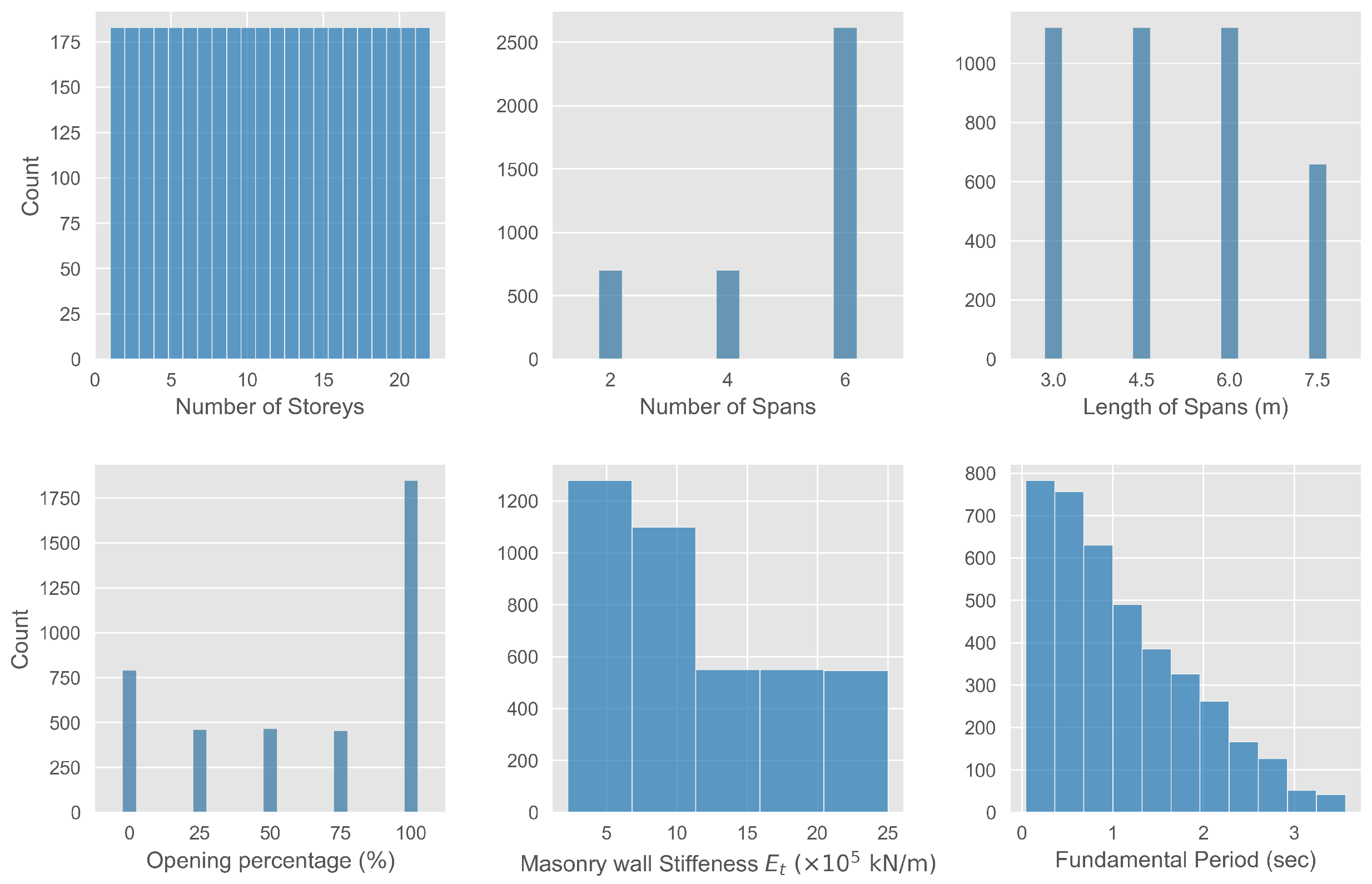
Figure 2.
Normalized SHAP values as in Equation (5).
Figure 2.
Normalized SHAP values as in Equation (5).
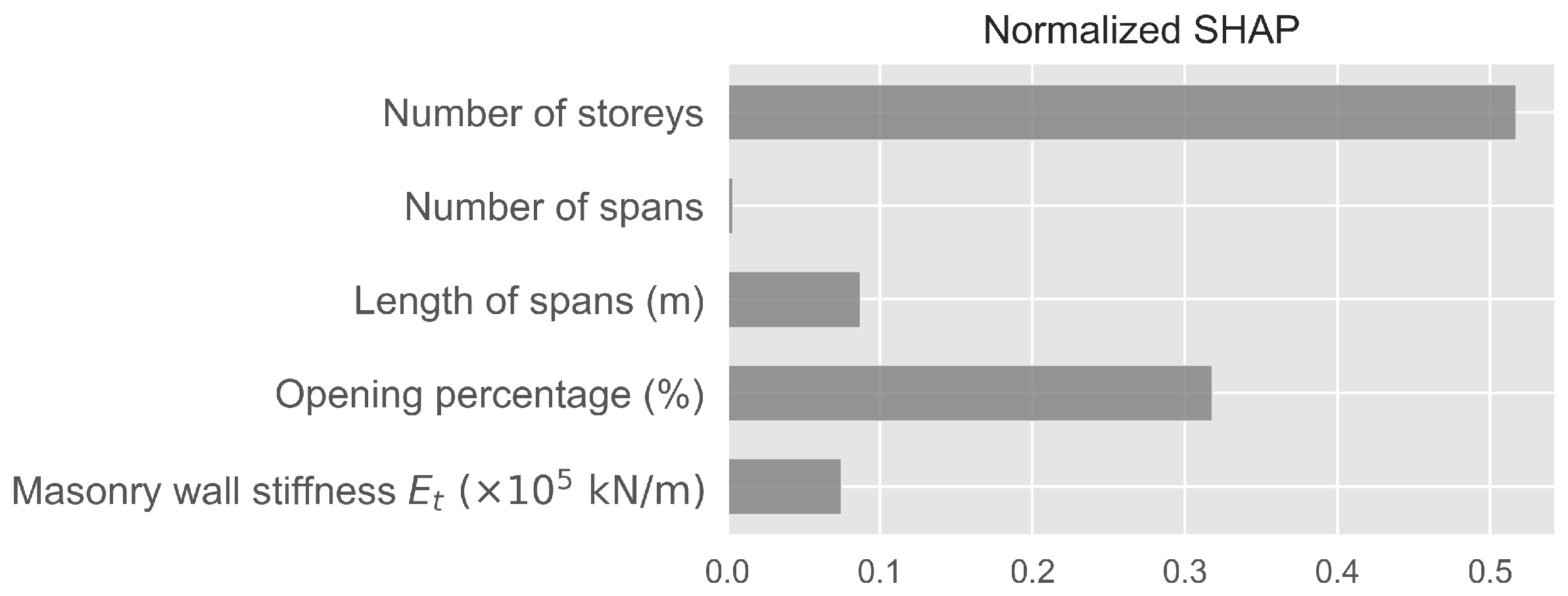
Figure 3.
Scatterplots of the SHAP values of the top two features compared with the corresponding plots of the log-transformed fundamental period.
Figure 3.
Scatterplots of the SHAP values of the top two features compared with the corresponding plots of the log-transformed fundamental period.
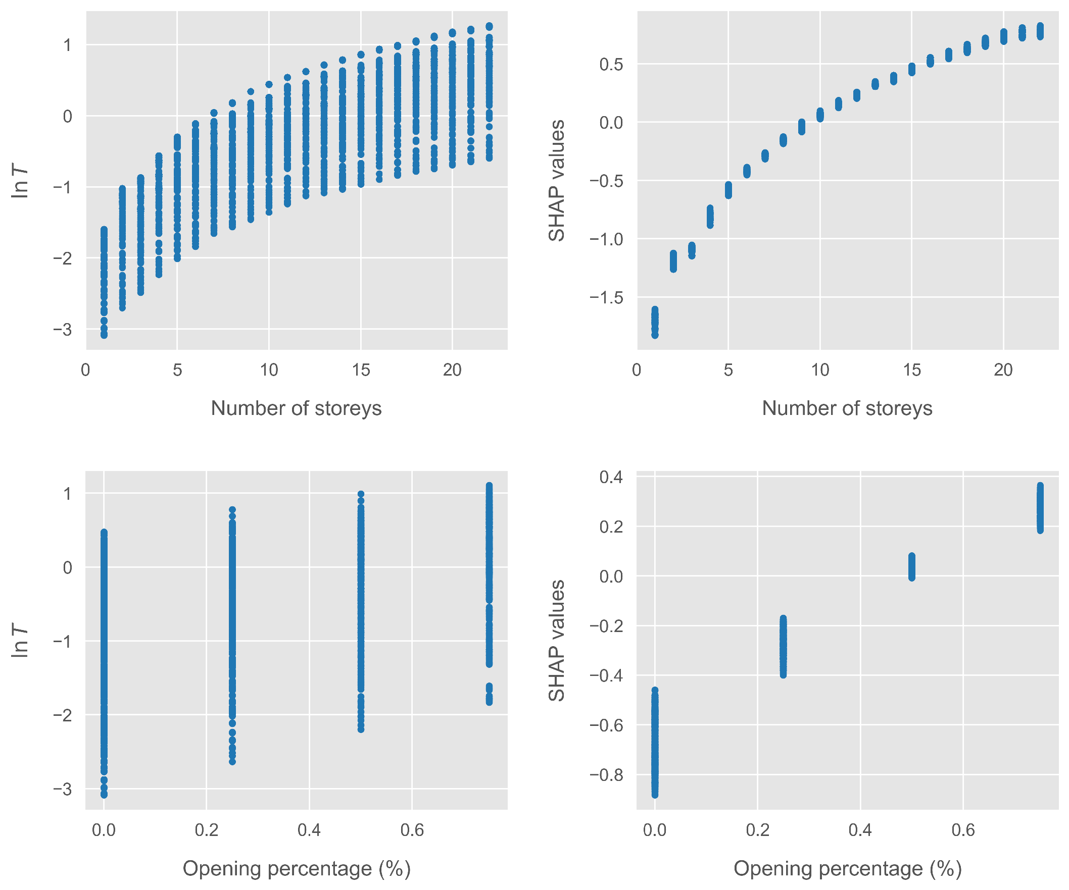
Figure 4.
Best fitted analytical curve for each feature.
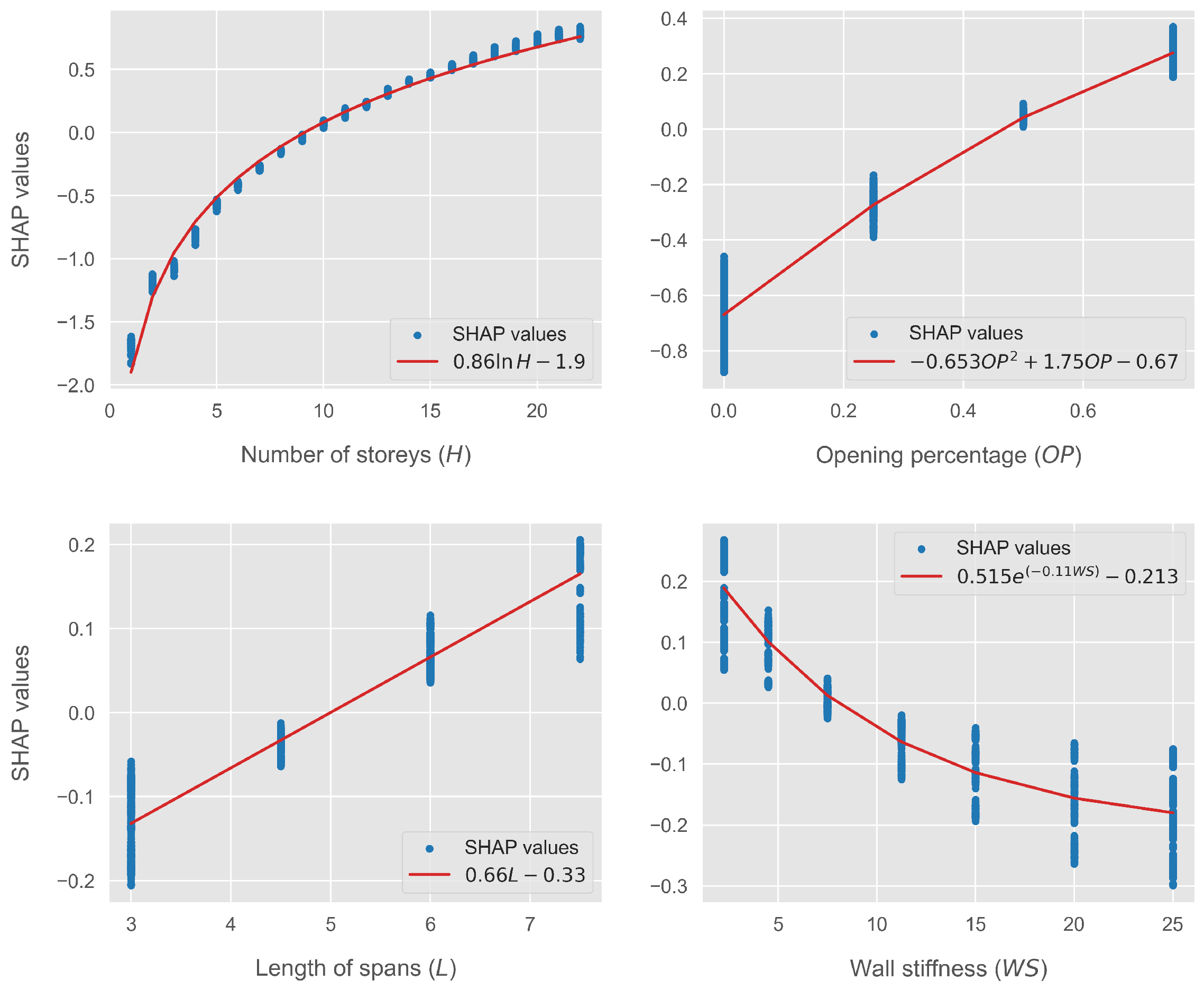
Table 3.
Fitted curves on the SHAP values of each feature. The provided equations for opening percentage and wall stiffness are valid for non-bare frames.
Table 3.
Fitted curves on the SHAP values of each feature. The provided equations for opening percentage and wall stiffness are valid for non-bare frames.
| MAE | RMSE | ||||
|---|---|---|---|---|---|
| Feature | Fitted curve | Training | Test | Training | Test |
| Number of storeys | 0.0593 | 0.0623 | 0.0763 | 0.0801 | |
| 0.0823 | 0.0837 | 0.1011 | 0.1045 | ||
| 0.0546 | 0.0575 | 0.0740 | 0.0797 | ||
| Opening percentage | 0.0758 | 0.0778 | 0.0888 | 0.0914 | |
| 0.0725 | 0.0763 | 0.0916 | 0.0955 | ||
| Length of spans | 0.0246 | 0.0308 | 0.0330 | 0.0441 | |
| 0.0358 | 0.0350 | 0.0420 | 0.0414 | ||
| Wall stiffness | 0.0450 | 0.0439 | 0.0544 | 0.0533 | |
| 0.0431 | 0.0438 | 0.0535 | 0.0538 | ||
Disclaimer/Publisher’s Note: The statements, opinions and data contained in all publications are solely those of the individual author(s) and contributor(s) and not of MDPI and/or the editor(s). MDPI and/or the editor(s) disclaim responsibility for any injury to people or property resulting from any ideas, methods, instructions or products referred to in the content. |
© 2024 by the authors. Licensee MDPI, Basel, Switzerland. This article is an open access article distributed under the terms and conditions of the Creative Commons Attribution (CC BY) license (http://creativecommons.org/licenses/by/4.0/).
Copyright: This open access article is published under a Creative Commons CC BY 4.0 license, which permit the free download, distribution, and reuse, provided that the author and preprint are cited in any reuse.


