Understanding Sorghum Farmer Typology in Sudan: A Data-Driven Lens to Scrutinize Agriculture and Rural Development

1. Introduction

Sorghum is the world’s fifth most important cereal crop grown – mostly in Central America, South Asia, and Africa where we find a quarter of world's sorghum production [1,2] and where it is used for food, fodder, and beverages. Sorghum is also widely grown across Sub-Saharan’s semi-arid regions, particularly the Sahel. In Africa, its cultivation spans from the West (Nigeria, Senegal, and Niger) to the broader East (Ethiopia and Somalia), as well as in the southern region (Zimbabwe). Besides the latter, Sudan is one of the most important countries producing sorghum in the world, ranking fifth (after China, India, USA, Nigeria, and Ethiopia) and topping the list of countries with the highest per capita in term of sorghum grain’s human consumption [3,4]. Sorghum is produced along the three sub-sectors in Sudan, namely, the irrigated, mechanized, and traditional rain-fed subsectors. The traditional rain-fed sub-sector is mainly found in Kordofan, Darfur, plus a large area in the Central States [5,6]. Moreover, the extent of its potential merits happened to differ, based on farmers’ socioeconomic diversity and locations as crucial determinants by way of boosting output, improving food security, as well as enhancing income, agriculture, and rural development [5,7,8]. In this vein, farmers are exposed to a range of both opportunities and constraints that deeply influence their prospects in terms of practice, performance, and progress. It’s worth noting that the said constraints and advantages are neither uniformly distributed nor identical among farmers, given that each category of farmers has specific resources, capabilities, and strategies [9].

In this context, a major issue arises when designing public policies with potential to generate sustainable change in agricultural systems. Numerous studies have shown that interventions’ efficiency largely depends on their ability to draw on detailed knowledge of farmer profiles, their constraints, and adaptation trajectories [8,10]. Conversely, the failure to consider this diversity has often led to the failure of agricultural policies due to their uniform and decontextualized nature [11]. Drawing up farmer typologies thus appears as an essential cornerstone for a thorough analytical approach towards understanding the complexity of agricultural systems and more effectively guiding intended interventions. By grouping sorghum farmers based on their characteristics, typology provides a framework for understanding the differentiated behaviors and farmers’ status in the face of constraints and opportunities that arise. It constitutes a solid empirical basis for designing targeted policies adapted to their agricultural systems’ diversity. Therefore, integrating the typological approach into development strategies enables decision-makers to better capture and value the farmers’ diversity, which stands as an essential condition for the sustainable and inclusive transformation of the agricultural sector.

Worldwide, research dedicated to the farming systems’ typology attempted to address this challenge by proposing classifications that allow to group farms based on their structural, functional, and socio-economic characteristics [12,13,14,15]. However, related works exhibit notable divergences: the grouping objectives vary according to studies, the classification methods difference (PCA, mixed factorial analysis, participatory approach, etc.), and the choice of variables remains highly context dependent. Moreover, typologies evolve over time, reflecting the dynamics of the farming systems per sector. These divergences explain why the construction of agricultural typologies continues to fuel scientific and methodological debate. The literature on farm typologies reveals a plurality of factors explaining the differentiation between farmers or agricultural holdings (Priegnitz et al., 2019a). Identified through empirical analyses conducted in various contexts, these factors can be divided into seven main categories: farms’ structural characteristics, economic and productive factors, households sociodemographic characteristics, conditions of access to agricultural resources and services, spatial and environmental characteristics, agricultural strategies and behaviors, as well as constraints and vulnerabilities [12].

Recent conflicts in Sudan have disrupted farming activities, lowered crop yields, food insecurity and displaced many farmers. However, innovations like drought-resistant sorghum and mobile technologies provide promising solutions. Efforts by the government and international partners focus on modernizing agriculture through improved irrigation, soil conservation, and export promotion. The country hosts a great variety of farms, the latter differing not only in their resources but also in their production strategies and adaptation methods. In this context, this ecological diversity is coupled with marked economic and social contrasts, whereby some households own and operate large, mechanized areas, while others practice subsistence farming on small plots [17]. Unequal access to inputs, markets, and infrastructure further widens these gaps. It therefore stems that one-size-fits-all agricultural policies quickly show their limitations, as they do not consider local realities or the varying/diverse farmers’ profiles. Furthermore, some researches carried out in Sudan laid specific emphasis on sorghum agriculture practices and food security [5,7]. These include: Sorghum as a potential for food security in rural areas by adaptation of technology and innovation in Sudan [18], Sorghum performance under climate change in Sudan [19], and Sorghum in food security [18,20]. However – as highlighted by some scholars [21] and [1] –, there is a scarcity of studies that focused on socioeconomic factors affecting sorghum productivity and food security also heeding farmers’ diversity, which points to the need for curb such a gap. Hence, this research attempted to fill the identified gap – at best – by providing knowledge on understanding Sorghum Farmer typology within food security in Sudan as an important factor of agriculture and Rural development.

The study suggests that socioeconomic diversity among Sudanese sorghum producers may be linked to their food security status. This is why a typological approach proves essential to understand how Sudanese agricultural households differ, what strategies they develop to cope with challenges, and how these differences can provide guidance in designing an effective policy mostly for farmers involved in sorghum production to enhance food security, resilience, and sustainability of Sudan's agriculture. In this perspective, the main objective of this study is to develop a typology of Sudanese farmers to better understand the diversity of their profiles and production strategies. Thus, the study wants to identify the socioeconomic factors that categorize the main type of sorghum producers within their food security status and analyze the correlation between farmers’ socioeconomic characteristics and the probability of belonging to a specific farmer typology prior to cluster analyses using multinomial regression. This typology aims to provide a clear reading of the country's agricultural structure and to highlight the disparities among farmers in sorghum production within their food security level. Following the Introduction section, the next one outlines the methods, the third section reports the results of the data analysis, the fourth section discusses the study’s conclusions, while the final sections are devoted to theoretical, empirical contribution of the paper within its limit, implications and the paper’s conclusions and recommendations.

2. Materials and Methods

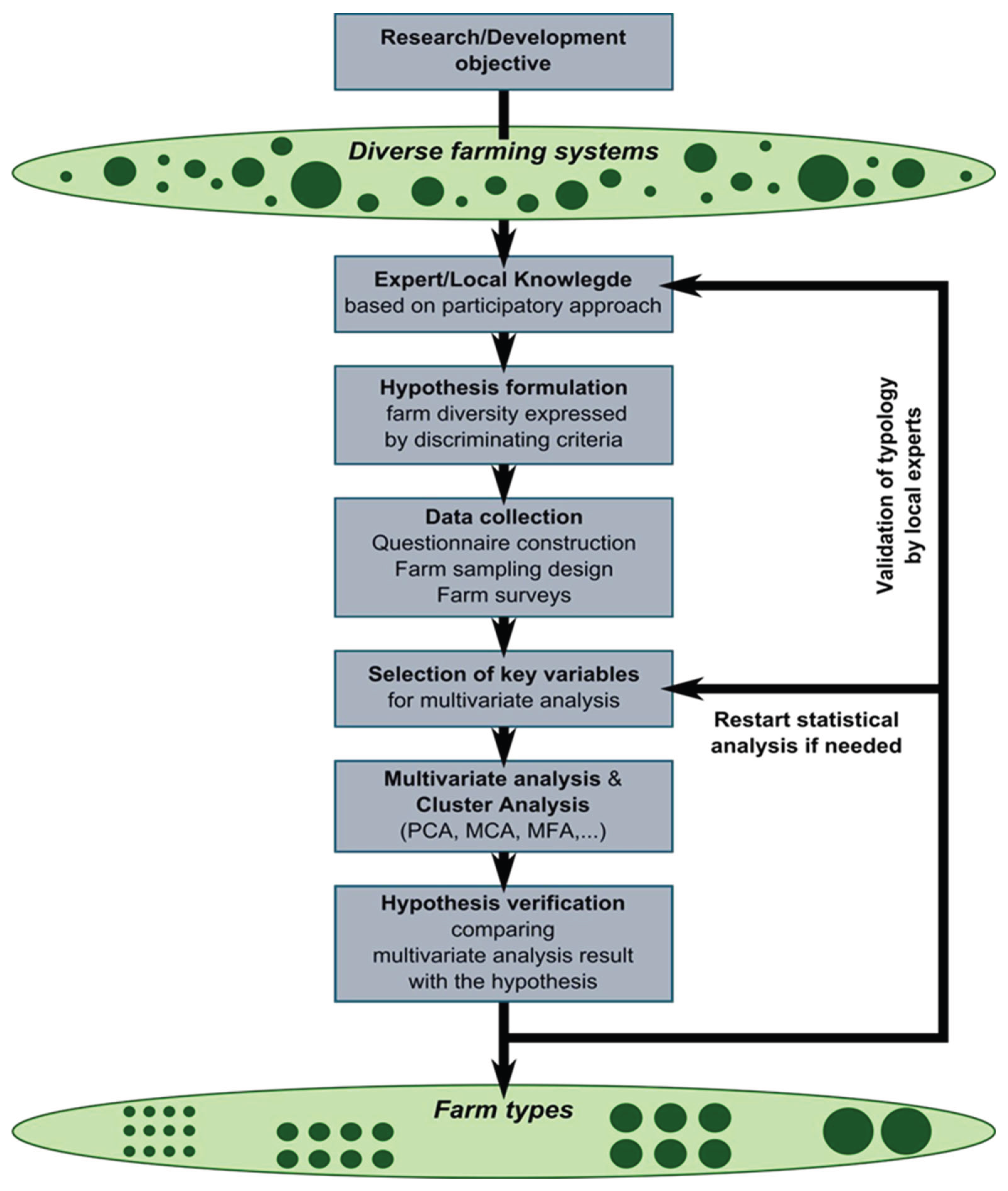
2.1. Theoretical Analytic Concept of Farmer Typology

This section outlines the approach used in this study for developing farmer typologies’ analysis. Since typologies are designed to provide answers to research questions requiring consideration of agricultural heterogeneity, they serve four primary functions: targeting suitable interventions per farm type, scaling out successful practices, selecting representative or prototype farms for deeper analysis, and scaling up ex-ante impact assessments to broader regions [5,7]. In the humid tropics and in semi-arid regions of Sub-Saharan Africa, farming systems span a wide array of landscapes and cultures, shaped by diverse biophysical, economic, and institutional conditions that differ significantly across regions and even within themselves [16,22]. This variation leads to distinct development stages among farms, shaped by farmers’ differing skill sets, aspirations, and resource access, all of which generate dynamic spatial and temporal heterogeneity. Such complexity is difficult to fully capture, often resulting in partial representations of the real situation. To address this, various tools – such as wealth rankings, typologies, and farm classifications – have been developed, each balancing the trade-off between detailed representation and practical usability [23,24,25].

Several methods are available for constructing typologies, including comparative analyses of farm functioning, expert-based clustering, participatory wealth rankings, and multivariate statistical techniques like Principal component analysis (PCA) or Multiple Correspondence Analysis (MCA). While expert knowledge methods are cost-effective and context-sensitive, statistical approaches are often preferred for their reproducibility and objectivity; ideally, both approaches are combined for robust results [10]. Typology construction must meet scientific standards of accuracy and reproducibility, while also addressing stakeholder needs [10,17]. The process goes through six key steps (Figure 1) that respectively consist of: defining objectives, hypothesizing diversity, choosing relevant variables, designing sampling, applying clustering, and validating using local knowledge. Given that farms evolve over time, typologies – based on one-time data – should be regularly revised to remain useful. In data-limited contexts, and for this study, structural typologies based on resource endowments offer a viable starting point as suggested by previous studies [15,26]. Hypothesis was formulated on expected effect of sorghum farmers’ diversity on their food security, and collaboration with local stakeholders was developed, informed by expert input. Furthermore, field observations and survey were conducted, previous research on Sudanese farmers on different socioeconomic and demographics aspects within sorghum production were consulted, ensuring that the typology aligns with both theoretical insights and local real context.

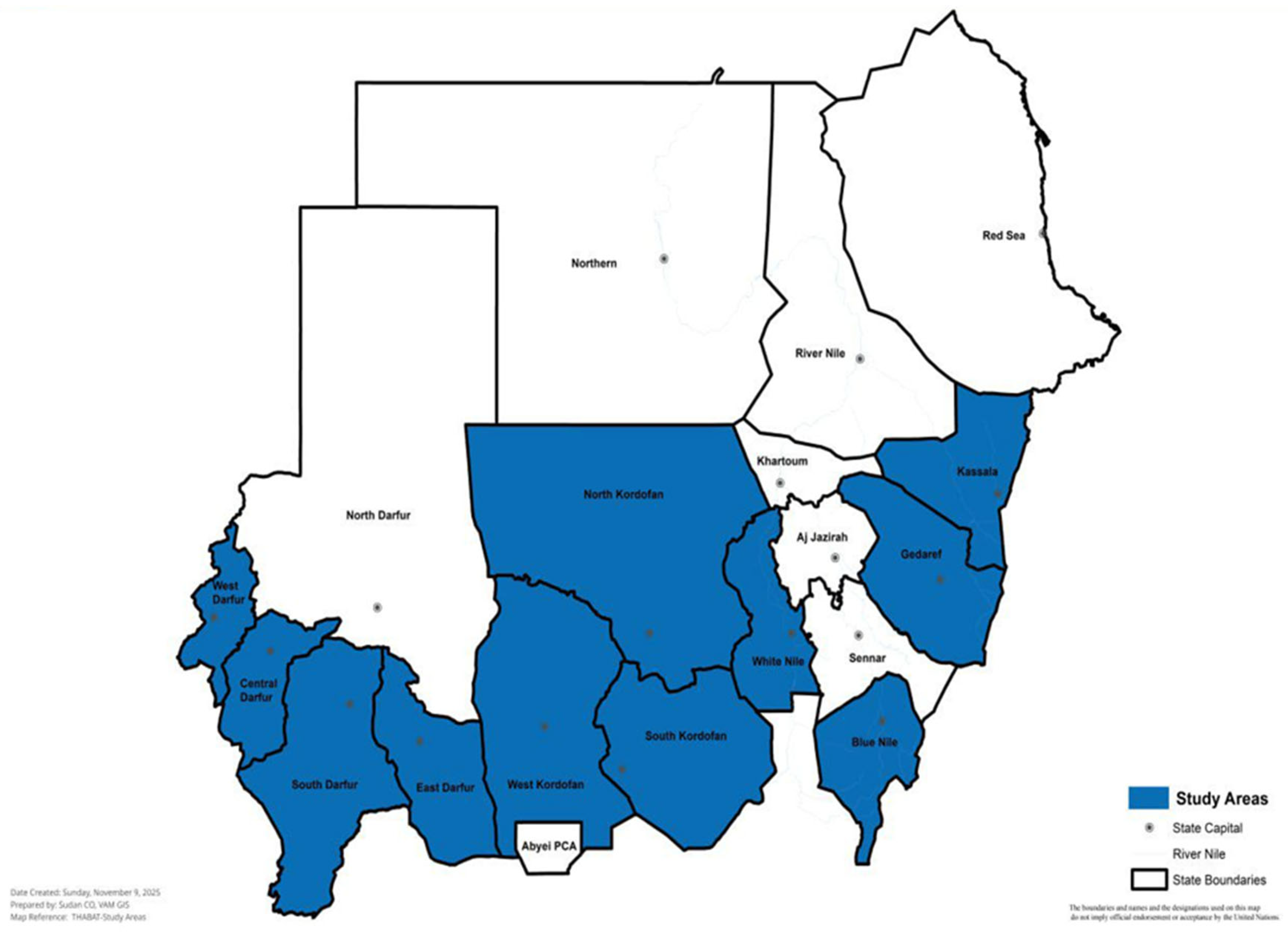
2.2. Study Areas and Sample

Commonly known as “the grain of the Tropics,” sorghum is a cornerstone of Sudan’s agriculture, food security, and rural economy. As one of Africa’s leading producers, Sudan relies heavily on sorghum as a staple food, mostly in rural areas where it forms the backbone of livelihoods [7]. In Sudan, between the northern semi-arid zones, the Central region’s savannas, and the irrigated plains in the South, sorghum thrives across Sudan’s diverse agro-ecological zones where it has been cultivated for centuries, with Gadarif State alone accounting for over 60% of the country’s production due to its dominance in mechanized agriculture [29]. Other key regions include the Blue Nile, Kordofan, and Darfur, where both traditional and mechanized methods are used. Farmers have started diversifying with crops like millet and sesame to mitigate these risks [18,29,30].

The sorghum farming calendar begins with sowing in June and harvesting in November, but productivity is hindered by outdated machinery, poor access to seeds, low fertilizer use, and inadequate storage infrastructure. Many farmers lack access to financial services and modern farming knowledge [5]. Agricultural cooperatives are increasingly playing a role in bridging these gaps, offering shared resources, improved tools, and market access. Economics wise, sorghum contributes significantly to Sudan’s GDP and rural employment, supporting over 1.5 million households [5,6]. Annual production exceeds 4.5 million metric tons, with exports – primarily to Saudi Arabia and Yemen – bringing in around $200 million in 2022 [29]. However, export growth is constrained by poor infrastructure, lack of processing facilities, and limited foreign investment.

Armed conflict has disrupted sorghum production in Sudan by displacing farmers and reducing yields. Yet, innovations such as climate-resilient crop varieties and mobile platforms offer a path forward. Government and international efforts are underway to modernize agriculture via irrigation upgrades, soil restoration, and export incentives [18,30,31]. This study is based on data from a quantitative survey conducted in 2022, involving 392 farmer households in several States (Figure 2) of Sudan, namely Blue Nile, Central Darfur, East Darfur, Gedarif, Kassala, North Kordofan, South Darfur, South Kordofan, West Darfur, West Kordofan, and White Nile. The sampling design was designed according to geographical and socio-economic stratification to ensure the representativeness of different agricultural systems. Households were selected randomly. The survey questionnaire was administered on a face-to-face basis by trained interviewers. It covered sociodemographic characteristics of the household heads; productive and land resources; household income and expenditure; as well as conditions of access and infrastructure (distances to markets, agricultural services, and main roads).

2.3. Empirical Model of PCA

PCA is a multivariate statistical technique used to reduce the number of variables in a data set into a smaller number of ‘dimensions [32,33,34]. In mathematical terms, from an initial set of correlated variables, PCA creates uncorrelated indices or components, where each component is a linear weighted combination of the initial variables. For example, from a set of variables X1 through to Xn,

$${PC}_1=a_{11}{X}_1+a_{11}{X}_1+\text{…}{a}_{1n}{X}_n$$

(1)

$${PC}_m=a_{m1}{X}_1+a_{m2}{X}_2 \text{…}.+a_{mn}{X}_n$$

(2)

where $a_{mn}$represents the weight for the $m$ th principal component and $n$ th variable. Diagrammatically, the weights for each principal component are given by the eigenvectors of the correlation matrix, or if the original data were standardized. The variance ($\lambda$) for each principal component is given by the eigenvalue of the corresponding eigenvector. The components are arranged in such a manner that the first component (PC1) explains the largest possible amount of variation in the original data, subject to the constraint that the sum of the squared weights ($a_{11}^2+a_{12}^2$ + $a_{1n}^2$) is equal to one. As the sum of the eigenvalues equals the number of variables in the initial data set, the proportion of the total variation in the original data set accounted by each principal component is given by ${\displaystyle \raisebox{1ex}{$\lambda $}\!\left/ \!\raisebox{-1ex}{$n$}\right.}$. The second component (PC2) is completely uncorrelated with the first component and explains additional – yet lesser – variation than the first component, subject to the very same constraint. Subsequent components are uncorrelated with previous components; therefore, each component captures an additional dimension in the data, while explaining smaller proportions of the variation of the original variables. The higher the degree of correlation among the original variables in the data, the fewer components required to capture common information.

2.3. Multinomial Logistic Regression

A multinomial logistic regression model was applied to analyze the relationship between household socioeconomic, demographic characteristics and the probability of belonging to a specific farmer type. The approach is in line with [35] study. Derived from prior clustering analyses, the typologies represent mutually exclusive and collectively exhaustive categories, justifying the use of a multinomial specification for categorical outcomes with more than two levels. The model estimates the log-odds of each typology relative to a reference category [25,36]. Typology “B” representing the household type. Formally, for each non-reference category $k$, the model is specified as:

$$\mathrm{l}\mathrm{o}\mathrm{g}\left({\displaystyle \frac{P(Y=k)}{P(Y=B)}}\right)={\beta }_{0k}+{\beta }_{1k}{X}_1+{\beta }_{2k}{X}_2+\cdots +{\beta }_{pk}{X}_p$$

(3)

where $Y$ denotes the farmer typology, and $X_1,X_2,\dots ,X_p$ represent household- and farm-level explanatory variables [37]. These include household size, age, and education of the household head, land size, income sources, expenditures, Tropical Livestock Unit (TLU), and food security indicators such as the Household Food Insecurity Access Scale (HFIAS) and the Household Dietary Diversity Score (HDDS).

The parameters ${\beta }_{0k}$ and ${\beta }_{ik}$ represent the intercept and slope coefficients for category $k$, respectively. Coefficients were estimated through Maximum Likelihood Estimation (MLE). For interpretability, coefficients were exponentiated to yield odds ratios, indicating the multiplicative change in the odds of belonging to a typology $k$ [35,36,37]. The multinomial logistic framework allows for the simultaneous assessment of multiple socio-economic and agricultural determinants across typologies. This approach is particularly suited to identifying key differentiating characteristics among heterogeneous farmer groups, thereby providing an empirical basis for targeted agricultural policies and livelihood-oriented interventions.

2.4. Variables and Related Measurements

The choice of variables, as illustrated in Table 1, was based on existing literature on farm household typology [11,14]. Structural characteristics constitute the first set of criteria used in agricultural typologies [17]. They majorly include land size, number of plots, ownership of agricultural equipment, and livestock, which reflect the productive capacity and level of physical capital of farmers. Economic and productive factors, on the other hand, refer to agricultural and non-agricultural incomes, expenditures, and productivity, highlighting the disparities in performance and orientation between subsistence and commercial farms [38]. The sociodemographic characteristics of farmers, such as age, education level, household size, and agricultural experience, influence production decisions, innovation capacity, and resource management [11]. Conditions of access to finance resources and services include variables related to labor availability, which determine the adoption of new technologies and farm competitiveness [25,39]. Furthermore, spatial and environmental characteristics, including distance to markets, and to the urban area explain regional differences in productivity and economic integration [40]. Agricultural production strategies and behaviors, such as sorghum land size, total land size, reflect the economic and adaptive choices of households. Lastly, constraints and vulnerabilities, whether cost of land rental, food security status, and livestock ownership reflect the differentiated resilience of farms to shocks and constitute a major determinant of agricultural system transformations. Owing to its vastness and diverse environmental patterns, Sudan exemplifies a model particularly exhibiting a typical illustration of the complexity of African agricultural systems [8,17,23].

2.5. Data Analysis

In this study, two multivariate analysis techniques – namely Principal Component Analysis (PCA) and cluster analysis – were used to establish a typology of farmer households in Sudan. The two methods have been widely used by several studies to characterize and differentiate agricultural systems according to their specificities [13,15,24]. First, a Principal Component Analysis (PCA) was performed in R-Studio [41] on a set of variables relating to the sociodemographic characteristics of households, conditions of access to the urban market, agricultural assets, agriculture production strategy and the economic features of households (expenditure and income). The objective was to summarize the complexity of the data and identify the dimensions that structure the diversity of agricultural households. The factorial axes were selected based on the Kaiser criterion (eigenvalues > 1) and the scree plot. Only factorial axes with eigenvalues greater than 1 were retained. Additionally, the Kaiser-Meyer-Olkin (KMO) measure for sampling adequacy should generate a value greater than 0.5 and the Bartlett's sphericity test, with an associated p-value less than 0.001, to indicate the validity of the analysis. Afterwards, a hierarchical cluster analysis was performed using the identified principal components. The cluster analysis made it possible to group the observations based on extent of their similarity measured across all captured dimensions. This type of analysis helps identify homogeneous groups of farmer households that share similar features while maximizing the differences between the formed groups. A multinomial logistic regression model was performed in Stata 17 [42] to analyze the relationship between household and farm-level characteristics and the probability of belonging to a specific farmer type. Hence, statistical significance was assessed using z-values and p-values.

3. Results

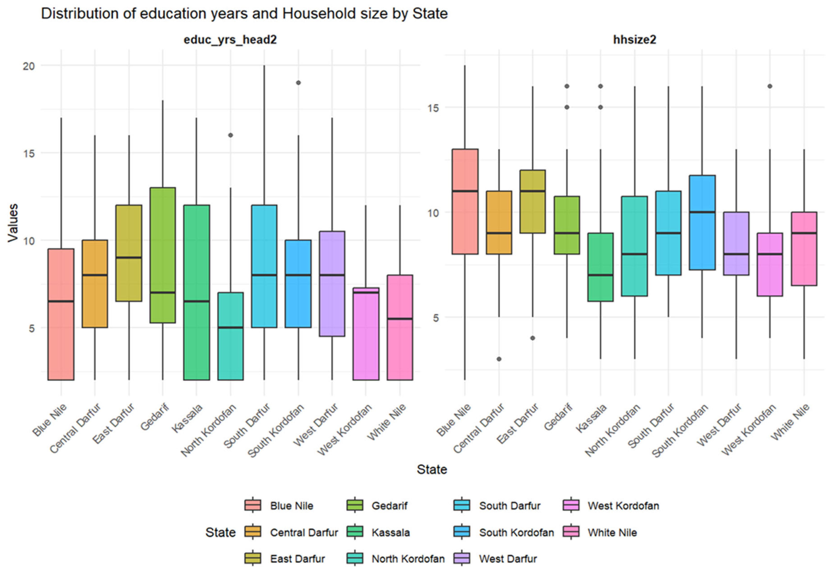
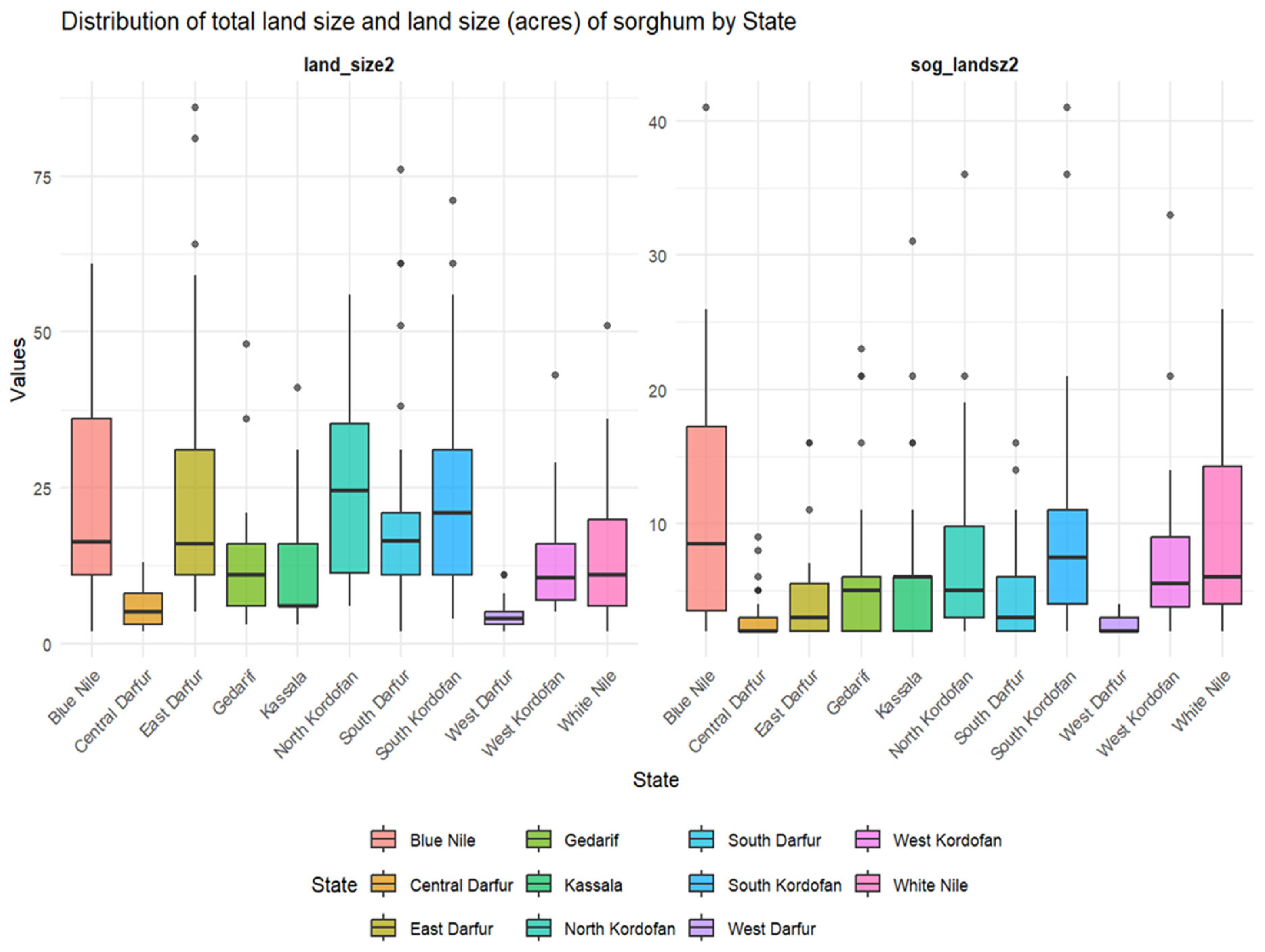
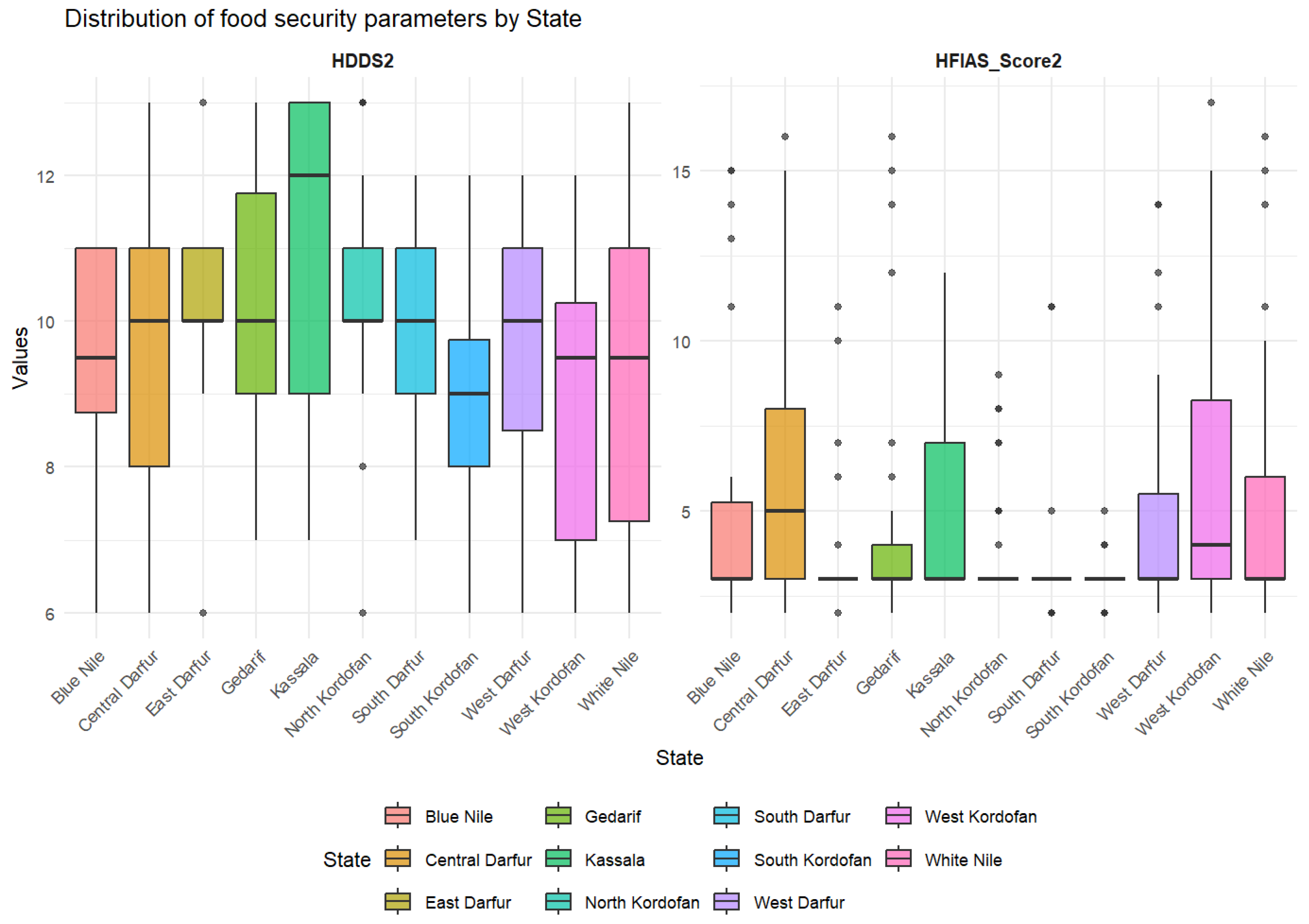
3.1. Cross-States’s Descriptive Statistics

The results show significant variation across States in almost all households and farm characteristics, as confirmed by the p-values (mostly <0.01), indicating meaningful regional disparities in socio-economic and agricultural conditions across Sudan. Average household size differs significantly (p = 0.000), ranging from 7.6 in Kassala to 10.8 in Blue Nile, reflecting different family structures and dependency ratios. Although the average age of the household head does not differ significantly (p = 0.167), the trend shows older heads in North Kordofan (54 years) and younger ones in Blue Nile (44 years), suggesting possible migration and generational differences in leadership patterns. Education levels also vary markedly (p = 0.000), with higher schooling years in Gedarif (9.4) and East Darfur (9.4) compared to only 5.4 in North Kordofan, revealing regional inequalities in access to education and human capital formation. Accessibility variables such as distance to farmland and to towns exhibit strong regional contrasts (p = 0.000); households in North Kordofan and Central Darfur are located closer to fields and markets, whereas East Darfur and Blue Nile face longer distances (above 100 and 67 minutes, respectively). Economic and income variables show substantial divergence (all p < 0.01), with Gedarif and Kassala reporting the highest total and food expenditures, indicating more commercialized, market-linked economies, while North Kordofan and Blue Nile exhibit lower incomes and expenditures, aligning with subsistence-oriented production systems. Off-farm income is notably higher in East Darfur and Gedarif, suggesting diversification of livelihoods outside farming. Landholding size also differs significantly (p = 0.000), with Gedarif (26.6 feddans) and Blue Nile (23.9 feddans) having the largest average holdings and Central Darfur the smallest (5.9 feddans), reflecting the predominance of smallholder systems in the Darfur region compared to semi-mechanized farming in the east. Similarly, labor hiring costs vary widely (p = 0.000), peaking in Gedarif (228,840 SDG) due to the prevalence of commercial agriculture, but minimal in Central Darfur (623 SDG), emphasizing structural differences in farm mechanization and labor intensity. Food security indicators display equally sharp contrasts (p = 0.000): dietary diversity (HDDS) is highest in North Kordofan (11.0) and East Darfur (10.2) but lowest in Blue Nile (9.3), while food insecurity (HFIAS) peaks in Central Darfur (6.3) and is lowest in East Darfur (3.8), revealing uneven access to food and nutritional diversity. Livestock holdings, measured through chicken ownership (p = 0.007), are relatively similar but slightly lower in North Kordofan, while land rent costs are highest in Kassala and Central Darfur, likely due to competition over limited cultivable land. Overall, the results highlight pronounced spatial heterogeneity among Sudanese States: the eastern States (Gedarif, Kassala) exhibit higher income, education, and land ownership associated with commercial agriculture; the western States (Darfur region) remain land- and resource-constrained with lower incomes and greater food insecurity, while Blue Nile lies in an intermediate position with large households and moderate land access but high isolation and dietary limitations. These patterns underline the need for geographically tailored interventions that strengthen market access, promote equitable education, enhance agricultural productivity, and address the specific challenges to resilience and food security in each of the involved States.

Table 2. Cross-States’ Descriptive Statistics.

Variables/States	Blue Nile (N=28)	Central Darfur (N=41)	East Darfur (N=27)	Gedarif (N=38)	Kassala (N=36)	North Kordofan (N=38)	P-value
hhsize2	10.75 (4.05)	9.15 (2.45)	10.44 (3.00)	9.13 (2.517)	7.639 (3.01)	8.55 (3.32)	0.000
age_head2	43.79 (10.30)	47.54 (12.50)	49.96 (10.63)	49.42 (11.693)	54.139 (12.01)	48.18 (14.35)	0.167
educ_yrs_head2	6.79 (4.49)	7.59 (3.95)	9.41 (4.13)	9.26 (4.914)	7.083 (5.00)	5.39 (3.91)	0.000
dist_mins2	67.11 (43.92)	26.59 (32.29)	104.89 (24.59)	43.03 (33.837)	21.889 (26.98)	66.66 (42.41)	0.000
dist_town2	41.54 (26.75)	8.24 (9.88)	73.48 (21.10)	21.79 (20.98)	50.917 (30.18)	39.18 (22.49)	0.000
annual_nonAgrInc2	346,038.44 (390,794.05)	365,338.43 (311,799.30)	528,297.47 (429,543.46)	427,719.41 (508,879.391)	183,744.018 (210,204.79)	425,385.77 (416,092.69)	0.002
annual_Income2	419,286.71 (412,126.88)	395,412.59 (315,291.23)	645,350.33 (524,869.78)	528,101.87 (523,697.576)	282,142.172 (318,704.49)	569,124.68 (383,581.32)	0.000
annual_hhd_exp2	550,802.43 (288,538.51)	619,250.56 (353,319.97)	1,321,342.93 (605,248.01)	1,251,717.63 (566,672.480)	921,200.11 (506,237.29)	919,954.68 (450,956.41)	0.000
annual_food_exp2	378,373.86 (257,681.56)	397,338.56 (210,200.39)	893,689.89 (405,823.69)	870,417.36 (445,687.607)	676,749.33 (403,538.94)	632,565.21 (346,476.56)	0.000
annual_exp_nonfd2	172,429.57 (105,687.25)	221,913.00 (209,574.79)	427,654.04 (246,744.54)	396,802.89 (226,577.384)	244,451.778 (190,432.59)	287,390.47 (189,142.34)	0.000
land_size2	23.87 (18.96)	5.90 (3.25)	26.57 (22.57)	12.34 (8.936)	11.056 (9.17)	24.71 (14.42)	0.000
sog_landsz2	11.18 (9.68)	3.00 (1.67)	4.63 (3.95)	6.13 (5.639)	6.389 (6.10)	7.79 (7.37)	0.000
labhire_totcost2	29,686.62 (131,813.61)	623.00 (0.00)	3,480.52 (11,296.56)	228,839.81 (105,158.25)	1,333.88 (6,114.84)	14,713.96 (38,553.45)	0.000
HDDS2	9.29 (1.67)	9.41 (1.79)	10.22 (1.25)	10.03 (1.952)	11.000 (1.93)	10.34 (1.36)	0.000
HFIAS_Score2	5.21 (4.16)	6.29 (4.03)	3.81 (2.17)	4.47 (3.57)	4.972 (2.58)	3.82 (1.69)	0.000
unitcst_landrent2	3,861.08 (2,871.59)	9,352.69 (11,940.74)	8,397.42 (11,506.6)	9,894.66 (14,904.29)	5,268.6 (5,159.33)	5,397.56 (5,847.83)	0.000
chicken_qnty_tlu2	2.05 (0.07)	2.08 (0.37)	2.06 (0.08)	2.01 (0.193)	2.070 (0.20)	1.90 (0.26)	0.007

Table 2. Cross-States’ Descriptive Statistics.

Variables/States	Blue Nile (N=28)	Central Darfur (N=41)	East Darfur (N=27)	Gedarif (N=38)	Kassala (N=36)	North Kordofan (N=38)	P-value
hhsize2	10.75 (4.05)	9.15 (2.45)	10.44 (3.00)	9.13 (2.517)	7.639 (3.01)	8.55 (3.32)	0.000
age_head2	43.79 (10.30)	47.54 (12.50)	49.96 (10.63)	49.42 (11.693)	54.139 (12.01)	48.18 (14.35)	0.167
educ_yrs_head2	6.79 (4.49)	7.59 (3.95)	9.41 (4.13)	9.26 (4.914)	7.083 (5.00)	5.39 (3.91)	0.000
dist_mins2	67.11 (43.92)	26.59 (32.29)	104.89 (24.59)	43.03 (33.837)	21.889 (26.98)	66.66 (42.41)	0.000
dist_town2	41.54 (26.75)	8.24 (9.88)	73.48 (21.10)	21.79 (20.98)	50.917 (30.18)	39.18 (22.49)	0.000
annual_nonAgrInc2	346,038.44 (390,794.05)	365,338.43 (311,799.30)	528,297.47 (429,543.46)	427,719.41 (508,879.391)	183,744.018 (210,204.79)	425,385.77 (416,092.69)	0.002
annual_Income2	419,286.71 (412,126.88)	395,412.59 (315,291.23)	645,350.33 (524,869.78)	528,101.87 (523,697.576)	282,142.172 (318,704.49)	569,124.68 (383,581.32)	0.000
annual_hhd_exp2	550,802.43 (288,538.51)	619,250.56 (353,319.97)	1,321,342.93 (605,248.01)	1,251,717.63 (566,672.480)	921,200.11 (506,237.29)	919,954.68 (450,956.41)	0.000
annual_food_exp2	378,373.86 (257,681.56)	397,338.56 (210,200.39)	893,689.89 (405,823.69)	870,417.36 (445,687.607)	676,749.33 (403,538.94)	632,565.21 (346,476.56)	0.000
annual_exp_nonfd2	172,429.57 (105,687.25)	221,913.00 (209,574.79)	427,654.04 (246,744.54)	396,802.89 (226,577.384)	244,451.778 (190,432.59)	287,390.47 (189,142.34)	0.000
land_size2	23.87 (18.96)	5.90 (3.25)	26.57 (22.57)	12.34 (8.936)	11.056 (9.17)	24.71 (14.42)	0.000
sog_landsz2	11.18 (9.68)	3.00 (1.67)	4.63 (3.95)	6.13 (5.639)	6.389 (6.10)	7.79 (7.37)	0.000
labhire_totcost2	29,686.62 (131,813.61)	623.00 (0.00)	3,480.52 (11,296.56)	228,839.81 (105,158.25)	1,333.88 (6,114.84)	14,713.96 (38,553.45)	0.000
HDDS2	9.29 (1.67)	9.41 (1.79)	10.22 (1.25)	10.03 (1.952)	11.000 (1.93)	10.34 (1.36)	0.000
HFIAS_Score2	5.21 (4.16)	6.29 (4.03)	3.81 (2.17)	4.47 (3.57)	4.972 (2.58)	3.82 (1.69)	0.000
unitcst_landrent2	3,861.08 (2,871.59)	9,352.69 (11,940.74)	8,397.42 (11,506.6)	9,894.66 (14,904.29)	5,268.6 (5,159.33)	5,397.56 (5,847.83)	0.000
chicken_qnty_tlu2	2.05 (0.07)	2.08 (0.37)	2.06 (0.08)	2.01 (0.193)	2.070 (0.20)	1.90 (0.26)	0.007

Table 3 [Cross-States’ Descriptive Statistics (Continued)], below, presents the comparison of household and agricultural characteristics across South Darfur, South Kordofan, West Darfur, West Kordofan, and White Nile reveals marked regional heterogeneity in livelihoods and resource endowments, with most differences statistically significant (p < 0.01). Overall, average household sizes are high, ranging from 8 in West Kordofan to 10 in South Kordofan, reflecting the large family systems, typical of rural Sudan, while education levels differ significantly (p = 0.000), being highest in South Darfur (8.7 years) and lowest in White Nile (5.4 years) – denoting an uneven human capital investment across States. Accessibility indicators show that South Kordofan households live closest to farms and towns, while West Darfur and South Darfur record the longest distances, indicating location-based (distance related) constraints to market access and service delivery. Income and expenditure patterns also vary sharply (all p < 0.01): White Nile households exhibit the highest annual income (580,600 SDG) and total expenditures (814,000 SDG), while West Kordofan and West Darfur show significantly lower means, highlighting their weaker purchasing power and market integration. North and South Kordofan maintain the largest average landholdings (20–25 feddans), while West Darfur farms are the smallest (4), suggesting land fragmentation and pressure in conflict-affected zones. Similarly, sorghum land size and seasonal cultivated land follow the same trend, with South Kordofan being the most endowed land. Labor hiring costs vary greatly, standing as the highest in South Darfur (31,600 SDG), thereby reflecting relatively active commercial farming, but minimal in West Darfur and White Nile, suggesting more family-based or subsistence production. Food security indicators further reveal contrasting welfare conditions: HFIAS scores are highest in West and White Nile (5–6), implying greater food insecurity, while South Kordofan and South Darfur show relatively lower scores (3), indicating moderately better access to food. Conversely, HDDS scores are highest in South Darfur (9.9) and West Darfur (9.7) but lowest in South Kordofan (8.7), demonstrating variation in dietary diversity across States. Overall, the findings portray South Kordofan as relatively land-rich and accessible though moderately poor in dietary diversity; White Nile as income-rich but food-insecure; South Darfur as a more commercially active agricultural zone with better diet diversity; and West Darfur and West Kordofan as the most disadvantaged in both land and income, facing persistent structural and food access challenges.

Figure 4 (below) shows the education years and household size across eleven States surveyed. Each boxplot summarizes regional disparities in both education and household composition. For education years (left panel), there are notable differences across States. The length of schooling is generally concentrated between 5 and 10 years, indicating that most individuals have attained a ‘basic to lower secondary’ level of education. South Darfur stands out, exhibiting the highest educational attainment with an upper limit of 20 years of schooling, reflecting existence of highly educated individuals. In contrast, West Kordofan ranks lowest, with schooling levels not exceeding 12 years, highlighting comparatively limited educational attainment in that State. Gedarif, Kassala, and North Kordofan show relatively higher rates in terms of years of education, suggesting access to schooling or stronger emphasis on education in these regions. In contrast, Blue Nile, South Kordofan, and White Nile display lower level of education years, implying more limited educational attainment among household heads.

East Darfur stands out, with its population having 8 to 19 years of education, indicating a more advanced educational profile, like that observed in Blue Nile and South Kordofan. The Gedaref State shows a broader educational distribution, with half of the population having 5 to 16 years of schooling. In Kassala, 75% of the population has between 2 and 12 years of schooling, with the top 25% reaching 12 to 17 years, reflecting a moderate overall education level. Conversely, North Kordofan exhibits a lower educational profile. South Darfur presents the highest education ceiling, with an upper extreme of 20 years of schooling. Lastly, West Kordofan and White Nile States reflect the lowest education levels, with schooling years not exceeding 12 years among their populations. The household size plot also highlights strong regional variation, and the figure indicates that Sudanese account for high rates in terms of household fertility, with average household sizes usually ranging from 7 to 12 individuals, reflecting considerable demographic diversity across regions. Among these States, Blue Nile stands out with the largest household sizes, reaching a maximum of 17 individuals per family, which indicates particularly high population density at the household level in this area. Central Darfur, East Darfur, and South Kordofan happen to have larger households’ members, averaging 10–12 members, which may reflect extended family living arrangements or higher birth rates in these States. In contrast, Kassala and Gedarif show relatively smaller household sizes, generally between 6 and 8 members.

Figure 5 presents the distribution of total and sorghum land sizes in acres across eleven States in Sudan. Allowing for comparison of agricultural land holdings and the extent of sorghum cultivation between regions. The Figure reveals that agricultural landholdings across the Sudanese States generally range between 0 - and 37-acres significant variability in land distribution among households. In contrast, the land portion specifically dedicated to sorghum cultivation is more limited, typically ranging between 0 and 10 acres, indicating that sorghum occupies only a given portion of the total cultivated area among other crops. Blue Nile province stands out with the largest agricultural landholding, reaching up to 62 acres, with a maximum of 26 acres allocated to the crop. At the other edge of the spectrum, West Darfur has the smallest agricultural landholdings, with areas not exceeding 10 acres. Regarding total land size, substantial regional variation is observed. Blue Nile, South Kordofan, and South Darfur exhibit relatively larger land sizes, suggesting that households in these States have access to more extensive agricultural land, possibly due to favorable agroecological conditions or less demographic pressure. In contrast, Central Darfur, West Darfur, and Kassala display smaller land sizes, indicating more limited access to cultivable land.

Figure 6 presents the distribution of two key food security indicators – Household Dietary Diversity Score (HDDS) and Household Food Insecurity Access Scale (HFIAS) – across Sudan’s States. These indicators offer valuable insight into the quality of diets and the severity of food access challenges at the household level, making them reliable tools for assessing vulnerability and resilience in rural agricultural settings. The Figure reveals that most households fall within a dietary diversity range of 8 to 10 food groups, indicating a moderate but limited variety in daily food consumption. Gedaref and Kassala exhibit the highest scores. Blue Nile, Central Darfur, East Darfur, and White Nile also show relatively high median HDDS values, though their distributions are somewhat more concentrated. On the other hand, South Darfur and North Kordofan exhibit the lowest median HDDS scores, suggesting more limited dietary diversity. West Kordofan and South Kordofan display a wider spread in HDDS values, pointing to internal inequalities in food access and nutrition. The HFIAS scores, which capture perceived food insecurity, reveal a different pattern. East Darfur, South Darfur, South Kordofan, and North Kordofan report the lowest HFIAS scores, indicating relatively stable food access and lower perceived stress around food availability. In contrast, West Kordofan, White Nile, and West Darfur show significant scores and greater variability, signaling a significant proportion of households experiencing food insecurity. Central Darfur and Blue Nile fall in the middle range but show notable dispersion, possibly reflecting localized differences in access to aid or agricultural inputs.

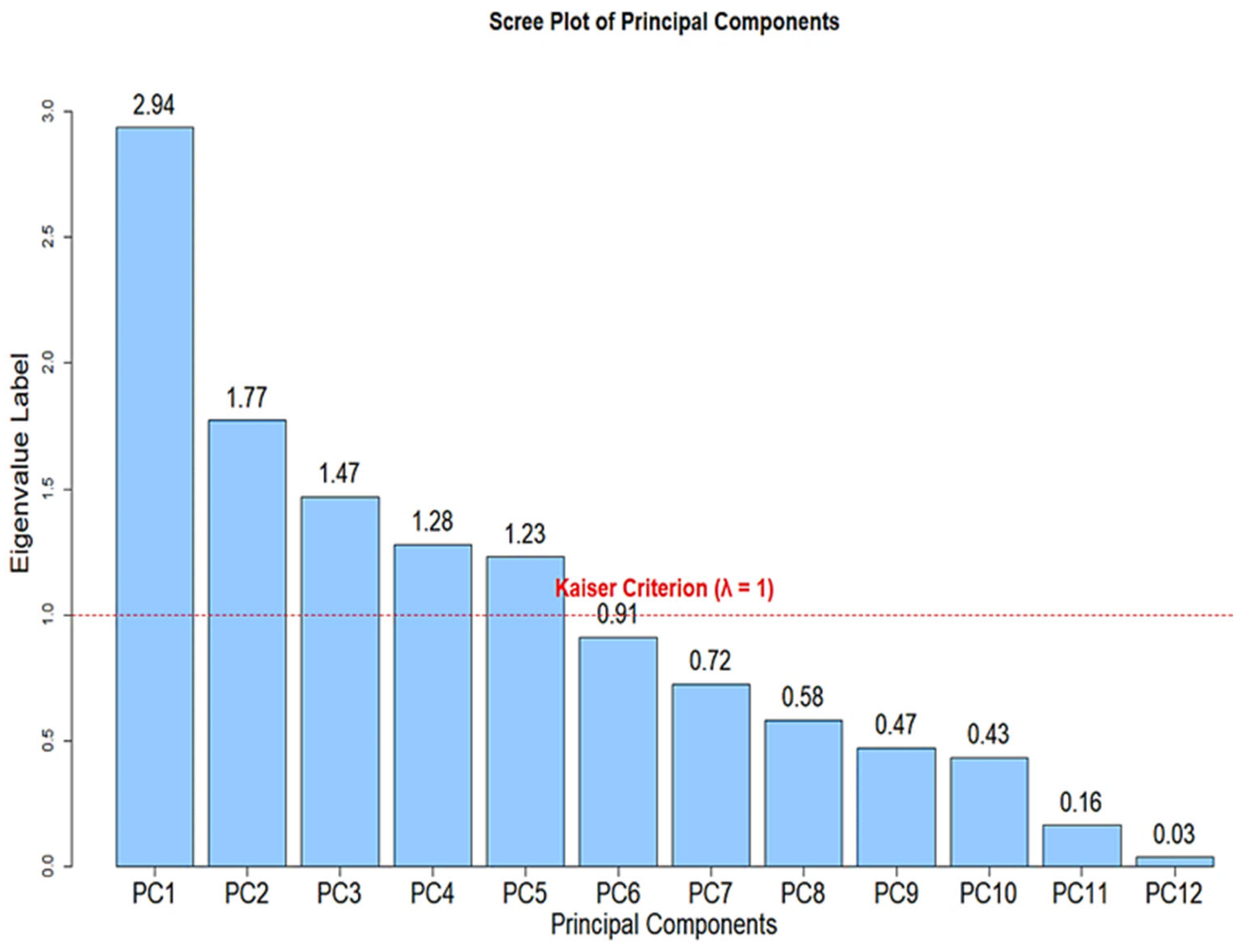
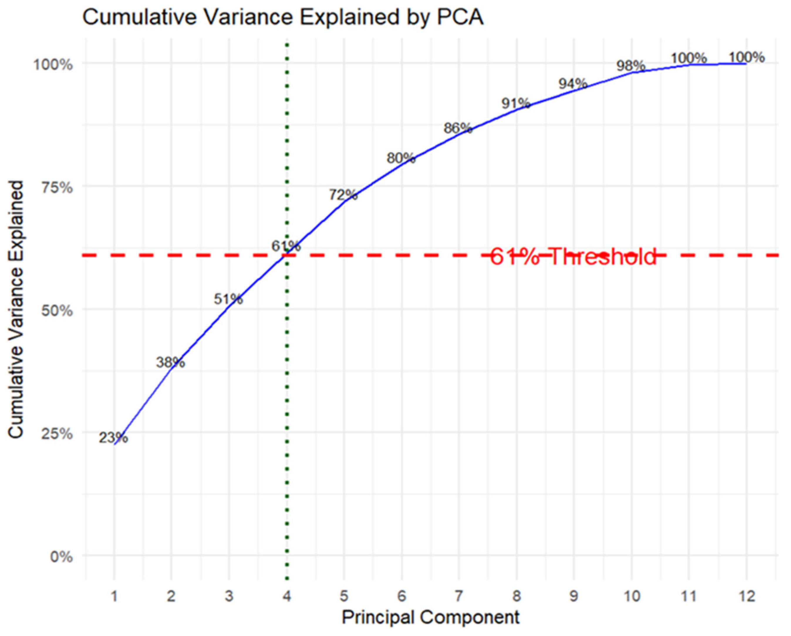
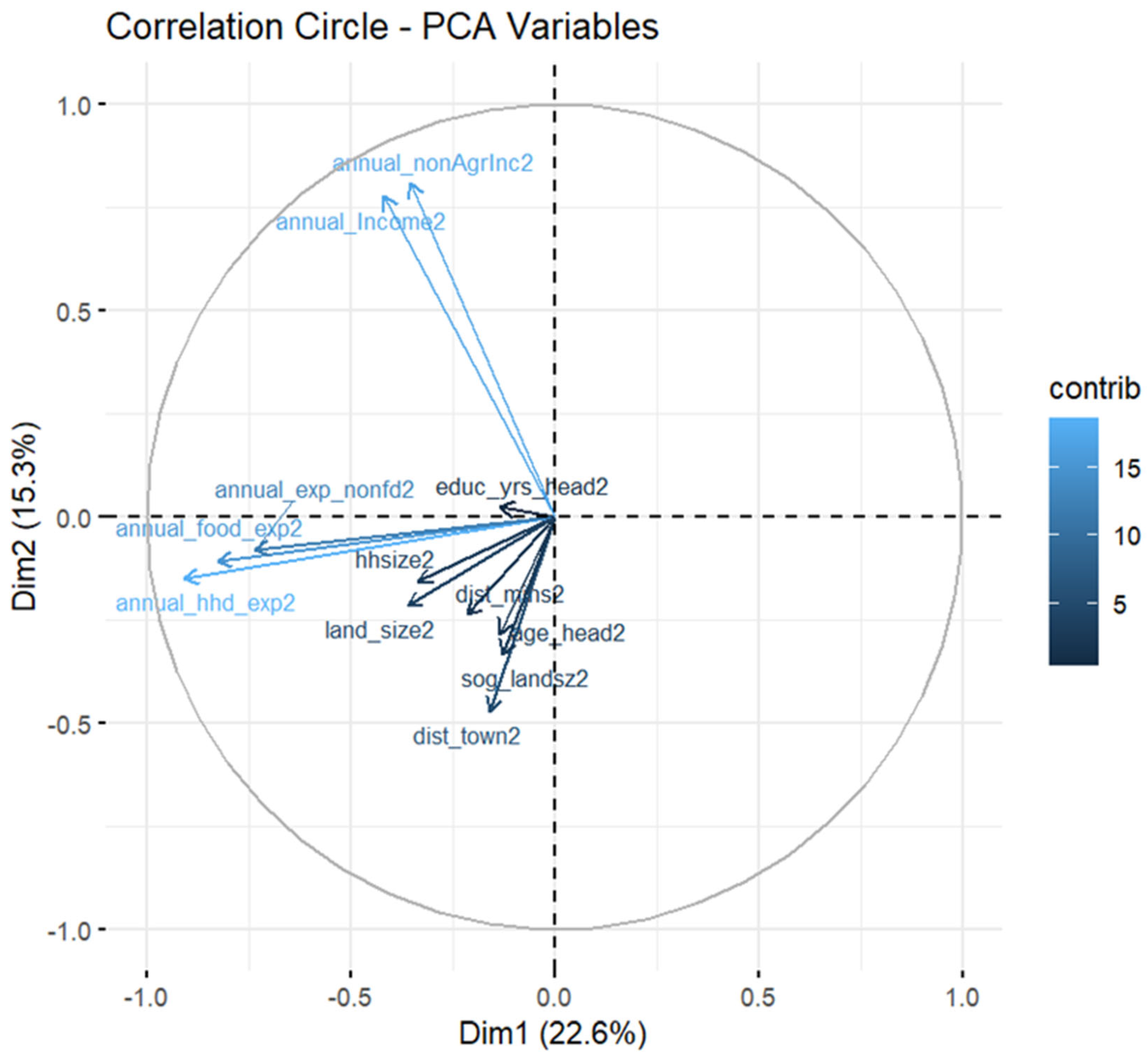
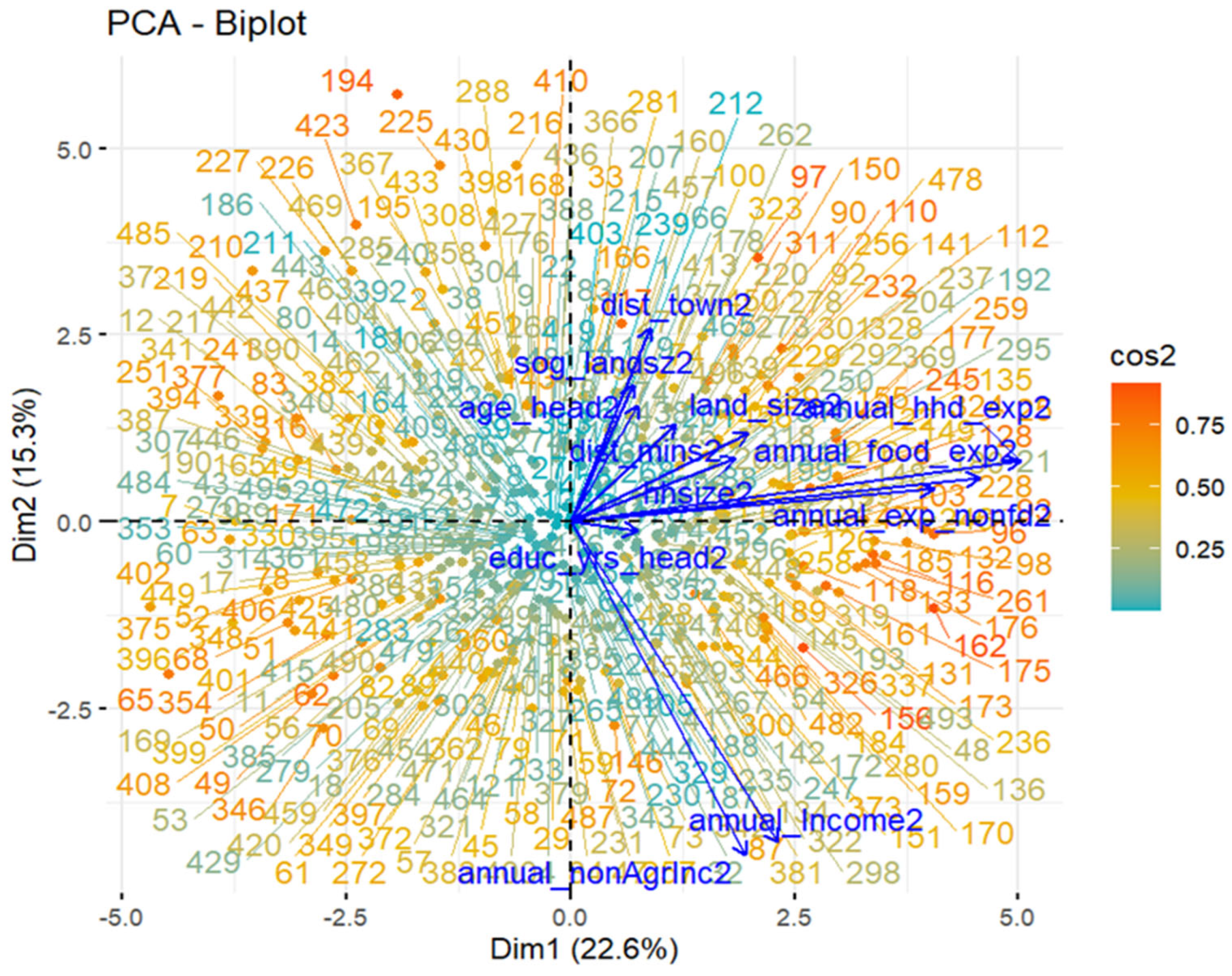
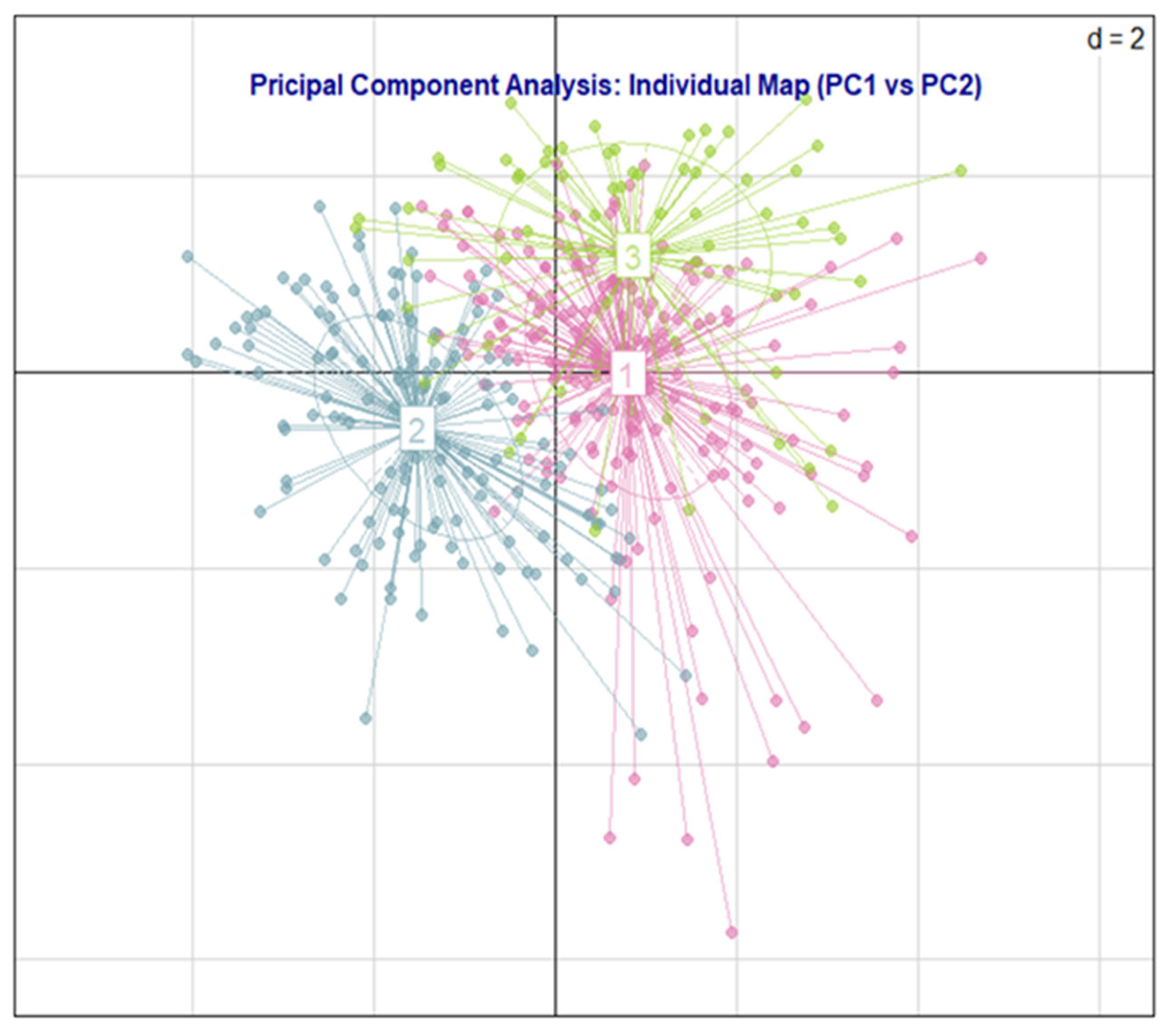
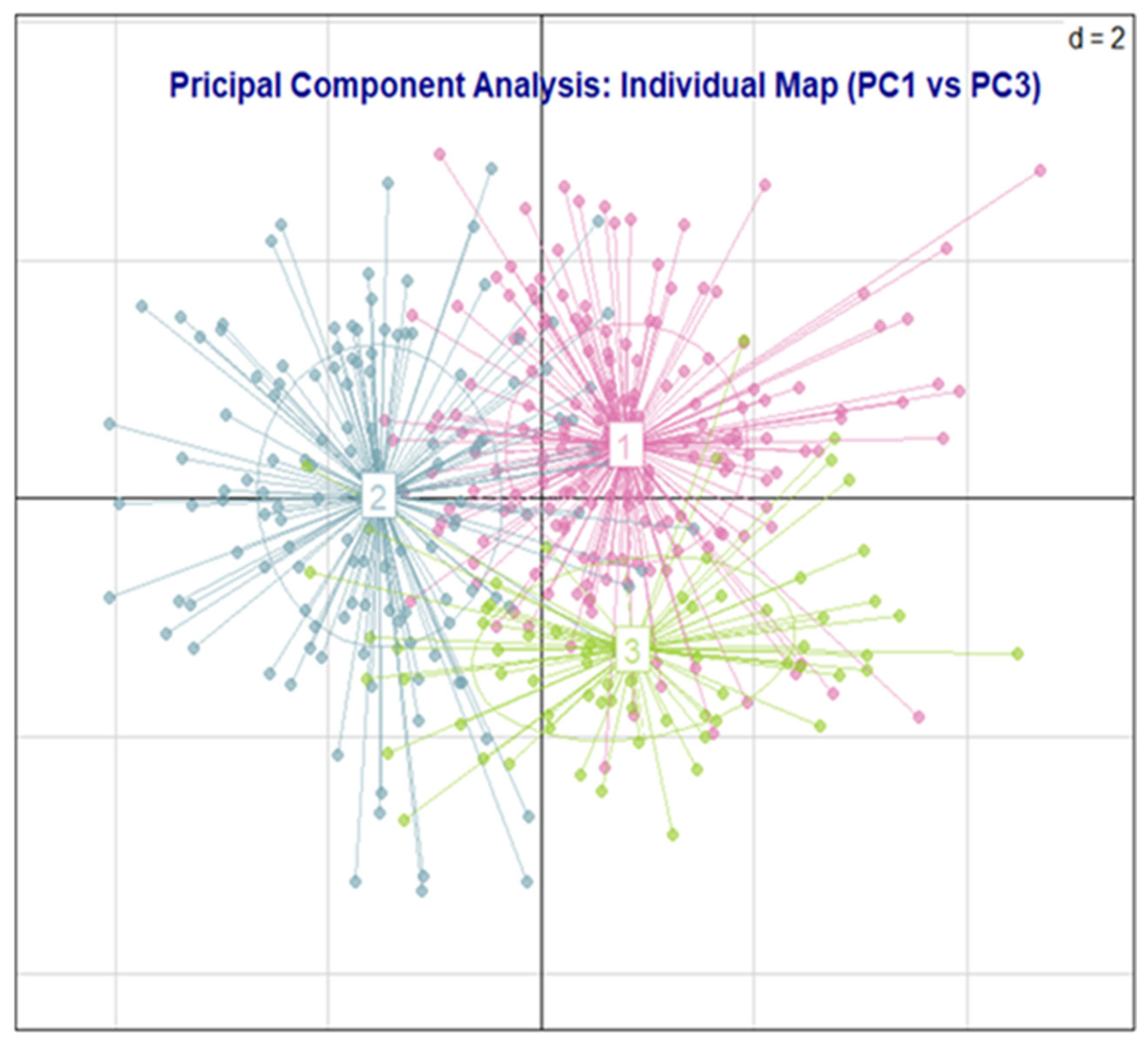
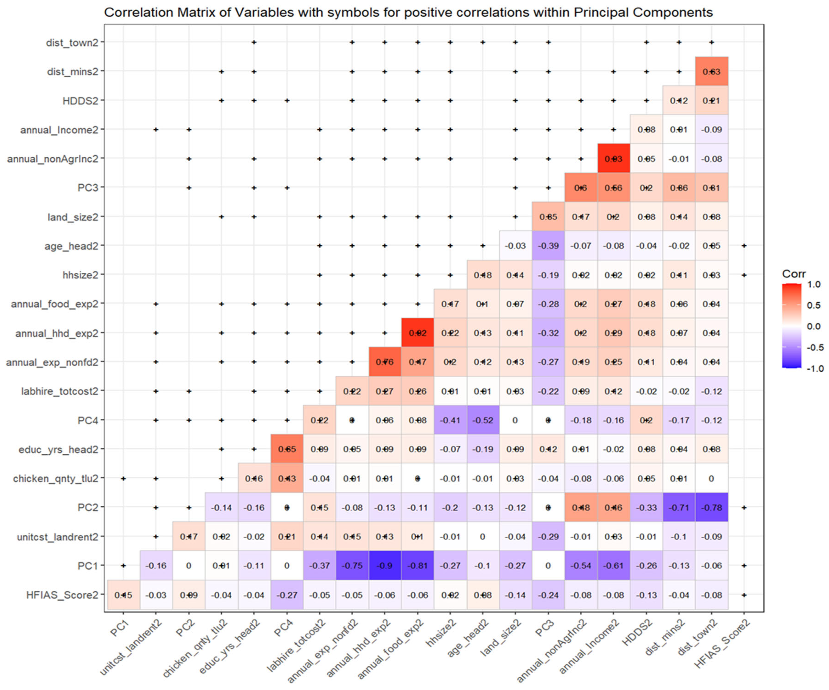
3.2. Principal Component Analysis

Preliminary tests (cf. Table 4 and Appendix A) show that the data is well suited for principal component analysis. The Bartlett's Sphericity Test is significant (χ² = 1911.20; p < 0.001), confirming the existence of significant correlations between the variables. The Kaiser–Meyer–Olkin (KMO) sampling adequacy index reaches 0.78, a value seen as satisfactory for reliable dimension reduction (Figure 6).

In Figure 7, only the first five principal components generated have eigenvalues greater than 1 (Figure 1). Together, these five components explain about 72% of the total variance, the high proportion indicating that these axes capture the crucial information about the variability of characteristics observed in agricultural households and beyond the five components. In this occurrence, it appears that each additional principal component contributes gradually less to the cumulative variance explained, suggesting diminishing returns.

Figure 8 illustrates that the first four principal components (PC1 to PC4) explain approximately 61% of the total variance in the dataset, which indicates that these four components capture most of the meaningful variations present in the data, making them suitable for various multivariate applications such as dimensionality reduction, clustering, typology construction, or input features for further modeling including regression or classification tasks.

The PCA graph (Figure 9) reveals several key observations about the distribution of individuals based on the first two principal components. Most individuals are tightly clustered near the origin, indicating that they have similar values across the principal components. This central concentration suggests low variability among many individuals in the main dimensions and likely reflects a dominant, homogeneous group within the dataset. Despite explaining only 38% of the total variance (22.64% by Dim 1 and 15.30% by Dim 2), these components are still valuable for visualizing the main structure in the data.

The correlation matrix between variables and components (Table 5) highlights the strongest relationships that allow assigning economic meaning to each factorial axis. According to the Kaiser criterion, 5 principal components (PCs) should be retained because their eigenvalues are > 1. This means that, together, these 6 PCs explain a substantial portion of the variance in the data under scrutiny. Principal Component Analysis (PCA) highlights five factorial axes accounting for 72% of the total variance. The first axis (PC1) accumulates 22.64% of the total variance and expresses the dimension of households' living standards and purchasing power. The strongest correlations are observed with variables related to total annual household expenditures (0.909), food expenditures (0.827), and non-food expenditures (0.734). This axis thus opposes low-spending households, characterized by limited consumption, to those with higher expenditures reflecting a better living standard. This dimension therefore represents households’ economic situation and consumption capacity.

The second axis (PC2), which explains 15.30% of the variance, represents the dimension of income and economic diversification. This axis shows the strongest correlations with total annual income (-0.777) and non-agricultural (off farm) income (-0.808). The axis distinguishes households that depend almost exclusively on agriculture from those with diversified incomes, including non-agricultural activities. It highlights an important resilience mechanism related to households' ability to mobilize multiple resources and reduce vulnerability associated with agricultural yield variability. The third axis (PC3), which accounts for 12.77% of the variance, introduces a spatial and structural dimension associated with geographical distance and land size. The most correlated variables are distance to service center (0.587), distance to town (0.501), and land size (0.559). This axis opposes large farms located in areas that are remote from infrastructure and urban markets to small farms neighboring service centers. This illustrates the level of accessibility and territorial integration, suggesting that location directly influences economic opportunities and farmer households’ diversity.

The fourth axis (PC4) captures 10.75% of the variance and represents a dimension of cultural specialization and accessibility (Table 6). The main contributions stem from the proportion of area devoted to sorghum (0.669) and land size (0.514), while the distance to the service center shows a substantially negative correlation (–0.561). This axis describes farms more prone to cash cereal crops, with relatively large areas located in better endowed areas, infrastructure wise. It suggests a more intensive and commercial farming model, illustrative of households with favorable integration into production and supply circuits. Lastly, the fifth axis (PC5), which explains 10.44% of the variance, corresponds to a socio-demographic dimension related to the household head profile.

The dominant variables are the age of the household head (0.668) and years of schooling (-0.710), denoting an opposition between older and less educated operators and younger and better educated operators (Figure 10). This axis illustrates the importance of human capital in the structuring of agricultural systems.

The biplot (Figure 11) highlights the fact that income- and expenditure-related variables are the most influential in shaping Dimension 1, effectively pulling individuals toward the right side of the plot. This indicates that economic capacity and consumption patterns are the primary drivers of variation along this axis. In contrast, variables such as education years, land size, and households’ size contribute more moderately and in different directions, suggesting that education, land endowment, and household composition represent additional, distinct socioeconomic dimensions. Thus, the diversity in vector directions and the spread of individuals across the PCA space reveal a high level of heterogeneity within the dataset, a pattern commonly observed in socioeconomic and agricultural typology studies, where households differ markedly in terms of resources, livelihoods, and living conditions.

In Figure 12 (PC1 vs PC2), the clusters are clearly separated, particularly between Clusters 1 and 2 along the first principal component (Dim 1), which indicates that PC1 captures the main variance distinguishing between these two groups. Cluster 3 overlaps slightly with Cluster 1 but extends upward along the second component (Dim 2), suggesting that PC2 adds further discriminatory power by helping distinguish Cluster 3. This separation pattern supports the conclusion that the three groups represent distinct typologies, shaped by different combinations of socio-economic, demographic, and agricultural variables. In Figure 13 (PC1 vs PC3), the same individuals are projected using PC1 and the third principal component (PC3). The three clusters remain clearly visible, following the same color coding. Here, PC1 continues to effectively separate Cluster 2 from the others, affirming its role as the dominant dimension of variation. However, PC3 provides additional discriminatory power by better separating Cluster 3 downward from Cluster 1 – an aspect that is not fully captured by PC2 in the first graph. This reasserts the multi-dimensional structure of the data, showing that each principal component uniquely contributes to understanding the groupings, and that the cluster separation is robust across different projection planes.

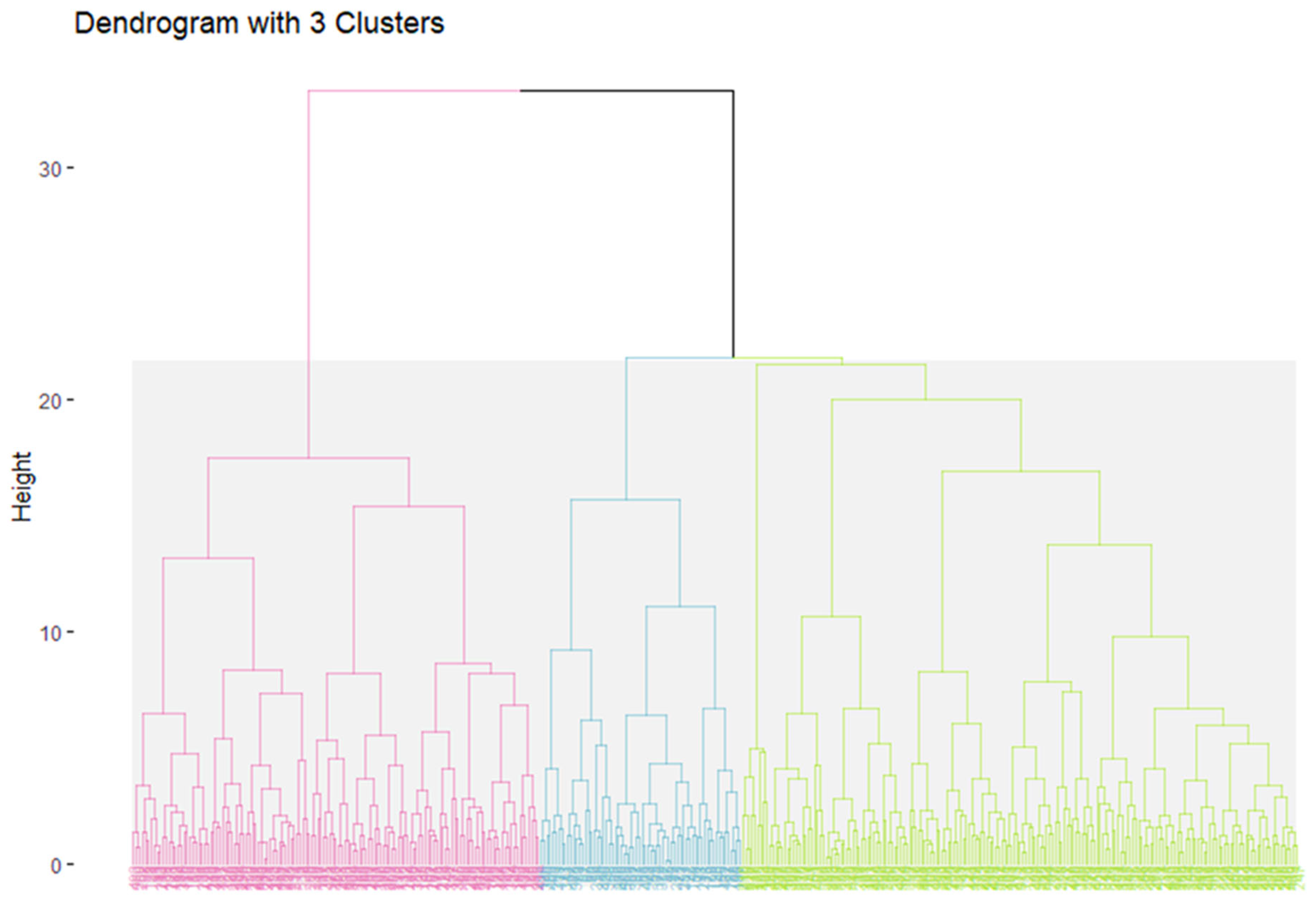
3.3. Cluster Analysis Results

The factorial scores obtained from the five principal components were subjected to a hierarchical classification analysis (Figure 14), followed by consolidation by the method of the mobile centers (k-means). This dual approach, combining an exploratory analysis and statistical optimization, has made it possible to identify three kinds of farmers:

the Basic or Vulnerable Farmers (Type 1); the Well-off Remote Farmers (Type 2) and Educated Farmers in Markets’ Vicinity (Type 3). These 3 types of farmers present marked differences, based on demographic and economic features and tests of equality of means (p < 0.001 for most variables) confirming the significance of these distinctions, guaranteeing the internal consistency of the typology and its analytical relevance (Table 7).

Type 1, classified as Basic or Vulnerable Farmers, groups the most vulnerable fraction of agricultural operators. These farmers are characterized by modest incomes (averaging 370,600 SDG/year) and limited annual expenditures, indicating a low standard of living. Household heads have a restricted level of education (averaging 6.7 years of schooling), which limits their ability to access information, innovation, and formal markets. With an average farm size of approximately 15 hectares, these households practice subsistence agriculture, often relying on rainfall and being poorly diversified. The minimal use of hired labor (averaging 15,533 SDG/year) confirms their low productive intensity and dependence on family labor. Considered together, all these characteristics reflect a situation of structural vulnerability, whereby economic and human constraints combine to limit growth prospects and resilience against climate or economic shocks. Type 2, designated as Well-off Remote Farmers, groups relatively wealthy households characterized by larger land allocations (averaging 21 ha) and higher average incomes (averaging 492,000 SDG/year). These households also show the highest levels of both food and non-food expenditures and are distinguished by intensive use of hired labor (averaging 61,700 SDG/year).

This profile suggests a commercial trend/proneness and increased capacity for investment in agricultural production. However, their farms are in geographically isolated areas, with an average distance of approximately 63 minutes from the nearest service. This spatial isolation indicates that these farmers compensate for logistical costs and difficulties in accessing markets by utilizing large land areas and mobilizing significant productive resources. Thus, Type 2 embodies the model of capitalized – although peripheral – agriculture, whose performance depends heavily on land availability and the ability to bear the high transaction costs associated with distance. Type 3, classified as Educated Farmers in Markets’ Vicinity, represents a more limited category in terms of numbers, despite being highly significant from a structural standpoint. This group includes the youngest farmers and most educated (average 8.3 years of schooling), indicating higher human capital. They operate small farming areas (average 7 ha) but benefit from proximity to urban centers and services (average 13 minutes). Despite their limited landholdings, these households pay the highest rents, reflecting strong land pressure in peri-urban areas. These farms thus combine high human capital, good accessibility, and land optimization strategies, reflecting a transition toward connected and innovative entrepreneurial agriculture.

The correlation matrix illustrates the relationships among key socioeconomic variables and the four principal components (PC1–PC4). Annual income, off-farm income, household expenditure, and food expenditure are all highly interrelated correlation coefficients above 0.9 (Figure 15). This suggests that higher total income is closely tied to higher spending, particularly on food, confirming the internal consistency of the dataset and the central role of income in household welfare. Similarly, land size and household size show a mild positive relationship with income and expenditure, indicating that larger households and farms tend to have slightly higher earnings and consumption levels. In contrast, PC1 is negatively correlated with most expenditure and income variables (–0.7 to –0.9), suggesting that PC1 likely captures a gradient of household economic capacity – where higher PC1 values correspond to poorer, lower-income households.

PC2, on the other hand, shows moderate positive correlations with income and expenditure (0.4 to 0.6), implying that it may represent another dimension of wealth or production intensity. PC3 and PC4 have weaker and more scattered correlations, indicating that they capture more specific or secondary aspects of variability, such as education, distance to services, or labor costs. Interestingly, the food insecurity score exhibits weak or slightly negative correlations with income and expenditure, reinforcing the notion that households with higher income tend to experience lower food insecurity. The education level of the household head shows moderate positive correlations with expenditure and income, indicating that education contributes to better economic outcomes. Distance-related variables display weak and sometimes negative correlations with economic variables, suggesting that households farther from towns or markets may have less access to income-generating opportunities.

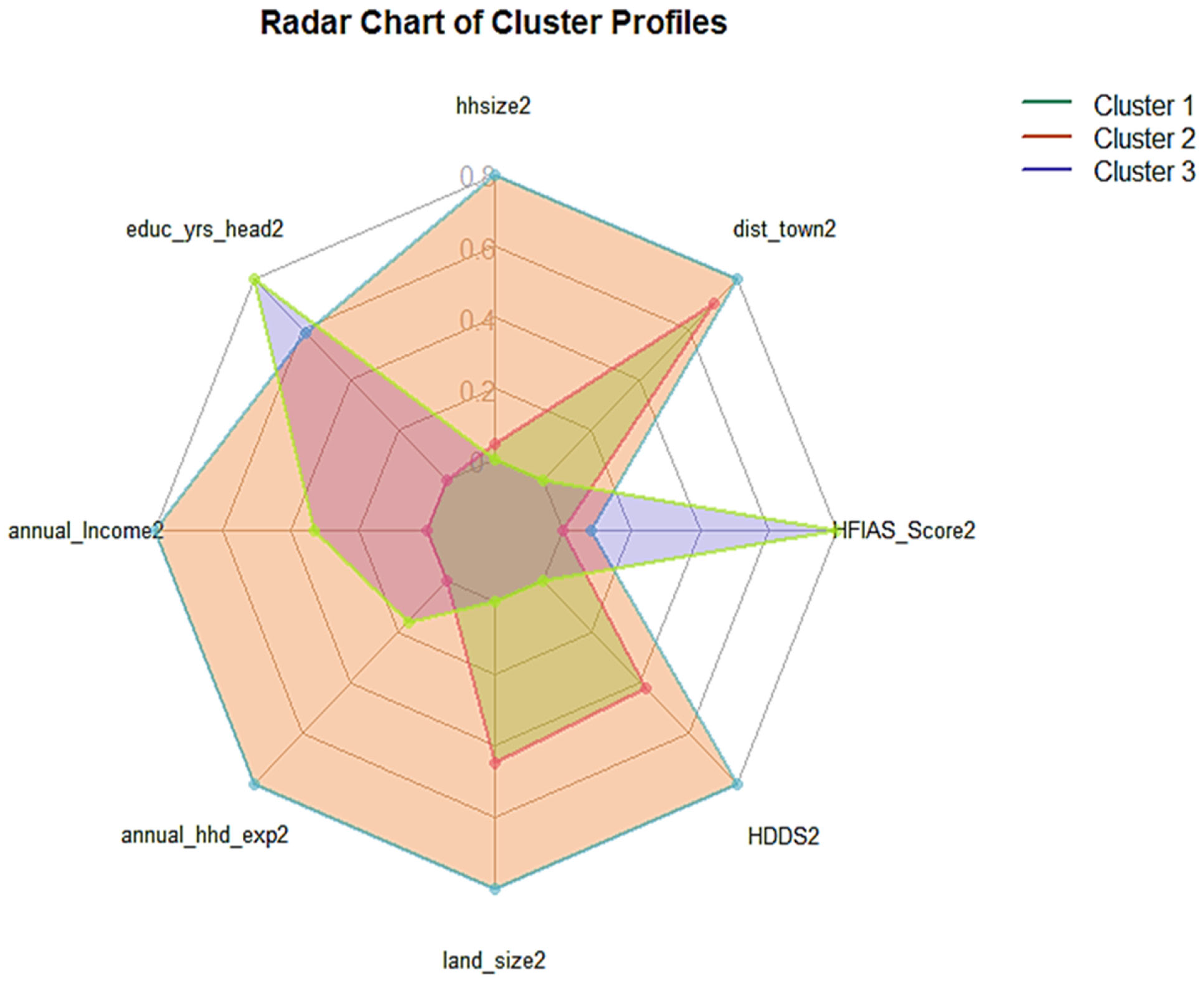
3.4. Radar Chart of Cluster Profiles

The radar chart (Figure 16) visually confirms the robustness and consistency of the typological profiles identified among Sudanese farmers. Type 2 clearly dominates economic axes, mostly regarding income, expenses, and use of hired labor, reflecting financial and productive superiority. Type 3, in turn, is distinguished by high scores on education, geographical proximity, and income diversification variables, confirming its more urban and innovative nature. Conversely, Type 1 shows low values across all dimensions, illustrating its economic and social marginalization. Each of these categories calls for differentiated policy responses: development of infrastructure and reduction of logistics costs for remote farmers, productive strengthening programs and social support for vulnerable households, as well as support for agricultural entrepreneurship and market access for educated young producers.

With respect to the Household Dietary Diversity Score (HDDS), clusters 2 and 3 display comparable distributions, with dietary diversity scores ranging between 6 and 13 (Figure 17). In both clusters, 50% of the households fall within the 9 to 11 range, indicating a relatively similar and moderate level of dietary diversity, as Cluster 1 shows a similar overall range. However, its interquartile range is slightly shifted, with half of the population exhibiting dietary diversity scores between 8 and 11, suggesting marginally lower center-marked tendency compared to clusters 2 and 3. In contrast, the Household Insecurity Access Scale (HFIAS) reveals clearer differences across clusters. Clusters 1 and 2 exhibit a wide dispersion at the upper end of the scale, indicating substantial variability in food insecurity levels and the presence of highly food-insecure households. Cluster 3, on the other hand, shows much lower dispersion, with only three outliers, reflecting more homogeneous conditions. Importantly, cluster 2 records the highest levels of food insecurity, followed by cluster 1, whereas cluster 3 demonstrates the lowest food insecurity levels overall. These results suggest that cluster 3 represents the most food-secure group, while clusters 1 and especially cluster 2 happen to be more vulnerable in terms of household food access.

3.5. Multinomial Logistic Regression Results

The multinomial logistic regression model (Table 7) identifies the factors influencing the likelihood of belonging to a specific farmer’s type group. The marginal effects analysis (Table 8) reveals clear patterns in how household characteristics, socio-economic variables, and geographic location influence the probability of a household belonging to each type of group. Household size significantly increases the likelihood of being in Type 2 (p < 0.01) and decreases the probability of being in Type 3 (p < 0.01), suggesting that larger households are more likely to belong to type 2 and less likely to be in Type 3. Similarly, the age of the household head shows a small but statistically significant positive association with Type 2 (p < 0.05) and a negative effect on Type 3 (p < 0.05), indicating that older household heads are more likely to be in Type 2 and less likely in Type 3. Education of the household head is associated with a lower probability of Typology 1 (baseline) and a higher probability of Type 2 (p < 0.05), reinforcing the idea that more educated heads are more likely to be in more economically engaged or resilient types of farmers.

Remoteness, measured by distance (in minutes) to services, significantly increases the probability of being in Types 1 and 2 (both p < 0.01) while reducing the likelihood of Type 3 (p < 0.01), suggesting that Type 3 households are more likely to be in accessible areas. Land ownership, particularly sorghum land size, follows a similar pattern – with positive associations for Types 1 and 2 (p < 0.01) and a strong negative association with Type 3 (p < 0.01) – highlighting the importance of productive agricultural assets in typology membership. Non-food expenditures are negatively associated with Type 1 (p < 0.05) and positively (though less strongly) associated with Type 3 (p < 0.1), while hired labor costs also show a marginally significant positive effect on Type 3 (p < 0.1). This may reflect differences in livelihood strategies or investment capacities across typologies.

Regional effects are also pronounced. Households in North Kordofan show significantly higher probabilities of belonging to Types 1 (p < 0.05) and 2 (p < 0.1), and a much lower probability of being in Type 3 (p < 0.01). Likewise, South Darfur is associated with higher probabilities of Type 1 (p < 0.01) and Type 2 (p < 0.1) and a significantly lower likelihood of Type 3 (p < 0.01). West Kordofan and White Nile also display similar directional effects, all statistically significant. Additionally, West Darfur shows a significant negative association with Type 3 (p < 0.1), while regions such as Kassala and Gedarif also demonstrate significant effects (p < 0.05, respectively) on Type 3 reflated membership. These geographic patterns indicate that household typology is shaped not only by demographic and economic factors but also by broader contextual and regional dynamics. Overall, the results underscore that typology classification is influenced by a combination of household structure, economic status, remoteness, and location (geographical feature). The statistically significant effects across multiple variables point to meaningful distinctions in household strategies, market access, and vulnerability profiles among the different typology groups.

4. Discussion

As outcome of this study, the results reveal that the differentiation of Sudanese agricultural households revolves around three major types of farmers: living standards, income diversification, geographical location, productive specialization, and socio-demographic profile. This structure confirms the multidimensional nature of agricultural systems, already highlighted by [15,26] in different African contexts elsewhere. To sum it up, variables related to age and education confirm a generational and educational gap already observed by [17], whereby young, educated farmers are more prone to move towards modern and commercial agriculture. From these components, hierarchical classification and the moving centers method have made it possible to identify three distinct types of agricultural households, reflecting contrasting productive and social logics.

The first group, vulnerable farmers, brings together the most economically fragile households. Their low annual income, limited level of education, and restricted access to productive resources reflect a dependence on rain-fed agriculture and a subsistence economy. These results corroborate those of [43] in South Africa and [44] in Tanzania, which show that rural poverty is typified by low technological adoption and increased vulnerability to environmental shocks. The existence of this category highlights the limitations of one-size-fits-all agricultural policies, often unable to reach marginalized small-scale producers. The second group, well-off remote farmers, presents a paradoxical situation: these households have large land areas and high agricultural incomes, but their distance from infrastructure and markets hinders their economic integration. This configuration illustrates the "abundance isolation" paradox described by [16] in Niger and confirmed by [45] in Ethiopia. Farmers of this type have strong production and investment potential, but their yields remain limited by poor transport networks and agricultural services. These households represent the productive core of Sudanese agriculture, but their contribution to rural development will largely depend on targeted land use policies and better access to value chains. As emphasized by [15] and [11], recognizing and valuing the diversity of farming systems is an essential condition for the sustainable structural transformation of the sector. An extensive spread of this parameter is present in both indicators, especially for HFIAS, underscoring the inner-State heterogeneity in household experiences. This intra-regional variation, especially evident in Central Darfur and White Nile, suggests that food insecurity is not evenly distributed and that targeted, localized interventions are necessary.

Lastly, the third group, Educated Farmers in Markets’ Vicinity, embodies a dynamic of agricultural modernization. These households, led by younger and most educated heads, cultivate small areas located near cities. Despite their reduced size, they stand out through strong diversification of their income and a trend to move towards intensification. These results confirm the observations of [17] and [38], stating that land pressure and urban proximity favor more intensive practices and rapid adoption of innovations. Moreover, the association between education and performance observed in this group is in accordance with the conclusions of [11] and [46], who emphasize that training and pluri-activity stimulate the transition towards entrepreneurial agriculture, which is more ‘connected’ and sustainable. This category thus illustrates the occurrence of a generation of emerging farmers, capable of penetrating and fitting into the urban economy and playing a driving role in the structural transformation of the sector. These three types reflect the contrasting trajectories of Sudanese agriculture: a vulnerable but socially dominant survival-based agriculture, an extensive capital-endowed agriculture but isolated, and a proximity agriculture that is underpinned by education and innovation. This segmentation abides by a logic comparable to that observed by [28] and [15] in West Africa, whereby differentiation is based on the articulation between land capital, human capital, and spatial connectivity. It also highlights the need for a differentiated approach to agricultural policies, based on the recognition of this internal diversity, as recommended by [9] and [14].

5. Methodological and Empirical Approach Contribution and Implications for Theory

The study illustrated that the multinomial approach; principal component analysis (PCA) and cluster analysis (CA) utilized are suitable tools for identifying important socioeconomic characteristics of typical farmers types involving in Sorghum production in Sudan and corroborate with other scholars studies [47]. Thus, the choice of PCA and CA, was justified in this study due to the complexity and multidimensional nature Sudan farmer diversity factors. Analysis allowed for the simultaneous examination of numerous variables to capture the inherent diversity among farmers, reducing data dimensionality while retaining critical variance. This approach enabled the classification of farmers into distinct types based on socioeconomic characteristics, and multinomial regression providing a comprehensive understanding of the factors like gender, age, food security, education level, TLU, food security, land size etc. which influencing the likelihood of belonging to a specific farmer’s type groups. The results of this study full fill the gap highlighted in previous studies in Sudan [18,21,48,49,50] and around the world [2,7,20,51,52,53] and are in line with those of SDG 1 and SDG 2, and other scholars [7,25,54]. In particular, the objectives of increasing agricultural production and fighting poverty and hunger [55]. This study identified three distinct farm types that can be targeted for scaling up and readiness for agricultural policy, food security and rural development and methodology can be adapted to different situations and objectives of farm typology studies in fragile context.

6. Study Limitations

This study has certain limitations. Firstly, the data used does not capture all the qualitative dimensions related to institutional dynamics or cultural practices, which also influence agricultural differentiation [13]. Secondly, the typology developed is based on a static analysis; however, agricultural typologies are dynamic and evolve under the effect of economic, climatic, and social transformations. Last but not the least, the classification relies on quantitative variables without integrating behavioral indicators, which are yet essential for a more comprehensive understanding of agricultural systems [11]. Despite these limitations, the results offer important practical implications, providing an empirical basis for designing differentiated policies. Also highlighted are: Targeted support for vulnerable households through capacity building, investment in rural infrastructure to connect isolated farms; and promotion of agricultural entrepreneurship and technical training for educated young farmers. Hence, the analysis reveals and asserts clear regional disparities in food security across Sudan. Furthermore, the different Principal Component visualizations perform through this study is particularly powerful for identifying different farmer types within a unique characteristic, guiding further analysis or policy targeting in agricultural and development research particularly in fragile context like Sudan where this kind of study is rare. Overall, this typology makes an empirical foundation for more effective planning and implementation of agricultural development programs in Sudan, supporting the design of inclusive, evidence-based rural policies aimed at enhancing productivity, equity, and sustainability.

7. Conclusions and Recommendations

The study consistently developed a typology of Sudanese farmer households using a multivariate approach, combining Principal Component Analysis (PCA) and clustering techniques. Each cluster was therefore shaped by varying socio-economic, demographic, and agricultural characteristics, hence bringing the study to reveal three distinct farmer groups based on household characteristics, farm resources, and socio-economic indicators. These typologies provide a clear structure for understanding the diversity among rural households and highlight key differentiating factors such as landholding size, income sources, education, and food security status. The findings underline the importance of tailored policy interventions. Each farmer typefaces unique constraints and opportunities, suggesting that “one-size-fits-all” agricultural policies are ineffective. Instead, targeted strategies that account for household diversity – such as improving market access for better-off farmers or enhancing food security and resilience for more vulnerable households – are needed.

Results also demonstrate a clear spatial pattern: States in the eastern regions have higher educational attainment but smaller families, while western and southern States exhibit larger household sizes and, overall, lower levels of education. These disparities may reflect differences in economic opportunities, infrastructure, cultural norms, and access to education services across Sudan’s regions. Land access and sorghum cultivation are unevenly distributed across Sudan’s States. The southern and eastern regions appear to have larger agricultural holdings and greater emphasis on sorghum production, while western and northeastern States show smaller, more constrained land resources. These disparities may reflect variations in agroecological potential, population density, land tenure systems, and local livelihood strategies. The overall trend reflects a relatively low level of dietary diversification, which may not be sufficient to ensure balanced nutrition. This pattern highlights potential vulnerabilities in food systems, particularly in terms of access to a diverse and nutritionally adequate diet. which may be associated with reduced agricultural productivity, poor market access, or economic hardship.

The multinomial regression analysis revealed that variables such as education level, household size, landholding size, income composition (both agricultural and non-agricultural), food security indicators (HFIAS and HDDS), and livelihood strategies significantly influence the probability of belonging to a particular typology. Type 1 emerged as the most vulnerable group, characterized by small land sizes, low educational attainment, limited non-agricultural income, and high levels of food insecurity. Type 2 represents moderately secure households with a balance between agricultural and non-agricultural income sources but still facing food insecurity risks. In contrast, Type 3 includes better-off households, benefiting from larger landholdings, diversified income streams, higher education, and boosted food security.

These results underscore the need for differentiated agricultural and rural development strategies. For type 1, targeted support such as input subsidies, extension services, and access to credit is essential to enhance productivity and resilience. Type 2 would benefit from policies that promote livelihood diversification through vocational training and support for small-scale non-farm enterprises. As for Type 3, interventions should focus on expanding market access, integrating households into value chains, and fostering agribusiness development. Additionally, land reform policies are necessary to address inequality in land access, particularly affecting the most vulnerable households. Education and literacy programs must be promoted and strengthened across all clusters to empower households to make informed decisions and improve their economic standing. Food security and nutrition-focused programs should be prioritized in regions dominated by Types 1 and 2. Given the geographic variability in Cluster distribution, development interventions must be spatially tailored to reflect the specific needs and capacities of different regions. Ultimately, the combined analytical approach provides an empirical foundation for designing inclusive and efficient policies that support sustainable rural development and improve livelihoods in Sudan.

References

1. Ehab, E.A.M.F. ARIMA, Forecasting, Sorghum and Sudan; 2016. [Google Scholar]
2. Nkosi, Z.; Marwa, N.; Akinrinde, O.O. Exploring the Feasibility of Sorghum Farming in South Africa Using Garrett’s Ranking Technique. Agriculture 2024, 14, 2348. [Google Scholar] [CrossRef]
3. Hosseini, E.; Tsegay, Z.T.; Smaoui, S.; Elfalleh, W.; Antoniadou, M.; Varzakas, T.; Caraher, M. One Health Approaches to Ethical, Secure, and Sustainable Food Systems and Ecosystems: Plant-Based Diets and Livestock in the African Context. Foods 2025, 15, 85. [Google Scholar] [CrossRef]
4. USDA Sorghum | USDA Foreign Agricultural Service. Available online: https://www.fas.usda.gov/data/production/commodity/0459200 (accessed on 16 December 2025).
5. Grenier, C.; Bramel, P.J.; Dahlberg, J.A.; El-Ahmadi, A.; Mahmoud, M.; Peterson, G.C.; Rosenow, D.T.; Ejeta, G. Sorghums of the Sudan: Analysis of Regional Diversity and Distribution. Genet. Resour. Crop Evol. 2004, 51, 489–500. [Google Scholar] [CrossRef]
6. Wang, M.; Ahmad, I.; Hussien Ibrahim, M.; Qin, B.; Zhu, H.; Zhu, G.; Zhou, G. Differential Responses of Two Sorghum Genotypes to Drought Stress at Seedling Stage Revealed by Integrated Physiological and Transcriptional Analysis. Agriculture 2025, 15, 1780. [Google Scholar] [CrossRef]
7. Dahlberg, J.A.; Burke, J.J.; Rosenow, D.T. Development of a Sorghum Core Collection: Refinement and Evaluation of a Subset from Sudan. Econ. Bot. 2004, 58, 556–567. [Google Scholar] [CrossRef]
8. Smits, E.; Kuijpers, R.; Miteng, J.A.; Deng Chol, D.; Mono, T.T.; Francesconi, N. Is Seed Aid Distribution Still Justified in South Sudan? World Dev. Perspect. 2024, 36, 100638. [Google Scholar] [CrossRef]
9. Alvarez, S.; Timler, C.J.; Michalscheck, M.; Paas, W.; Descheemaeker, K.; Tittonell, P.; Andersson, J.A.; Groot, J.C.J. Capturing Farm Diversity with Hypothesis-Based Typologies: An Innovative Methodological Framework for Farming System Typology Development. PLoS ONE 2018, 13, 1–24. [Google Scholar] [CrossRef]
10. Tittonell, P.; Bruzzone, O.; Solano-Hernández, A.; López-Ridaura, S.; Easdale, M.H. Functional Farm Household Typologies through Archetypal Responses to Disturbances. Agric. Syst. 2020, 178. [Google Scholar] [CrossRef]
11. Huber, R.; Bartkowski, B.; Brown, C.; El Benni, N.; Feil, J.-H.; Grohmann, P.; Joormann, I.; Leonhardt, H.; Mitter, H.; Müller, B. Farm Typologies for Understanding Farm Systems and Improving Agricultural Policy. Agric. Syst. 2024, 213, 103800. [Google Scholar] [CrossRef]
12. Benitez-Altuna, F.; Trienekens, J.; Gaitán-Cremaschi, D. Categorizing the Sustainability of Vegetable Production in Chile: A Farming Typology Approach. Int. J. Agric. Sustain. 2023, 21, 2202538. [Google Scholar] [CrossRef]
13. Beza, E.; Steinke, J.; Van Etten, J.; Reidsma, P.; Fadda, C.; Mittra, S.; Mathur, P.; Kooistra, L. What Are the Prospects for Citizen Science in Agriculture? Evidence from Three Continents on Motivation and Mobile Telephone Use of Resource-Poor Farmers. PLOS ONE 2017, 12, e0175700. [Google Scholar] [CrossRef]
14. Jansma, J.E.; Veen, E.J.; Müller, D. Beyond Urban Farm and Community Garden, a New Typology of Urban and Peri-urban Agriculture in Europe. Urban Agric. Reg. Food Syst. 2024, 9, e20056. [Google Scholar] [CrossRef]
15. Kuivanen, K.S.; Alvarez, S.; Michalscheck, M.; Adjei-Nsiah, S.; Descheemaeker, K.; Mellon-Bedi, S.; Groot, J.C.J. Characterising the Diversity of Smallholder Farming Systems and Their Constraints and Opportunities for Innovation: A Case Study from the Northern Region, Ghana. NJAS Wagening. J. Life Sci. 2016, 78, 153–166. [Google Scholar] [CrossRef]
16. Priegnitz, U.; Lommen, W.J.M.; Onakuse, S.; Struik, P.C. A Farm Typology for Adoption of Innovations in Potato Production in Southwestern Uganda. Front. Sustain. Food Syst. 2019, 3, 1–15. [Google Scholar] [CrossRef]
17. Bagagnan, A.R.; Berre, D.; Webber, H.; Lairez, J.; Sawadogo, H.; Descheemaeker, K. From Typology to Criteria Considered by Farmers: What Explains Agroecological Practice Implementation in North-Sudanian Burkina Faso? Front. Sustain. Food Syst. 2024, 8, 1386143. [Google Scholar] [CrossRef]
18. Salim, E.R.A. Fortified Sorghum as a Potential for Food Security in Rural Areas by Adaptation of Technology and Innovation in Sudan. 2017, 1. [Google Scholar]
19. BabekirElgali, M.; Mustafa, R.H.; Kirschke, D.; Khair, A.Y.M.; Maruod, M.E. SORGHUM PERFORMANCE UNDER CLIMATE CHANGE IN SUDAN. 2016. [Google Scholar]
20. Mwadalu, R.; Mwangi, M. The Potential Role of Sorghum in Enhancing Food Security in Semi-Arid Eastern Kenya: A Review. J. Appl. Biosci. 2013, 71, 5786. [Google Scholar] [CrossRef]
21. Ahmed, N.; Elrasheed, M. Socioeconomic Factors Affecting Sorghum Productivity in the Rain-Fed Sector of Gadarif State, Sudan. Asian J. Agric. Ext. Econ. Sociol. 2016, 10, 1–6. [Google Scholar] [CrossRef]
22. Alvarez, S.; Paas, W.; Descheemaeker, K.; Tittonell, P.; Groot, J. Constructing Typologies, a Way to Deal with Farm Diversity: General Guidelines for the Humidtropics. Report for the CGIAR Research Program on Integrated Systems for the Humid Tropics. Plant Sci. Group 2014, Report for, 1–37. [Google Scholar]
23. Adzawla, W.; Atakora, W.K.; Kissiedu, I.N.; Martey, E.; Etwire, P.M.; Gouzaye, A.; Bindraban, P.S. Characterization of Farmers and the Effect of Fertilization on Maize Yields in the Guinea Savannah, Sudan Savannah, and Transitional Agroecological Zones of Ghana. EFB Bioeconomy J. 2021, 1, 100019. [Google Scholar] [CrossRef]
24. Bidogeza, J.C.; Berentsen, P.B.M.; Graaff, J.; Oude Lansink, a. G.J.M. Multivariate Typology of Farm Households Based on Socio-Economic Characteristics Explaining Adoption of New Technology in Rwanda. AAAE Ghana Conf. 2007, 275–281. [Google Scholar]
25. Nabahungu, N.L.; Mirali, J.C.; Simbeko, G.; Amato, S.; Mirali, G.M.; Muhindo, P.M.; Kitangala, C.; Balangaliza, F.B.; Nguezet, P.-M.D.; Kintche, K.; et al. Farmer Typology and Adoption of Improved Cassava Production Technologies in the Eastern Democratic Republic of the Congo. CABI Agric. Biosci. 2025, 0018. [Google Scholar] [CrossRef]
26. Tittonell, P.; Muriuki, A.; Shepherd, K.D.; Mugendi, D.; Kaizzi, K.C.; Okeyo, J.; Verchot, L.; Coe, R.; Vanlauwe, B. The Diversity of Rural Livelihoods and Their Influence on Soil Fertility in Agricultural Systems of East Africa – A Typology of Smallholder Farms. Agric. Syst. 2010, 103, 83–97. [Google Scholar] [CrossRef]
27. Alvarez, S.; Paas, W.; Descheemaeker, K.; Tittonell, P.; Groot, J.C.J. Constructing Typologies, a Way to Deal with Farm Diversity: General Guidelines for the Humidtropics. Rep. CGIAR Res. Program Integr. Syst. Humid Trop. Plant Sci. Group Wagening. Univ. Neth. 2014, 1–37. [Google Scholar]
28. Tittonell, P.A. Farming Systems Ecology: Towards Ecological Intensification of World Agriculture; Wageningen Universiteit: Wageningen, 2013; ISBN 978-94-6173-617-8. [Google Scholar]
29. Shifat, S. Sorghum Farming in Sudan: A Deep Dive into Its Impact on the Economy - The African Dreams ! 2025. [Google Scholar]
30. M Elamin, E. Economic Consideration and Model Development Spatial Trade for Sorghum and Millet Staple Food in Sudan. Agric. Res. Technol. Open Access J. 2018, 14. [Google Scholar] [CrossRef]
31. WFP Celebrates Sorghum Harvest in Eastern Sudan under World Bank Managed THABAT Project | World Food Programme. Available online: https://www.wfp.org/news/wfp-celebrates-sorghum-harvest-eastern-sudan-under-world-bank-managed-thabat-project (accessed on 16 December 2025).
32. Abarca, R.M. Practical Guide to Principal Component Mathods in R:PCA, (M)CA, FAMD, MFA, HCPC, Factorextra. Nuevos Sist. Comun. E Inf. 2021, 2013–2015. [Google Scholar]
33. Simbeko, G.; Nguezet, P.-M.D.; Sekabira, H.; Yami, M.; Masirika, S.A.; Bheenick, K.; Bugandwa, D.; Nyamuhirwa, D.-M.A.; Mignouna, J.; Bamba, Z.; et al. Entrepreneurial Potential and Agribusiness Desirability among Youths in South Kivu, Democratic Republic of the Congo. Sustainability 2023, 15, 873. [Google Scholar] [CrossRef]
34. Vyas, S.; Kumaranayake, L. Constructing Socio-Economic Status Indices: How to Use Principal Components Analysis. Health Policy Plan. 2006, 21, 459–468. [Google Scholar] [CrossRef]
35. Mustapha, S. Application of Multinomial Logistic to Smallholder Farmers’ Market Participation in Northern Ghana. Int. J. Agric. Econ. 2017, 2, 55. [Google Scholar] [CrossRef]
36. Sekabira, H.; Feleke, S.; Manyong, V.; Späth, L.; Krütli, P.; Simbeko, G.; Vanlauwe, B.; Six, J. Circular Bioeconomy Practices and Their Associations with Household Food Security in Four RUNRES African City Regions. PLOS Sustain. Transform. 2024, 3, e0000108. [Google Scholar] [CrossRef]
37. Dung, L.T. A Multinomial Logit Model Analysis of Farmers’ Participation in. 2020. [Google Scholar]
38. Coscieme, L.; Da Silva Hyldmo, H.; Fernández-Llamazares, Á.; Palomo, I.; Mwampamba, T.H.; Selomane, O.; Sitas, N.; Jaureguiberry, P.; Takahashi, Y.; Lim, M.; et al. Multiple Conceptualizations of Nature Are Key to Inclusivity and Legitimacy in Global Environmental Governance. Environ. Sci. Policy 2020, 104, 36–42. [Google Scholar] [CrossRef]
39. Manners, R.; Hammond, J.; Umugabe, D.R.; Sibomana, M.; Schut, M. A Farm Typology Development Cycle: From Empirical Development through Validation, to Large-Scale Organisational Deployment. Agric. Syst. 2025, 224, 104250. [Google Scholar] [CrossRef]
40. Chikowo, R.; Zingore, S.; Snapp, S.; Johnston, A. Farm Typologies, Soil Fertility Variability and Nutrient Management in Smallholder Farming in Sub-Saharan Africa. Nutr. Cycl. Agroecosystems 2014, 100, 1–18. [Google Scholar] [CrossRef]
41. RStudioTeam RStudio: Integrated Development Environment for R. RStudio. Available online: http://www.rstudio.com/.
42. Cappellari, L.; Jenkins, S.P. Multivariate Probit Regression Using Simulated Maximum Likelihood. Stata J. Promot. Commun. Stat. Stata 2003, 3, 278–294. [Google Scholar] [CrossRef]
43. Bello, L.O.; Baiyegunhi, L.J.S.; Mignouna, D.; Adeoti, R.; Dontsop-Nguezet, P.M.; Abdoulaye, T.; Manyong, V.; Bamba, Z.; Awotide, B.A. Impact of Youth-in-Agribusiness Program on Employment Creation in Nigeria. Sustainability 2021, 13, 7801. [Google Scholar] [CrossRef]
44. Kamuzora, A.N. Exploring Youth Perceptions in Choosing Employment in the Agricultural Production Sector in Morogoro Municipality, Tanzania. Discov. Agric. 2025, 3, 47. [Google Scholar] [CrossRef]
45. Kaur, J.; Prusty, A.K.; Ravisankar, N.; Panwar, A.S.; Shamim, M.; Walia, S.S.; Chatterjee, S.; Pasha, M.L.; Babu, S.; Jat, M.L.; et al. Farm Typology for Planning Targeted Farming Systems Interventions for Smallholders in Indo-Gangetic Plains of India. Sci. Rep. 2021, 11, 20978. [Google Scholar] [CrossRef]
46. Adeyanju, D.; Mburu, J.; Mignouna, D. Youth Agricultural Entrepreneurship : Assessing the Impact of Agricultural Training Programmes on Performance. 2021, 1–12. [Google Scholar]
47. Bidogeza, J.C.; Berentsen, P.B.M.; De Graaff, J.; Oude Lansink, A.G.J.M. A Typology of Farm Households for the Umutara Province in Rwanda. Food Secur. 2009, 1, 321–335. [Google Scholar] [CrossRef]
48. Ahmed, A.E.M.; Mozzon, M.; Omer, A.; Shaikh, A.M.; Kovács, B. Major and Trace Elements of Baobab Leaves in Different Habitats and Regions in Sudan: Implication for Human Dietary Needs and Overall Health. Foods 2024, 13, 1938. [Google Scholar] [CrossRef] [PubMed]
49. Al-Mahish, M.A.; Elzaki, R.; Sisman, M.Y. Food Security in Rural Sudan. Cuad. Desarro. Rural 2022, 19. [Google Scholar] [CrossRef]
50. Shams, S.H.; Sokout, S.; Nakajima, H.; Kumamoto, M.; Khan, G.D. Addressing Food Insecurity in South Sudan: Insights and Solutions from Young Entrepreneurs. Sustainability 2024, 16, 5197. [Google Scholar] [CrossRef]
51. Bokros, N.; Woomer, J.; Schroeder, Z.; Kunduru, B.; Brar, M.S.; Seegmiller, W.; Stork, J.; McMahan, C.; Robertson, D.J.; Sekhon, R.S.; et al. Sorghum Bicolor L. Stalk Stiffness Is Marginally Affected by Time of Day under Field Conditions. Agriculture 2024, 14, 935. [Google Scholar] [CrossRef]
52. Kamal, N.M.; Gorafi, Y.S.A.; Abdeltwab, H.; Abdalla, I.; Tsujimoto, H.; Ghanim, A.M.A. A New Breeding Strategy towards Introgression and Characterization of Stay-Green QTL for Drought Tolerance in Sorghum. Agriculture 2021, 11, 598. [Google Scholar] [CrossRef]
53. de Vries, S.C.; van de Ven, G.W.J.; van Ittersum, M.K.; Giller, K.E. The Production-Ecological Sustainability of Cassava, Sugarcane and Sweet Sorghum Cultivation for Bioethanol in Mozambique. GCB Bioenergy 2012, 4, 20–35. [Google Scholar] [CrossRef]
54. Makate, C.; Makate, M.; Mango, N. Farm Types and Adoption of Proven Innovative Practices in Smallholder Bean Farming in Angonia District of Mozambique. Int. J. Soc. Econ. 2018, 45, 140–157. [Google Scholar] [CrossRef]
55. WFP Evaluation of Local and Regional Food Procurement Pilot Programmes in Eastern Africa (2021-2023). 2024.
Figure 1. Overall framework of the typology process (PCA: Principal Components analysis; MCA: Multiple Correspondence Analysis; MFA: Multiple Factorial Analysis) (following [27,28]).
Preprints 192731 g001
Figure 2. Study Areas.
Preprints 192731 g002
Figure 4. Distribution of education years and Household size by State.
Preprints 192731 g003
Figure 5. Total and sorghum land size by State.
Preprints 192731 g004
Figure 6. HDDS and HFIAS score across the States.
Preprints 192731 g005
Figure 7. Scree plot of principal components.
Preprints 192731 g006
Figure 8. Cumulative variance explained by PCA.
Preprints 192731 g007
Figure 9. PCA graph of individuals.
Preprints 192731 g008
Figure 10. Correlation circle – PCA variables.
Preprints 192731 g009
Figure 11. Biplot -PCA.
Preprints 192731 g010
Figure 12. PC1 vs PC2.
Preprints 192731 g011
Figure 13. PC1 vs PC3.
Preprints 192731 g012
Figure 14. Dendogram representation.
Preprints 192731 g013
Figure 15. Correlation Matrix.
Preprints 192731 g014
Figure 16. Radar chat.
Preprints 192731 g015
Figure 17. Food security by cluster.
Preprints 192731 g016