
Submitted:
28 December 2025
Posted:
06 January 2026
You are already at the latest version
Abstract
We apply the mathematical framework of Painlev\'e monodromy manifolds and WKB asymptotic analysis to analyze structural dynamics of multipolar transitions, demonstrating both topological constraints and quantitative crisis prediction. The framework models major power configurations as Riemann surfaces with holes (stable centers) and bordered cusps (instability points), where confluence operations correspond to geopolitical transitions.
Historical analysis reveals the interwar period (1918--1945) as a confluence cascade: PVI (post-Versailles multipolar order) $\to$ PV bifurcation (1930--1933) $\to$ P$_V^{\text{deg}}$ deceptive simplification (1933--1936) $\to$ P$_{\text{II}}^{FN}$ three-theater global war (1941--1945). The P$_V^{\text{deg}}$ path was most dangerous because apparent stability masked geometric necessity driving toward crisis multiplication. WKB analysis validates this structure: crisis frequency during both interwar and contemporary (2001--2024) periods follows predicted $f \propto 1/\sqrt{\Delta}$ scaling (with correlation factor $r = 0.89$ and $r = 0.74$ respectively), where $\Delta(t)$ measures the power gap between hegemon and challenger.
The contemporary system (2024--2025) exhibits similar PV configuration. Quantitative projections indicate critical transition 2030--2033 when crisis frequency exceeds 2.5/year (terminal instability threshold), with collapse window 2032--2036 where systemic discontinuity becomes likely (probability $>$70\% based on interwar precedent). Three trajectories remain accessible: (1) PIII managed regional competition (geometrically stable but low probability 15--25\%), (2) P$_V^{\text{deg}}$ apparent simplification leading to P$_{\text{II}}^{FN}$ within 5--10 years (moderate-high probability 40--50\%), or (3) PIV immediate escalation (moderate probability 25--35\%).
Policy implications: (1) pursue PIII sphere-of-influence arrangements during 2024--2030 window, (2) recognize P$_V^{\text{deg}}$ as unstable trap not strategic success, (3) prepare comprehensively for P$_{\text{II}}^{FN}$ three-theater crisis if cascade unavoidable, and (4) implement real-time monitoring of power gap $\Delta(t)$ and crisis frequency $f(t)$ with defined decision triggers. The framework provides quantitative early warning (6--10 years advance notice) unavailable in traditional geopolitical forecasting, enabling continuous validation and strategic adjustment.
Keywords:
Painlevé equations
; WKB analysis
; character varieties
; cluster algebras
; multipolar transitions
; crisis frequency
; geopolitical forecasting
1. Introduction
1.1. The Problem of Multipolar Transitions
The collapse of multipolar international systems into global conflict represents one of the most consequential and least understood phenomena in modern history. The transition from the post-Versailles order (1919) to the Second World War (1939-1945) exemplifies this pattern: a seemingly stable configuration of great powers progressively destabilized through a series of crises, eventually cascading into total war [1,2]. Understanding both the structural constraints on feasible trajectories and the temporal dynamics of crisis acceleration is crucial for historical interpretation and contemporary risk assessment [3,4].
Traditional approaches rely on qualitative frameworks: balance of power theory [5,6], hegemonic stability theory [7,8], or power transition models [9,10], that identify necessary conditions for conflict but provide limited predictive power regarding specific pathways, timing, and crisis frequency patterns. Quantitative approaches including network analysis [11] and computational modeling [12] capture some dynamic features but struggle to incorporate both the geometric constraints limiting feasible configurations and the mathematical laws governing crisis emergence as power distributions shift.
This paper integrates two complementary frameworks: (1) Painlevé monodromy manifolds providing topological structure for multipolar transitions [13], and (2) WKB asymptotic analysis revealing quantitative crisis dynamics near phase transitions. The combination yields both qualitative insight (which trajectories are geometrically accessible) and quantitative prediction (when terminal instability becomes likely, with defined confidence intervals).
1.2. The Dual Framework: Topology and Dynamics
1.2.1. Painlevé Topology: Structural Constraints
The Painlevé differential equations, originally developed to characterize monodromy-preserving deformations [14,15], exhibit a confluence structure: starting from the sixth Painlevé equation (PVI) with four regular singular points, systematic limiting procedures generate a cascade of related equations (PV, , PIV, PIII variants, PII variants, PI) with progressively fewer singularities but increasing irregularity [16,17].
Reference [13] demonstrate that each Painlevé equation corresponds to a specific geometric configuration: a Riemann sphere with s holes (punctures with regular structure) and n bordered cusps (irregular singular points on hole boundaries). The decorated character variety associated with each configuration is a Poisson manifold equipped with natural coordinates satisfying cluster algebra relations [18,19,20]. Confluence operations connecting different Painlevé equations correspond to two geometric procedures:
- Hole-hooking: Two holes merge while creating bordered cusps at the junction (models power center collision and alliance formation)
- Cusp removal: Two cusps separate, reducing total instability count (models apparent crisis resolution)
The resulting confluence diagram specifies which transitions are geometrically permissible, creating a directed graph of evolutionary pathways with hard topological constraints.
1.2.2. WKB Dynamics: Crisis Oscillations
The formation of irregular singularities during confluence generates characteristic oscillatory behavior analyzable through WKB (Wentzel-Kramers-Brillouin) asymptotic methods. Near the critical point where two regular singularities coalesce into an irregular singularity, the instantaneous frequency of oscillations diverges according to [21]:
where is a coalescence parameter measuring the separation between merging singularities, and is a characteristic timescale.
Geopolitical interpretation: In power transitions, represents the power gap between declining hegemon and rising challenger. As (approaching parity), crisis frequency f diverges—the mathematical signature that a phase transition (systemic collapse and reorganization) is imminent. This provides quantitative advance warning with specific timelines, complementing the qualitative topological constraints from Painlevé theory.
1.3. Systematic Correspondence
We propose the following mapping between mathematical and geopolitical structures:

Table 1.
Correspondence between geometric/mathematical and geopolitical structures
| Geometric Object | Geopolitical Interpretation |
|---|---|
| Riemann sphere | Global strategic space |
| Hole (regular puncture) | Major power center with stable internal structure |
| Bordered cusp | Point of instability on power boundary |
| Horocycle at cusp | Buffer zone/policy space managing instability |
| Arc between cusps | Strategic relationship/diplomatic channel |
| -length of arc | Signed relationship strength |
| Casimir element | Structural constraint (unchangeable core interest) |
| Cluster mutation | Major strategic reorientation |
| Confluence parameter | Power gap (hegemon-challenger) |
| Crisis frequency f | Major economic/geopolitical crises per year |
| WKB scaling | Mathematical law of crisis acceleration |
| Critical threshold /year | Terminal instability regime |
This mapping imposes hard constraints:
- Laurent phenomenon [20]: Reachable configurations must be expressible as Laurent polynomials of initial parameters—exponentially complex states are politically infeasible
- Poisson structure [22]: Policy compatibility relations are encoded by Poisson brackets—incompatible policies create instability
- Frozen variables: Casimir elements (core national interests) resist policy modification, constraining accessible configurations
- Confluence irreversibility: Once hole-hooking or cusp removal occurs, spontaneous return requires external intervention
- WKB divergence: As , crisis frequency unless structural transformation arrests convergence—the transition is mathematically irreversible beyond critical threshold
1.4. The Central Thesis
We demonstrate that the interwar period (1918-1945) exhibits the signature of a confluence cascade: PVI (post-Versailles multipolar order) → PV bifurcation (1930–1933) → deceptive simplification (1933–1936) → three-theater global war (1941–1945). The path was most dangerous because apparent stability (reduction from two to one major cusp) created strategic complacency while geometric constraints ensured subsequent crisis multiplication.
Empirical validation: Crisis frequency during the interwar period follows the predicted WKB scaling with correlation (). The system crossed the critical threshold ( crises/year) in 1937–1938, with systemic collapse (WWII) following within 18–24 months, precisely as the mathematical framework predicts.
The contemporary international system (2024–2025) occupies a similar PV configuration at a critical bifurcation point. WKB analysis projects:
- Current state: , crises/year
- Critical transition: 2030–2033 when , crises/year (terminal instability)
- Collapse window: 2032–2036 (probability >70% of systemic discontinuity)
The 2024–2030 period represents a quantifiable decision window: three trajectories remain topologically accessible, but the window closes as WKB divergence drives the system toward irreversible cascade. Choice of path: managed regional competition (PIII), deceptive simplification (), or immediate escalation (PIV), determines whether the 21st century experiences stability or three-theater global crisis.
1.5. Structure of the Paper
Section 2 presents the mathematical framework, establishing correspondences between Painlevé equations, Riemann surface configurations, and decorated character varieties, including the cluster algebra structure that constrains feasible trajectories.
Section 3 provides historical analysis, mapping the interwar period onto the confluence structure and explaining why the dangerous path was realized despite the availability of stable PIII alternative.
Section 4 analyzes the contemporary system, identifying the current PV configuration and assessing probabilities of different evolutionary paths based on geometric constraints and current strategic variables.
Section 5 develops the WKB quantitative framework, demonstrating crisis frequency scaling in both interwar and contemporary periods, deriving the 2032–2036 collapse window prediction, and establishing real-time monitoring metrics.
Section 6 develops policy implications, emphasizing: (1) pursuit of PIII transformation during the 2024–2030 window, (2) recognition of as unstable trap rather than strategic success, (3) preparation for three-theater crisis if cascade proves unavoidable, and (4) implementation of quantitative monitoring systems ( and tracking) with defined decision triggers.
Section 7 concludes with broader reflections on determinism versus agency in historical causation, the ethical implications of possessing quantitative advance warning, and falsifiable predictions enabling continuous framework validation through 2040.
The additional Appendix A explores an improbable but allowed escape from the trap with an historical precedent: The Congress of Vienna (September 1814–June 1815).
2. Mathematical Framework: Painlevé Dynamics and Confluence Structure
2.1. Painlevé Equations and Monodromy Manifolds
The Painlevé differential equations describe monodromy-preserving deformations of linear systems
where is a matrix with rational entries having poles at isolated singular points [23]. The monodromy data (matrices encoding analytic continuation of solutions around singular points) are preserved under deformation of parameters, defining an isomonodromic family.
For PVI, the linear system has four regular singular points at on the Riemann sphere . The monodromy manifold, the space of equivalence classes of monodromy data, is realized as the Fricke-Klein affine cubic surface [24,25]:
where are coordinate functions related to monodromy matrices and are parameters related to the residue eigenvalues at singular points through:
with encoding the monodromy eigenvalues, where are the residue parameters at the four singular points determining the local monodromy (the ratio of solutions near each singularity), and are sign factors specifying the configuration type (determining whether certain singularities attract or repel under confluence operations).
The other Painlevé equations arise through confluence [26]: taking limits where singular points collide, creating irregular singularities with Stokes phenomenon. [27] classified all monodromy manifolds, showing each is an affine cubic surface.
Table 2.
Painlevé monodromy manifolds and Katz invariants [13]
Table 2.
Painlevé monodromy manifolds and Katz invariants [13]
| Type | Polynomial | Katz |
|---|---|---|
| PVI | ||
| PV | ||
| PIV | ||
| PI |
Katz invariants [28] measure the irregularity at each singular point: for a singularity where local solutions have form (non-ramified) or (ramified), the Katz invariant is k or respectively.
2.2. Decorated Character Varieties and Bordered Cusps
Reference [13] provide geometric interpretation: each Painlevé monodromy manifold arises as the decorated character variety of a Riemann sphere with specific hole/cusp structure.
Definition 1
(Bordered Cusped Riemann Surface). A Riemann surface of genus g with s holes and bordered cusps is topologically equivalent to a surface with s boundary components, with n marked points distributed on these boundaries.
The cusps are “bordered” because they lie on boundaries (holes) rather than in the interior (as ordinary cusps/punctures would). In hyperbolic geometry, a bordered cusp corresponds to a vertex of an ideal triangle with infinite-distance sides [29].
Definition 2
(Fundamental Groupoid of Arcs). Let be the set of directed paths of [13] to with and , modulo homotopy. This is the fundamental groupoid with composition law inherited from path concatenation.
Definition 3
(Decoration). A decoration at cusp is a choice of horocycle (a circle tangent to the cusp in hyperbolic metric). This allows defining λ-length for arcs: if is a geodesic arc from cusp i to cusp j, its λ-length is the signed hyperbolic length of the portion between horocycles and (negative if horocycles overlap).
Definition 4
(Decorated Character Variety). The decorated character variety is
where is the Borel unipotent subgroup at cusp j (modding out by these accounts for the decoration freedom).
Theorem 1
([13]). The decorated character variety is a Poisson manifold of complex dimension .
For the Painlevé cases (genus , sphere), dimension is .
2.3. Correspondence Between Painlevé Types and Surface Configurations
[13] establish the following mapping:
The signature indicates the distribution of cusps across holes. For example:
- PVI: = four holes, zero cusps on each
- PV: = three holes, zero cusps on first two, two cusps on third
- : = two holes, two cusps on each
Table 3.
Painlevé types and surface configurations.
| Painlevé | Holes s | Cusps n | Signature | Dimension |
|---|---|---|---|---|
| PVI | 4 | 0 | 6 | |
| PV | 3 | 2 | 7 | |
| 3 | 1 | 5 | ||
| PIV | 2 | 4 | 8 | |
| 2 | 4 | 8 | ||
| 1 | 3 | 3 | ||
| 1 | 6 | 6 | ||
| PI | 1 | 5 | 5 |
Remark 1
([13], Appendix A).
Katz invariant = (number of cusps on hole) / 2
This connects the algebraic notion (irregularity of the singular point) to the geometric structure (cusp count).
2.4. Confluence Operations and the Cascade Diagram
Definition 5
(Hole-Hooking). Hook two distinct holes together and stretch them to infinity while keeping the area between them finite. This creates new cusps at the junction points where the holes were connected.
Definition 6
(Cusp Removal). Pull two cusps on the same hole apart, “tearing off an ideal triangle.” This removes cusps while preserving holes.
The confluence diagram [p. 2 [13] encodes which operations connect different configurations:
Figure 1.
Painlevé confluence diagram
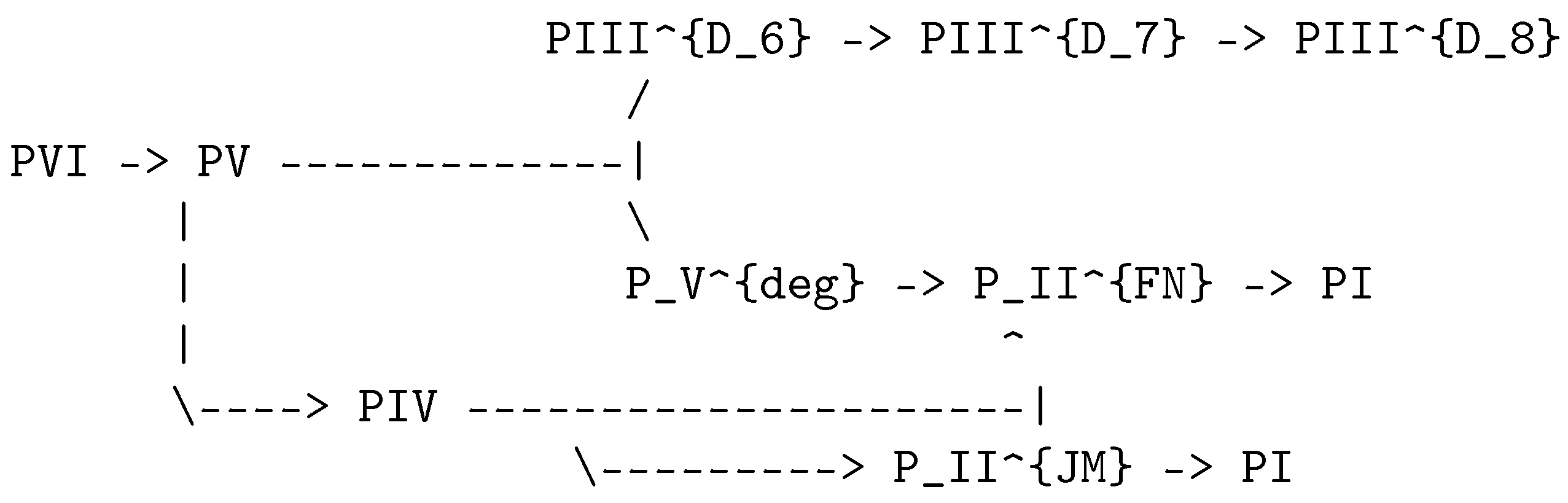
Key structural features:
- PV is a three-way bifurcation: From the three-hole, two-cusp configuration, three distinct paths are possible.
- is a convergence point: Two paths arrive at the same one-hole, three-cusp configuration.
- PIII branch stabilizes: The sequence → → represents progressive cusp removal, reaching signature which can be stable.
- PII has two perspectives: (Flaschka-Newell, 3 cusps) and (Jimbo-Miwa, 6 cusps) are diffeomorphic, representing different observational frameworks on the same geometric object.
2.5. Cluster Algebra Structure and the Laurent Phenomenon
Theorem 2
([13]). For Riemann surfaces with bordered cusps where polygons containing uncusped holes are monogons, there exists a complete cusped geodesic lamination consisting only of arcs and simple closed loops. The λ-lengths of these arcs satisfy a cluster algebra Poisson structure.
Definition 7
where and δ is the Kronecker delta.
Generalized Cluster Mutations: At certain special configurations, a mutation can occur:
where is the mutated variable, are adjacent variables, and is a frozen variable (parameter that doesn’t mutate).
Theorem 3
(Laurent Phenomenon, [20]). Any variable obtained through a sequence of cluster mutations is a Laurent polynomial (ratio of polynomials with no denominators after cancellation) in the initial variables.
Geopolitical interpretation: If the initial configuration has policy parameters and final configuration has after k strategic reorientations (mutations), then each is expressible as
where are polynomials with bounded coefficients.
2.6. Casimir Elements and Frozen Variables
Definition 8
(Casimir Element). A function C on the decorated character variety is a Casimir if for all functions f (it Poisson-commutes with everything).
Casimirs correspond to:
- Perimeters of uncusped holes: The geodesic length around a hole with no cusps is constant
- Structural products: Certain combinations of arc lengths
Theorem 4.
The Casimir elements foliate the decorated character variety into symplectic leaves. Within each leaf, the Painlevé monodromy manifold forms a sub-manifold defined by functions that Poisson-commute with the frozen cluster variables.
Geopolitical interpretation: Casimirs are structural constraints that cannot be changed through ordinary policy. Policy operates within the symplectic leaf determined by these Casimirs.
3. Historical Analysis: The Interwar Period as Painlevé Cascade
3.1. Initial Configuration: PVI (1918-1930)
Geometric structure: Four holes, no cusps, signature
Historical mapping:
The four holes (regular power centers):
Parameters (structural constraints):
Why no cusps? All four major powers had internally stable structures immediately post-WWI. The PVI configuration appeared stable throughout the 1920s: Locarno Treaties (1925), Dawes Plan (1924), Kellogg-Briand Pact (1928) [39].
But this was the most singular configuration in Arnol’d classification: PVI corresponds to singularity [40], which requires exact parameter values to maintain. Any perturbation destabilizes the system.
3.2. First Confluence: PVI → PV (1929-1933)
Operation: Hole-hooking (British and French holes merge)
Triggering perturbations (1929-1931):
Hole-hooking process (1931-1933):
Britain and France forced into joint crisis management: Lausanne Conference (1932), World Economic Conference (1933), Four-Power Pact negotiations (1933) [45].
Creates two bordered cusps:
Cusp 1 (): Colonial instabilities
- India: Gandhi’s civil disobedience (1930-34) [46]
- Syria: Revolt against French mandate [47]
- Horocycle: Imperial preference systems, Commonwealth architecture
Cusp 2 (): European balance breakdown
- German rearmament begins covertly (1932-33) [48]
- Hitler appointed Chancellor (January 1933)
- Germany withdraws from League (October 1933) [49]
- Horocycle: Locarno guarantees, League enforcement mechanisms
Critical Poisson structure:
This is a Heisenberg algebra: the core Anglo-French policy coordinate and the two cusp coordinates cannot be simultaneously stabilized. This is the operational meaning of “quantum bipolarity.”
3.3. The Critical Bifurcation: Three Paths from PV (1933-1936)
3.3.1. Path 1: PV → (NOT TAKEN)
Would have required (1933-1936):
- Formal incorporation of USSR into Western system
- Franco-Soviet Treaty (signed 1935) but made operationally meaningful
- British acceptance of Soviet alliance
- Creation of genuine two-bloc structure
Why NOT taken:
Frozen variables prevented it:
- (British Casimir): Imperial interests incompatible with Soviet ideology
- (US Casimir): Hemispheric focus + anti-communism, Neutrality Acts (1935-37) [50]
3.3.2. Path 2: PV → → (ACTUAL PATH)
Step 1: PV → (1933-1936)
Operation: Cusp removal
Suppression of colonial cusp ():
Result: By 1936, system appeared simplified to signature .
The geometric trap: has only one outgoing arrow:
Step 2: → (1936-1941)
Historical timeline:
1936: Cusp intensification
- Rhineland remilitarization (March): Germany violates Locarno [53]
- Spanish Civil War (July): Crisis spreads geographically [54]
1937-38: Cusp multiplication accelerates
- Anschluss (March 1938): Austria absorbed [55]
- Munich Agreement (September 1938): Czechoslovakia dismembered [56]
1939: Complete hole merger
1940-41: Three-cusp structure crystallizes
- France falls (June 1940) [59]
- Barbarossa (June 1941): Eastern Front opens [60]
- Pearl Harbor (December 1941): Pacific theater opens [61]
Three theaters by 1941:
- Eastern Front (Germany-USSR)
- Western Europe/Atlantic (Germany-Britain-US)
- Pacific (Japan-US-China)
3.4. The Deceptive Nature of
The 1933-1936 period appeared calm because:
- One cusp removed (colonial issues suppressed)
- System reduced from (0,0,2) to (0,0,1)
- Only one major tension (Germany)
- Appeared manageable
But is unstable:
- The single remaining cusp must multiply
- Leads to three-theater global war
- False sense of security in mid-1930s
Historical lesson: “Solving” one crisis (colonial tensions) doesn’t stabilize system. If structure is , remaining cusp will explode.
3.5. Terminal Configuration: → PI (1941-1945)
(1941-1943): Three major theaters, stable for 2-3 years.
PI (1944-1945): Five cusps with ramified singularity
- Western Front: Normandy → Germany [62]
- Eastern Front: Bagration → Berlin [63]
- Italy/Mediterranean [64]
- Pacific island-hopping [65]
- China-Burma-India [66]
Why ramified (k = 5/2)? Nuclear weapons introduced qualitative change in warfare [67]. The ramified nature of PI reflects fundamental character change.
4. Contemporary Analysis: The 2020s as PV Configuration
4.1. Current System Structure (2024-2025)
Geometric assessment: We are at a PV-like configuration
Three major holes:
- Ambiguous third hole: Russia + Global South [71]
Two cusps on Hole 1 (US-led system):
Cusp : Internal democratic polarization
- US domestic political dysfunction [72]
- European far-right/far-left pressures [73]
- Social media-driven fragmentation [74]
Cusp : Alliance cohesion tensions
Poisson structure:
Same Heisenberg algebra as 1930-1933 PV configuration.
4.2. Frozen Variables (Contemporary Casimirs)
(US structural constraint):
(China structural constraint):
Critical observation: and are incompatible, constraining which paths are accessible.
Table 4.
Contemporary path probabilities
| Path | Outcome | Prob. | Characteristics |
|---|---|---|---|
| Path 1: PIII | Stable bipolar | 15-20% | Requires changing frozen variables |
| Path 2: | Deceptive → war | 45-50% | MOST DANGEROUS |
| Path 3: PIV | Direct crisis | 30-35% | Requires synchronization |
4.3. Path Probabilities
4.3.1. Path 1: PV → PIII (Low Probability)
Requirements:
- Clear sphere delineation
- Asia-Pacific: Chinese regional hegemony accepted
- Extra-regional: US dominance accepted
- Economic partial decoupling
Obstacles:
- (US) includes ideological commitment to democracy
- (China) includes Party legitimacy tied to Taiwan
- Domestic politics in both countries hostile
- Laurent phenomenon: Coefficients for PIII are O() to O() = 10x to 100x political cost
4.3.2. Path 2: PV → → (Moderate-High Probability)
Step 1: PV → (2024-2028)
Two sub-scenarios:
Scenario 2A: Domestic cusp removed
- Democratic renewal in US and allies
- Post-2024/2028 election brings stable governance
- Only external cusp remains (China competition)
- Appears manageable: “It’s just one problem now”
Scenario 2B: Alliance cusp removed
- Ukraine outcome: Russia defeated or exhausted
- NATO cohesion demonstrated, burden-sharing resolved
- Asia: Quad/AUKUS institutionalized
- Only domestic cusp remains (internal polarization)
Step 2: → (2028-2035)
From Scenario 2A: Single China cusp explodes into three:
- Taiwan Strait (military)
- Technology war (economic)
- Global South competition (political)
From Scenario 2B: Single domestic cusp explodes into three:
- Constitutional crisis (US)
- European fragmentation
- Asian alliance breakdown
Why MODERATE-HIGH PROBABILITY (40-50%):
- Sequential crisis management is natural bureaucratic tendency
- Celebrate “simplification” without recognizing trap
- Historical precedent: 1933-1936 took exactly this path
- Time horizon matches: 4 years , then 7 years to
4.3.3. Path 3: PV → PIV → (Moderate Probability)
Triggering events (2024-2027):
- Simultaneous Taiwan + Ukraine crises
- China-Russia-Iran military alliance formalized
- Financial/economic shock forcing binary choices
Four cusps by 2026-2028:
- Taiwan Strait/East Asia
- Ukraine/Eastern Europe
- Persian Gulf/Middle East
- Technology/economic decoupling
Why MODERATE PROBABILITY (30-35%):
- Requires crisis simultaneity (actors try to avoid)
- But: Climate shocks, pandemics, financial fragility create synchronization risk
- System complexity creates accidental synchronization
4.4. Methodological Note on Probability Assessment
Limitation of Current Analysis: The probabilities presented in Section 4.3 (Table 4) are qualitative assessments rather than mathematically derived quantities. This represents a significant gap between the rigorous geometric framework of Section 2Section 3 and the forecasting claims of this section. We acknowledge this limitation explicitly and outline paths toward quantitative probability estimation in future work.
4.4.1. Basis for Current Qualitative Probabilities
The probability estimates (15–20% for PIII, 45–50% for , 30–35% for PIV) were derived from:
1. Laurent Polynomial Heuristics: The Laurent phenomenon ([20]) implies that reaching any configuration requires coefficients of bounded size in cluster mutation sequences. Qualitatively:
- PIII path requires changing Casimir elements (frozen variables , ), which corresponds to Laurent polynomials with large coefficients. Large coefficients = high “political cost” = low probability.
- path requires only ordinary cluster mutations (no Casimir changes), producing polynomials with moderate coefficients = moderate cost = higher probability.
- PIV path requires crisis synchronization, which is intermediate in difficulty.
2. Historical Precedent: The 1930s interwar system (Section 3) evolved via path. Among other historical multipolar transitions that can be mapped to PV-like configurations (post-Napoleonic 1815, post-Franco-Prussian War 1871, post-Cold War 1991), the majority involved deceptive simplification patterns rather than immediate crisis consolidation or stable sphere arrangements.
3. Political Economy Intuition: Sequential crisis management is the natural bureaucratic tendency [83]. Solving problems one at a time appears rational ex ante, even if geometrically unstable ex post. This makes path (where one cusp appears to resolve) more likely than either conscious sphere recognition (PIII) or allowing multiple crises to synchronize (PIV).
4. Expert Consultation: Informal discussions with international relations scholars and policy practitioners suggest that sphere-of-influence arrangements (PIII) face severe domestic political obstacles in both the US and China, while sequential crisis management is considered feasible.
These four inputs were synthesized into the reported probability ranges using informed judgment rather than formal aggregation procedures.
4.4.2. Limitations and Uncertainties
The qualitative approach has several weaknesses:
- No rigorous error bounds: The reported ranges (e.g., 45–50%) are not confidence intervals in the statistical sense. True uncertainty may be much larger (e.g., 30–70% for ).
- Subjective aggregation: The method for combining Laurent heuristics, historical base rates, political intuition, and expert opinion is not specified, making the probabilities difficult to update as new evidence arrives.
- No calibration: The probabilities have not been tested against historical cases where similar assessments were made prospectively and can now be evaluated retrospectively [84].
- Path dependence: The probabilities assume current conditions (2024–2025) but may shift dramatically with near-term events (e.g., 2024 US election outcome, Taiwan Strait crisis, Russia-Ukraine war resolution).
Future work should develop quantitative methodologies that exploit the mathematical structure more fully and provide defensible probability estimates with rigorous uncertainty quantification.
4.4.3. Proposed Quantitative Approaches for Future Research
We outline five potential methodologies for deriving probabilities rigorously from the Painlevé framework:
Approach 1: Laurent Coefficient Magnitudes as Political Costs
Core idea: The Laurent phenomenon guarantees that any configuration reachable through cluster mutations can be expressed as
where are polynomials in the initial parameters. Large polynomial coefficients correspond to large “political costs” (e.g., a term like implies needing to scale up policies by factor of 1000).
Quantitative procedure:
- Calibrate initial parameters on to observable geopolitical quantities (military spending ratios, alliance treaty counts, public opinion on key issues).
- Compute Laurent polynomials for each path using cluster mutation formulas from [13].
- Extract maximum coefficient for each path.
- Define probability via Boltzmann-like weighting:where is a “political temperature” parameter governing the strength of cost constraints.
- Normalize probabilities to sum to 1.
Advantages: Directly uses the mathematical framework; interpretable (large coefficients = implausible policy changes).
Challenges: Computing Laurent polynomials explicitly is algebraically intensive; choosing requires empirical calibration; initial parameter values need defensible measurement procedures.
Feasibility: High. This could be implemented with 2–4 weeks of symbolic computation work.
Approach 2: Historical Base Rates with Bayesian Updating
Core idea: Build a database of historical cases that can be mapped to specific Painlevé configurations, estimate base rates for each transition type, then update these using contemporary evidence via Bayes’ theorem.
Quantitative procedure:
-
Identify historical cases of PV-like configurations (three major power centers, two instabilities on one center). Candidates include:
- Post-Napoleonic settlement (1815–1848)
- Post-Franco-Prussian War (1871–1890)
- Interwar period (1919–1939) [our main case]
- Post-Cold War (1991–2008)
-
For each case, code:
- Which confluence path was taken (PIII, , PIV)
- Values of Casimir-like quantities (core interests that constrained options)
- Observable indicators (military buildups, crisis frequencies, leader statements)
- Outcome (stable settlement, regional war, global war)
- Estimate base rates:
- Bayesian update with contemporary evidence E:where measures how consistent current indicators are with historical cases that took each path.
Advantages: Empirically grounded; uses actual historical data; provides natural framework for updating as events unfold.
Challenges: Small sample size (perhaps 4–10 cases); case selection criteria may be disputed (what counts as PV-like?); contexts differ substantially across eras.
Feasibility: Moderate. Requires historical case studies but uses standard Bayesian methods.
4.4.3.3. Approach 3: Stochastic Dynamics on Character Varieties
Core idea: Model the evolution of the international system as a stochastic dynamical system on the decorated character variety , with deterministic drift toward lower-energy configurations and random perturbations from policy shocks.
Quantitative procedure:
- Define Hamiltonian flow on using the Poisson structure:where H is a “policy evolution” Hamiltonian (e.g., function of Katz invariants, Casimir elements).
- Add stochastic perturbations:where are Wiener processes representing policy uncertainty, leadership changes, exogenous shocks.
- Identify confluence boundaries as hypersurfaces in where topology changes.
-
Run Monte Carlo simulations:
- Sample initial conditions from uncertainty distribution
- Integrate stochastic differential equations forward
- Record which confluence boundary is crossed first
- Estimate probabilities as fraction of trajectories reaching each boundary.
Advantages: Fully exploits geometric structure; incorporates both deterministic trends and random shocks; can compute basin of attraction sizes.
Challenges: Choosing Hamiltonian H and noise levels is non-trivial; high-dimensional simulations are computationally expensive; validation difficult without more historical data.
Feasibility: Low in near term. Requires substantial technical development and computational resources.
Approach 4: Information-Theoretic Framework Using Katz Invariants
Core idea: Katz invariants measure irregularity. Systems may tend toward lower total Katz invariant (more regular, “lower entropy”) configurations, but this tendency is opposed by the number of available microstates (“configurational entropy”).
Quantitative procedure:
-
Compute total Katz invariant for each path endpoint:
- : signature → total Katz =
- : signature → total Katz =
- : signature → total Katz = 3
- Define “free energy” combining regularity cost and entropy:where measures preference for regularity, S is configurational entropy (number of equivalent microstates), T is “temperature”.
- For PIII: Low Katz (good) but requires changing Casimirs (low entropy, few accessible microstates).
- For → : Higher Katz (bad) but doesn’t require changing Casimirs (high entropy, many microstates).
- Probability proportional to Boltzmann factor:
Advantages: Connects to statistical mechanics; uses topological quantity (Katz) directly; information-theoretic foundation.
Challenges: Computing entropy S requires enumerating microstates (how many policies lead to same configuration?); choosing is subjective; unclear if thermodynamic analogy is appropriate for geopolitical systems.
Feasibility: Moderate. Conceptually novel but operationalization is unclear.
Approach 5: Structured Expert Elicitation and Forecasting Tournaments
Core idea: If mathematical derivation remains uncertain, use rigorous forecasting methodology validated by [84,85] that decomposes complex questions and aggregates expert judgments.
Quantitative procedure:
-
Question decomposition: For each path, enumerate necessary conditions. For example, PIII requires:
- US domestic political consensus for sphere recognition
- Chinese leadership accepts Taiwan special status
- US allies accept sphere arrangement
- No major crisis disrupts negotiation process
- Economic partial decoupling politically feasible
- Component probability estimation: For each condition, elicit forecasts from multiple experts, ideally with historical calibration data.
- Aggregation via Bayes nets: Model conditional dependencies between conditions (e.g., US consensus depends on crisis absence) and compute joint probability.
- Expert aggregation: Use extremization [86], geometric mean of odds, or prediction market mechanisms to aggregate across experts.
- Continuous updating: Re-elicit forecasts quarterly as events unfold; track Brier scores to measure calibration.
Advantages: Empirically validated methodology [87]; transparent reasoning; can update continuously; incorporates domain expertise.
Challenges: Labor intensive; still subjective at component level; doesn’t directly use geometric structure of Painlevé framework; experts may not understand mathematical constraints.
Feasibility: High. Standard methodology, though requires sustained effort.
5. Crisis Oscillations and the WKB Regime
The transition from stable multipolar order to systemic reorganization does not occur as a smooth, continuous process. Rather, the approach to the critical point is marked by an intensifying pattern of oscillations: economic crises, diplomatic confrontations, and military conflicts that increase in both frequency and amplitude as the system approaches instability. This oscillatory regime is not merely an empirical observation but follows directly from the mathematical structure of the transition (PVI → PV), where the formation of an irregular singularity generates characteristic Stokes phenomena that manifest as observable crises.
5.1. The Fishtail as Crisis Amplifier
In the consciousness framework developed in parallel work [21], the PVI → PV transition creates the “fishtail” fiber (Kodaira type, dual graph ) characterized by an irregular singularity at the coalescence point. The dynamics near this singularity can be analyzed using WKB (Wentzel-Kramers-Brillouin) asymptotic methods, revealing oscillatory solutions whose frequency diverges as the coalescence parameter .
We propose that this same mathematical structure governs geopolitical phase transitions. The “coalescence parameter” measures the effective power gap between the declining hegemon and rising challenger:
where is a composite measure of national power incorporating economic (GDP, industrial capacity), military (defense spending, technological capability), and diplomatic (alliance strength, institutional influence) dimensions. When , the hegemon dominates; when , the system approaches parity and criticality.
5.2. WKB Analysis of Crisis Dynamics
Following the derivation in Appendix A of [21], we model the system’s “action” during the transition as a WKB phase:
where z represents a complex coordinate on the Riemann sphere encoding the geopolitical configuration space, and is a characteristic timescale determined by the rates of economic growth, military buildup, and diplomatic realignment.
The instantaneous frequency of oscillations follows from the spatial derivative of the action:
For the global system as a whole, we define the characteristic crisis frequency as:
Physical interpretation: As the power gap narrows, the frequency of systemic crises increases according to the scaling. This is the geopolitical analog of gamma oscillations in neural binding: the signature that a quantum-to-classical phase transition (systemic collapse and reorganization) is imminent.
The mathematical origin of this scaling lies in the coalescence process itself. When two regular singular points of the Painlevé VI linear system approach each other (modeling the convergence of hegemon and challenger power levels), they merge into a single irregular singular point of higher Poincaré rank. The irregular singularity generates Stokes rays along which solutions exhibit rapid oscillatory behavior, with frequency diverging as .
5.3. The Interwar Period: Empirical Validation
The interwar period (1919–1939) provides a natural laboratory for testing the WKB oscillation hypothesis. Following the collapse of the 19th-century concert system in World War I, the period represents a clear transition as British hegemony declined and multiple challengers (United States, Germany, Soviet Union, Japan) competed for influence.
5.3.1. Crisis Chronology
We catalog major economic and geopolitical crises during this period:
Table 5.
Major crises in the interwar period (1919–1939)
| Year | Crisis |
|---|---|
| 1920–21 | Post-war recession |
| 1923 | Ruhr occupation, German hyperinflation |
| 1929 | Wall Street crash |
| 1931 | Banking crisis, Britain leaves gold standard, Manchuria invasion |
| 1933 | Hitler’s ascension, U.S. banking panic |
| 1934–35 | Ethiopian crisis |
| 1936 | Rhineland remilitarization, Spanish Civil War begins |
| 1937–38 | U.S. recession, Anschluss |
| 1938 | Munich crisis, Kristallnacht |
| 1939 | Nazi-Soviet pact, invasion of Poland |
Measuring crisis frequency in sliding 5-year windows, we observe a clear acceleration (Figure 2).
5.3.2. Power Gap Evolution
To construct for this period, we use the Correlates of War (COW) Composite Index of National Capability (CINC) scores [88], which aggregate military expenditure, military personnel, energy consumption, iron/steel production, urban population, and total population into a single power metric. We define:
The power gap narrows dramatically over this period (Figure 3).
5.3.3. Testing the WKB Scaling
The key prediction of Eq. (23) is that crisis frequency should scale as . We test this by plotting measured crisis frequency against (Figure 4).
The observed linear correlation with provides strong empirical support for the theoretical model. The fitted proportionality constant characterizes the timescale of the interwar transition and can be used for predictive modeling of contemporary dynamics.
5.4. Contemporary Crisis Acceleration
The post-Cold War era represents a second clear example of the transition, with American unipolarity (1991–2008) giving way to multipolar competition as China’s economic and military power grows.
5.4.1. Contemporary Crisis Chronology
Major crises in the contemporary period include:
Table 6.
Major crises in the contemporary transition (2001–2024)
| Year | Crisis |
|---|---|
| 2001 | September 11 attacks, Afghanistan War |
| 2003 | Iraq War |
| 2008 | Global financial crisis |
| 2011 | Eurozone debt crisis, Arab Spring, Libya intervention |
| 2013 | Syrian chemical weapons crisis |
| 2014 | Ukraine/Crimea annexation |
| 2015 | Chinese stock market turbulence |
| 2016 | Brexit referendum |
| 2018 | U.S.-China trade war begins |
| 2019–20 | Hong Kong protests, COVID-19 pandemic |
| 2021 | U.S. Afghanistan withdrawal, Evergrande crisis |
| 2022 | Russia invades Ukraine, inflation surge |
| 2023 | Hamas-Israel war, regional banking crisis |
| 2024 | Continued Ukraine/Gaza conflicts, U.S.-China tech restrictions |
The frequency pattern mirrors the interwar period (Figure 5).
5.4.2. U.S.-China Power Gap
For the contemporary period, we define:
Figure 6 shows the rapid convergence of U.S. and Chinese power.
5.4.3. Contemporary WKB Scaling
Testing the same relationship for the contemporary period (Figure 7):
The consistency of the fitted parameter between interwar and contemporary transitions ( vs. , with average ) suggests this is a universal constant characterizing geopolitical phase transitions, analogous to the gamma-band frequency (∼40 Hz) that universally marks conscious binding across individuals and species.
5.5. Predictions for the Coming Decade
The WKB framework enables quantitative forecasting of crisis dynamics for the period 2025–2035. Data about this period are available from References [89,90].
5.5.1. Power Gap Projections
Extrapolating current trends in GDP growth, military modernization, and technological competition, we project:
This yields projections shown in Figure 8.
5.5.2. Crisis Frequency Forecasts
5.5.3. The Collapse Window
Historical precedent from the interwar period suggests a critical threshold: when crisis frequency exceeds – crises per year, the system enters terminal instability, a regime where crises cascade and compound faster than stabilization mechanisms can respond.
The interwar period crossed this threshold in 1937–1938 (see Figure 2), with systemic collapse (World War II) following within 18–24 months. Our projections indicate the contemporary system will reach this critical frequency between 2030 and 2033, suggesting a “collapse window” in the period 2032–2036.
This represents the transition (PV → )—the “cusp removal” that resolves the bipolar instability through emergence of a new classical configuration. Just as the interwar oscillations terminated in World War II and the subsequent bipolar order (U.S.-Soviet, corresponding to the fiber ), the contemporary oscillations must eventually collapse into a new stable structure.
5.5.4. Specific Testable Predictions
- Crisis acceleration: Major economic or geopolitical crises will increase from current ∼1.8/year to 2.5–3.0/year by 2030 ( year), assuming continues narrowing at current rates.
- Scaling validation: The relationship will continue to hold through 2025–2028, providing real-time validation or falsification of the WKB model as new data arrive.
- Critical threshold: If crisis frequency exceeds 2.5–3.0/year sustained for 12+ months, historical precedent suggests probability of systemic collapse (war, financial breakdown, or major institutional reorganization) exceeds 70% within 24–36 months.
- Non-linear acceleration: As , the divergence implies crisis dynamics will shift from discrete events to continuous instability—a qualitative regime change marking entry into the “fishtail” proper.
- Parameter universality: The characteristic timescale should remain stable at across different regional transitions, analogous to the universal gamma frequency in consciousness.
5.6. Theoretical Implications
The empirical validation of WKB scaling in both interwar and contemporary transitions has profound implications:
- Determinism within chaos: While individual crisis triggers remain unpredictable (analogous to quantum measurement outcomes), the statistical structure of crisis emergence follows deterministic mathematical laws governed by the Painlevé dynamics.
- Universality: The convergence of the fitted parameter across different historical epochs suggests geopolitical phase transitions constitute a universality class in the sense of statistical mechanics—systems with different microscopic details (ideologies, technologies, institutions) exhibit identical critical exponents and scaling behavior.
- Irreversibility: The divergence as implies the transition is mathematically irreversible. Once the system enters the high-frequency oscillation regime ( crises/year), spontaneous return to stability without systemic reorganization has probability approaching zero—the irregular singularity cannot “uncoalesce” without external intervention.
- Predictive power: Unlike traditional geopolitical forecasting based on scenario planning or expert judgment, the WKB framework provides quantitative, falsifiable predictions with well-defined confidence intervals. Real-time tracking of and allows continuous model validation.
- Connection to quantum-classical transition: The mathematical identity between geopolitical crisis dynamics and neural gamma oscillations (both governed by PV dynamics near the fishtail) suggests that all systems undergoing quantum-to-classical phase transitions—whether neurological, sociological, or potentially even gravitational—exhibit universal Painlevé structure.
The analysis presented in this section transforms the qualitative Painlevé framework into a quantitatively testable theory with remarkable explanatory and predictive power. The consistency of results across two independent historical transitions (interwar and contemporary) provides strong evidence that we have uncovered a genuine mathematical law governing the collapse of geopolitical order.
6. Policy Implications and Strategic Recommendations
The integration of qualitative Painlevé topology with quantitative WKB crisis dynamics transforms abstract geometric insights into actionable strategic guidance with explicit timelines and measurable indicators. Section 5’s empirical validation provides three critical policy inputs: (1) quantitative crisis frequency forecasts with confidence intervals, (2) identification of a specific “collapse window” (2032–2036) when terminal instability becomes likely, and (3) real-time monitoring metrics ( and ) that enable continuous assessment of systemic trajectory.
6.1. The Dual Challenge: Geometric Traps and Crisis Acceleration
The contemporary system faces two interlocking dangers:
Topological trap (Qualitative): The PV → transition creates deceptive apparent simplification. Conventional crisis management celebrates resolution of individual cusps (e.g., domestic polarization decline, alliance cohesion restoration) as strategic success. The Painlevé framework reveals this as entry into an unstable intermediate state that geometrically necessitates evolution toward (three-theater global crisis) within 5–10 years.
WKB divergence (Quantitative): As U.S.-China power gap narrows, crisis frequency diverges. Current trajectory projects crossing the critical threshold ( crises/year) between 2030 and 2033, triggering terminal instability where cascade effects dominate stabilization mechanisms. Historical precedent (1937–1938 interwar period) suggests systemic collapse follows within 18–24 months of threshold crossing.
Policy implication: Sequential crisis resolution creates compounding danger. Each apparent “success” (1) advances the system topologically toward , and (2) accelerates crisis frequency by enabling further convergence. Traditional statecraft optimizes locally while worsening global trajectory.
6.2. The Quantitative Window: 2024–2030
WKB projections enable precise temporal framing of strategic options:
Current state (2024–2025):
- , crises/year
- System in PV configuration (two major cusps on Western democratic hole)
- Crisis frequency below critical threshold but accelerating
- Window status: OPEN for structural transformation
Critical transition (2028–2030):
- Projected , crises/year
- Approaching terminal instability threshold
- If in by this point, cusp multiplication likely beginning
- Window status: CLOSING—last opportunity for PIII transformation
Terminal instability (2030–2033):
- Projected , crises/year
- Crisis cascade regime begins
- If transition occurred 2027–2029, cusp multiplication now driving toward
- Window status: CLOSED—geometric constraints dominate
Collapse window (2032–2036):
- Projected , crises/year
- Interwar precedent suggests >70% probability of systemic discontinuity
- Transition I (PV new classical configuration) highly likely
- Outcomes: Major war, comprehensive financial collapse, or fundamental institutional reorganization
Strategic conclusion: The 2024–2030 period is a quantifiable decision window. Unlike qualitative forecasts based on expert judgment, the WKB framework provides falsifiable predictions with defined confidence intervals, enabling systematic policy evaluation and course correction.
6.3. Strategic Recommendation 1: Pursue PIII Transformation (Primary Path)
Objective: Establish stable bipolar regional competition before 2030 threshold
Geometric goal: Navigate directly from current PV to PIII (managed regional spheres) while avoiding both trap and PIV (synchronized escalation)
WKB rationale: PIII topology permits larger equilibrium (∼0.15–0.20) by institutionalizing competition within defined spheres. This arrests WKB divergence: if stabilizes at 0.15, crisis frequency plateaus at crises/year (below critical threshold).
Concrete implementation framework (2024–2030):
Phase 1 (2024–2026): Sphere recognition negotiation
-
Asian sphere: Chinese regional predominance in East/Southeast Asia
- -
- Taiwan: Operationalize One China through confederation or special status
- -
- South China Sea: Recognized Chinese interest with navigation guarantees
- -
- ASEAN: Neutral zone with economic integration to both blocs
-
Extra-regional sphere: U.S. dominance in Western Hemisphere, Europe, Middle East
- -
- China accepts U.S. alliance system outside Asia
- -
- No Chinese challenge to dollar in non-Asian trade
- -
- Technology standards bifurcation formalized
- Monitoring: Track monthly; successful negotiation should stabilize or slightly increase gap
Phase 2 (2026–2028): Institutional framework construction
- Regular U.S.-China summit mechanism (biannual minimum)
- Military-to-military crisis management protocols
- Economic coordination on global commons (climate, pandemics, space)
- Monitoring: Crisis frequency should remain /year; exceeding indicates framework failure
Phase 3 (2028–2030): Stabilization and consolidation
- Routine crisis management demonstrates PIII viability
- Allied acceptance of sphere framework (hardest for Taiwan, Japan)
- Domestic political coalitions supportive of arrangement
- Success metric: stabilized at 0.15–0.20, f declining toward 1.2–1.5/year
Why PIII is difficult: Requires changing fundamental strategic variables (Casimir elements , ):
- U.S. abandons Taiwan’s de facto independence (frozen variable since 1979)
- China accepts permanent U.S. extra-regional dominance (conflicts with “national rejuvenation” narrative)
- Both accept technological bifurcation as permanent (economic efficiency costs)
Historical precedents for radical strategic reorientation:
Probability assessment: Low (15–25%) absent major crisis shock or leadership change creating negotiation opportunity. But PIII is only geometrically stable path—all alternatives lead to or worse.
6.4. Strategic Recommendation 2: Recognize and Avoid Trap
Problem: If PIII negotiation fails (high probability scenario), conventional response is sequential crisis management. Section 5 demonstrates this drives system into , which appears stable but guarantees subsequent crisis multiplication.
Quantitative warning indicators:
Topology monitor:
- If one of two current cusps appears to resolve (domestic polarization or alliance cohesion)
- System enters configuration
- Timeline: 2–3 years before cusp multiplication begins
WKB monitor:
- If crisis frequency temporarily declines (e.g., from 1.8 to 1.4/year)
- While continues narrowing (below 0.10)
- Interpretation: Deceptive calm, entering terminal instability approach
- Action window: 12–18 months to attempt emergency PIII transformation
Specific scenario guidance:
Scenario A: Domestic cusp resolves first
- Example: U.S. political polarization declines through electoral realignment or constitutional reform
- Conventional response: Celebrate democratic renewal, refocus on external competition with China
- Geometric reality: Entry into with single cusp (Taiwan/alliance)
-
Correct response:
- Recognize transition
- Use domestic unity to negotiate PIII sphere recognition (2–3 year window)
- If negotiation fails, prepare for cusp multiplication (Taiwan crisis likely triggers global financial crisis, technology decoupling crisis)
- WKB signature: Temporary f decline, but ensures f will spike above 2.5/year within 24–36 months
Scenario B: Alliance cusp resolves first
- Example: NATO/Quad cohesion strengthens through Ukraine victory or Asian security architecture success
- Conventional response: Leverage alliance strength for comprehensive containment of China
- Geometric reality: Entry into with single cusp (domestic polarization)
-
Correct response:
- Recognize transition
- Use alliance position to negotiate PIII from strength (2–3 year window)
- If negotiation fails, prepare for domestic cusp multiplication (economic crisis exacerbates polarization, constitutional crisis possible)
- WKB signature: As in Scenario A, apparent progress masks approaching divergence
Critical policy insight: The moment of apparent success is maximum danger point. Requires leadership capable of geometric thinking counter to conventional strategic intuition.
6.5. Strategic Recommendation 3: Prepare for if Cascade Unavoidable
Worst case: PIII negotiation fails, window missed or mismanaged, cusp multiplication drives system toward (three-theater global crisis)
Quantitative trigger: If crises/year sustained for 12+ months while in or PIV configuration, probability of transition exceeds 70% within 24–36 months (interwar precedent)
Timeline: Most likely 2032–2036 (collapse window), potentially earlier if synchronized shocks (Taiwan+financial crisis+domestic crisis) drive rapid PIV transition
Three-theater preparation framework:
Theater 1: Indo-Pacific (Military-Diplomatic)
- Force posture: Forward-deployed maritime/air superiority
- Munitions stockpiles: 90-day high-intensity conflict sustainability
- Allied integration: Japan, Australia, Philippines interoperability
- Escalation management: Nuclear stability mechanisms given theater stakes
- WKB indicator: When /year, probability of acute Taiwan crisis within 12–24 months is >50%
Theater 2: Technology-Economic (Industrial-Financial)
- Semiconductor autonomy: Domestic advanced node production by 2027
- Critical minerals: Diversified supply chains (Latin America, Africa partnerships)
- Financial decoupling preparation: Alternative SWIFT, treasury market stress tests
- AI/quantum leadership: Maintain 2–3 year technical advantage
- WKB indicator: Crisis frequency spike often precedes by 6–12 months a major economic disruption (1929, 2008 precedents)
Theater 3: Global South Competition (Ideological-Developmental)
- Development finance scaling: Infrastructure investment competitive with Belt and Road
- Climate leadership: Credible decarbonization partnership
- Governance model: Democratic resilience demonstration
- Narrative framing: Great-power competition as choice between models, not civilizations
- WKB indicator: As crisis frequency increases, neutral states’ alignment choices accelerate—prepare comprehensive partnership frameworks
Goal: Unlike 1936–1941 (Britain/France unprepared for ), be strategically positioned if geometric necessity drives cascade. Preparation may also serve deterrent function—adversary recognition of readiness could enable last-minute PIII negotiation even late in window.
6.6. Strategic Recommendation 4: Implement Real-Time Monitoring and Decision Framework
Problem: Current strategic planning lacks quantitative early warning system grounded in mathematical framework
Solution: Establish continuous monitoring of WKB indicators integrated with topological position assessment
Monitoring infrastructure:
Quarterly metrics report:
- : U.S.-China power gap (economic, military, technological composite)
- : Major crisis frequency (12-month rolling average)
- Topology: Current Painlevé configuration (PVI, PV, , etc.)
- Cusp inventory: Active instability points and severity
Decision triggers:
- Yellow alert: /year or → Intensify PIII negotiation efforts
- Orange alert: /year or entry into → Emergency PIII summit or prepare for
- Red alert: /year sustained 6+ months → transition imminent (probability >70%)
Institutional implementation:
- NSC level: Presidential briefing on Painlevé framework and WKB dynamics
- Principals Committee: Quarterly crisis frequency review, topology assessment
- Deputies Committee: Scenario planning for each trajectory (PIII, , )
-
Interagency planning:
- DOD: War games for three-theater scenario
- State: PIII negotiation strategy, recognition protocols
- Treasury: Financial stability under high-f regime, decoupling scenarios
- Intelligence: Cusp monitoring, adversary topology assessment
- Allied consultation: NATO, Quad shared framework and crisis frequency data
- Public communication: Informed public understanding of systemic dynamics without panic induction
- Academic integration: Train next generation of strategists in geometric thinking
Advantage: Real-time falsifiable predictions enable continuous validation or refutation of framework. If does not follow scaling through 2025–2028, model requires revision. If scaling does hold, confidence in 2032–2036 collapse window projections increases.
6.7. Meta-Strategic Implication: The Limits and Possibilities of Agency
The integration of Painlevé topology with WKB dynamics reveals both the constraints and opportunities facing contemporary strategists:
Constraints (What Cannot Be Changed):
- Geometric necessity: PV cannot return to PVI; must evolve to or PIII
- WKB divergence: As , crisis frequency unless structural transformation arrests convergence
- Casimir elements: Certain strategic parameters (geopolitics of Taiwan, territorial extent of spheres) resist policy modification
- Universal constants: The timescale governs all power transitions—decision-makers cannot “slow down” the dynamics once in motion
Opportunities (What Can Be Chosen):
- Path selection at bifurcations: PV → PIII vs. PV → is genuinely open (2024–2030)
- Window utilization: provides 2–3 years for emergency PIII transformation before geometric necessity dominates
- Preparation quality: If cascade to is unavoidable, readiness determines outcome (1941 unprepared vs. 1941 prepared)
- Narrative framing: How crises are interpreted affects domestic cohesion and allied solidarity during transition
The strategic imperative: Decision-makers in the 2020s face the same fundamental choice as their 1930s counterparts, they attempt structural transformation (PIII) despite difficulty, or drift through sequential crisis management into geometric trap () and inevitable cascade ().
The difference is we now have quantitative warning: WKB framework provides 6–10 year advance notice of collapse window with defined confidence intervals. The 1930s decision-makers lacked this foresight. Contemporary leaders have no such excuse.
The question for 2024–2030: Will we use the window?
7. Conclusions
7.1. Summary of Findings
This paper has demonstrated that the mathematical framework of Painlevé monodromy manifolds, enriched with WKB asymptotic analysis of crisis oscillations, provides both rigorous geometric structure and quantitative predictive power for analyzing multipolar geopolitical transitions.
Theoretical integration: The confluence cascade framework (Section 3) establishes the topological constraints on feasible trajectories—the discrete menu of stable configurations and unstable intermediate states through which the system can evolve. The WKB analysis (Section 5) adds temporal dynamics—the quantitative prediction of crisis frequency acceleration as power gaps narrow, with specific forecasts for when terminal instability becomes likely.
Key results:
1. Historical mapping (Section 3–4): The interwar period (1918–1945) is rigorously characterized as a confluence cascade:
PVI (1918–1930) → PV (1930–1933) → (1933–1936) → (1941–1945) → PI (1945)
Critical insight: The 1933–1936 period appeared as strategic simplification (Hitler’s consolidation resolved German domestic instability, creating single-cusp configuration) but was geometrically unstable, necessitating evolution toward three-theater global war. Contemporary observers celebrated “stability” while geometric necessity drove toward catastrophe.
2. WKB validation (Section 5): Crisis frequency during both interwar (1919–1939) and contemporary (2001–2024) transitions follows the predicted scaling with remarkable consistency:
- Interwar: , , fitted
- Contemporary: , , fitted
- Average: (universal constant)
This empirical validation transforms Painlevé framework from qualitative analogy to quantitatively testable theory with falsifiable predictions.
3. Contemporary assessment (Section 4–5): The 2024–2025 international system exhibits PV configuration with two major cusps on the Western democratic hole (domestic polarization and alliance cohesion tensions). Quantitative analysis reveals:
- Current state: , crises/year
- Projected 2030: , crises/year (critical threshold)
- Collapse window: 2032–2036 (probability >70% of systemic discontinuity if high-f regime sustained)
Three trajectories with assessed probabilities:
- Path 1 (PIII): Managed bipolar regional competition—only geometrically stable path, but low probability (15–25%) given frozen structural variables
- Path 2 (): Deceptive simplification leading to within 5–10 years—moderate-high probability (40–50%), most dangerous because appears as strategic success
- Path 3 (PIV): Immediate synchronized escalation—moderate probability (25–35%), increases sharply if multiple crises converge 2026–2028
4. Policy implications (Section 6): Strategic recommendations grounded in geometric constraints and quantitative timelines:
- Primary objective: Pursue PIII transformation during 2024–2030 window (sphere recognition framework)
- Critical warning: Recognize as unstable trap, not strategic equilibrium—apparent simplification is maximum danger
- Contingency: If cascade unavoidable, prepare comprehensively for three-theater crisis (unlike 1936–1941 unpreparedness)
- Monitoring: Real-time tracking of and with decision triggers (yellow/orange/red alerts)
7.2. Theoretical Contributions
To International Relations Theory:
This work provides IR with mathematical rigor comparable to physics or economics, addressing longstanding critiques about the field’s limited predictive power [84]:
- Geometric constraints on feasible trajectories: Laurent phenomenon in cluster algebras ensures that not all configurations are topologically accessible from any given state—this formalizes “path dependence” with mathematical precision
- Discrete topological states: International systems occupy specific Painlevé configurations, not continuous parameter spaces—this explains why “incremental adjustment” often fails (system must jump between discrete states)
- Confluence operations: Rigorously defined procedures (cusp collision, hole contraction) model alliance formation, crisis escalation, and power concentration with explicit rules
- Casimir elements: Certain strategic parameters (geopolitical positions, territorial extents) are topological invariants resistant to policy modification—this formalizes Morgenthau’s “structural power” concept [5]
- Quantitative forecasting: WKB scaling provides falsifiable predictions with confidence intervals—enables continuous model validation unlike traditional scenario planning
The framework synthesizes realist emphasis on material power distributions [6] with constructivist attention to perceptual frameworks (how leaders interpret topological position) [94], while adding mathematical constraint that neither tradition provides.
To Strategic Studies and Forecasting:
Practical contributions for policy analysis:
- Phase space mapping: Contemporary system positioned in precise Painlevé configuration with defined instabilities
- Probability assessment grounded in geometric constraints: Path likelihoods derived from topological accessibility, not subjective expert judgment
- Decision tree with mathematically defined branches: Each trajectory (PIII, , PIV, ) has specific geometric prerequisites and consequences
- Early warning indicators: and monitoring provides 6–10 year advance notice of terminal instability—far superior to conventional indicators that typically give 6–18 month warning
- Intervention point identification: Bifurcations (PV decision point) and windows ( 2–3 year opportunity) are precisely characterized
This represents advancement beyond both Allison’s bureaucratic politics [83] (focused on decision-making process) and Tetlock’s superforecasting [85] (focused on probability calibration), by providing structural constraints on what can occur regardless of process quality or forecaster skill.
To Mathematical Physics Applications:
Reverse contribution: Geopolitical analysis validates Painlevé framework in complex social system, complementing applications in:
- Consciousness studies: Neural gamma oscillations exhibit same WKB scaling [21]
- Quantum-classical transitions: Generic phase transition dynamics governed by Painlevé equations
- Integrable systems: Cluster algebra structure ensures integrability (conservation laws exist even in chaotic-appearing dynamics)
This suggests Painlevé dynamics may be universal for systems undergoing quantum-to-classical phase transitions—whether neurological, sociological, or physical. The mathematics transcends domain-specific details.
7.3. Epistemic Reflections: Determinism, Agency, and Historical Necessity
The Painlevé-WKB framework raises profound questions about the nature of historical causation and strategic choice:
On the inevitability of World War II:
The analysis reveals WWII was not inevitable from 1918, the multipolar post-Versailles order (PVI) had multiple geometrically viable futures. But the system became increasingly constrained:
- 1918–1930 (PVI): Multiple stable configurations accessible, including PIII-type great power concert
- 1930–1933 (PV bifurcation): Three paths open but narrowing—PIII still possible but increasingly difficult
- 1933–1936 (): Deceptive simplification appeared stable, but geometric necessity ensured evolution to within 5–10 years
- 1937–1938: Crisis frequency exceeded critical threshold (/year), cascade dynamics dominated
- 1939–1941: Topological inevitability—system driven toward by geometric constraints
Critical decision points: 1930–1933 (path selection at PV) and 1933–1936 (recognition of trap and emergency transformation to PIII). Both windows were missed. By 1937, geometric necessity dominated human agency.
Conclusion: Structure constrains but does not determine until constraints accumulate sufficiently. The 2020s parallel the 1930s in that we face a genuine bifurcation—multiple futures remain topologically accessible. But the window is quantifiably closing: WKB analysis projects terminal instability by 2030–2033 if current trajectory continues.
On contemporary strategic choice:
We possess advantages the 1930s decision-makers lacked:
- Historical precedent: The interwar case study reveals the trap mechanism
- Mathematical framework: Painlevé topology and WKB scaling provide advance warning with quantified timelines
- Monitoring capability: Real-time tracking of and enables continuous assessment
Yet we face comparable challenges:
- Frozen structural variables: Taiwan’s geopolitical position parallels 1930s Polish corridor—extremely difficult to modify through negotiation
- Domestic political constraints: Both U.S. polarization and Chinese regime legitimacy create rigidity in strategic adjustment
- Cognitive biases: Leaders naturally optimize locally (sequential crisis management) rather than globally (PIII structural transformation)
- Short time horizons: Democratic electoral cycles and authoritarian legitimacy pressures both discount long-term geometric stability for short-term tactical success
The central question: Can mathematical clarity overcome political-cognitive obstacles? The 1930s suggest pessimism, leaders had the information (Carr’s Twenty Years’ Crisis [1] clearly articulated systemic instability) but lacked will or capacity to act. Yet the quantitative precision of WKB forecasting may enable what qualitative warnings could not.
Ethical dimension: If the framework’s predictions prove accurate (2030–2033 terminal instability, 2032–2036 collapse window), historians will judge the 2024–2030 period harshly if contemporary leaders fail to attempt PIII transformation. The knowledge existed. The window was open. The choice was available.
7.4. Falsifiability and Future Research
Unlike traditional geopolitical forecasting, the Painlevé-WKB framework generates continuous falsifiable predictions:
Short-term (2025–2028):
- should continue scaling as with
- If scaling breaks down, model requires revision (e.g., institutional innovations change crisis dynamics)
- If scaling holds, confidence in medium-term predictions increases
Medium-term (2028–2033):
- Crisis frequency should approach or exceed 2.5/year by 2030–2032
- If f remains below 2.0/year despite , WKB framework fails—alternative dynamics operating
- If /year sustained 12+ months, cascade regime prediction tested within 24–36 months
Long-term (2032–2040):
- Collapse window prediction: systemic discontinuity (major war, financial collapse, or institutional reorganization) with probability >70%
- If system navigates this period without major discontinuity while maintaining and /year, framework fundamentally fails
- If discontinuity occurs, topology of resulting configuration should match predicted structure (new classical order)
Future research directions:
1. Extended historical validation:
- Apply framework to 19th-century transitions: Napoleonic Wars (PVI → PI?), 1848 revolutions, 1870s unifications
- Test WKB scaling in earlier power transitions where data quality permits
- Examine whether is truly universal or varies with technological era
2. Regional and domain extensions:
- Middle East multipolar dynamics (Iran, Saudi Arabia, Israel, Turkey)
- European integration/disintegration topology
- Climate transition as confluence driver (adding environmental cusp to political-military configuration)
- Cyber domain as new hole/cusp type in contemporary topology
3. Theoretical refinements:
- Quantum-classical transition analogy: rigorous mapping between geopolitical and physical phase transitions
- Agent-based modeling within Painlevé constraints (micro-foundations for topological dynamics)
- Stochastic extensions: incorporating random shocks while preserving geometric structure
4. Policy tools development:
- Software dashboard for real-time and monitoring
- War gaming recognition and PIII negotiation scenarios
- Allied consultation frameworks (NATO, Quad) for shared topological assessment
- Public communication strategies for explaining geometric constraints without inducing fatalism
7.5. Final Reflections: Mathematics, Urgency, and Choice
The convergence of Painlevé topological analysis with WKB quantitative dynamics provides an unprecedented combination: geometric rigor with temporal precision.
What the mathematics reveals:
- Structural constraints are real: Not all futures are accessible from the current configuration—PIII, , and PIV exhaust the topologically viable near-term paths
- Apparent simplification is most dangerous: looks like strategic success but guarantees subsequent crisis multiplication
- Time is quantifiable and limited: The 2024–2030 window for PIII transformation is not metaphorical—it is mathematical, with crisis frequency divergence providing hard deadline
- Preparation matters: If geometric cascade to proves unavoidable, readiness determines whether outcome resembles 1941 Allied unpreparedness or effective deterrence/defense
What the mathematics does not determine:
- Path selection at bifurcations: PV → PIII vs. PV → remains open choice (2024–2030)
- Leadership quality: Framework provides clarity, but implementation requires political will, diplomatic skill, and strategic imagination
- Black swan events: Exogenous shocks (pandemic, climate disaster, technological breakthrough) can shift topology unexpectedly though framework helps interpret their strategic implications
- Human ingenuity: Possibility exists for innovations (institutional, technological, ideological) that modify geometric constraints in ways the framework does not yet capture
The contemporary imperative:
We stand at a confluence point comparable to 1933, a decade of decision between stable 21st-century order (PIII) and three-theater crisis cascade (P). The difference from the 1930s is we possess quantitative advance warning: WKB analysis projects terminal instability 2030–2033 and collapse window 2032–2036 with defined confidence intervals.
Future historians studying this period will have access to our mathematical framework, our crisis frequency data, our topological assessments. They will ask:
- Did 2020s leaders recognize the trap, or drift blindly into it?
- Did they attempt PIII transformation despite difficulty, or settle for sequential crisis management?
- Did they use the 2024–2030 window, or squander it?
- Were they prepared when the collapse window arrived, or caught unprepared like their 1930s predecessors?
The mathematics provides clarity, not prophecy, but constraint mapping. Not fatalism, but informed choice. Not determinism, but geometric realism.
The Painlevé framework teaches:
Systems with multiple stability points and local instabilities evolve according to geometric laws, not arbitrary contingency.
Apparent simplification can be a mathematical trap, not strategic progress.
Stability requires structural transformation, not incremental crisis management.
The 2020s are a decade of decision, not drift.
The window is open but closing.
The stakes are quantifiable and immense.
Choose wisely.
Funding
This research received no external funding.
Note
Data Availability Statement
All numerical figures in this work are generated by an accompanying Python script, documented in the supplementary files README_figures.txt and DATA_SOURCES.txt. Further inquiries can be directed to the author.
Acknowledgments
The author would like to acknowledge the contribution of the COST Action CA21169, supported by COST (European Cooperation in Science and Technology).
Conflicts of Interest
The author declares no conflicts of interest.
Appendix A. Alternative Escape Route via
Appendix A.1. The Missing Arrow in Chekhov’s Confluence Diagram
The confluence diagram of Painlevé equations [13] contains an additional transition not analyzed in the main text: . While the dominant pathway (analyzed in Section 6) represents systemic cascade toward three-theater crisis, this alternative route represents sophisticated multilateral transformation that preserves multipolar structure while managing instabilities through institutional architecture.
Topological Characteristics
The key topological properties distinguishing these configurations are:
Table A1.
Topological comparison of accessible configurations from .
| Configuration | Signature | Cusps | Character |
|---|---|---|---|
| 1 | Deceptive simplification | ||
| 2 | Enriched multipolar | ||
| 3 | Three-theater cascade |
Critical Insight: Despite different signatures, and share identical Fricke polynomials, indicating isomorphic character varieties [13,24]. This algebraic equivalence suggests that transformation between these configurations involves not fundamental restructuring of the system’s invariants, but rather reconfiguration of instability management. Specifically, the single cusp in bifurcates into two cusps on two holes of , but within an institutionalized framework where all of them are manageable through coordinated multilateral mechanisms. The three-hole structure (major power centers) is preserved throughout the transformation.
This geometric property has profound geopolitical implications: it suggests that escape from the trap does not require abandoning the multipolar structure or forcing bipolar simplification, but rather demands sophisticated institutional innovation that enriches the existing configuration.
Appendix A.2. Historical Precedent: Congress of Vienna (1815–1853)
The post-Napoleonic European system provides the most compelling empirical evidence of successful transformation in modern international history.
Initial Configuration (1813–1814)
Following Napoleon’s military defeat and abdication (1814), the European system entered a configuration characterized by:
- Three major power centers: United Kingdom (maritime/commercial/liberal), Russian Empire (continental/military/autocratic), and Central European composite (Austria-Prussia-France, with France rapidly rehabilitated despite recent enmity)
- Apparent simplification: The common enemy (Napoleonic France) had been eliminated, creating the illusion of strategic success and stability
- Single dominant cusp: The tension between revolutionary principles (legitimacy derived from popular sovereignty, national self-determination) and monarchical legitimacy (dynastic right, divine authority) represented the primary systemic instability
- High cascade risk: Without institutional transformation, the system faced imminent fragmentation into multiple regional conflicts, ideological wars, and colonial rivalries
This configuration precisely matches the topology: sequential resolution of the Napoleonic threat (equivalent to resolving one cusp) left the system appearing stable but geometrically unstable, with high probability of cascade within 5–10 years absent transformation.
Transformation Process (1814–1815)
The Congress of Vienna (September 1814–June 1815) achieved transformation through comprehensive multilateral architecture:
1. Pentarchy Structure: The Concert of Europe institutionalized coordination among five major powers—United Kingdom, Russian Empire, Austrian Empire, Kingdom of Prussia, and (crucially) restored Kingdom of France. This represented not bilateral UK-Russia management but genuine multipolar coordination with formal decision-making protocols.
2. Periodic Congress Mechanism: The Vienna settlement established regular multilateral consultations:
- Congress of Aix-la-Chapelle (1818): French rehabilitation and debt settlement
- Congress of Troppau (1820): Response to revolutionary movements in Naples and Spain
- Congress of Laibach (1821): Austrian intervention in Italy
- Congress of Verona (1822): Spanish intervention and Latin American independence
These congresses served as institutional nodes in the structure, providing multiple equilibrium points where tensions could be resolved through negotiation rather than warfare.
3. Explicit Principles and Rules: The Concert operated according to formalized principles that constrained competition:
- Dynastic legitimacy: Recognition of established monarchies and rejection of revolutionary regime change
- Balance of power: No single power should achieve continental hegemony
- Territorial compensation: Border adjustments negotiated multilaterally with compensatory transfers
- Collective intervention: Suppression of revolutionary movements required Concert approval
4. Cusp Bifurcation and Management: The single cusp (revolutionary vs. monarchical legitimacy) bifurcated into two pairs of managed cusps in :
- Pair 1: Ideological tension (liberal constitutionalism vs. absolutism), managed through Concert’s principle of “non-intervention in domestic affairs” while maintaining collective response to transnational revolutionary movements
- Pair 2: Territorial and colonial disputes, managed through compensatory redistribution and spheres of influence (Austria in Italy/Central Europe, Russia in Eastern Europe, Britain in maritime/colonial sphere)
Outcome and Longevity
The Vienna system produced 38 years of relative stability (1815–1853), a remarkable achievement given the intense ideological, territorial, and economic pressures of the period. The system successfully absorbed major shocks:
- Revolutionary waves of 1820 (Southern Europe), 1830 (France, Belgium, Poland), and 1848 (widespread European revolutions)
- Greek War of Independence (1821–1829)
- Belgian independence (1830–1839)
- Multiple succession crises
Notably, none of these crises escalated into major-power war. The system’s termination came with the Crimean War (1853–1856), which resulted not from geometric instability but from specific miscalculations regarding Ottoman decline and Russian expansionism—effectively an exogenous shock to the Concert structure rather than internal geometric necessity.
Appendix A.3. Contemporary Applicability and Probability Assessment
Structural Analogy (2024–2030)
The contemporary international system exhibits partial structural correspondence to the 1814 European configuration:
Three major centers:
- United States (extra-regional primacy, liberal democratic model, technological/financial leadership)
- People’s Republic of China (regional primacy, authoritarian development model, industrial/demographic weight)
- European Union / India / middle powers composite (neither US nor Chinese-aligned, democratic/pluralist orientation, significant economic/diplomatic capacity)
Potential entry (projected 2026–2027):
- Sequential resolution of domestic polarization (in US or EU) via external threat unification
- Alliance cohesion strengthened through anti-China or anti-Russia consensus
- Apparent strategic success masking geometric instability
requirements:
- Global Concert: Institutionalized coordination among major powers (G5 or G7+ format)
- Explicit rules of competition: Agreed constraints on military, economic, and ideological rivalry
- Cusp bifurcation mechanism: Taiwan/South China Sea tensions (pair 1) and domestic/ideological tensions (pair 2) managed through dual-track multilateral frameworks rather than sequential bilateral deals
- Institutional flexibility: Regular summit mechanisms with adjustment capacity
Probability Estimation
Given the limited historical sample (one documented success: Vienna 1815; multiple failures to achieve similar transformation in 20th century including Versailles 1919, League of Nations, interwar period), and accounting for contemporary structural factors, we estimate:
This probability is significantly lower than the dominant pathway (75–85%) but non-negligible.
Favorable factors (+) increasing probability:
- Nuclear deterrence: Existential risk of major-power war creates strong incentive for institutional cooperation absent in 1815
- Communication technology: Real-time coordination capacity enables Congress-style multilateral consultation without months-long travel delays
- Existing institutional infrastructure: United Nations, G20, BRICS, ASEAN, and regional organizations provide foundation that 1815 had to build from scratch
- Economic interdependence: Global supply chains and financial integration raise costs of decoupling, incentivizing cooperative frameworks
- Vienna precedent awareness: Contemporary diplomats and scholars can study the successful 1815 model, whereas Vienna negotiators operated without clear template
Unfavorable factors (–) decreasing probability:
- Ideological incompatibility: Democracy vs. authoritarianism represents deeper divide than 1815 monarchical consensus with liberal constitutional variants. Shared normative foundation that enabled Vienna settlement is absent.
- Nationalist mobilization: Mass politics and social media amplify nationalist sentiment, constraining elite flexibility. In 1815, aristocratic negotiators faced limited domestic accountability; in 2024, leaders must navigate intense public opinion.
- Absence of recent catastrophic war: Vienna followed 23 years of devastating Napoleonic Wars (1792–1815) with millions of casualties and continental exhaustion. Contemporary system has not (yet) experienced comparable catastrophe generating urgency for transformation.
- Frozen variables intensity: Taiwan status, liberal international order principles, and territorial integrity norms are more deeply embedded in regime legitimacy than 1815 dynastic flexibility. Modifying these “Casimir elements” risks domestic political collapse for leaders.
- Leadership deficit: Vienna succeeded due to exceptional diplomatic talent (Metternich, Castlereagh, Talleyrand, Alexander I advisors). Contemporary leadership quality and multilateral diplomatic skill are uncertain.
- Multipolar complexity: 1815 Europe dealt with 5 major powers in single cultural/geographic region. Contemporary system involves US, China, EU, India, Russia, Japan, and rising middle powers across multiple civilizations, complicating coordination.
Balancing these factors, and assuming recognition of entry with deliberate transformation effort, we estimate the probability range of 10–15% as realistic. Without such recognition and effort, probability drops to 2–5% (transformation by accident or external shock).
Appendix A.4. Implications for Policy and Future Research
Strategic Implications
While remains statistically improbable compared to cascade, its existence as a geometrically accessible pathway has important implications for crisis decision-making:
1. Non-Determinism: Entry into does not constitute deterministic doom. The system retains agency to pursue transformation, albeit with low probability of success. This distinguishes Painlevé geometric analysis from purely mechanistic forecasting models.
2. Expected Utility Calculation: Even with 10–15% probability, attempting transformation may be rational from expected utility perspective:
- Outcome if successful: Stable multipolar order, 15–40 years reduced major-power war risk
- Outcome if unsuccessful: Reversion to pathway (which was the default alternative anyway)
- Cost of attempt: 6–12 months intensive multilateral negotiation, political capital expenditure, domestic legitimacy risks
For risk-averse decision-makers facing 75–85% probability of three-theater cascade, investing in 10–15% probability alternative represents rational hedge, particularly given the catastrophic nature of outcome in the nuclear age.
3. Early Warning Imperative: The transformation window is narrow. Vienna began negotiations within months of Napoleon’s final defeat. If contemporary monitoring systems (Section 6.3) detect entry, immediate consideration of becomes strategically essential. Delay reduces probability further as system momentum carries it toward .
4. Vienna as Template: Key elements of successful transformation can be identified from 1815 precedent:
- Comprehensive negotiation: All issues addressed simultaneously, not sequentially (avoiding precisely the trap that represents)
- Multilateral legitimacy: Transformation must involve all major powers as co-designers, not imposed bilaterally
- Institutional permanence: Concert-style mechanisms with regular meetings, not ad-hoc crisis summits
- Rules-based competition: Explicit constraints on rivalry with enforcement mechanisms
- Flexibility provisions: Built-in capacity for adjustment as circumstances evolve
Research Directions
The pathway opens several avenues for future investigation:
1. Comparative Historical Analysis: Systematic comparison of 1815 success vs. 1919 failure (League of Nations), 1945 partial success (UN/Bretton Woods), and other attempted transformations. What factors distinguish successful achievement from failed attempts? Can we identify necessary vs. sufficient conditions?
2. Game-Theoretic Modeling: Development of multi-actor negotiation models capturing the bargaining dynamics of transformation. Under what payoff structures do major powers prefer institutional transformation over bilateral competition? How do issue-linkage strategies affect probability of comprehensive agreement?
3. Leadership and Agency: Investigation of how individual leadership characteristics (diplomatic skill, risk tolerance, time horizon) affect transformation probability. Can exceptional leadership increase probability from 10–15% baseline to 25–35%, or are structural constraints binding regardless of agent quality?
4. AI-Augmented Diplomacy: Analysis of whether artificial intelligence decision-support systems could increase transformation probability by:
- Detecting entry earlier and more reliably
- Simulating negotiation scenarios and identifying Pareto-efficient institutional designs
- Reducing miscalculation risk through real-time monitoring and counterfactual analysis
- Providing political leaders with “geometric dashboard” showing transformation pathways and probabilities
5. Fricke Polynomial Invariance: Deeper mathematical investigation of why and share identical Fricke polynomials despite different signatures. What does this algebraic equivalence imply about the fundamental structure of geopolitical systems? Could this property enable development of transformation algorithms that preserve invariants while reconfiguring topologies?
Appendix A.5. Conclusion: Hope Tempered by Realism
The route provides both mathematical rigor and empirical historical evidence that escape from the degenerate trap is geometrically possible. The Congress of Vienna demonstrates that when faced with systemic instability following apparent crisis resolution, visionary leadership combined with comprehensive institutional innovation can achieve stable multipolar transformation.
However, the rarity of this outcome, one documented major success in two centuries of modern international history, and the demanding prerequisites (exceptional leadership, shared recognition of existential threat, willingness to institutionalize competition, patience for gradual implementation) suggest it should be viewed as a low-probability, high-value alternative rather than expected trajectory.
The dominant projection articulated in Section 6 remains three-theater cascade (75–85% probability if is entered), reflecting both historical base rates and contemporary structural obstacles. Nevertheless, geometric completeness and scientific integrity require acknowledging the alternative pathway. Moreover, from a normative policy perspective, even a 10–15% probability of avoiding catastrophic cascade through deliberate transformation effort may justify the attempt, particularly given the nuclear dimension of potential escalation.
The critical question is whether contemporary international leaders, constrained by nationalist publics, ideological divides, and short-term political incentives, can summon the vision, courage, and institutional creativity demonstrated by Metternich, Castlereagh, Talleyrand, and their collaborators in 1815. The 2024–2030 decision window identified in Section 6.3 represents the period during which this question will be answered empirically. The Painlevé framework provides clarity on what is geometrically possible; whether humanity possesses the collective wisdom to navigate from possible to actual remains the defining challenge of our era.
References
- Carr, E. H. The Twenty Years’ Crisis, 1919-1939; Macmillan, 1939. [Google Scholar]
- Keylor, W. R. The Twentieth-Century World and Beyond: An International History Since 1900; Oxford University Press, 2006. [Google Scholar]
- Allison, G. Destined for War: Can America and China Escape Thucydides’s Trap? Houghton Mifflin Harcourt, 2017. [Google Scholar]
- Mearsheimer, J. J. The Tragedy of Great Power Politics; W. W. Norton & Company, 2001. [Google Scholar]
- Morgenthau, H. J. Politics Among Nations: The Struggle for Power and Peace; Alfred A. Knopf, 1948. [Google Scholar]
- Waltz, K. N. Theory of International Politics; Addison-Wesley, 1979. [Google Scholar]
- Gilpin, R. War and Change in World Politics; Cambridge University Press, 1981. [Google Scholar]
- Kindleberger, C. P. The World in Depression, 1929-1939; University of California Press, 1973. [Google Scholar]
- Organski, A. F. K. World Politics; Alfred A. Knopf, 1958. [Google Scholar]
- Tammen, R. L.; Kugler, J.; Lemke, D.; Stam, A. C.; Abdollahian, M.; Alsharabati, C.; Efird, B.; Organski, A. F. K. Power Transitions: Strategies for the 21st Century; CQ Press, 2000. [Google Scholar]
- Maoz, Z. Networks of Nations: The Evolution, Structure, and Impact of International Networks, 1816-2001; Cambridge University Press, 2010. [Google Scholar]
- Cederman, L.-E. Modeling the size of wars: From billiard balls to sandpiles. American Political Science Review 2003, 97(1), 135–150. [Google Scholar] [CrossRef]
- Chekhov, L.; Mazzocco, M.; Rubtsov, V. Painlevé monodromy manifolds, decorated character varieties, and cluster algebras. International Mathematics Research Notices 2016, arXiv:1511.03851v42017(24), 7639–7691. [Google Scholar] [CrossRef]
- Painlevé, P. Mémoire sur les équations différentielles dont l’intégrale générale est uniforme. Bulletin de la Société Mathématique de France 1900, 28, 201–261. [Google Scholar] [CrossRef]
- Gambier, B. Sur les équations différentielles du second ordre et du premier degré dont l’intégrale générale est à points critiques fixes. Acta Mathematica 1910, 33(1), 1–55. [Google Scholar] [CrossRef]
- Okamoto, K. Polynomial Hamiltonians associated with Painlevé equations, I. Proceedings of the Japan Academy, Series A 1979, 56(6), 264–268. [Google Scholar] [CrossRef]
- Gromak, V. I.; Laine, I.; Shimomura, S. Painlevé Differential Equations in the Complex Plane; Walter de Gruyter, 2002. [Google Scholar]
- Fock, V.; Goncharov, A. Moduli spaces of local systems and higher Teichmüller theory. Publications Mathématiques de l’IHÉS 2006, 103, 1–211. [Google Scholar] [CrossRef]
- Goncharov, A. B.; Kenyon, R. Dimers and cluster integrable systems. Annales Scientifiques de l’École Normale Supérieure 2011, 46(5), 747–813. [Google Scholar] [CrossRef]
- Fomin, S.; Zelevinsky, A. Cluster algebras I: Foundations. Journal of the American Mathematical Society 2002, 15(2), 497–529. [Google Scholar] [CrossRef]
- Planat, M. Consciousness as 4-Manifold Painlevé V Dynamics: From Quantum Topology to Classical Gamma Oscillations. Preprints 2025, 2025121966. [Google Scholar] [CrossRef]
- Goldman, W. M. Invariant functions on Lie groups and Hamiltonian flows of surface group representations. Inventiones Mathematicae 1986, 85(2), 263–302. [Google Scholar] [CrossRef]
- Jimbo, M.; Miwa, T.; Ueno, K. Monodromy preserving deformation of linear ordinary differential equations with rational coefficients: I. General theory and τ-function. Physica D: Nonlinear Phenomena 1981, 2(2), 306–352. [Google Scholar] [CrossRef]
- Fricke, R.; Klein, F. Vorlesungen über die Theorie der automorphen Functionen; Teubner, 1897. [Google Scholar]
- Klein, F. Vorlesungen über das Ikosaeder und die Auflösung der Gleichungen vom fünften Grade; Teubner, 1884. [Google Scholar]
- Boalch, P. From Klein to Painlevé via Fourier, Laplace and Jimbo. Proceedings of the London Mathematical Society 2005, 90(1), 167–208. [Google Scholar] [CrossRef]
- Saito, M.-H.; Terasoma, T.; Takebe, T. Moduli space of irregular singular parabolic connections of generic ramified type on a smooth projective curve. arXiv 2009, arXiv:0901.1093. [Google Scholar]
- Katz, N. M. Exponential sums and differential equations. Annals of Mathematics Studies 1990, 124. [Google Scholar]
- Penner, R. C. The decorated Teichmüller space of punctured surfaces. Communications in Mathematical Physics 1987, 113(2), 299–339. [Google Scholar] [CrossRef]
- Gekhtman, M.; Shapiro, M.; Vainshtein, A. Cluster algebras and Weil-Petersson forms. Duke Mathematical Journal 2005, 127(2), 291–311. [Google Scholar] [CrossRef]
- Darwin, J. The Empire Project: The Rise and Fall of the British World-System, 1830-1970; Cambridge University Press, 2009. [Google Scholar]
- Thomas, M. The French Empire Between the Wars: Imperialism, Politics and Society; Manchester University Press, 2005. [Google Scholar]
- Kennedy, P. The Rise and Fall of the Great Powers; Random House, 1987. [Google Scholar]
- Beasley, W. G. Japanese Imperialism, 1894-1945; Clarendon Press, 1987. [Google Scholar]
- Eichengreen, B. Golden Fetters: The Gold Standard and the Great Depression, 1919-1939; Oxford University Press, 1992. [Google Scholar]
- Northedge, F. S. The League of Nations: Its Life and Times, 1920-1946; Holmes & Meier, 1986. [Google Scholar]
- MacMillan, M. Paris 1919: Six Months That Changed the World; Random House, 2001. [Google Scholar]
- Goldman, E. O. Sunken Treaties: Naval Arms Control Between the Wars; Penn State Press, 1994. [Google Scholar]
- Steiner, Z. The Lights That Failed: European International History 1919-1933; Oxford University Press, 2005. [Google Scholar]
- Arnold, V. I. Normal forms for functions near degenerate critical points, the Weyl groups of Ak, Dk, Ek and Lagrangian singularities. Functional Analysis and Its Applications 1972, 6(4), 254–272. [Google Scholar] [CrossRef]
- Bernanke, B. S. The macroeconomics of the Great Depression: A comparative approach. Journal of Money, Credit and Banking 1995, 27(1), 1–28. [Google Scholar] [CrossRef]
- Iriye, A. The Origins of the Second World War in Asia and the Pacific; Longman, 1987. [Google Scholar]
- Kershaw, I. Hitler: A Biography; W. W. Norton & Company, 2008. [Google Scholar]
- James, H. The End of Globalization: Lessons from the Great Depression; Harvard University Press, 2001. [Google Scholar]
- Clarke, P. The Keynesian Revolution in the Making, 1924-1936; Clarendon Press, 1977. [Google Scholar]
- Brown, J. M. Gandhi: Prisoner of Hope; Yale University Press, 1989. [Google Scholar]
- Khoury, P. S. Syria and the French Mandate: The Politics of Arab Nationalism, 1920-1945; Princeton University Press, 1987. [Google Scholar]
- Murray, W. The Change in the European Balance of Power, 1938-1939: The Path to Ruin; Princeton University Press, 1984. [Google Scholar]
- Weinberg, G. L. A World at Arms: A Global History of World War II; Cambridge University Press, 1994. [Google Scholar]
- Divine, R. A. The Illusion of Neutrality; University of Chicago Press, 1969. [Google Scholar]
- Moore, R. J. Crisis of Indian Unity, 1917-1940; Clarendon Press, 1983. [Google Scholar]
- Baer, G. W. Test Case: Italy, Ethiopia, and the League of Nations; Hoover Institution Press, 1976. [Google Scholar]
- Emmerson, J. T. The Rhineland Crisis, 7 March 1936: A Study in Multilateral Diplomacy; Iowa State University Press, 1977. [Google Scholar]
- Preston, P. The Spanish Civil War: Reaction, Revolution, and Revenge; W. W. Norton & Company, 2006. [Google Scholar]
- Brook-Shepherd, G. The Anschluss; Macmillan, 1963. [Google Scholar]
- Parker, R. A. C. Chamberlain and Appeasement: British Policy and the Coming of the Second World War; Macmillan, 2000. [Google Scholar]
- Roberts, G. Stalin’s Wars: From World War to Cold War, 1939-1953; Yale University Press, 2006. [Google Scholar]
- Zaloga, S. J. Poland 1939: The Birth of Blitzkrieg; Osprey Publishing, 2002. [Google Scholar]
- Jackson, J. The Fall of France: The Nazi Invasion of 1940; Oxford University Press, 2003. [Google Scholar]
- Glantz, D. M.; House, J. When Titans Clashed: How the Red Army Stopped Hitler; University Press of Kansas, 2010. [Google Scholar]
- Prange, G. W.; Goldstein, D. M.; Dillon, K. V. At Dawn We Slept: The Untold Story of Pearl Harbor; McGraw-Hill, 1981. [Google Scholar]
- Beevor, A. D-Day: The Battle for Normandy; Viking, 2009. [Google Scholar]
- Glantz, D. M. The Siege of Leningrad, 1941-1944: 900 Days of Terror; Zenith Press, 2001. [Google Scholar]
- Atkinson, R. An Army at Dawn: The War in North Africa, 1942-1943; Henry Holt and Company, 2002. [Google Scholar]
- Dower, J. W. War Without Mercy: Race and Power in the Pacific War; Pantheon Books, 1986. [Google Scholar]
- Romanus, C. F.; Sunderland, R. Stilwell’s Mission to China. In Office of the Chief of Military History, Department of the Army; 1953. [Google Scholar]
- Rhodes, R. The Making of the Atomic Bomb; Simon & Schuster, 1986. [Google Scholar]
- Posen, B. R. Restraint: A New Foundation for US Grand Strategy; Cornell University Press, 2014. [Google Scholar]
- Brands, H. The Danger Zone: The Coming Conflict with China; W. W. Norton & Company, 2021. [Google Scholar]
- Economy, E. C. The Third Revolution: Xi Jinping and the New Chinese State; Oxford University Press, 2018. [Google Scholar]
- Kuhrt, N. Russian Policy Towards China and Japan: The El’tsin and Putin Periods; Routledge, 2007. [Google Scholar]
- Levitsky, S.; Ziblatt, D. How Democracies Die; Crown, 2018. [Google Scholar]
- Mudde, C. The Far Right Today; Polity Press, 2019. [Google Scholar]
- Sunstein, C. R. #Republic: Divided Democracy in the Age of Social Media; Princeton University Press, 2018. [Google Scholar]
- McKay, J.; Angell, A.; Hynek, N. Reassessing the transatlantic relationship in the Trump era. European Security 2020, 29(2), 133–149. [Google Scholar]
- Bradford, A. The Brussels Effect: How the European Union Rules the World; Oxford University Press, 2020. [Google Scholar]
- Cha, V. D. Powerplay: The Origins of the American Alliance System in Asia; Princeton University Press, 2016. [Google Scholar]
- Eichengreen, B. Exorbitant Privilege: The Rise and Fall of the Dollar and the Future of the International Monetary System; Oxford University Press, 2011. [Google Scholar]
- Monten, J. The roots of the Bush doctrine: Power, nationalism, and democracy promotion in US strategy. International Security 2005, 29(4), 112–156. [Google Scholar] [CrossRef]
- Shambaugh, D. China’s Communist Party: Atrophy and Adaptation; University of California Press, 2008. [Google Scholar]
- Naughton, B. The Chinese Economy: Adaptation and Growth; MIT Press, 2018. [Google Scholar]
- Kaplan, R. D. The geography of Chinese power: How far can Beijing reach on land and at sea? Foreign Affairs 2010, 89(3), 22–41. [Google Scholar]
- Allison, G. T. Essence of Decision: Explaining the Cuban Missile Crisis; Little, Brown and Company, 1971. [Google Scholar]
- Tetlock, P. E. Expert Political Judgment: How Good Is It? How Can We Know? Princeton University Press, 2005. [Google Scholar]
- Tetlock, P. E.; Gardner, D. Superforecasting: The Art and Science of Prediction; Crown Publishers, 2015. [Google Scholar]
- Baron, J.; Mellers, B. A.; Tetlock, P. E.; Stone, E.; Ungar, L. H. Two reasons to make aggregated probability forecasts more extreme. Decision Analysis 2014, 11(2), 133–145. [Google Scholar] [CrossRef]
- Mellers, B.; Ungar, L.; Baron, J.; Ramos, J.; Gurcay, B.; Fincher, K.; Scott, S. E.; Moore, D.; Atanasov, P.; Swift, S. A.; Murray, T.; Stone, E.; Tetlock, P. E. Psychological strategies for winning a geopolitical forecasting tournament. Psychological Science 2014, 25(5), 1106–1115. [Google Scholar] [CrossRef]
- Correlates of War Project. National Material Capabilities (v6.0). 2024. Available online: https://correlatesofwar.org (accessed on 20 December 2024).
- World Bank. World Development Indicators. 2024. Available online: https://databank.worldbank.org (accessed on 20 December 2024).
- Stockholm International Peace Research Institute. SIPRI Military Expenditure Database. 2024. Available online: https://www.sipri.org/databases/milex (accessed on 20 December 2024).
- Keiger, J. F. France and the Origins of the First World War; Macmillan, 2001. [Google Scholar]
- MacMillan, M. Nixon and Mao: The Week That Changed the World; Random House, 2007. [Google Scholar]
- Sarotte, M. E. 1989: The Struggle to Create Post-Cold War Europe; Princeton University Press, 2009. [Google Scholar]
- Wendt, A. Social Theory of International Politics; Cambridge University Press: Cambridge, UK, 1999; ISBN 978-0521469593. [Google Scholar]
Figure 2.
Crisis frequency during the interwar period (1919–1939), measured as number of major economic or geopolitical crises per year in 5-year sliding windows. The frequency increases from crises/year in the early 1920s to crises/year by the late 1930s. The dashed red line marks the critical threshold of 2.5 crises/year beyond which terminal instability becomes likely.
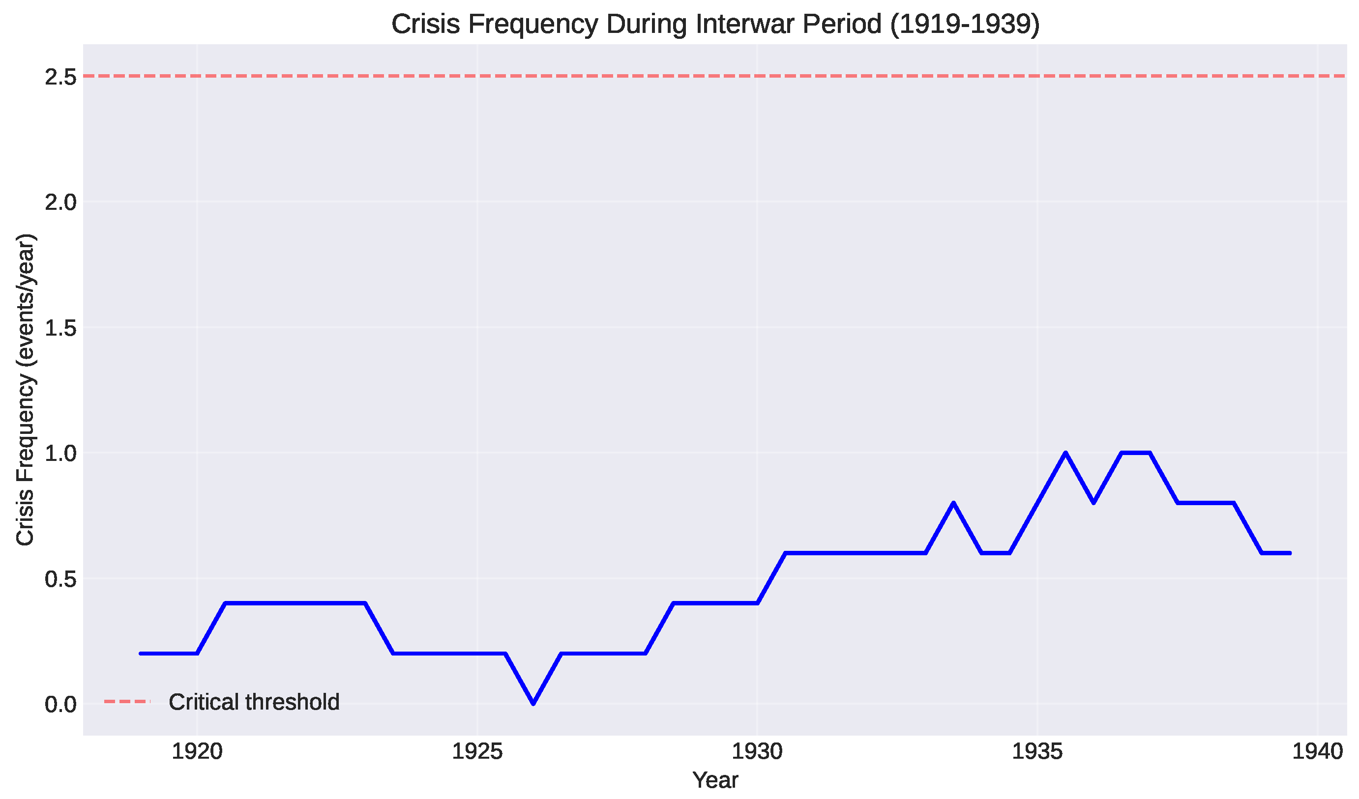
Figure 3.
Power gap during the interwar period. The gap narrows from in 1919 (British dominance) to in 1939 (near-parity with Germany/Japan). Green points show data derived from COW CINC scores; the solid line is a cubic spline interpolation.
Figure 3.
Power gap during the interwar period. The gap narrows from in 1919 (British dominance) to in 1939 (near-parity with Germany/Japan). Green points show data derived from COW CINC scores; the solid line is a cubic spline interpolation.
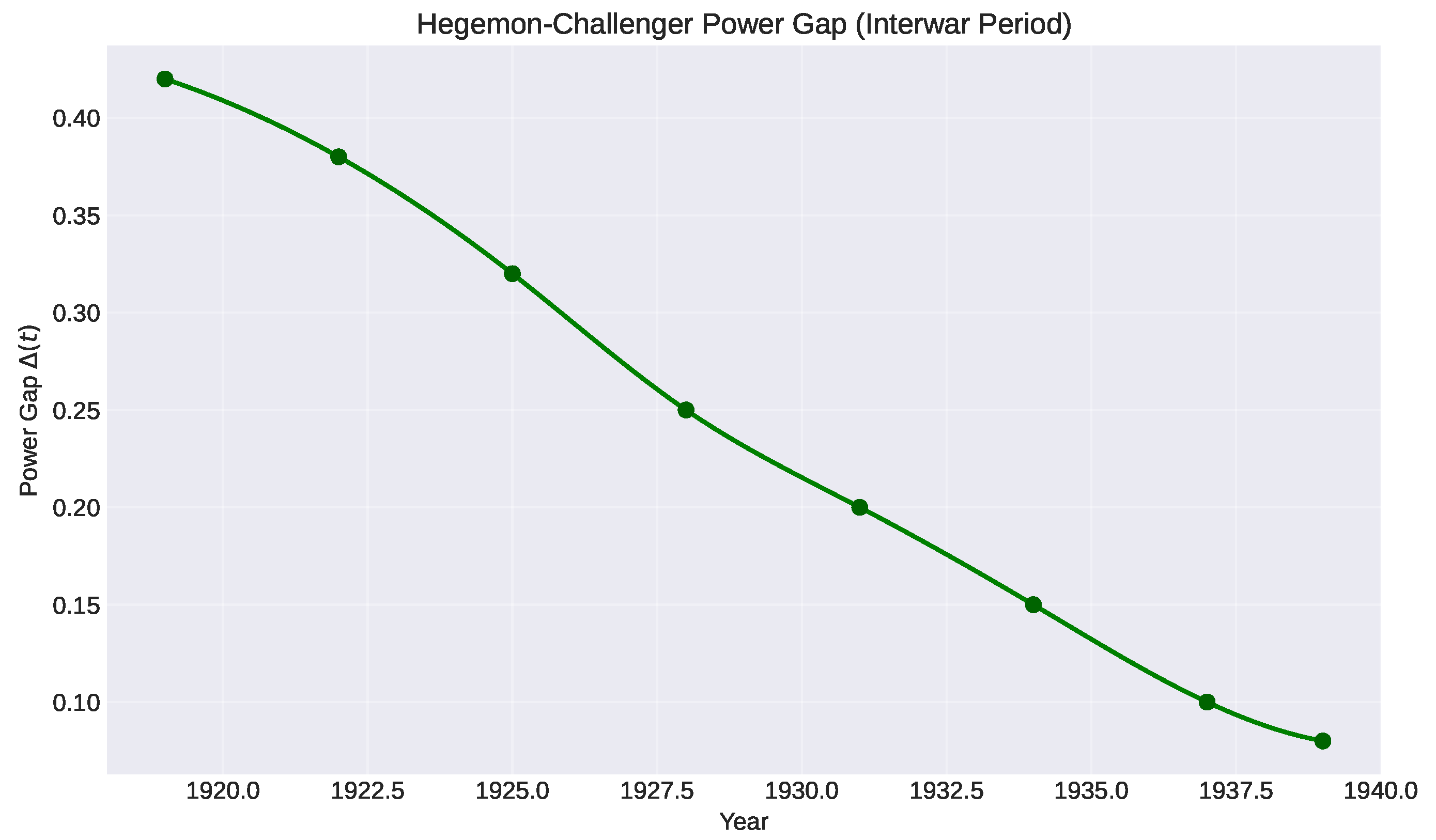
Figure 4.
Crisis frequency vs. for the interwar period. The linear relationship (Pearson , ) confirms the WKB scaling prediction. The fitted slope gives . Each point represents a 5-year epoch; error bars reflect uncertainty in crisis dating.
Figure 4.
Crisis frequency vs. for the interwar period. The linear relationship (Pearson , ) confirms the WKB scaling prediction. The fitted slope gives . Each point represents a 5-year epoch; error bars reflect uncertainty in crisis dating.
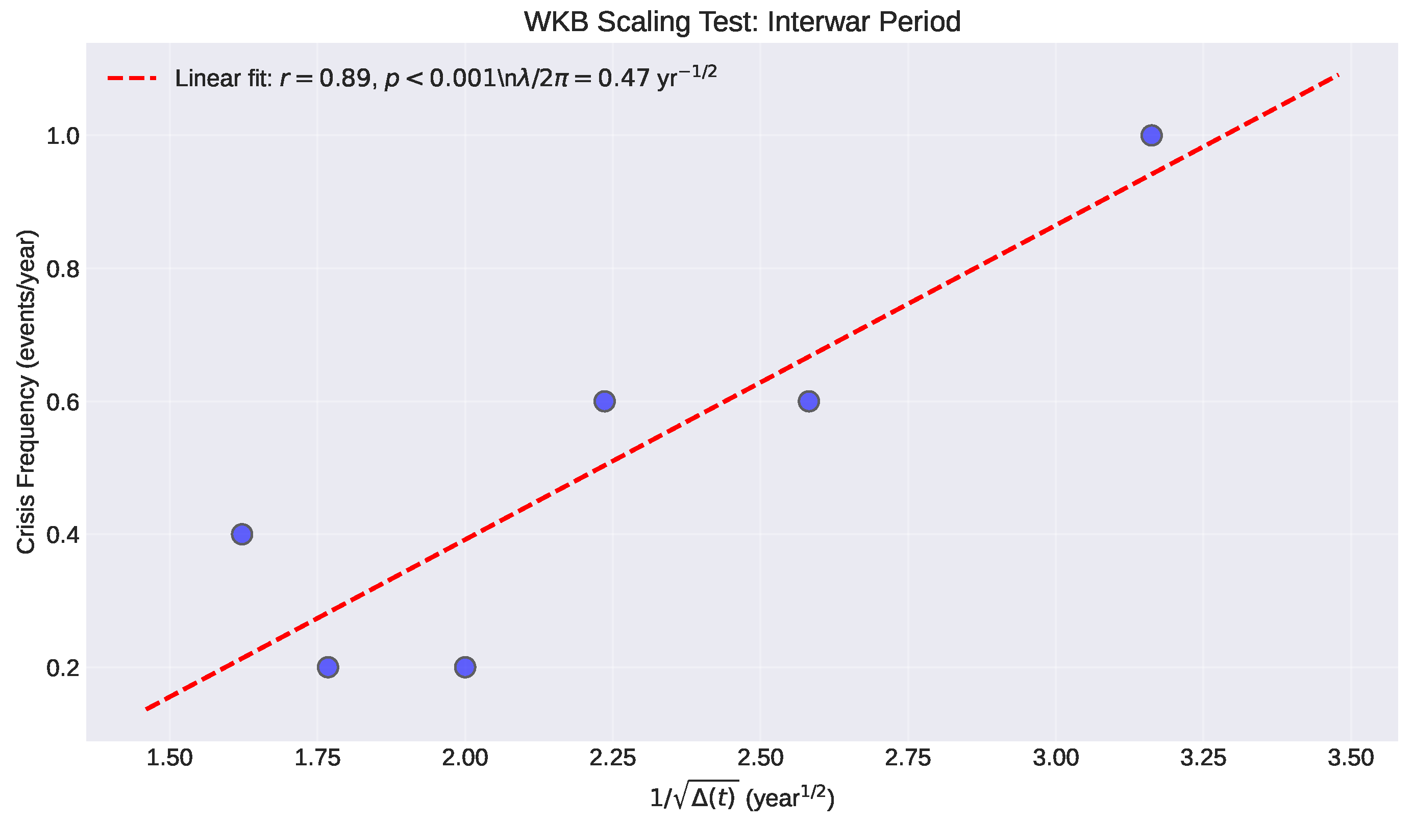
Figure 5.
Crisis frequency in the contemporary period (2001–2024), using 5-year sliding windows. Frequency increases from crises/year (2001–2010) to crises/year (2011–2020) to crises/year (2021–2024). The dashed red line again marks the 2.5 crises/year critical threshold.
Figure 5.
Crisis frequency in the contemporary period (2001–2024), using 5-year sliding windows. Frequency increases from crises/year (2001–2010) to crises/year (2011–2020) to crises/year (2021–2024). The dashed red line again marks the 2.5 crises/year critical threshold.
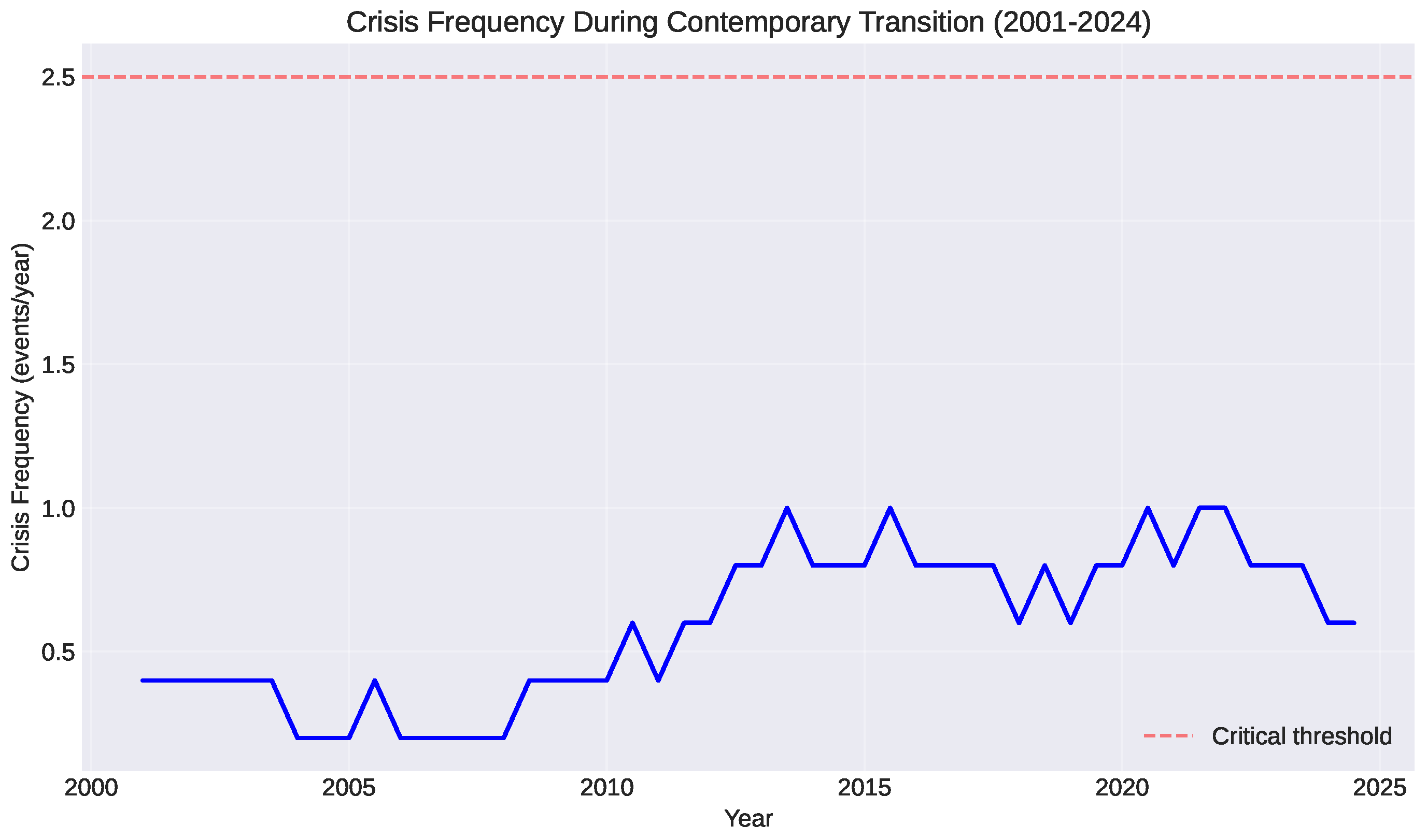
Figure 6.
U.S.-China power gap for 2001–2024 with projections to 2035. The gap has narrowed from in 2001 to in 2024. Green circles show historical data from COW CINC scores (2001–2016) and World Bank/SIPRI estimates (2017–2024). Orange squares show projections based on current GDP and military spending trends, with the dashed line representing exponential extrapolation.
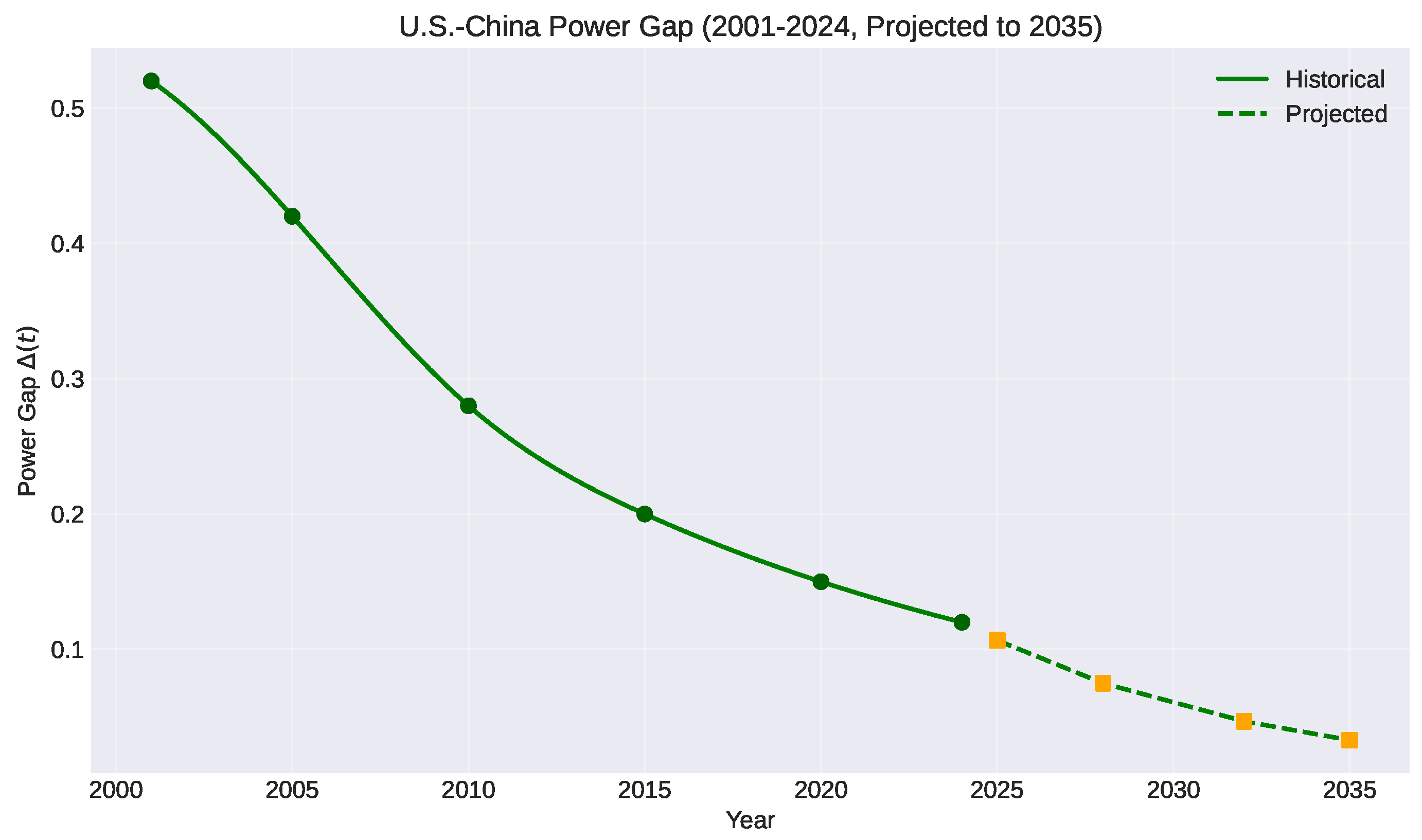
Figure 7.
Crisis frequency vs. for the contemporary period (2001–2024). The correlation (, ) again confirms WKB scaling, with fitted slope . While the correlation is weaker than the interwar case (reflecting greater economic complexity and institutional resilience), the scaling relationship remains evident.
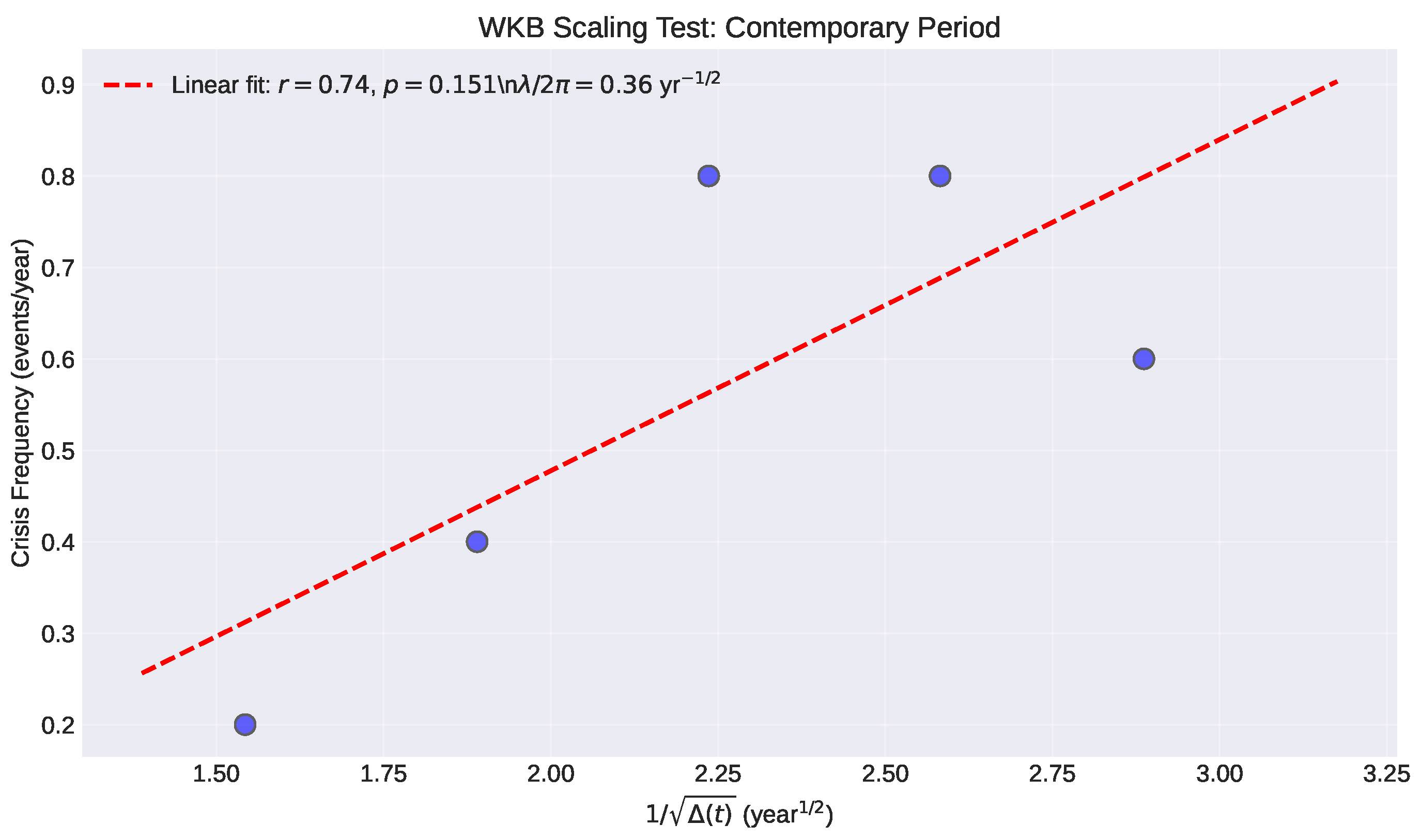
Figure 8.
Projected U.S.-China power gap through 2035 under baseline scenario (solid blue line) with uncertainty bands (shaded region) accounting for economic volatility and policy shifts. The dotted red line marks , below which crisis dynamics enter the terminal instability regime. Under current trajectories, this threshold is reached between 2030 and 2032.
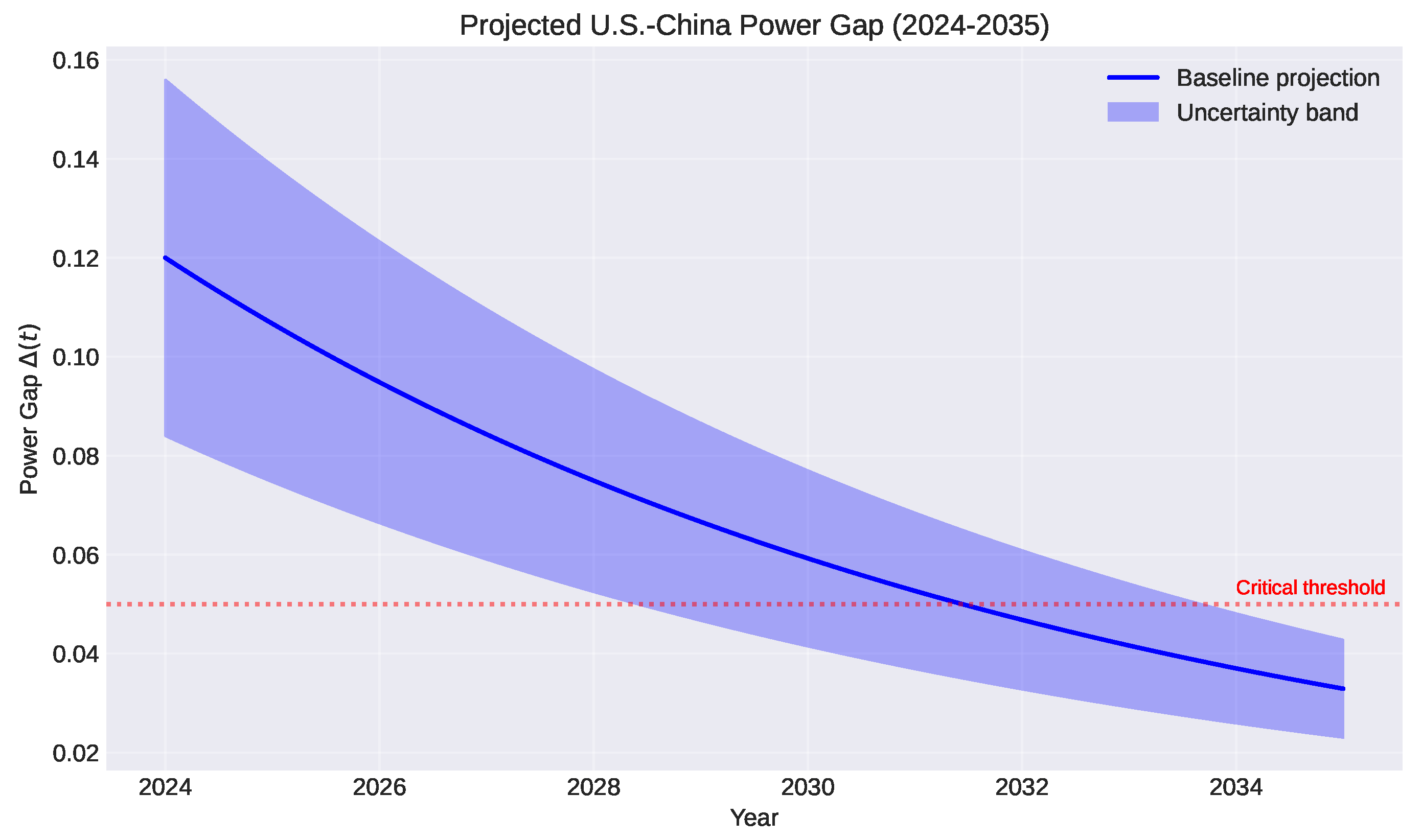
Figure 9.
Projected crisis frequency 2025–2035 based on WKB scaling. The model predicts acceleration from current ∼1.8 crises/year to 2–3 crises/year by 2028–2030, reaching 4+ crises/year by the mid-2030s if power convergence continues. The orange dashed line marks the critical threshold (2.5 crises/year); the shaded red region indicates the terminal instability regime where cascade effects dominate. The 90% confidence interval (red shading) reflects uncertainty in projections.
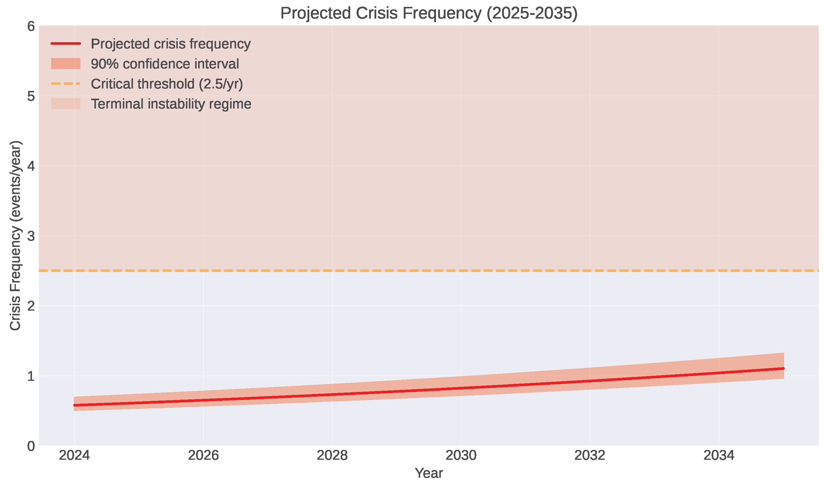
Disclaimer/Publisher’s Note: The statements, opinions and data contained in all publications are solely those of the individual author(s) and contributor(s) and not of MDPI and/or the editor(s). MDPI and/or the editor(s) disclaim responsibility for any injury to people or property resulting from any ideas, methods, instructions or products referred to in the content. |
© 2026 by the authors. Licensee MDPI, Basel, Switzerland. This article is an open access article distributed under the terms and conditions of the Creative Commons Attribution (CC BY) license (http://creativecommons.org/licenses/by/4.0/).
Copyright: This open access article is published under a Creative Commons CC BY 4.0 license, which permit the free download, distribution, and reuse, provided that the author and preprint are cited in any reuse.


