
Submitted:
04 January 2026
Posted:
06 January 2026
You are already at the latest version
Abstract
The Earth flyby anomaly—a small, unexplained residual in spacecraft velocity—remains a persistent challenge in astrodynamics. While the empirical Anderson relation captures the general trend of reported anomalies, it does not account for the suppressed or near-null results observed in several later flybys. Here we construct a geometry-aware, Earth-fixed coupling proxy based on distance-weighted surface visibility over a land-sea distribution mask. We identify a robust sign structure across the primary flyby set that remains stable under variations in weighting choice and integration window. The results indicate that Earth-fixed asymmetry acts as a modulation of the Anderson prediction rather than as an independent force, offering a potential pathway for reconciling discrepancies in anomaly magnitude.
Keywords:
earth flyby anomaly
; spacecraft dynamics
; earth-fixed reference frames
; trajectory geometry
; space geodesy
1. Introduction
1.1. The Flyby Anomaly
The Earth flyby anomaly is a small, unexplained residual in the Earth-centered inertial asymptotic velocity () observed during the hyperbolic encounters of several spacecraft with Earth. First reported following the Galileo 1990 encounter [1], these anomalies typically manifest at the mm/s scale. Despite decades of scrutiny, conventional physical effects—including atmospheric drag, solar radiation pressure, Earth’s albedo, relativistic corrections, and known tracking systematics—have been found insufficient to account for the observed magnitudes [2].
1.2. The Anderson Relation
In their seminal 2008 analysis, Anderson et al. [3] proposed that the change in asymptotic velocity is not a random residual but follows a specific geometric orientation relative to the Earth’s rotation. They proposed a phenomenological relation relating to the spacecraft’s incoming and outgoing velocity declination ():
where is the Earth’s angular rotational velocity; is Earth’s characteristic radius; and c is the speed of light.
While this relation demonstrated high empirical success for early flybys such as NEAR and Galileo I, it does not account for the near-null results of the Juno and Rosetta 2009 encounters.
1.3. Motivation and Scope
While most existing analyses of the flyby anomaly focus on inertial-frame parameters, the rotating and spatially structured nature of Earth motivates consideration of Earth-fixed asymmetries. Previous investigations of tesseral harmonics explored such links between Earth-fixed mass distribution and the anomaly, although reported estimates suggested that these effects are unlikely to constitute the sole driver [4].
Motivated by this distinction, the present work investigates whether a simple Earth-fixed geographic field—specifically a land–sea surface mask—produces a reproducible, trajectory-dependent modulation when averaged over the spacecraft viewing geometry. By mapping flyby trajectories across a view-averaged land-fraction field, we test whether this proxy exhibits consistent sign structure across the primary flyby set.
This study does not claim to explain the flyby anomaly. Rather, it demonstrates that the resulting Earth-fixed proxy yields a robust sign asymmetry that aligns systematically with deviations from the Anderson declination relation. The emphasis is on identifying consistent structure suggestive of a common Earth-fixed modulation, rather than on proposing a physical mechanism.
2. Methods
2.1. Trajectory Data Reconstruction
Spacecraft ephemerides were reconstructed using the NASA NAIF SPICE toolkit, implemented via the SpiceyPy Python wrapper. Essential kernels were retrieved directly from the NAIF PDS directories. SPK kernels were selected to ensure coverage of the flyby encounters.
To ensure high-resolution capture of the interaction window, trajectory data were sampled at 10-second intervals (s). The analysis window was defined radially: data were extracted for all epochs where the spacecraft geocentric distance km.
The spacecraft position vectors were extracted in the International Terrestrial Reference Frame (ITRF93), ensuring that the derived longitude () and latitude () correspond to the rotating Earth surface rather than a non-rotating, inertial celestial reference frame.
2.2. Land-Sea Mask Generation
The Earth-fixed environmental proxy relies on a binary land–sea classification of the Earth’s surface. We utilized the Natural Earth 1:110m physical vector dataset (ne_110m_land) as the source for landmass geometry.
This vector data was saved as a discrete grid with a spatial resolution of (Figure 1). For each grid cell centered at , the binary mask value is given as:
This grid resolution captures major continental-scale structure while maintaining computational efficiency for subsequent path-integration steps.
2.3. Visible Surface Sampling
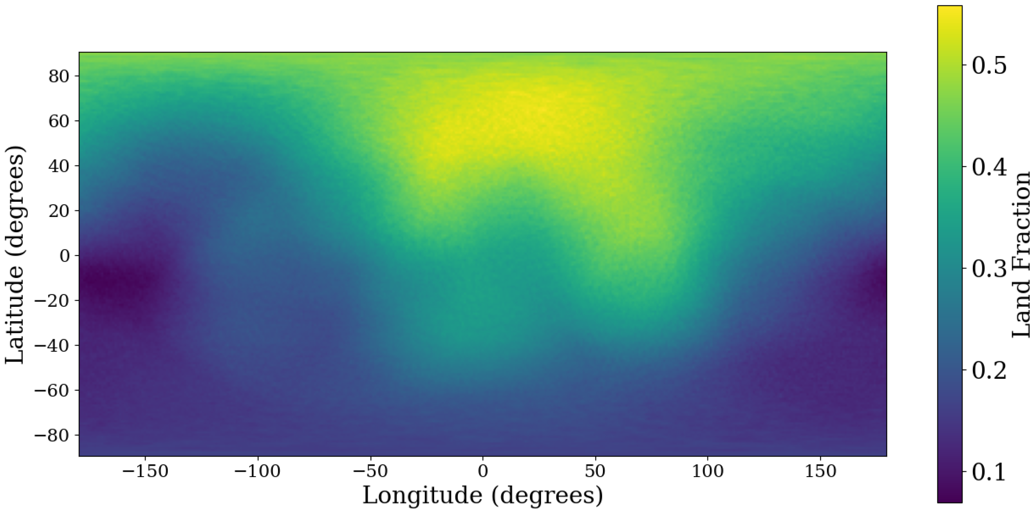
To compute the instantaneous land fraction visible from the spacecraft, we employed a deterministic sampling scheme based on a Fibonacci lattice (golden-spiral) distribution. For a spacecraft at geocentric distance r, the visible Earth surface is defined as the spherical cap bounded by the horizon half-angle (measured from nadir), where . We generated sample points distributed spirally over this cap area. For each visible surface point in the local spacecraft frame, we performed a basis transformation to the earth fixed-frame to determine an array of geodetic coordinates . The instantaneous land fraction is computed as:
where is the binary land value from the land-sea mask. Figure 2 illustrates how view-angle averaging of the binary land mask yields a continuous effective land-weighting field.
Figure 1.
Binary land mask.
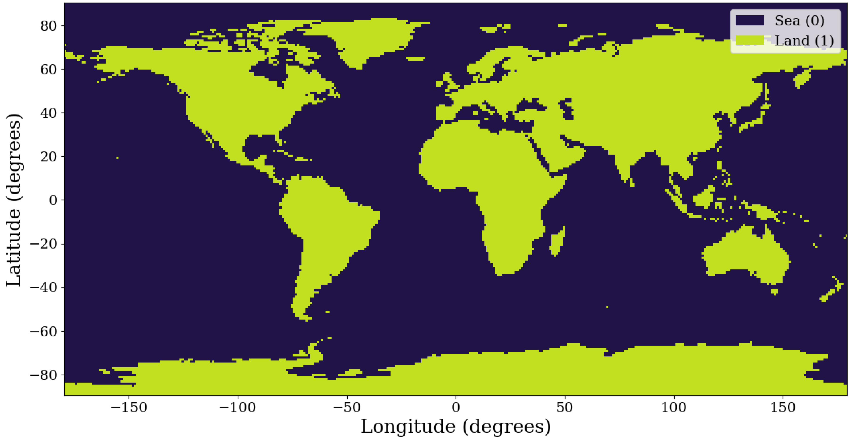
Figure 2.
View-averaged land-weighting field calculated at km
2.4. Coupling Metric Definition
The cumulative Earth-fixed coupling C is defined as the normalized asymmetry between inbound and outbound interaction integrals. The interaction strength is modeled using a distance-dependent weighting function . Motivated by the expectation that surface-mediated contributions decay with altitude, and guided by convergence tests, we adopt an inverse-square geocentric distance weighting:
The total weighted land signal I for a trajectory leg is obtained by integrating over time:
The final coupling proxy C is defined as the asymmetry ratio:
This normalization isolates the geometric contrast of the flyby from effects related to total interaction time or absolute proximity.
2.5. Stability and Robustness Protocols
To ensure the observed asymmetries are not artifacts of arbitrary parameter choices, we implemented two specific robustness tests:
1. Integration Convergence (Plateau Test): We analyzed the stability of C as a function of the integration boundary . The integration window was expanded stepwise from km to km from Earth center to identify the region where the metric stabilizes.
2. Longitudinal Sensitivity (Window Test): To distinguish true geographic correlation from random projection noise, we performed a sliding window test. The entire flyby set coordinates were rotated longitudinally () in 36 discrete increments of . For each rotation, the coupling signs of the entire flyby set were re-evaluated. The stable window was recorded as the continuous fraction of these rotated orientations that reproduce the sign structure observed in the true flyby geometry. Assuming a fixed surface distribution, this procedure is equivalent to introducing a corresponding azimuthal rotation of the land mask.
3. Results
3.1. Trajectory Asymmetry Visualized
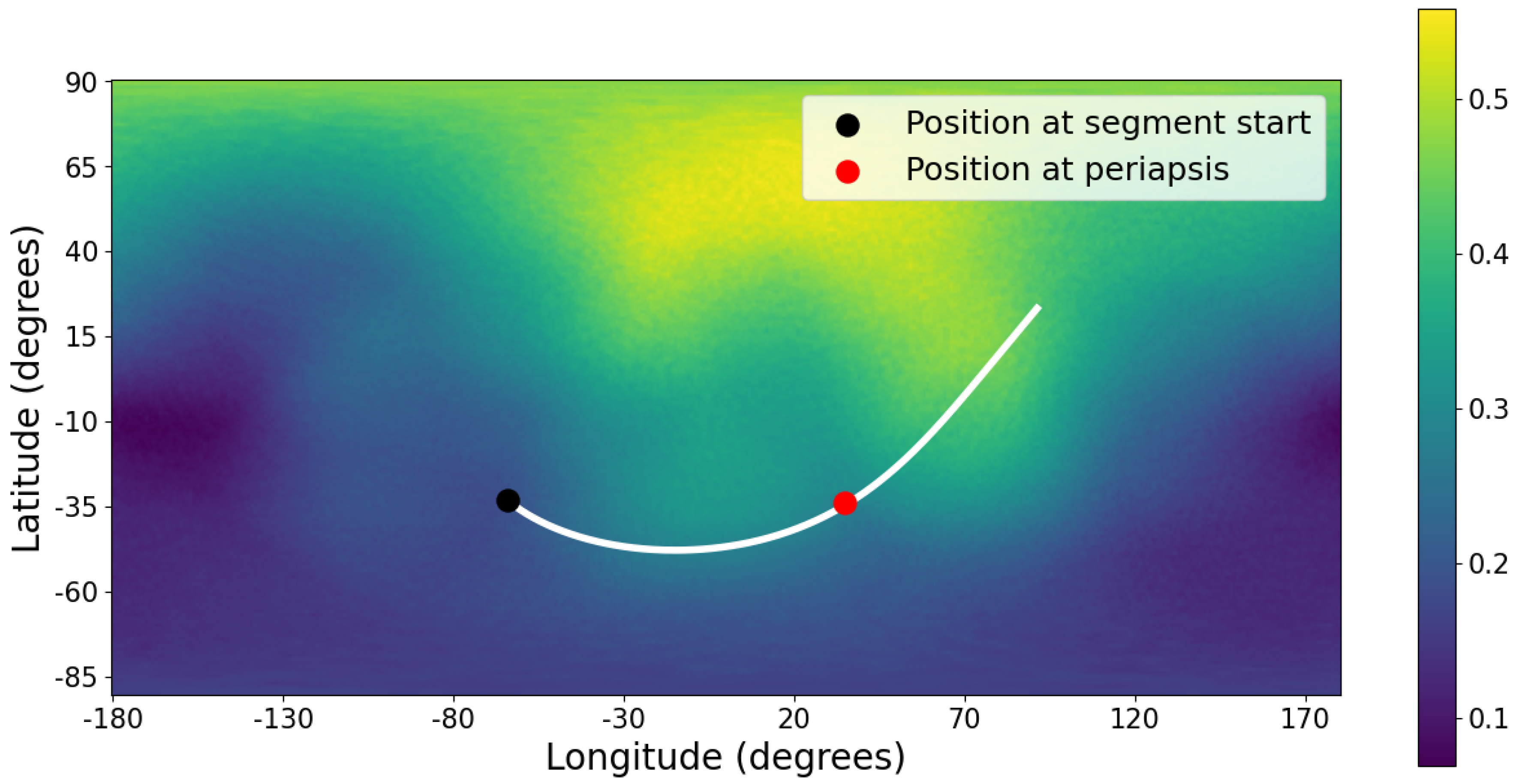
Figure 3 and Figure 4 provide qualitative visualizations of trajectory asymmetry with respect to the view-averaged land-fraction field. Figure 3 shows the Galileo I flyby as a representative example of positive coupling (). Figure 4 shows the Juno flyby as a representative negative-coupling case (). These plots are intended solely to illustrate the geometric origin of the asymmetry and do not represent the precise, distance-weighted surface interaction experienced by the spacecraft.
Figure 3.
Galileo I periapsis-centered trajectory segment over the view-averaged land-weighting field ( km).
Figure 3.
Galileo I periapsis-centered trajectory segment over the view-averaged land-weighting field ( km).
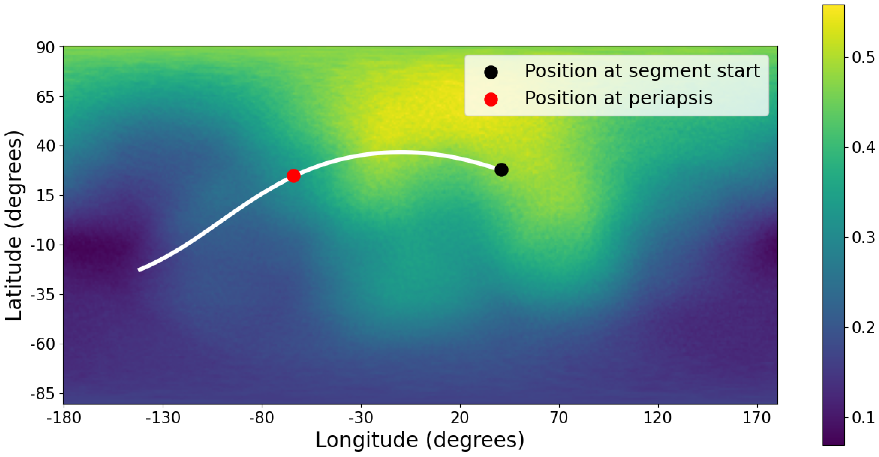
Figure 4.
Juno periapsis-centered trajectory segment over the view-averaged land-weighting field ( km).
Figure 4.
Juno periapsis-centered trajectory segment over the view-averaged land-weighting field ( km).
3.2. Convergence and Integration Domain
To determine the effective range of the Earth-fixed interaction, we examined the accumulation of the coupling proxy C as a function of the integration boundary , spanning km to km.
For the weighting (Figure 5), a clear saturation behavior is observed: the coupling signal approaches a stable plateau at approximately km (chosen post hoc from convergence). Beyond this distance, incremental contributions from the land fraction become minor. To quantify this stability, we compute the percentage drift in the coupling factor (Table 1) when extending the boundary from the plateau point ( km) to the edge of the chosen data window ( km).
In contrast, the weighting and the unweighted case do not exhibit a comparable saturation regime over the same distance range and are not examined further. These alternatives nevertheless preserve the same overall sign structure, noting that the unweighted case begins to diverge in the vicinity of km. Although higher-power weightings (e.g., ) also produce saturation, they impose near-field dominance without clear physical motivation and reduce interpretability. We therefore adopt the lowest exponent that yields a stable far-field regime, namely .
Figure 5.
Long-distance saturation behavior of the coupling proxy under weighting.
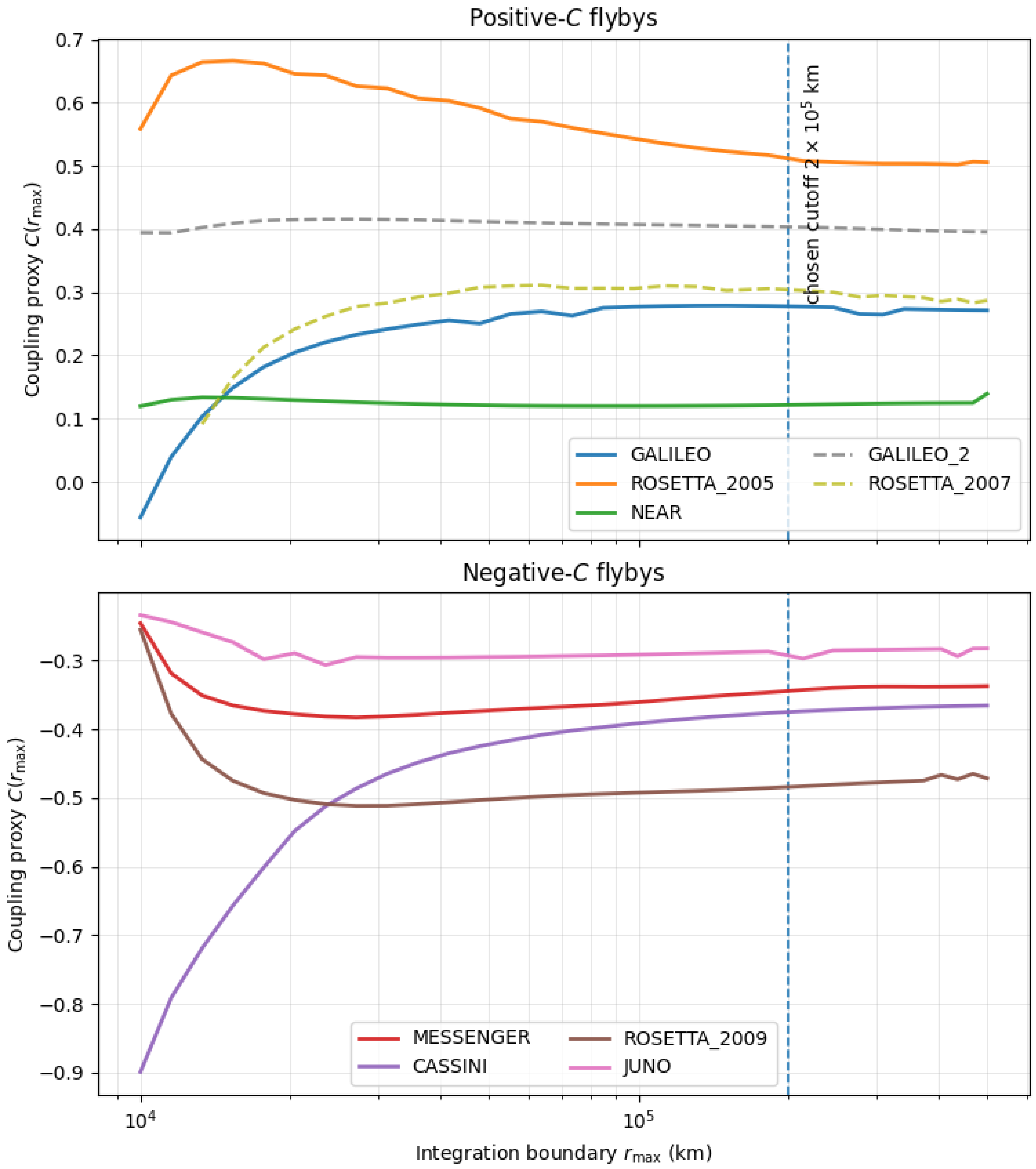
The low average absolute drift () for the weighting confirms that the integration is well-behaved and that the cutoff of km captures the dominant geometric contribution.
3.3. Coupling Factors vs. Anderson Prediction
Adopting km as the standard integration limit, we computed the normalized Earth-fixed coupling C for the primary flyby set spanning encounters from 1990 to 2013. Table 2 compares these values with both the empirical Anderson prediction and the reported velocity anomalies.
A key result is the sign divergence observed for the Juno and Rosetta 2009 flybys. In both cases, the Anderson relation predicts a positive anomaly, whereas the Earth-fixed proxy yields a negative coupling. This negative modulation is consistent with the near-null or reduced anomalies reported for these encounters.
3.4. Longitudinal Stability Test
To probe sensitivity to Earth-fixed longitudinal phase and assess whether the observed sign alignment could arise as a projection artifact, we applied a constant offset to the Earth-fixed azimuth of each trajectory. This procedure is equivalent to rotating the land-sea field by while leaving the flyby geometry and radial history unchanged. The trajectories were rotated in 36 discrete increments (), and we recorded the number of configurations that reproduced the observed sign sequence of the primary flyby set for weighting.
The results of this sliding window analysis are as follows:
- Flybys: Galileo I, Rosetta (2005), NEAR, MESSENGER, Cassini, Rosetta (2009), Juno, Galileo II, Rosetta (2007)
- True Sign Sequence: [ + + + - - - - + +]
- Matching Longitudinal Shift Indices: [0, 1, 2, 3, 4, 5, 6, 34, 35]
- Total Matching Windows: 9 / 36
- Global Match Rate: 0.25
The presence of a limited and contiguous set of matching indices, centered on the true Earth geometry, indicates that the correlation is sensitive to the specific longitudinal configuration of continental structure rather than being a generic outcome of the projection or sampling procedure.
4. Discussion
4.1. Earth-Fixed Modulation of the Anderson Relation
Across the primary flyby set, the Earth-fixed coupling proxy C exhibits a consistent relationship with deviations from the Anderson prediction. When both the observed anomaly and C are positive (Galileo I, Rosetta 2005, Rosetta 2007, and NEAR), the deviation between the measured anomaly and the Anderson estimate is small. The null residual reported for Rosetta 2007 is consistent with its already small Anderson-predicted anomaly.
In contrast, in flybys for which the Anderson relation predicts a positive anomaly but the coupling proxy is negative, Juno and Rosetta 2009 exhibit strong suppression, yielding null observed anomalies; while MESSENGER shows a small reduction relative to the Anderson-predicted magnitude. Cassini represents a particularly informative case: it is the only encounter for which both the Anderson prediction and the coupling proxy are negative, and the observed anomaly is correspondingly shifted further in the negative direction. Excluding the drag-contaminated Galileo II flyby, the only configuration not sampled by the existing dataset is a strongly positive coupling coincident with a negative Anderson prediction. This pattern suggests that the Earth-fixed coupling acts as a modulation of the Anderson relation rather than as an independent contributor.
For flybys with predicted anomaly magnitudes close to or below current detection thresholds (such as MESSENGER and Rosetta 2007), claims of quantitative suppression should be handled cautiously. In such cases, the relevance of the coupling proxy lies primarily in directional modulation rather than in quantitative magnitude reduction.
The proposed interpretation is falsifiable. The pattern would be broken if, for a positive Anderson prediction, a strongly negative coupling were observed without suppression or if a positive coupling within the observed range produced strong suppression.
4.2. Structural Coherence Versus Mass Distribution
If the observed correlation reflects a genuine physical effect, it is unlikely that the land-sea mask is acting primarily as a proxy for surface mass differences. The land-sea classification used here is binary and minimally structured, and does not encode information about crustal density, detailed topography, or gravitational harmonics. Instead, the coupling proxy appears to emphasize differences in spatial organization or large-scale structural coherence tied to Earth-fixed geography.
While certain astrophysical systems exhibit a decoupling between gravitational signatures and visible baryonic structure—most notably the Bullet Cluster—no established framework directly links structural organization itself to gravitational behavior. Nevertheless, such observations illustrate that gravitational influence need not always align straightforwardly with visible mass distributions. In this context, it remains possible that future extensions of gravitational or dynamical modeling that explicitly encode spatial organization, anisotropy, or environment-dependent coupling—rather than treating mass distributions solely as scalar sources—may be required to fully account for the behavior observed here.
4.3. Convergence, Weighting, and Sign Stability
Distance weighting is introduced in the coupling proxy to ensure convergence of the interaction integral. However, the persistence of coupling sign across multiple weighting choices and integration windows indicates that the weighting scheme does not fundamentally determine the direction of the effect. Instead, weighting primarily governs the spatial scale over which the proxy stabilizes.
The observation that flyby anomalies manifest as constant offsets after encounter completion is consistent with an interaction or modulation that decays rapidly with distance from Earth. This behavior supports an interpretation in which the effect is driven by the near-Earth environment rather than by long-range perturbations accumulated over extended orbital arcs.
4.4. Limitations and Outlook
This study is exploratory and rests on a phenomenological correlation observed across a limited dataset. While the sign structure of the coupling proxy is robust to variations in windowing, weighting, and longitudinal phase, the number of available Earth flybys constrains statistical generalization. Additional Earth encounters are unlikely to provide sufficient new data to resolve the effect conclusively. Nevertheless, similar analyses applied to other planetary flybys or spacecraft interactions involving rotating, structured bodies may offer opportunities to test whether the modulation behavior observed here is specific to Earth or reflects a more general feature of flyby dynamics.
4.5. Code Availability
All analysis code used to generate the results presented in this work is publicly available at https://github.com/yfikret/earth-fixed-flyby-modulation. The repository includes scripts for trajectory reconstruction using SPICE, land-sea mask generation, surface visibility sampling, and coupling metric evaluation.
The code is provided to support transparency and reproducibility of the analysis. While the implementation reflects the methodology described here, users are encouraged to independently verify results and assess sensitivity to alternative modeling choices.
Acknowledgments
The author acknowledges the use of automated tools for drafting assistance and discussions that helped clarify the structure and presentation of this work. Any remaining errors or omissions are solely the author’s responsibility.
References
- Antreasian, Peter; Guinn, Joseph. Investigations into the unexpected delta-v increases during the earth gravity assists of galileo and near. AIAA/AAS Astrodynamics Specialist Conference and Exhibit, 1998; p. 4287. [Google Scholar]
- Lammerzahl, Claus; Preuss, Oliver; Dittus, Hansjorg. Is the physics within the solar system really understood? In Lasers, Clocks and Drag-Free Control: Exploration of Relativistic Gravity in Space; Springer, 2008; pp. pages 75–101. [Google Scholar]
- Anderson, John D; Campbell, James K; Ekelund, John E; Ellis, Jordan; Jordan, James F. Anomalous orbital-energy changes observed during spacecraft flybys of earth. Physical Review Letters 2008, 100(9), 091102. [Google Scholar] [CrossRef] [PubMed]
- Acedo, L. On the effect of ocean tides and tesseral harmonics on spacecraft flybys of the earth. Monthly Notices of the Royal Astronomical Society 2016, 463(2), 2119–2124. [Google Scholar] [CrossRef]
- Acedo, L. The flyby anomaly: a multivariate analysis approach. Astrophysics and Space Science 2017, 362(2), 42. [Google Scholar] [CrossRef]

Table 1.
Percentage drift of coupling factor C between km and km.
| Flyby | (%) | (%) | Unweighted (%) |
|---|---|---|---|
| NEAR | 14.7 | 46.5 | 71.8 |
| Galileo I | -2.27 | -27.0 | -87.6 |
| Galileo II | -2.00 | -27.1 | -86.8 |
| Rosetta (2005) | -1.74 | -10.5 | 55.3 |
| Rosetta (2007) | -5.63 | -43.5 | -126 |
| Rosetta (2009) | -2.60 | -28.4 | -92.9 |
| Juno | -1.41 | -15.1 | -35.9 |
| MESSENGER | -2.03 | -20.0 | -198 |
| Cassini | -2.49 | -20.3 | -56.5 |
| Average absolute drift | 3.87 | 26.5 | 90.1 |
Table 2.
Comparison of Earth-Fixed Coupling (C), Anderson predictions, and observed anomalies
| Flyby | Observed (mm/s) | Anderson (mm/s) | C (Sign) | C (Value) |
|---|---|---|---|---|
| NEAR [3] | 13.46 | 13.28 | (+) | 0.122 |
| Galileo I [3] | 3.92 | 4.12 | (+) | 0.278 |
| Galileo II [3] | -4.6 | -4.67 | (+) | 0.403 |
| Rosetta (2005) [3] | 1.80 | 2.07 | (+) | 0.514 |
| Rosetta (2007) [5] | 0 | 0.523 | (+) | 0.304 |
| Rosetta (2009) [5] | 0 | 1.10 | (-) | -0.484 |
| Juno [5] | 0 | 6.34 | (-) | -0.286 |
| MESSENGER [3] | 0.02 | 0.06 | (-) | -0.344 |
| Cassini [3] | -2 | -1.07 | (-) | -0.375 |
Disclaimer/Publisher’s Note: The statements, opinions and data contained in all publications are solely those of the individual author(s) and contributor(s) and not of MDPI and/or the editor(s). MDPI and/or the editor(s) disclaim responsibility for any injury to people or property resulting from any ideas, methods, instructions or products referred to in the content. |
© 2026 by the authors. Licensee MDPI, Basel, Switzerland. This article is an open access article distributed under the terms and conditions of the Creative Commons Attribution (CC BY) license (http://creativecommons.org/licenses/by/4.0/).
Copyright: This open access article is published under a Creative Commons CC BY 4.0 license, which permit the free download, distribution, and reuse, provided that the author and preprint are cited in any reuse.


