
Submitted:
14 November 2024
Posted:
18 November 2024
You are already at the latest version
Abstract
Extraterrestrial impacts, ranging from minor asteroids to larger bodies, induce varying degrees of atmospheric perturbation, with potential consequences ranging from localized disruptions to global events. This study investigates the ionospheric disturbances caused by a meteoroid impact over the Caribbean Sea on June 22, 2019. Detected by U.S. government sensors and the Geostationary Lightning Mapper (GLM), the event released approximately 6 kilotons of energy, marking the most energetic meteoroid impact recorded by both databases. We used data from the UNAVCO network of GNSS stations, alongside energy estimates derived from GLM light curves and USG sensors, to identify significant variations in Total Electron Content (TEC) associated with the meteoroid's atmospheric passage. Advanced detrending techniques, including the Savitzky-Golay filter, were employed to enhance wave-like features within the TEC time series, confirming their correlation with the meteoroid event. Additionally, the analysis confirms minimal solar activity during the event, ruling out solar terminator effects as a major contributor to the observed disturbances. This study underscores the need for continued research into ionospheric perturbations from meteoroid impacts, with future work focusing on modeling TID propagation velocity and refining detection techniques using tools such as the Rate of TEC Index (ROTI).
Keywords:
Meteoroids
; Atmosphere
; Ionosphere
; Plasma Physics
; TEC
1. Introduction
Bolides impact the Earth daily, ranging from small objects ( m) that disintegrate upon atmospheric entry to larger ( m), rare events capable of causing global disturbances. If their diameter is greater than 1 km the impact can be considered a global catastrophe [1,2]. Some famous modern cases are the Tunguska event 1n 1908 [3] and the Chelyabinsk event [4] in 2013.
In addition, the General Civil Protection Law in Mexico, amended in June 2014, incorporated near-Earth objects (NEOs) into the list of natural hazards phenomena [5]. The legislation mandates that the National Center for Disaster Prevention (CENAPRED) establishes responsibilities and the Mexican Space Agency to establish national action protocols in case of meteorites. Meteorite impacts and NEOS are also included in the UNDRR "Hazard Definition and Classification Review" [6], denoting their importance for the international community.
As bolides passes through the Earth’s atmosphere at hypersonic velocities, and posterior breakup, may produces turbulence, wave processes, etc. Thus leading to displacements of air, which produces Acoustic Gravity Waves (AGWs). AGWs can reach ionospheric levels and be detected as Traveling Ionospheric Disturbances (TIDs). Such events have been recently recorded in certain databases, such as the Center for Near Earth Objects Studies (CNEOS), Jet Propulsion Laboratory (JPL) and the Geostationary Lightning Mapper (GLM) publicly available at https://cneos.jpl.nasa.gov/fireballs/ and https://neo-bolide.ndc.nasa.gov/#/, respectively.
We picked our interest in one certain event, that we nicknamed “the Caribbean Meteoroid.” This meteoroid is the most energetic which appears in both databases and thus is an interesting case for studying the potential TID that could be produced. To do so, we collected Receiver INdependent EXchange (RINEX) data from nearby GNSS stations from the UNAVCO network (also publicly available 1) and developed a method to detrend the resultant TEC series and estimate the TIDs propagation speed.
The Figure 1 depicts a bright flash of light generated by the impact of a small Near-Earth Object (NEO) upon entering Earth’s atmosphere on June 22, 2019, over the Caribbean region. The flash, captured in a sequence of images, highlights the precise moment of the meteoroid’s entry and its interaction with the upper atmosphere just prior to disintegration. The image reveals a radiant expansion of energy, corresponding to the heat and pressure release caused by the meteoroid as it traverses the upper layers of the atmosphere. This visual context is critical for understanding the ionospheric disturbances induced by this event, which are discussed throughout the study.
Our approach involved advanced signal processing techniques, such as the Savitzky-Golay filter [7], to enhance the signal quality of the TEC time series. This allowed us to isolate wave-like features indicative of TIDs. We analyzed the spatial and temporal patterns of the disturbances to ascertain their velocities and directions of propagation, which are crucial for understanding the dynamics of ionospheric responses to meteoroid impacts [8].
Furthermore, we correlated these disturbances with the estimated impact energy derived from GLM light curves to establish a relationship between the meteoroid’s energy and the magnitude of ionospheric disturbances observed Maruyama et al. [9]. By comparing our findings with background ionospheric conditions, we aimed to delineate the influence of this specific meteoroid event against natural variability [10].
Our study not only sheds light on the immediate effects of meteoroid impacts on the ionosphere but also sets the stage for future investigations into similar phenomena, highlighting the need for more robust methodologies in detecting and analyzing TIDs caused by various atmospheric disturbances [11]. This research contributes to a broader understanding of the role of meteoroids in modifying the ionospheric environment and paves the way for advancements in predictive models for space weather events [12].
2. Data Processing
2.1. Meteor Location and Trajectory
The entry of the Caribbean meteor into the atmosphere was identified and studied its behavior and impact in the ionospheric region. To do so we used data from the GLM [13] and the CNEOS of the JPL of the NASA. We used the interactive database of both projects, available at https://neo-bolide.ndc.nasa.gov/#/ and https://cneos.jpl.nasa.gov/fireballs/. From CNEOS database, we found basic physical parameters such as event coordinates, altitude, total velocity and its components, total radiated energy and calculated impact energy. These data are shown in Table 1. On the other hand, from GLM we got the meteor light curve, accurate position of the fragments and duration event. The use of both databases allowed us to cross-verify the detection data, providing complementary information about the meteor’s properties due to the independent nature of their measurements.
According to the CNEOS database records, the total energy is about 1.4% of the Chelyabinsk bolide, and fragmentation occurred above the open sea, at afternoon or near sunset depending on the closest mainland available: from Dominican republic, Puerto Rico, the lesser Antilles, Venezuela, Guyana, French Guyana and Suriname.
3. RINEX Data
In order to study the ionospheric behavior, we use the RINEX data for event from 38 stations that surrounded the meteor detection coordinates for the day of the event. Since the event occurred near UT midnight, we also obtained GNSS data for the next day in case of there would be TIDs detected several hours after the fragmentation. Using a software developed by Gopi K. Seemala [14], publicly available at https://seemala.blogspot.com/, we computed the slant TEC (sTEC) and vertical TEC (vTEC) for different GNSS satellites, each one identified with a PseudoRandom Noise code (PRN). The behavior of the TEC curve is due to many factors, including the Earth’s rotation, solar activity, etc. TID’s and wave-like curves are not as prominent and are difficult to identify. Due to the sample size, the detrending process necessitates manual intervention to ensure precise data interpretation [15]. In Appendix A1 shows the stations names, coordinates and proper citations.
3.1. Detrending Process
For detrending our data we used a method developed for detecting plasma bubbles in the equatorial region [16], but proved to be effective for detecting AGWs and TIDs. With this method we are able to infer the trend from our TEC data using a Savitzky-Golay filter [16,17]. However, the results of this filtering are sensitive to the parameters we explored or use for such filtering, thus altering significantly the quality of the detrended signal. The TEC time series are assumed to be an additive combination of a signal and a trend [15,18]. Thus we tested the method of Pradipta et al. [16] over the sum of a known signal and a known trend and find the parameters of the Savitzky-Golay filter that recover in the best way the original signal. We used a test signal with the purpose to find out the most appropriate parameters for the filter and we show its functional form in Appendix B.
3.2. Comparison with ARTU data for Chelyabinsk meteor
Our final test was to compare our resulting time series with the results of another, more documented event: the 2013 Chelyabinsk meteor impact. Yang et al. [4] obtained TEC time series by analyzing the coherence spectrum of TEC measurements with many GNSS stations distributed in Russia, United States, and Japan, with the ARTU station being the closest to the meteor impact location. Then, using the most prominent detected frequencies (4.0-7.8 mHz and 1.0-2.5 mHz), they reconstructed the TEC series for PRN 18 and 26. This methodology aligns with previous findings that emphasize the significance of frequency analysis in identifying ionospheric disturbances [19].
Thus, we obtained the RINEX data for the ARTU station and detrended the data using the method described in this paper for the ARTU-PRN18 and ARTU-PRN26 station-satellite links. The results are shown in Figure 2. In this case, we have noticed that the positions of the resulting AGWs align, so we can be confident in our method, which is consistent with the work of [4] with TIDs periods of around 20 min. However, it is also noteworthy that the shape of the detrended time series is not the same due to the fact that it is actually the superposition of all the frequencies involved [20].
Additionally, we already knew where the produced ionospheric perturbation occurred. Finding and distinguishing ionospheric perturbations using this method can be a difficult task, but it has proven to be an accessible confirmation method. This aligns with the conclusions of previous research that highlights the utility of detrending techniques in isolating significant disturbances from background noise [21].
4. Meteor Physical Properties
Using the estimation of the meteor energy and velocity from Table 1, the trajectory angle estimated in Appendix A from the velocity components of and assuming the meteor has a density of 4000 kg m−3, roughly consistent with the composition of chondrites [22], we estimated the initial velocity, initial mass and entry angle of the Caribbean meteor, enlisted in Table 2, by using a system of equations that models the dynamics of a meteoroid passing through Earth’s atmosphere [23]. Solving numerically this set of equations we modeled the Caribbean meteor evolution as passing through Earth’s atmosphere. In Figure 3, Figure 4 and Figure 5, we show the evolution of meteor parameters as it passes through the atmosphere.
In Figure 3, we see that after breakup mass and velocity drops fast to zero, this is due that after breakup these graphs show the mass and velocity of the fragment cloud, which is more susceptible to dissipation, explaining the fast mass drop, each individual fragment into the cloud is easily slowed down by the atmosphere, explaining the velocity drop. The model lost trace of the fragment cloud mass slightly below 30 km. On the other hand, the trajectory angle changes with height linearly in about one degree similar to the suggested by [20,24,25].
The meteor diameter and density are shown in Figure 4, we see for density in left panel that it drops drastically at 40 km approximately due that the density considered after breakup is for the fragmentation cloud, where all the meteor fragments are scattered in a greater volume, for the same reason in the right panel the diameter increases from the same height [26].
Finally, we obtained the meteor energy and pressure, shown in Figure 5. We observe the meteor energy as a function of height, which decreases after breakup and the burst, since most of this energy was released after the burst, which is behavior similar to that suggested by [3,27]. The deposited energy is shown in top panel of Figure 5, where it is discernible a similar behavior however is similar but it has maximum around a height of 40 km. Finally the pressure is shown in right panel, where the meteor stagnation pressure is also displayed. When the meteor pressure exceeds the stagnation pressure it increases dramatically until a maximum at km.
5. Estimated meteor trajectory
Using the data obtained from the model explained in the former section, we estimated the meteor trajectory. The data extracted from the model is shown in Table 3.
With these data, the meteor trajectory can be estimated as follows:
Where L and correspond to the latitude and longitude as a function of height h, respectively, the 0 sub-index correspond to the position where measurements started, in this case km, v is the meteor velocity, is the trajectory angle, is the radius of Earth and is the trajectory angle respect to the equator, assumed to be constant since Coriolis force is negligible for this case, and computed from the components of the meteor velocity in Table 1. Following the results described in §4, we found that a linear relation between time and height, being m the proportionality constant. For heights above 70 km until the Ionospheric Piercing Point (IPP), at 350 km we assumed that the meteor was moving at constant speed equal to the terminal velocity and we supposed a linear relation between trajectory angle between height and trajectory angle .
6. Ionospheric Background and sTEC Time Series
Ionospheric perturbations can take place due to space weather conditions, with an origin from solar events affecting the Earth environment by radiation or charged particles. So, in order to discard such events we investigated the space weather conditions in the day each event occurred. We investigated the solar wind parameters in the event day and the previous 7 days, the x-ray flux and the Dst index at the event date.
6.1. Dst Index
Measurements of the Dst Index were obtained from WDC for Geomagnetism, Kyoto DST index service (https://wdc.kugi.kyoto-u.ac.jp/dstdir/). From these data, we found out that Dst index remains practically constant around zero, which confirms that there were not geomagnetic storms that could prevent us from detecting TIDs in our GNSS data, see Figure 6.
6.2. Solar Wind
The solar wind is part of the space weather events that we should take in account (in order to confirm if TIDs produced by the meteor passage are viable to be detected or no) is unusual solar wind behavior or even coronal mass ejections. To do so, we collected data from the Deep Space Climate Observatory (DSCOVR) of solar wind speed, temperature, density, dynamic pressure and solar magnetic field, in order to monitor the solar wind behavior in the day of the event and the previous 6 or 7 days.
Potential shock waves produced by rapid wind transitions were considered reaching slow wind, which also may produce TIDs and thus contaminating our GNSS data, and may not be distinguishable from TIDs produced by the meteor passage. To check the presence of such shock waves, we estimate the relative velocity of solar wind of one day respect the previous one. The results are shown in Figure 7, where we observe that this velocity is almost constant and gives no chance for a fast stream reaching a slow that could produce a shock wave.
6.3. X-Rays Flux
X rays can be produced in solar flares impacting directly the ionospheric layer. A sudden increase of the flux or sudden variations may be a source of AGW or giving appearance of AGW. We investigated the X ray flux at the event date and the previous week, and collected data from the NOAA Space Prediction Center. A thorough review confirmed the absence of type C, M, or X solar flares capable of impacting Earth’s ionosphere during the period in question.
6.4. Solar Terminator
When a meteoroid enters the atmosphere and experiences subsequent breakup or burst near the solar terminator, the influence of the terminator’s passage on ionospheric conditions warrants careful consideration. Acoustic gravity waves (AGW), observed near the terminator region, are known to induce significant disturbances in the ionosphere [18]. Therefore, disentangling meteoroid-induced effects from terminator-related phenomena in such scenarios requires a comprehensive analysis that accounts for the potential contributions of both sources [28]. Figure 8 shows that meteor burst occurred outside the solar terminator, but some GNSS stations (KOUG and KOUR) are located close to (20 minutes after the fragmentation). In an effort to distinguish between the effects of the meteor and the solar terminator we detrended GNSS data for the mentioned stations at dates prior of the meteor fall, those dates are close enough to guarantee that the sunset occurs at different times. According to the previous, we can isolate the effects of the solar terminator and analyze its effects to check how they could affect time series. Some results are shown in Figure 9 for station KOUG, PRNs 2 and 12. In these cases we see that the solar terminator perturbs the ionosphere, and its effects can bypass the detrending process, since they consist in wave-like variations of TEC. However, these perturbations are typically weak and can be distinguished from those generated by meteor passage, allowing us to confidently conclude that they do not significantly affect our detections. Even more, comparing time series from previous days it can be helpful us to discriminate between time series with detected TID from others where only noise is recorded since some patterns in the time series can be detected. The time series that are similar with the previous days can be classified as non detections.
6.5. sTEC Time Series
We processed the satellite-receiver time series collected from all stations, analyzing each series separately to identify wave-like features through visual inspection. Caution is required when drawing conclusions regarding the presence of TIDs or AGWs associated with the bolide, as ionospheric perturbations induced by the meteor passage may be confounded with other types of ionospheric disturbances. A significant sample of about 10% of all the time series are depicted in Figure 10 and Figure 11.
To facilitate the organization of data and trace spatially the propagation of TIDs, we divided the GNSS stations into 5 sets, roughly based in their location. The spatial distribution of sets and stations is shown in Figure 12.
After analyzing data related to TIDs, the analysis indicates that the stations detecting TIDs are part of sets 3, 4 and 5, which are located southeast of the meteor detection site. It is suspected that TIDs were generated at the position where the meteor crossed through the IPP and propagated away from the source. To estimate such position, we reconstructed the meteor trajectory using the results of the flight equations [24], but these results only were useful up to a height of 70 km. To reconstruct the rest of the trajectory, we observed that before breakup the meteor was moving at a terminal velocity of kms−1, and then extrapolated the linear correlation between trajectory angle and height (see, for example, Figure 3). The resultant trajectory is also shown in Figure 12, as well as the positions of breakup and the meteor crossing the IPP (blue star), from where the TIDs should have been generated (TIDs source from this point). Stations from set 3 and a few from set 4 were close enough to detect TIDs as they passed through. In fact, TIDs were detected for stations located at the south of the meteor estimated trajectory. Set 1 stations were the farthest of the TIDs source. If stations of this set detected anything, the TIDs amplitude after traveling such distances should have been diminished, and become indistinguishable from local noises. The same applies for stations from set 2, but is evident that we did not find TIDs from this set of stations, since the distance to the TIDs source is much shorter, and is also evident that the stations from set 4 and 5 detected TIDs farther from the source. To explain this situation, an independent detection method should be used as corroboration. In this context, we used ROTI index for high resolution data in order to study this.
6.6. High Resolution Data and ROTI Estimation
We employ high resolution GNSS data (1 Hz) from a subset of stations enlisted in Table A1 of Appendix A. From these data, we recalculated dTEC in order to see if the dTEC changes correlated with the meteoroid event. By employing the ROTI method, we were able to quantify the rapid fluctuations in TEC that typically accompany TIDs. ROTI is a useful tool for assessing ionospheric irregularities, as it highlights variations that may not be evident in standard TEC measurements [29].
The dTEC time series were analyzed before, during, and after the impact to capture the temporal evolution of the disturbances. This analysis allowed us to observe significant spikes in dTEC that corresponded with the expected arrival time of the TIDs generated by the meteoroid’s atmospheric entry. The use of high-resolution data enhanced our ability to detect these transient events, providing a clearer picture of their propagation characteristics [30,31].
Furthermore, by applying statistical methods to the ROTI values, thresholds were established to identify significant disturbances linked to meteoroid impacts. This approach not only improves our detection capabilities but also contributes to understanding the broader implications of such events on ionospheric dynamics [31]. Our findings emphasize the importance of using high-resolution GNSS data and advanced analysis techniques to accurately capture the intricate behavior of the ionosphere during meteoroid-induced disturbances.
Nevertheless, with such data, ROTI may be computed. It is defined as the standard deviation of the rate of change of TEC (ROT) within an interval of 1 minute and is computed forward in time through moving average. Low resolution data provides insufficient information to compute satisfactorily the ROTI, but high resolution data solves this issue. In Figure 13, we compare the computed ROTI for station CN40 for satellites with PRN 2, 5, 6, 9, 12 and 15 (which seems to be the most probable TIDs detections) against the detrended data.
Scintillation indices such as S4 and are not available in this study, but ROTI and Multipath (MP) are correlated with scintillation under certain circumstances that are fulfilled in this study [32]. MP is computed with the following the equation:
where N is the number of data points, is the total electron content at time i, and is the mean TEC over the observation period. This approach helps to quantify the fluctuations in TEC that arise from multipath effects, which can occur when satellite signals reflect off nearby surfaces before reaching the receiver.
In our analysis, we focused on periods of high ionospheric activity associated with the meteoroid impact. By correlating MP with ROTI, we aimed to enhance our understanding of how these metrics interact and their implications for ionospheric disturbances. Previous studies have shown that higher multipath effects often coincide with increased scintillation activity, particularly during geomagnetic storms and other significant ionospheric events [33,34].
These insights are crucial for interpreting the overall impact of the meteoroid on the ionosphere and for refining models that predict ionospheric behavior under similar circumstances. Our findings suggest that monitoring both ROTI and MP can provide a more comprehensive view of the ionospheric response to transient disturbances. However, on this occasion, we did not observe any evidence of perturbations in the ROTI index.
Finally, dTEC and the W index were also calculated for each station on the event day. The W index, indicative of ionospheric perturbation levels, did not exhibit any significant fluctuations, aligning with the stable behavior observed in the Dst index.
7. Discussion and Conclusions
GNSS data from a subset of stations within the UNAVCO network was collected, focusing on the period surrounding the detection of the Caribbean bolide event. Data acquisition emphasized the day of the event and the subsequent day. Additionally, GLM data, specifically total energy estimates derived from light curves, provided measurements enabling the determination of the bolide’s position and the estimation of its trajectory at the point of fragmentation.
For the GNSS data, we adapted the method from Pradipta et al. [16] to detrend the resultant TEC curves, effectively removing the influences of Earth’s rotation and solar activity (including diurnal and seasonal variations) to make the wave-like features more pronounced. We estimated initial parameters of the meteor, such as velocity, mass, and trajectory angle, assuming a density of 4000 kg m−3, which is comparable to that of chondrites. We also analyzed how these parameters—velocity, mass, density, diameter, and trajectory angle—changed as the meteor descended through the atmosphere, allowing us to derive energy and pressure. Notably, we found no evidence of intense solar activity on the day of the meteor’s fall or in the preceding days. Indicators such as unusual fluctuations in x-ray flux, spikes in solar wind speed, and significant variations in the Dst and W indices remained within normal levels. Only two (or perhaps three) stations were located near the solar terminator at the time of meteor detection, differing by about an hour. To isolate the solar terminator’s effects at these stations, we adjusted time series from the days leading up to the event and discovered that while solar terminator effects were present, they were weaker and had minimal impact on our detections.
The findings of this study confirm that the 2019 Caribbean meteoroid event generated detectable ionospheric disturbances, evident in the detrended sTEC signal. This phenomenon, consistent with observations from events such as the 2013 Chelyabinsk meteor airburst, underscores the capacity of extraterrestrial objects to induce significant perturbations in the upper atmosphere. Comparisons with the Chelyabinsk event reveal similarities in the propagation characteristics of ionospheric disturbances and the velocity of Acoustic Gravity Waves. However, the Caribbean event exhibited lower overall energy.
A key contribution of this work is the validation of adjustment methods for analyzing meteoroid-induced ionospheric disturbances. The study demonstrates the efficacy of employed tools, such as the Savitzky-Golay filter, in identifying Acoustic Gravity Waves and Traveling Ionospheric Disturbances, consistent with the work of [4] with similar periods of around 20 min for these AGWs. Furthermore, data integration from networks like UNAVCO and databases such as CNEOS and GLM facilitated the development of a more accurate model of the ionospheric impact. However, challenges remain in detecting and analyzing these phenomena due to data sensitivity limitations and inherent variations in Total Electron Content.
Having ruled out the presence of extraneous Traveling Ionospheric Disturbances and Acoustic Gravity Wave phenomena, the observed wave-like features within the time series are confidently attributed to ionospheric perturbations resulting from the Caribbean meteor’s atmospheric passage. In summary, this study confirms the significant role of meteoroids in generating ionospheric disturbances, validating the effectiveness of advanced monitoring tools such as the Savitzky-Golay filter, and informing the development of enhanced detection methods for space weather research. Given the potential atmospheric and security implications of space object impacts, continued research in this domain is essential to improve our understanding and response capabilities for future events. Future publications will encompass estimations of the ionospherically perturbed area, analysis of TID velocity propagation, and wavelet analysis.
The insights derived from this analysis can be used to refine predictive models of ionospheric behavior, particularly in response to transient space objects, thereby enhancing space weather forecasting capabilities. This study establishes new avenues for investigating the complex interactions between meteoroids and the Earth’s atmosphere. Future research directions include analyzing similar events across varying latitudes and geophysical conditions, as well as refining models of Acoustic Gravity Wave propagation through different atmospheric layers. The implementation of more robust methods for data filtering and TID detection, such as incorporating the Rate of TEC Index (ROTI) to identify ionospheric disturbances with greater resolution, is also advised. Given the multifaceted implications of meteoroid impacts on ionospheric dynamics, encompassing atmospheric and security-related concerns, continued advancements in detection methodologies and predictive modeling efforts within this domain are imperative.
Author Contributions
Conceptualization, J.T.-Y. and M.R.-M.; methodology, J.T.-Y.; software, J.T.-Y., A.V.-M and R.G.-Z.; validation, M.R.-M. and A.V.-M.; formal analysis, J.T.-Y.; investigation, J.T.-Y., M.-S. and E.R.-H.; resources, M.R.-M. and J.A.G.-E.; data curation, J.T.-Y.; reconstruction of meteor parameters, R.G.-Z and E.A.-R; meteor trajectory determination, J.T.-Y; writing - original draft preparation, J.T.-Y. and M.R.-M.; writing - review and editing, J. T.-Y., M.R.-M. and E.A.-R; visualization, J.T.-Y. and J.A.G.-E.; supervision, M.R.-M., M.-S. and E.R.-H; project administration, J.J.G.-A. and M.R.-M.; funding acquisition, J.J.G.-A. and M.R.-M.
Funding
M. Rodríguez-Martínez is grateful with the DGAPA PAPIIT project (IN115423) and the CONAHCyT grant CF:2023-G-364 for the computing support. The author Tarango-Yong thanks to DGAPA-UNAM for the posdoctoral fellowship and Gutiérrez-Zalapa wishes to thanks the Consejo Nacional de Humanidades, Ciencias y Tecnología (CONAHCyT-Estancias Posodctorales para Personas Indígenas) for the support in carrying out this research.
Institutional Review Board Statement
Not applicable.
Informed Consent Statement
Not applicable.
Data Availability Statement
GNSS data used for this work is based on services provided by the GAGE Facility, operated by UNAVCO, Inc., with support from the National Science Foundation and the National Aeronautics and Space Administration under NSF Cooperative Agreement EAR-1724794, we are deeply grateful with all the people that was involved. In Table A1 from Appendix C we do the proper citations for the data we got for this work. The shapefiles needed to make the Caribe islands and the south-american portion of Figure 8 and Figure 12 are avilable at http://www.geominds.de/descargas.html and https://gadm.org/index.html.
Acknowledgments
The author J. Tarango-Yong thanks to DGAPA-UNAM by the posdoctoral fellowship, as well as the Laboratorio de Ciencias Geoespaciales (LACIGE) from the Escuela Nacional de Estudios Superiores (ENES) Morelia, UNAM for the facilities provided to carry out the calculations of this paper. M. Rodríguez-Martínez also is grateful for the DGAPA PAPIIT/PAPIME projects (IN115423/PE103419) and CONAHCYT grant CF: 2023-G-364, for the computing support for LACIGE. R. Gutiérrez-Zalapa wishes to thanks the Consejo Nacional de Humanidades Ciencias y Tecnología (CONAHCYT-Estancias Posdoctorales para Personas Indígenas) for the support in carrying out this research, he also wishes to thanks the Instituto de Geofísica Unidad Michoacán from the Universidad Nacional Autónoma de México. J. J. González-Avilés acknowledges the CONAHCYT 319216 project “Modalidad: Paradigmas y Controversias de la Ciencia 2022”, for the financial support of this work. Finally, E. Aguilar-Rodríguez thanks the support of the DGAPA/PAPIIT projects: IN106224 and CONAHCYT: CF:2023-G-364.
Conflicts of Interest
The authors declare no conflict of interest.
Appendix A. Bolide Velocity Components
The USG database from JPL is a great source of information about the brightest bolides that have entered the atmosphere since 1988. However, velocity components are displayed in a geocentric Earth-fixed reference frame explained as follows:
lies in the Earth’s equatorial plane, parallel to the equator and points towards the prime meridian, is parallel to the earth’s rotational axis and points towards the north celestial pole and completes the right-handed reference system.
On the contrary, it might be useful and more intuitive to describe the velocity components in terms of the local reference system composed by , where is the velocity component parallel to the equatorial plane, positive towards east, is parallel to the polar plane, positive to north, and is the radial component pointing towards the center of Earth.
The transformation between both reference systems in the north-west hemisphere is given as follows:
Where L is the bolide latitude. With this information, we can estimate the velocity tangential to the Earth’s surface as and finally the trajectory angle respect to the Earth’s surface as . Using equations (A1) to (A3), we obtain the following:
Substituting the corresponding data from Table 1 into equation (A5), we find that that the trajectory angle of the meteor is .
Appendix B. Detrending Test Signal
Figure A1.
Initial setup for testing detrending method. Left: reference signal given by equation (A6). Right: superposition between reference signal and the trend given by (A7)
Figure A1.
Initial setup for testing detrending method. Left: reference signal given by equation (A6). Right: superposition between reference signal and the trend given by (A7)
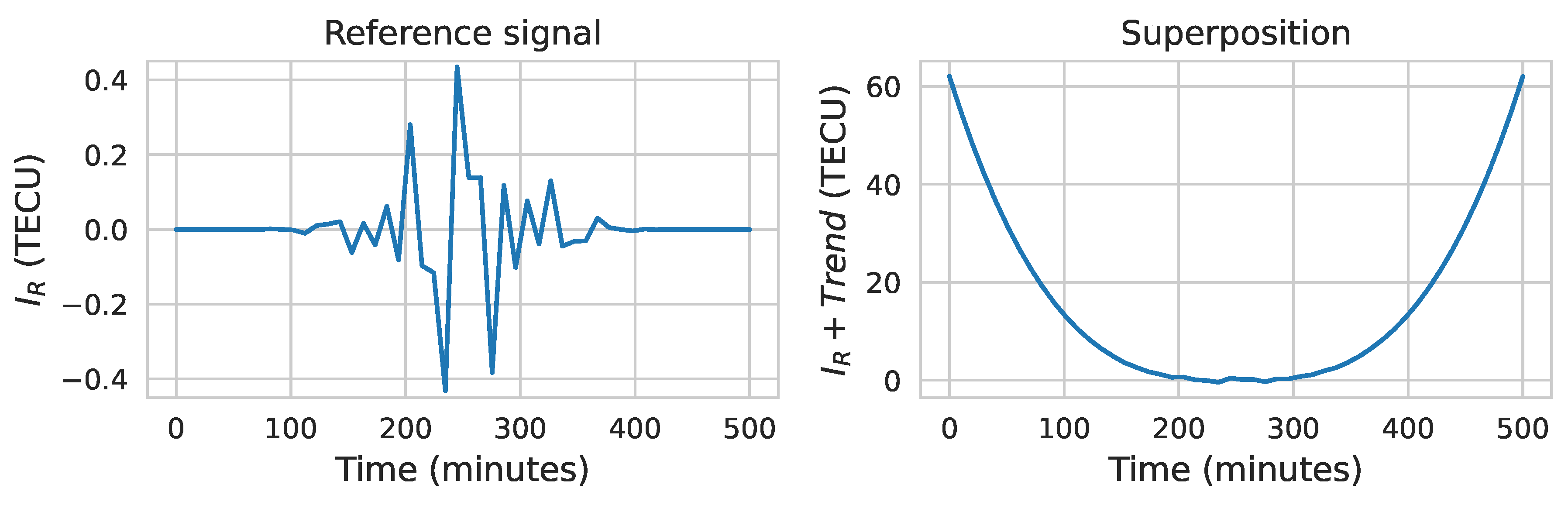
Where equation (A6) is the signal to detrend, and equation (A7) is the trend to remove. A is the amplitude of the signal, set as 0.2 TECU, is a parameter which determines the position of the envelope maximum, set as 250 min, which is the half of the array length, is the half width of the envelope, set as 50 min and are the frequencies of three harmonics with periods of 20 min, 40 min and 60 min. Besides, B is the amplitude of the trend, set as 3.84 × 10⁻⁶ and = 250 min determines position of the minimum of the trend.
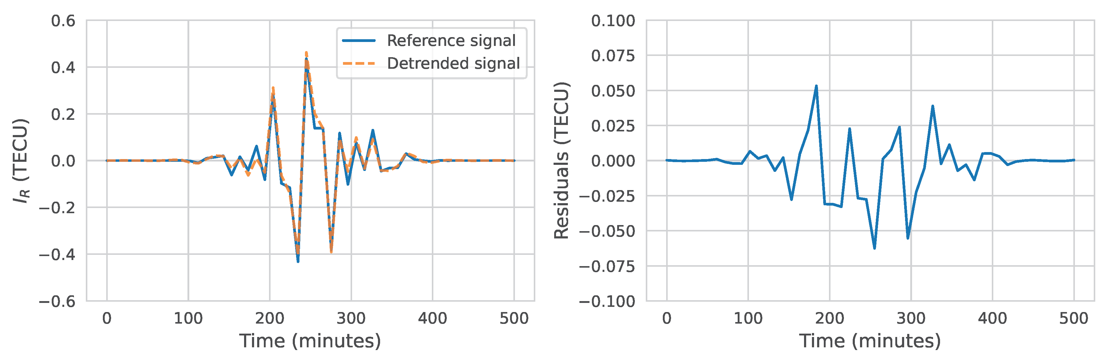
For the detrending, we used a Savitsky-Golay filter of order 3, this is lowest order filter which at the same time avoids too much oscillations and allows to the fit (and its derivative) to be smooth. The other remaining parameter is the window size, i.e. the number of convolution coefficients neccesary for the regression, which must be an odd integer, greater than the order of the polynomial order and lower than the array size. Then, we estimated the detrended signal using all possible values for the window size and estimated the residuals as follows:
Where N is the array size, is the value of the detrended signal at the time and is the reference signal at the same time. In Figure A2 we show the behavior of residuals as a function of the window size relative to the array size. We noted that the residuals behavior is almost insensitive to the window size when its size is lower than than 60% of the array size, when the errors start to grow exponentially, but going to more detail, we found that using a window size of about of the array length, such errors are minimal. The detrended test curve is shown in Figure A2, compared with the original signal, as well as the substraction of both curves. In the ideal case, it should be zero for all times, but even in this case the amplitude of the envelope is about the tenth part of the amplitude of the envelope of the signal.
Figure A2.
Left: Original test signal (blue continuous curve) compared with the result of detrending the superposition of the test signal with the test trend (rigth panel of Figure A1, which is the orange dashed curve. Right: Substraction of both curves of left side. The amplitude of the envelope of this residuals qualitatively is about tenth percent of the amplitude of the original signal.
Appendix C. UNAVCO Stations List
In Table A1 we enlist the stations from we collected data for our work, their coordinates and add the citation link when available, they are separated by sets, as shown in Figure 12. Stations in set 1 are all located in Dominican Republic, set 2 in the northern lesser antilles. Set 3 in the southern lesser antilles, set4 in Aruba, Curaçao and Trinidad and Tobago, and finally set 5 in continental land in Suriname and French Guyana. Stations highlighted in green are the ones where we suspect that TIDs were detected.

Table A1.
List of GNSS stations used for this work, classified in sets according to their spatial location. In highlighted stations at least in one of the satellite-receiver line of sight TIDs were detected.
Table A1.
List of GNSS stations used for this work, classified in sets according to their spatial location. In highlighted stations at least in one of the satellite-receiver line of sight TIDs were detected.
| Station name | Latitude (deg) | Longitude (deg) | Resolution data | Citation |
| Set 1 | ||||
| BARA | 18.21 | -71.09 | 15 s, 1Hz | None available |
| CN05 | 18.56 | -68.35 | 15 s, 1 Hz | https://doi.org/10.7283/T5VQ30ZH |
| CN27 | 19.67 | -69.93 | 15 s, 1 Hz | https://doi.org/10.7283/T5JD4V2P |
| CRLR | 18.41 | -68.93 | 15 s, 1 Hz | https://doi.org/10.7283/T5FN14JM |
| CRSE | 18.76 | -69.04 | 15 s | None available |
| JME2 | 18.23 | -72.54 | 15 s, 1 Hz | https://doi.org/10.7283/T5KW5D38 |
| LVEG | 19.22 | -70.53 | 15s, 1 Hz | https://doi.org/10.7283/T5CZ35GC |
| RDAZ | 18.45 | -70.72 | 15 s | None available |
| RDF2 | 19.45 | -70.68 | 15 s | None available |
| RDHI | 18.60 | -68.72 | 15 s | None available |
| RDLT | 19.31 | -69.55 | 15 s, 1 Hz | https://doi.org/10.7283/T5J101GT |
| RDMA | 19.54 | -71.08 | 15 s, 1 Hz | https://doi.org/10.7283/T50863NM |
| RDMC | 19.85 | -71.64 | 15 s, 1 Hz | None available |
| RDMS | 18.98 | -69.04 | 15 s | https://doi.org/10.7283/T5DV1HPQ |
| RDNE | 18.50 | -71.42 | 15 s | None available |
| RDSD | 18.46 | -69.91 | 15 s, 1 Hz | https://doi.org/10.7283/T5CZ3594 |
| RDSF | 19.29 | -70.25 | 15 s | None available |
| RDSJ | 18.82 | -71.23 | 15 s, 1 Hz | https://doi.org/10.7283/T59W0CTW |
| SPED | 18.46 | -69.31 | 15 s, 1 Hz | https://doi.org/10.7283/T5HQ3X75 |
| SROD | 19.48 | -71.34 | 15 s, 1 Hz | https://doi.org/10.7283/T5862DSD |
| TGDR | 18.21 | -71.10 | 15 s, 1 Hz | https://doi.org/10.7283/T5222S3R |
| Set 2 | ||||
| AIRS | 16.74 | -62.21 | 15 s | https://doi.org/10.7283/T53B5XGJ |
| CN00 | 17.67 | -61.79 | 15 s, 1 Hz | https://doi.org/10.7283/T5FN14GQ |
| GERD | 16.80 | -62.19 | 15 s | https://doi.org/10.7283/T5TT4PBT |
| NWBL | 16.82 | -62.20 | 15 s | https://doi.org/10.7283/T5ZK5F13 |
| OLVN | 16.75 | -62.23 | 15 s | https://doi.org/10.7283/T5Q23XMD |
| RCHY | 16.70 | -62.15 | 15 s | https://doi.org/10.7283/T5707ZSJ |
| RDON | 16.93 | -62.35 | 15 s | https://doi.org/10.7283/T5W37TFB |
| TRNT | 16.76 | -62.16 | 15 s | https://doi.org/10.7283/T5K935W2 |
| Set 3 | ||||
| CN04 | 14.02 | -60.97 | 15 s | https://doi.org/10.7283/T5BP0124 |
| GRE1 | 12.22 | -61.64 | 15 s | https://doi.org/10.7283/T5BC3WZ5 |
| Set 4 | ||||
| CN19 | 12.61 | -70.04 | 15 s | https://doi.org/10.7283/T5HD7SZB |
| CN40 | 12.18 | -68.96 | 15 s, 1 Hz | https://doi.org/10.7283/T5BV7DWT |
| TTSF | 10.28 | -61.47 | 15 s | https://doi.org/10.7283/T5JQ0ZCJ |
| TTUW | 10.64 | -61.40 | 15 s | https://doi.org/10.7283/T5TQ5ZTR |
| Set 5 | ||||
| BOAV | 2.85 | -60.70 | 15 s | None available |
| KOUG | 5.10 | -52.64 | 30 s | None available |
| KOUR | 5.25 | -52.81 | 30 s | None available |
References
- Dudorov, A.E.; Eretnova, O.V. The Rate of Falls of Meteoroids and Bolides. Solar System Research 2020, 54, 223–235. [Google Scholar] [CrossRef]
- Gutierrez-Zalapa, R.; Rodríguez-Martínez, M.; Aguilar-Rodríguez, E.; Estevez-Delgado, J. Modeling the impact of asteroids over Mexican territory. Revista Mexicana de Física 2024, 70, 010701–1. [Google Scholar] [CrossRef]
- Wheeler, L.F.; Mathias, D.L. Probabilistic assessment of Tunguska-scale asteroid impacts. Icarus 2019, 327, 83–96. [CrossRef]
- Yang, Y.M.; Komjathy, A.; Langley, R.B.; Vergados, P.; Butala, M.D.; Mannucci, A.J. The 2013 Chelyabinsk meteor ionospheric impact studied using GPS measurements. Radio Science 2014, 49, 341–350. [Google Scholar] [CrossRef]
- DOF. DECRETO por el que se reforman los articulos 2 y 82; y se adicionan la fraccion XXI del articulo 2, recorriendo el orden de las fracciones subsecuentes, y un segundo y tercer parrafos al articulo 20 de la Ley General de Proteccion Civil.; Diario Oficial de la Federación, 6 de junio de 1994., 2014.
- UNDRR. Hazard definition and classification review: Technical report.; United Nations Office for Disaster Risk Reduction International Science Council (ISC), 2020.
- Savitzky, A.; Golay, M.J. Smoothing and differentiation of data by simplified least squares procedures. Analytical chemistry 1964, 36, 1627–1639. [Google Scholar] [CrossRef]
- Chernogor, L. Ionospheric effects of the Chelyabinsk meteoroid. Geomagnetism and Aeronomy 2015, 55, 353–368. [Google Scholar] [CrossRef]
- Maruyama, T.; Kato, H.; Nakamura, M. Ionospheric effects of the Leonid meteor shower in November 2001 as observed by rapid run ionosondes. Journal of Geophysical Research: Space Physics 2003, 108. [Google Scholar] [CrossRef]
- Kelley, M.C. The Earth’s ionosphere: Plasma physics and electrodynamics; Academic press, 2009.
- Tsugawa, T.; Saito, A.; Otsuka, Y. A statistical study of large-scale traveling ionospheric disturbances using the GPS network in Japan. Journal of Geophysical Research: Space Physics 2004, 109. [Google Scholar] [CrossRef]
- Afraimovich, E.L.; Astafyeva, E.I.; Demyanov, V.V.; Edemskiy, I.K.; Gavrilyuk, N.S.; Ishin, A.B.; Kosogorov, E.A.; Leonovich, L.A.; Lesyuta, O.S.; Palamartchouk, K.S.; others. A review of GPS/GLONASS studies of the ionospheric response to natural and anthropogenic processes and phenomena. Journal of Space Weather and Space Climate 2013, 3, A27. [Google Scholar] [CrossRef]
- Goodman, S.J.; Blakeslee, R.J.; Koshak, W.J.; Mach, D.; Bailey, J.; Buechler, D.; Carey, L.; Schultz, C.; Bateman, M.; McCaul, E.; Stano, G. The GOES-R Geostationary Lightning Mapper (GLM). Atmospheric Research 2013, 125-126, 34–49. [Google Scholar] [CrossRef]
- Ogwala, A.; Somoye, E.O.; Ogunmodimu, O.; Adeniji-Adele, R.A.; Onori, E.O.; Oyedokun, O. Diurnal, seasonal and solar cycle variation in total electron content and comparison with IRI-2016 model at Birnin Kebbi. Annales Geophysicae 2019, 37, 775–789. [Google Scholar] [CrossRef]
- Maletckii, B.; Yasyukevich, Y.; Vesnin, A. Wave Signatures in Total Electron Content Variations: Filtering Problems. Remote Sensing 2020, 12. [Google Scholar] [CrossRef]
- Pradipta, R.; Valladares, C.E.; Doherty, P.H. An effective TEC data detrending method for the study of equatorial plasma bubbles and traveling ionospheric disturbances. Journal of Geophysical Research: Space Physics 2015, 120, 11048–11055. [Google Scholar] [CrossRef]
- Savitzky, A.; Golay, M.J.E. Smoothing and differentiation of data by simplified least squares procedures. Analytical Chemistry 1964, 36, 1627–1639. [Google Scholar] [CrossRef]
- Romero-Hernandez, E.; Salinas-Samaniego, F.; Jonah, O.F.; Aguilar-Rodriguez, E.; Rodriguez-Martinez, M.; da Silva Picanço, G.A.; Denardini, C.M.; Guerrero-Peña, C.A.; Aguirre-Gutierrez, R.; Garcia-Castillo, F.A.; others. Properties of Medium-Scale Traveling Ionospheric Disturbances Observed over Mexico during Quiet Solar Activity. Atmosphere 2024, 15, 894. [Google Scholar] [CrossRef]
- Xiao, Z.; Xiao, S.g.; Hao, Y.q.; Zhang, D.h. Morphological features of ionospheric response to typhoon. Journal of Geophysical Research: Space Physics 2007, 112. [Google Scholar] [CrossRef]
- Sergeeva, M.A.; Demyanov, V.V.; Maltseva, O.A.; Mokhnatkin, A.; Rodriguez-Martinez, M.; Gutierrez, R.; Vesnin, A.M.; Gatica-Acevedo, V.J.; Gonzalez-Esparza, J.A.; Fedorov, M.E.; others. Assessment of morelian meteoroid impact on Mexican environment. Atmosphere 2021, 12, 185. [Google Scholar] [CrossRef]
- D’Angelo, G.; Spogli, L.; Cesaroni, C.; Sgrigna, V.; Alfonsi, L.; Aquino, M. GNSS data filtering optimization for ionospheric observation. Advances in Space Research 2015, 56, 2552–2562. [Google Scholar] [CrossRef]
- Flynn, G.; Moore, L.; Klöck, W. Density and Porosity of Stone Meteorites: Implications for the Density, Porosity, Cratering, and Collisional Disruption of Asteroids. Icarus 1999, 142, 97–105. [Google Scholar] [CrossRef]
- Öpik, E.J. Physics of Meteor Flight in the Atmosphere. Interscience Publ. Inc.(New York) 1958, p. 147.
- Gutiérrez-Zalapa, R.; Rodriguez-Martinez, M.; Aguilar-Rodriguez, E.; Estevez-delgado, J.; Olguin, L. Modeling the transit of a NEO through the Earth’s atmosphere. 44th COSPAR Scientific Assembly. Held 16-24 July, 2022, Vol. 44, p. 229.
- Feng, C.; Zeng, X.; Li, Z.; Gan, Q. Atmospheric Entry and Strewn Fields Estimation for Rubble-pile Meteoroids. Advances in Space Research 2024. [Google Scholar] [CrossRef]
- Hills, J.G.; Goda, M.P. The fragmentation of small asteroids in the atmosphere. Astronomical Journal (ISSN 0004-6256), vol. 105, no. 3, p. 1114-1144. 1993, 105, 1114–1144. [Google Scholar] [CrossRef]
- Mathias, D.L.; Wheeler, L.F.; Dotson, J.L. A probabilistic asteroid impact risk model: assessment of sub-300 m impacts. Icarus 2017, 289, 106–119. [Google Scholar] [CrossRef]
- Somsikov, V.M. Solar terminator and dynamic phenomena in the atmosphere: A review. Geomagnetism and Aeronomy 2011, 51, 707–719. [Google Scholar] [CrossRef]
- Paul, K.; Haralambous, H.; Oikonomou, C. Rate of total electron content index (ROTI) characteristics over Cyprus. Tenth International Conference on Remote Sensing and Geoinformation of the Environment (RSCy2024). SPIE, 2024, Vol. 13212, pp. 183–190.
- Laštovička, J.; Šindelářová, T. Large-scale and transient disturbances and trends: from the ground to the ionosphere. Infrasound Monitoring for Atmospheric Studies: Challenges in Middle Atmosphere Dynamics and Societal Benefits 2019, pp. 777–804.
- Colestock, P.; Close, S.; Zinn, J. Theoretical and observational studies of meteor ionization with the atmosphere in characterizing the ionosphere. Meeting Proceedings RTO M.P. IST-056, 2006, pp. 12–1 to 12–12.
- Li, C.; Hancock, C.M.; Hamm, N.A.S.; Veettil, S.V.; You, C. Analysis of the Relationship between Scintillation Parameters, Multipath and ROTI. Sensors 2020, 20. [Google Scholar] [CrossRef] [PubMed]
- Su, K.; Jin, S.; Hoque, M.M. Evaluation of ionospheric delay effects on multi-GNSS positioning performance. Remote Sensing 2019, 11, 171. [Google Scholar] [CrossRef]
- Stankov, S.; Jakowski, N. Ionospheric effects on GNSS reference network integrity. Journal of Atmospheric and Solar-Terrestrial Physics 2007, 69, 485–499. [Google Scholar] [CrossRef]
| 1 |
Figure 1.
Upon entering Earth’s atmosphere over the Caribbean region on June 22, 2019, this small Near-Earth Object produced an intense flash. Image from the GOES satellite, RAMMB/CIRA/Colorado State University.
Figure 1.
Upon entering Earth’s atmosphere over the Caribbean region on June 22, 2019, this small Near-Earth Object produced an intense flash. Image from the GOES satellite, RAMMB/CIRA/Colorado State University.
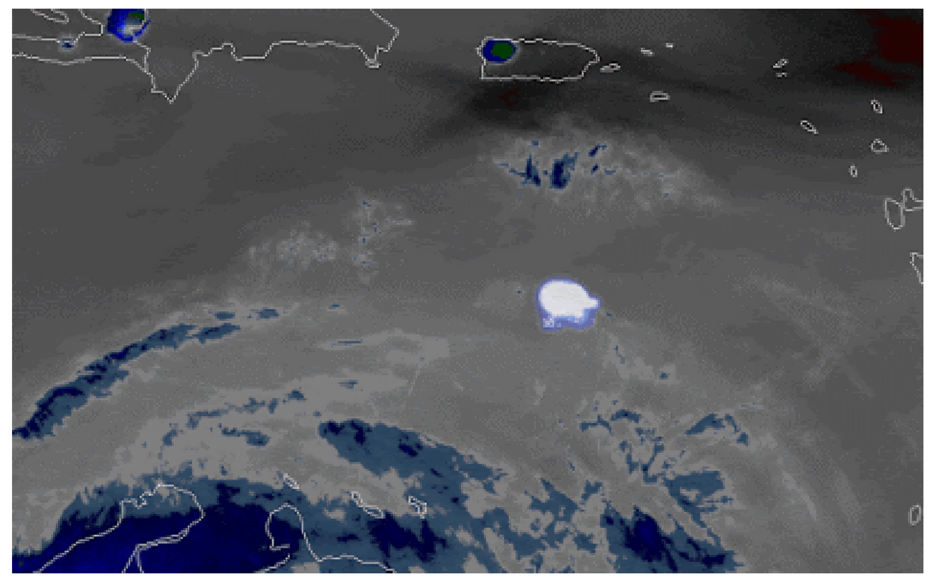
Figure 2.
Comparison between Yang et al. [4] reconstructed TEC series from coherence spectrum most prominent frequencies and sTEC series and our detrended data for ARTU-PRN18 (top row) and ARTU-PRN26 (bottom row) satellite-station links. In left panels we see the high frequencies time series, in middle panels the low frequencies time series and our detrended data in right panels.
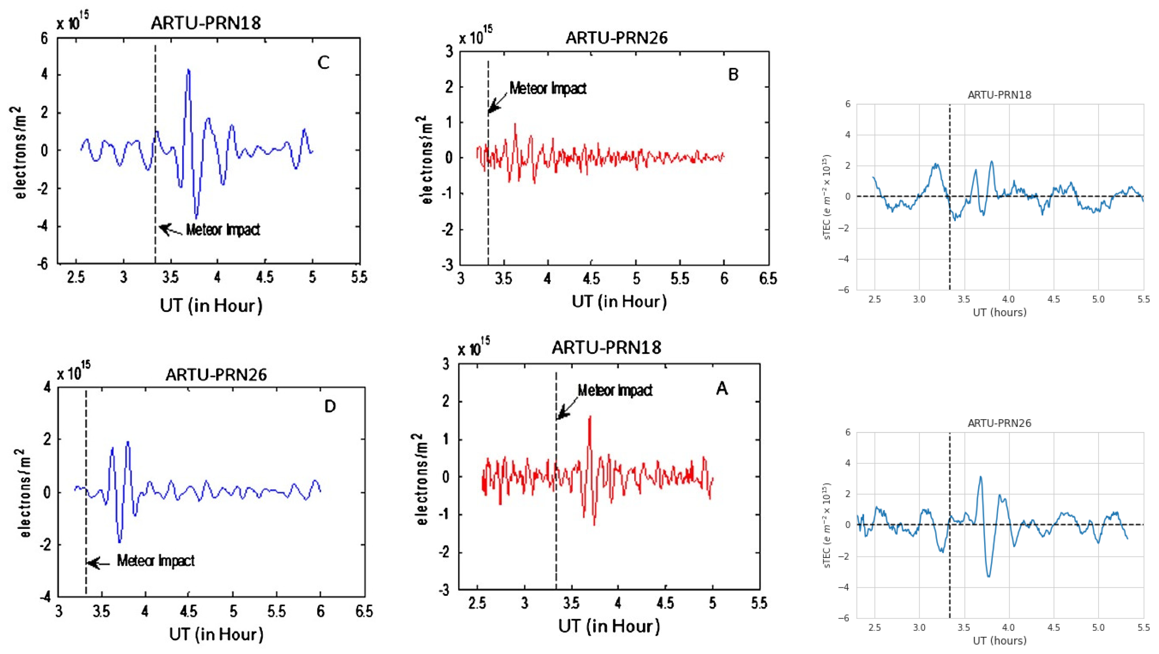
Figure 3.
Solutions of flight equations following Gutiérrez-Zalapa et al. [24] which models the dynamics of the meteor as it passes through the Earth’s atmosphere. In the top panel we show the meteor velocity as a function of height. In the middle the mass and in the bottom the flight angle. The vertical dashed line indicates the height where fragmentation (or breakup) occurred, while the dot-dashed line represents the height where the most energy liberation occurred.
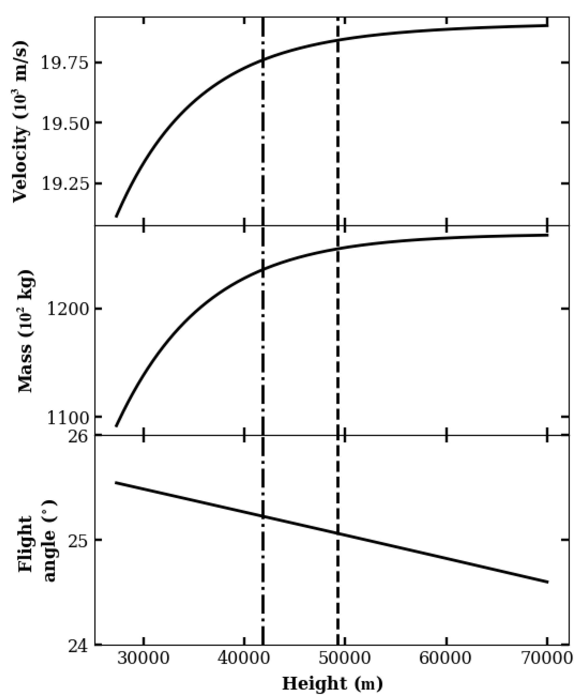
Figure 4.
Top panel: Meteor diameter as a function of height. After burst and breakup we consider the diameter of the fragmentation cloud mass, explaining the growth of this parameter at lower heights. Bottom panel: Meteor density as a function of height. Vertical lines and parameters at top panels are the same as Figure 3.
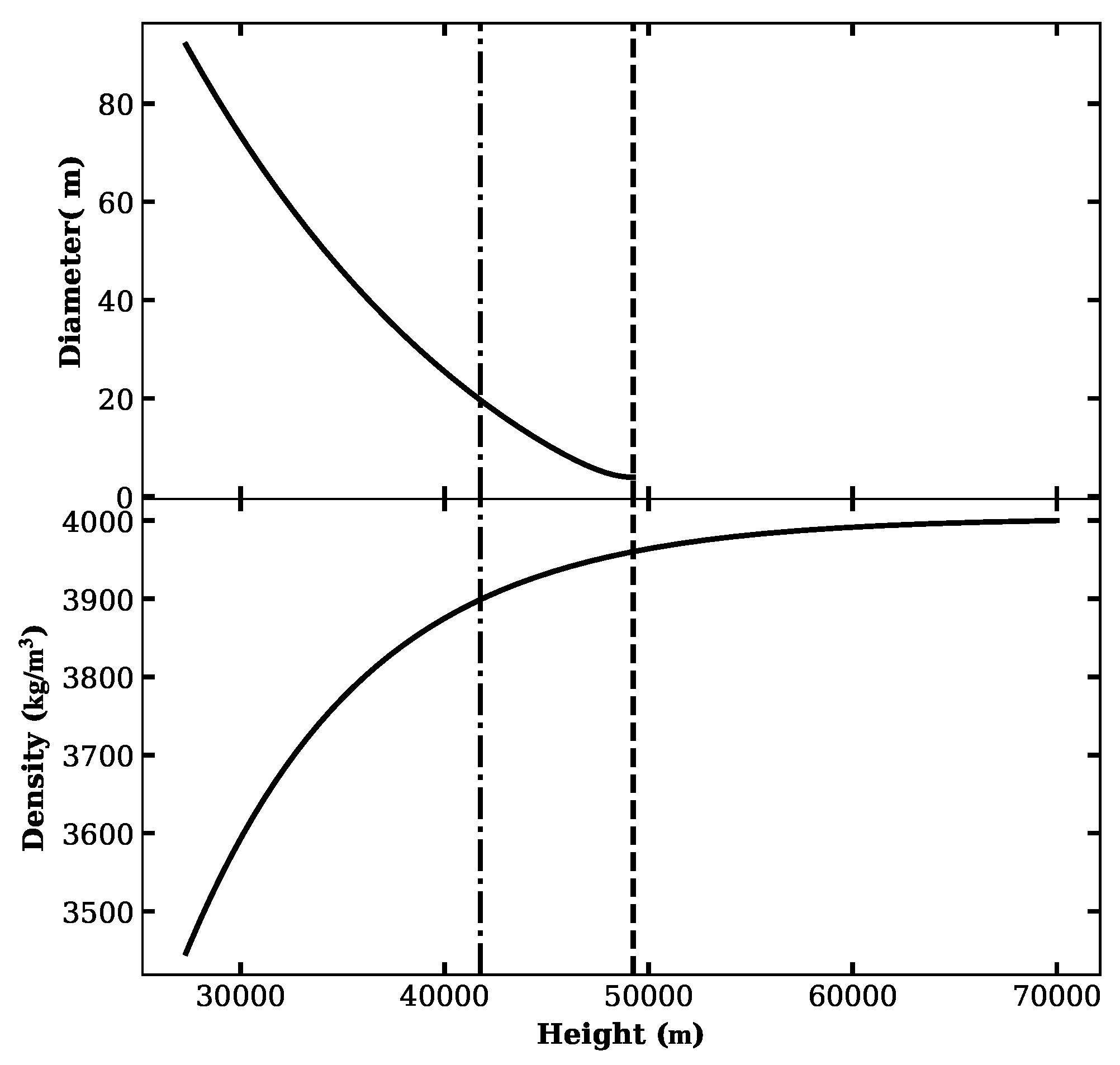
Figure 5.
In top panel we show the energy deposition as a function of height. Finally, at bottom we show the pressure versus height. The lower dotted line indicates the stagnation pressure of the meteor.
Figure 5.
In top panel we show the energy deposition as a function of height. Finally, at bottom we show the pressure versus height. The lower dotted line indicates the stagnation pressure of the meteor.
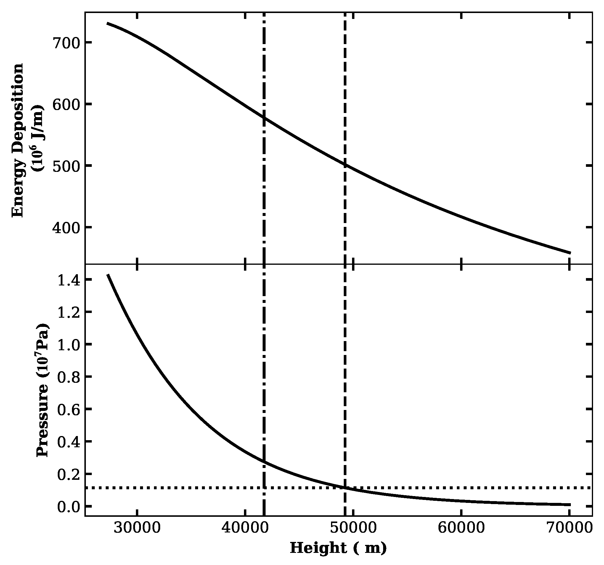
Figure 6.
Dst index for 2019 June 22th. Data obtained from WDC for Geomagnetism, Kyoto DST index service.
Figure 6.
Dst index for 2019 June 22th. Data obtained from WDC for Geomagnetism, Kyoto DST index service.
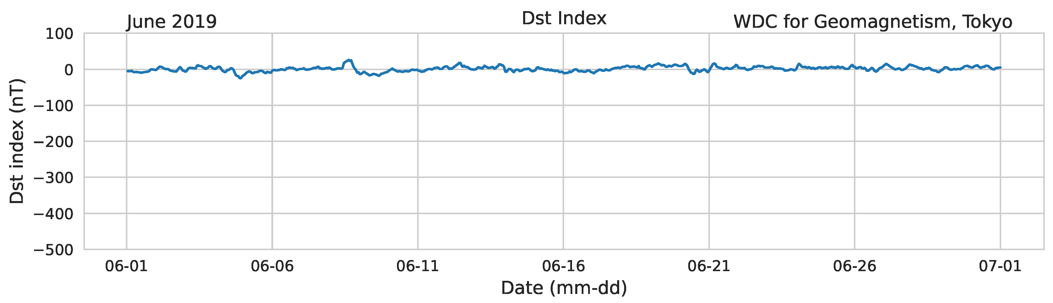
Figure 7.
Relative speed of solar wind at the event day and previous week respect the previous day, normalized with speed of sound. Each curve represents one day data.
Figure 7.
Relative speed of solar wind at the event day and previous week respect the previous day, normalized with speed of sound. Each curve represents one day data.
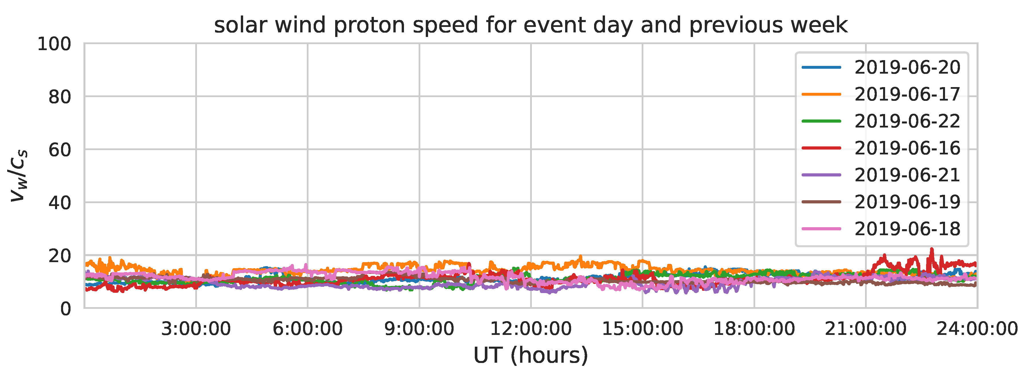
Figure 8.
Solar terminator position (orange line) for the most southern GNSS stations: BOAV, KOUG and KOUR, at the time detection (burst time) of 21:25:48 UTC, as it is indicated in Table 1. The stations KOUR and KOUG were situated at a distance of approximately 20 minutes from this line, at that moment. The meteoroid burst position is indicated with a green star.
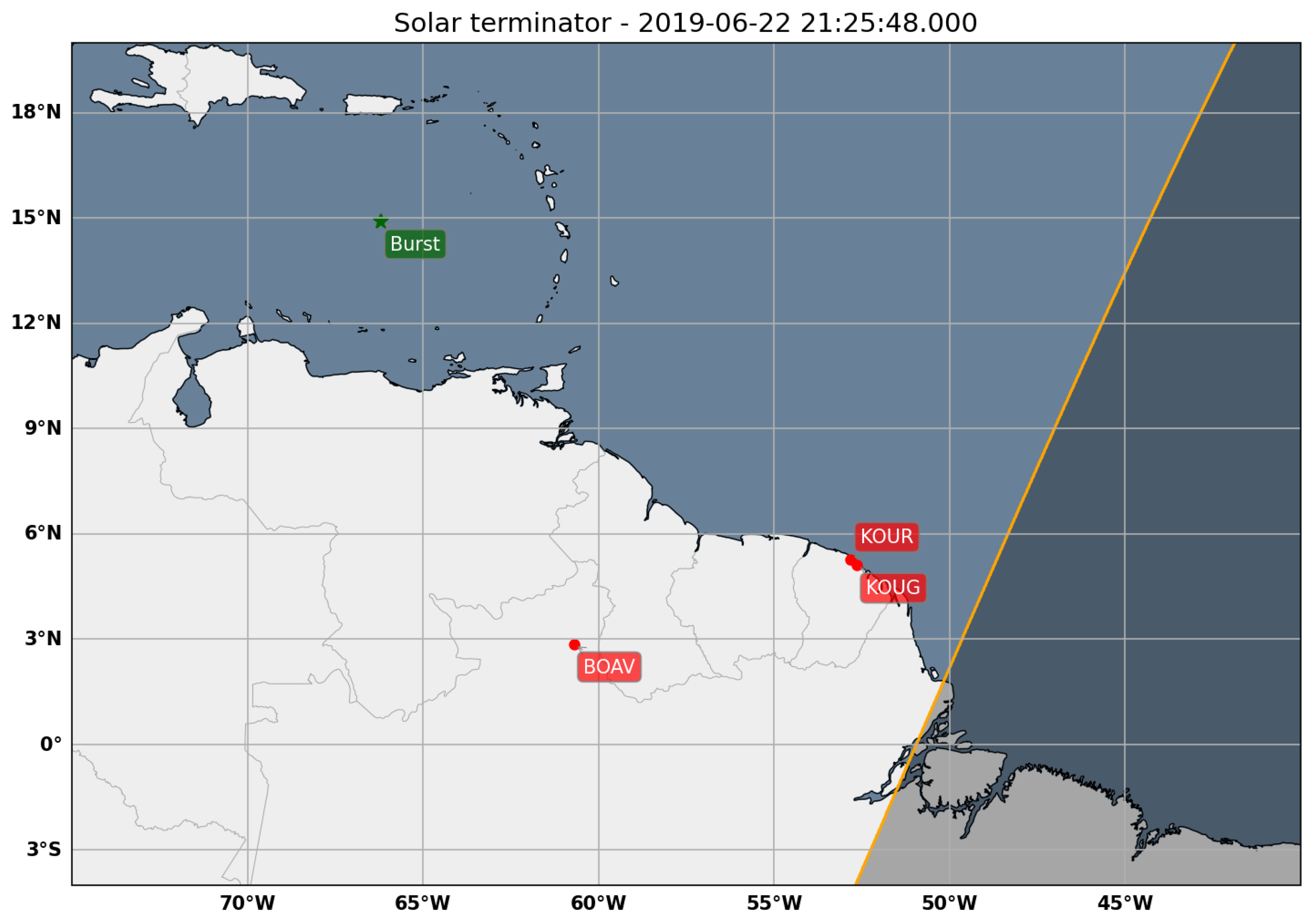
Figure 9.
Detrended sTEC time series for station KOUG for the days 2019-06-20, 2019-06-21 and 2019-06-22 (three and two days before meteor fall), and the meteor fall date, from left to right). The satellite receiver LOS with PRN 2 is in top, and the LOS with PRN 12 is in bottom.
Figure 9.
Detrended sTEC time series for station KOUG for the days 2019-06-20, 2019-06-21 and 2019-06-22 (three and two days before meteor fall), and the meteor fall date, from left to right). The satellite receiver LOS with PRN 2 is in top, and the LOS with PRN 12 is in bottom.
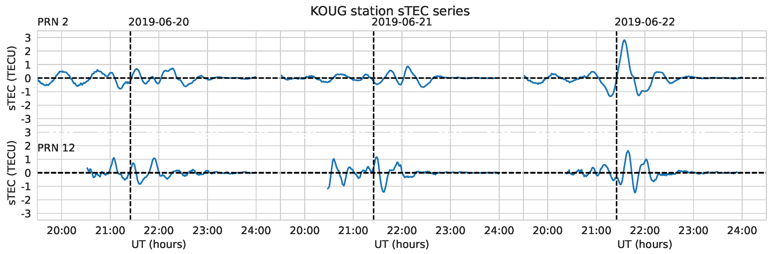
Figure 10.
sTEC time series for stations where TIDs are likely to be detected. We show the time series for the previous day of meteor fall, and the time series for the meteor fall (dashed line) date. We show sTEC time series for stations CN04 (which belong to set 3), CN40, TTSF and TTUW (set 4)
Figure 10.
sTEC time series for stations where TIDs are likely to be detected. We show the time series for the previous day of meteor fall, and the time series for the meteor fall (dashed line) date. We show sTEC time series for stations CN04 (which belong to set 3), CN40, TTSF and TTUW (set 4)
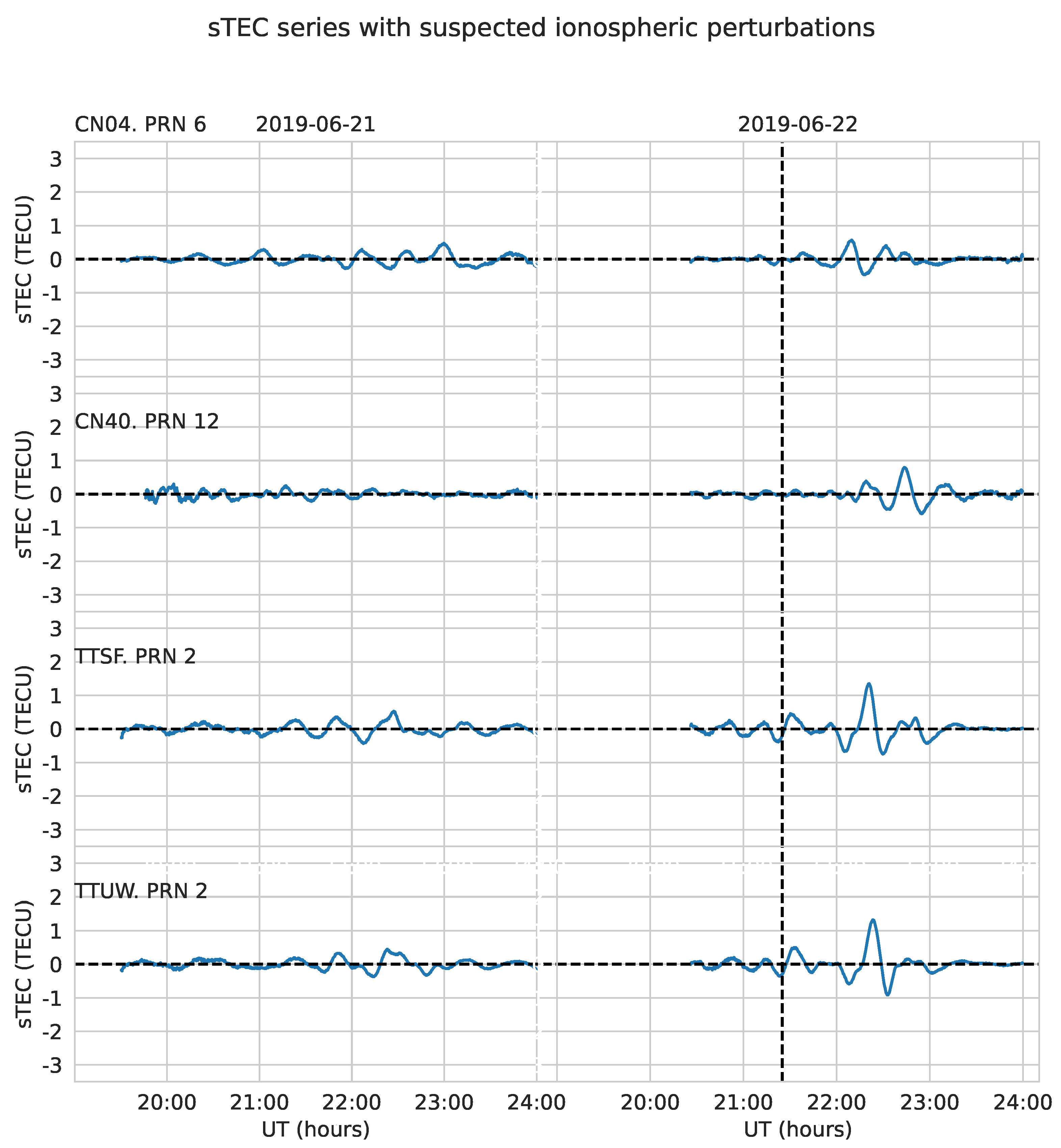
Figure 11.
Continuation of Figure 10, showing the station GRE! (set 3) and stations BOAV and KOUG (set 5).
Figure 11.
Continuation of Figure 10, showing the station GRE! (set 3) and stations BOAV and KOUG (set 5).
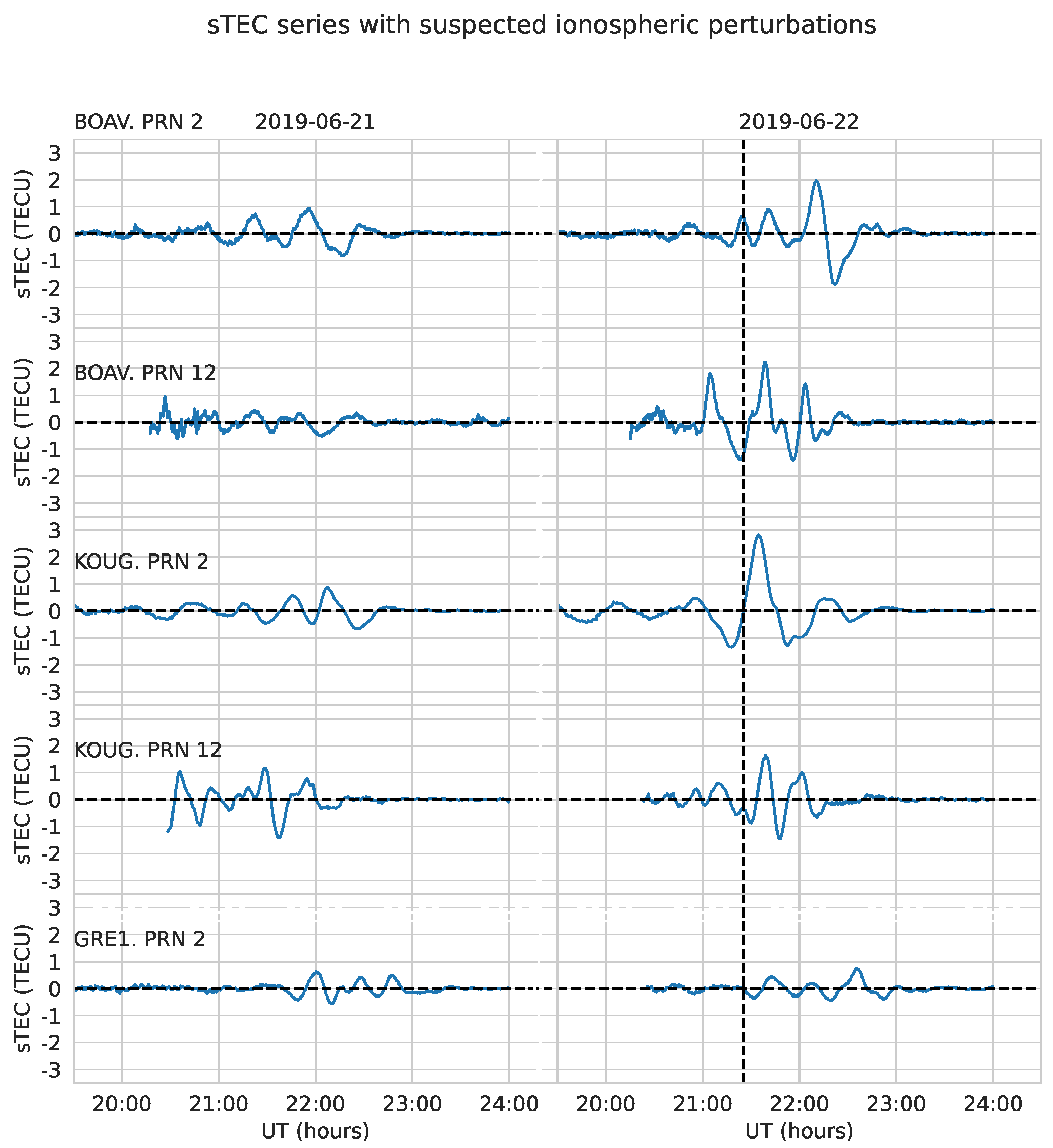
Figure 12.
Distribution of UNAVCO stations positions. We classified such stations into 5 sets, roughly based in their locations, but mainly for organizational purposes. The red star is the position of the meteor reported by the USG sensors, the magenta dots corresponds with the GLM data. The green dashed line corresponds to the meteor estimated trajectory using the solutions of the flight equations from Gutiérrez-Zalapa et al. [24] shown in Figure 3, Figure 4 and Figure 5, the green star marks the position when breakup started. The red dashed line is an extrapolation back in time until the meteor crossed through the IPP, marked with the blue star, where presumably the meteor first perturbed the ionosphere. The upper left graph is a zoom of the region within the gray rectangle.
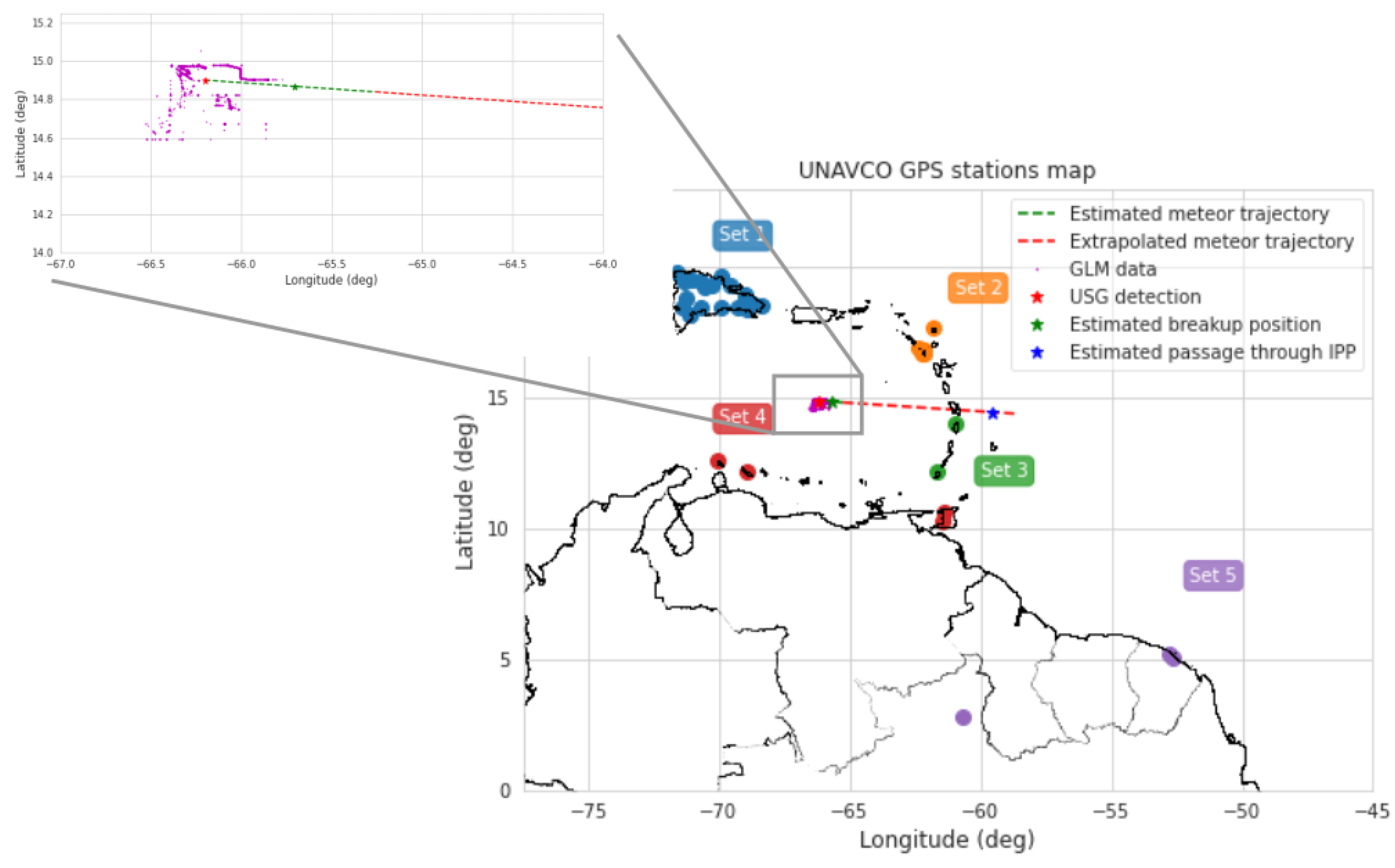
Figure 13.
Left: ROTI estimations with CN40 station data with different satellites. Right: detrended TEC for the same data.
Figure 13.
Left: ROTI estimations with CN40 station data with different satellites. Right: detrended TEC for the same data.
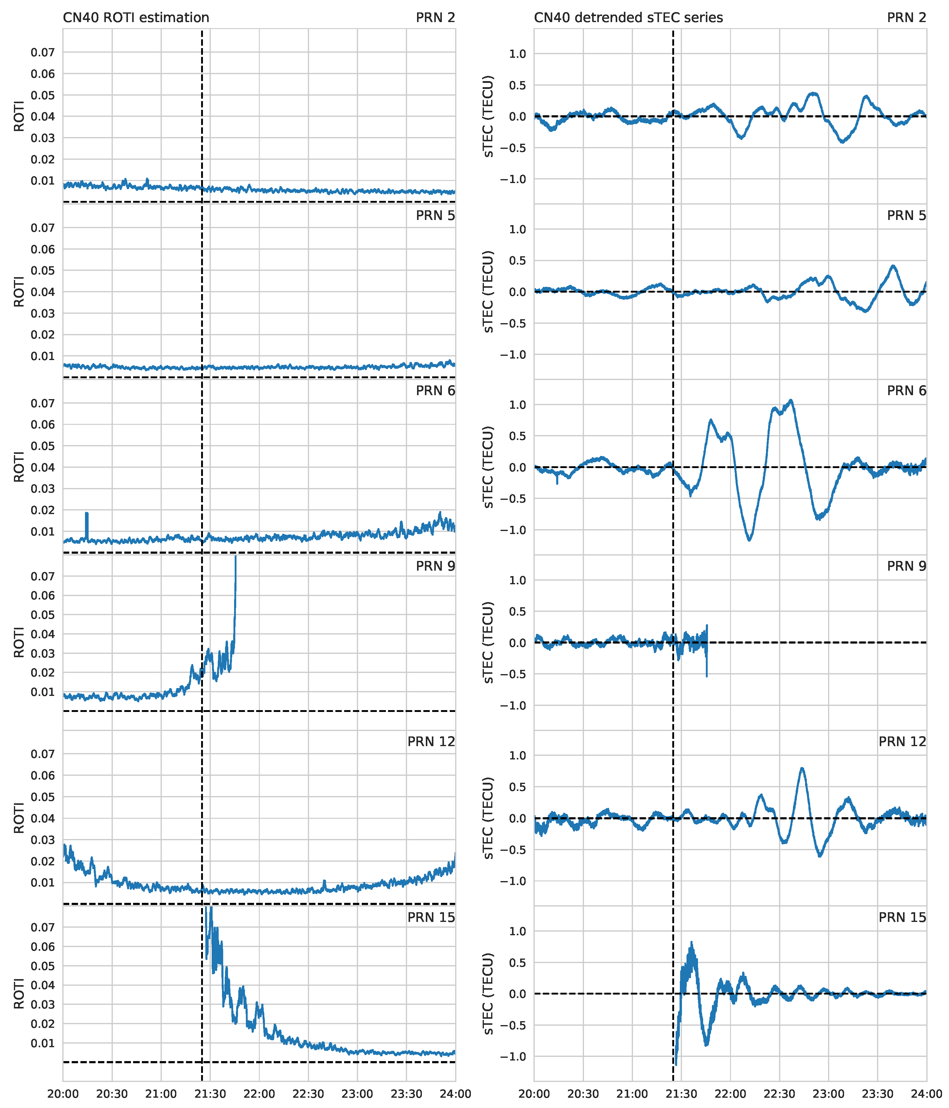
Table 1.
List of meteor basic parameters, compared with Chelyabinsk meteor event. Source: https://cneos.jpl.nasa.gov/fireballs/.
Table 1.
List of meteor basic parameters, compared with Chelyabinsk meteor event. Source: https://cneos.jpl.nasa.gov/fireballs/.
| Caribbean meteor | Chelyabinsk meteor | ||
| Date (DD Month YYYY) | 22 June 2019 | 15 February 2013 | |
| Time (UT) | 21:25:48 | 03:20:33 | |
| Latitude (deg) | 14.9 | 54.8 | |
| Longitude (deg) | -66.2 | 61.1 | |
| Altitude (km) | 25.0 | 23.3 | |
| Velocity (km/s) | 14.96 | 18.6 | |
| Duration (seconds) | 4.873 | ||
| -13.4 | 12.8 | ||
| Velocity components (km s−1) | 6.0 | -13.3 | |
| 2.5 | -2.4 | ||
| Total radiated energy (J) | 294.7 × 10¹⁰ | 3.75 × 10¹⁴ | |
| Calculated Total Impact energy (kt) | 6 | 440 |
Notes – Row. (1): Meteoroid fell date, in format DD Month YYYY. Row. (2): Detection time (UT), in format hh:mm:ss, for the burst. Row. (3): Latitude of meteoroid at detection time, in degrees. Row. (4): Longitude of meteoroid at detection time, in degrees. Row. (5): Estimated meteoroid velocity, in km s−1 Row. (6)†: Duration of meteoroid detection, in seconds. Row. (7)-(9): Meteoroid velocity components. Row (7) is for the velocity in the equatorial plane, positive towards the prime meridian. Row (9) is for the velocity directed towards the celestial north pole and row (8) completes the right-handed coordinate system. Row. (10): Meteoroid total radiated energy, in joules. Row. (11): Meteoroid total kinetic energy, in kilotons. †:Source: https://neo-bolide.ndc.nasa.gov/#/
Table 2.
Caribbean meteor possible physical initial parameters obtained by solving flight equations [24], assuming an initial density of 4000 kg m−3.
Table 2.
Caribbean meteor possible physical initial parameters obtained by solving flight equations [24], assuming an initial density of 4000 kg m−3.
| Initial Velocity | 19.9 km s−1 |
| Initial mass (×105) | 1.3 kg |
| Entry angle (deg) | 24.6 |
| Diameter | 3.9 m |
Table 3.
Numerical values extracted from the results of the solutions for the flight equations near the breakup instant. These values are necessary to estimate the meteor trajectory as it passed through the atmosphere.
Table 3.
Numerical values extracted from the results of the solutions for the flight equations near the breakup instant. These values are necessary to estimate the meteor trajectory as it passed through the atmosphere.
| UT | Height (km) | Velocity (km s−1) | Trajectory angle (deg) |
| 21 h 25 m 42.5 s | 70 | 20.60 | 24.60 |
| 21 h 25 m 43.7 s | 60 | 20.60 | 24.82 |
| 21 h 25 m 44.8 s | 50 | 20.50 | 25.04 |
| 21 h 25 m 46.0 s | 40 | 19.50 | 25.26 |
| 21 h 25 m 47.3 s | 30 | 16.50 | 25.50 |
| 21 h 25 m 48.0 s | 25 | 15.00 | 25.62 |
Disclaimer/Publisher’s Note: The statements, opinions and data contained in all publications are solely those of the individual author(s) and contributor(s) and not of MDPI and/or the editor(s). MDPI and/or the editor(s) disclaim responsibility for any injury to people or property resulting from any ideas, methods, instructions or products referred to in the content. |
© 2024 by the authors. Licensee MDPI, Basel, Switzerland. This article is an open access article distributed under the terms and conditions of the Creative Commons Attribution (CC BY) license (http://creativecommons.org/licenses/by/4.0/).
Copyright: This open access article is published under a Creative Commons CC BY 4.0 license, which permit the free download, distribution, and reuse, provided that the author and preprint are cited in any reuse.


