
Submitted:
24 December 2024
Posted:
26 December 2024
You are already at the latest version
Abstract
Solar eclipses present a valuable opportunity for controlled in-situ ionosphere studies. This work explores the response of the upper atmosphere’s F-layer during the total eclipse of April 8, 2024, which was primarily visible across North and South America. Employing a multi-instrument approach, we analyze the impact on the ionosphere’s Total Electron Content (TEC) and Very Low Frequency (VLF) signals over a three-day period encompassing the eclipse (April 7 to 9, 2024). Ground-based observations leverage data from ten strategically positioned International GNSS Service (IGS)/Global Positioning System (GPS) stations and four VLF stations situated along the eclipse path. We compute vertical TEC (VTEC) alongside temporal variations in VLF signal amplitude and phase to elucidate the ionosphere’s response. Notably, IGS station data reveal a decrease in VTEC during the partial and total solar eclipse phases, signifying a reduction in ionization. While VLF data also exhibit a general decrease, they display more prominent fluctuations. Space-based observations incorporate data from Swarm and COSMIC2 satellites as they traversed the eclipse path. Additionally, a spatiotemporal analysis utilizes data from the Global Ionospheric Map (GIM) database and the DLR’s (The German Aerospace Center’s) database. All space-based observations consistently demonstrate a significant depletion in VTEC during the eclipse. We further investigate the correlation between the percentage change in VTEC and the degree of solar obscuration, revealing a positive relationship. The consistent findings obtained from this comprehensive observational campaign bolster our understanding of the physical mechanisms governing ionospheric variability during solar eclipses. The observed depletion in VTEC align with the established principle that reduced solar radiation leads to decreased ionization within the ionosphere. Finally, geomagnetic data analysis confirms that external disturbances did not significantly influence our observations.
Keywords:
Solar Eclipse
; Vertical Total Electron Content
; VLF Radio Wave
; Multi-instrument Observations
; Global Ionospheric Map
1. Introduction
The ionosphere, a region of the Earth’s upper atmosphere spanning approximately 48 km to 965 km in altitude, plays a pivotal role in the celestial theater of solar eclipses. This dynamic layer, composed of ionized particles influenced by solar radiation, is the canvas that unfolds the intricate interplay between the Earth, Moon, and Sun. At the heart of this cosmic spectacle resides the solar eclipse. As the Moon orbits elliptically around our planet, it periodically aligns perfectly with the Sun, casting its shadow upon the Earth’s surface. This alignment results in a temporary obscuration of the solar disk, known as an eclipse, which can manifest as either a partial, total, or annular eclipse depending on the precise alignment and relative distances of the Earth, Moon, and Sun. While the visual spectacle of a solar eclipse enthralls observers on the ground, the ionosphere silently orchestrates a symphony of electromagnetic interactions integral to the event’s broader dynamics. During a solar eclipse, the abrupt reduction in solar radiance triggers rapid changes in the ionospheric electron density and temperature distribution. These fluctuations propagate throughout the ionosphere via complex ion-neutral coupling mechanisms, producing observable effects on radio wave propagation, atmospheric dynamics, and geomagnetic phenomena.
Moreover, the ionospheric response to a solar eclipse offers valuable insights into the underlying physical processes governing the Earth’s upper atmosphere. By analyzing the spatiotemporal evolution of ionospheric parameters during eclipses, we can refine existing models of ionospheric dynamics, elucidate the effects of solar variability on terrestrial climate, and enhance the accuracy of space weather forecasting [5,8,12,13]. This paper delves into the multifaceted relationship between the ionosphere and solar eclipses, exploring the mechanisms driving ionospheric disturbances during these celestial events and their broader implications for atmospheric science, space weather research, and telecommunications technology. Through a comprehensive synthesis of observational data, we aim to deepen our understanding of the ionospheric response to solar eclipses and its significance for Earth’s interconnected atmospheric system.
The ionosphere’s electron content is a vital parameter for understanding its behavior. Total Electron Content (TEC) measures the total number of electrons along a column from a satellite to a receiver on Earth. It is expressed in TEC Units (TECU), with 1 TECU corresponding to electrons/m2. On the other hand, Electron density in the ionosphere refers to the concentration of free electrons in a given volume of the Earth’s ionosphere. It is usually expressed in electrons per cubic meter (electrons/). The F2 layer, a key ionosphere region, is strongly linked to solar radiation. Its electron density rises after sunrise due to photo-ionization, peaking around noon or afternoon. As sunlight weakens, the F2 layer’s electron density diminishes after sunset. The ionosphere affects radio waves passing through it. Free electrons cause the waves to deviate from their original path. This is particularly important for the Global Positioning System (GPS), a key Global Navigation Satellite System (GNSS) component. When GPS signals travel through the ionosphere, they experience a delay directly proportional to TEC. We can study the Earth’s ionosphere by measuring TEC with dual-frequency GPS receivers. The UNAVCO Geodesy Advancing Geosciences and EarthScope (GAGE) Facility analyzes data from a network of over 2,000 GPS receivers. These continuously operating stations spread across North America, the Caribbean, and the high Arctic track Earth’s surface movement by recording position changes (time series) and velocities. Although GAGE’s primary focus is crustal motion, the data it collects can also be used to study the ionosphere’s TEC indirectly.
To analyze the impact of the solar eclipse on the ionosphere, we utilized data from the ESA’s Swarm satellite mission. The swarm consists of three satellites (Alpha, Bravo, and Charlie) launched in 2013 to study Earth’s magnetic field. Our study focused on data from the Swarm A satellite, which orbits at 470 km alongside another satellite (Swarm C). Previous research has documented the effects of solar eclipses on the ionosphere for decades [16,17][15,18]. This natural phenomenon offers a valuable opportunity to investigate how the Sun’s radiation influences the ionosphere-thermosphere-mesosphere (ITM) system [24]. This study specifically examined variations in and Electron density () during the total solar eclipse of April 8, 2024.
The Constellation Observing System for Meteorology, Ionosphere, and Climate-2/Formosa Satellite Mission 7 (COSMIC-2) GNSS Radio Occultation (RO) constellation, the successor to the successful COSMIC-1 program, consists of six identical micro-satellites. Each satellite carries a Tiny Ionospheric Photometer (TIP) and a Tri-Band-Beacon (TBB), which work together to enhance the accuracy and utility of ionospheric observations. These satellites orbit in six circular paths inclined at approximately and at an altitude of about 800 km, providing various measurements, including GPS-based RO data, to probe the Earth’s ionosphere and atmosphere. In this study, we observed the variation of the profile due to the total solar eclipse.
To compare and validate regional TEC models, global Vertical Total Electron Content () values are obtained from the Global Ionosphere Maps (GIM) provided by the International GNSS Service (IGS) network. GIM is an effective tool for studying the ionospheric response during seismic activity and solar eclipses. GIM data are available at 2 hours, 1 hour, 30 min, and 15 min.
The German Aerospace Center’s (DLR’s) global TEC maps offer detailed Vertical Total Electron Content (VTEC) data at an altitude of 400 km, significantly enhancing GNSS positioning accuracy compared to the Space Weather Application Center Ionosphere (SWACI) near real-time TEC map. Real-time GPS data from various sources by the German Federal Agency for Cartography and Geodesy in Frankfurt undergo preprocessing to derive calibrated slant TEC (STEC) values. These calibrated STEC values are then used to estimate coefficients for the Neustrelitz Total Electron Content Model (NTCM), which establishes the ionospheric background [33]. Integrating these measurements into the NTCM model allows for continuously updating a VTEC matrix every 5 minutes, with a spatial resolution of latitude by longitude. This matrix is stored in JSON format, ensuring users receive timely and accurate updates.
Radio waves emitted by VLF transmitters propagate within the waveguide formed by the lower ionosphere and the Earth’s surface. Significant variations in the amplitude and phase of the received signals are attributed to changes in the lower ionosphere. Previous studies have explored the analysis of the received VLF signals during eclipses, typically involving monitoring one to three transmitters (Tx) by one receiver (Rx). The first documented instance of an eclipse effect on VLF signals was reported by Bracewell et al. (1952) on the GBR (Tx in Rugby, England) to Cambridge (Rx) path during a partial eclipse in 1949. A notable change in phase was observed due to a 30% solar obscuration (Sun blockage). Studies focusing on short paths, defined as less than 1,000 km, have been infrequent but indicate amplitude increases of 2 or 3 dB and phase decreases ranging from to [2]. For medium paths ranging from 1,000 km to 10,000 km, Sen Gupta et al. (1980) documented that signal propagation characteristics undergo significant changes, including an increase in amplitude and a phase shift. Clilverd et al. (2001) presented findings from the total solar eclipse in Europe on August 11, 1999. Utilizing five receiving sets to monitor multiple stations, they analyzed 17 paths, varying in length from 90 km to 14,510 km. Their key observation was that for shorter propagation paths (<2,000 km), the amplitude change was positive, indicating signal enhancement, while for paths exceeding 10,000 km, the amplitude change was negative. Pal et al. (2012) examined the effects of the solar eclipse on July 22, 2009, on VLF signals across four propagation paths in the Indian subcontinent. Their observations revealed that, except for the VTX-Kolkata path, all other signals experienced a decrease in amplitude during the eclipse maximum. In this study, signals of the medium path from four transmitters were utilized: NPM at 21.4 kHz in Lualualei, Hawaii, USA; NAA at 24.0 kHz in Grimeton, Sweden; NLK at 24.8 kHz in Seattle, Washington, USA; and NML at 25.2 kHz in LaMoure, North Dakota, USA. Variations in the amplitude of the VLF signals recorded by a receiver located in rural SE Virginia, USA, were observed.
2. Materials and Methods
On April 8, 2024, a total solar eclipse occurred across North America, Canada, Mexico, and many countries in South and Central America. The partial eclipse began at 15:42 UTC and concluded at 20:52 UTC. The period of totality, during which the Moon completely obscured the Sun, was visible along a narrow path that stretched from Sinaloa to Coahuila in Mexico, from Texas to Maine in the United States, and from Ontario to Newfoundland in Canada. This totality phase started at 16:38 UTC and ended at 19:55 UTC.
In this manuscript, we investigate the ionospheric response to the total solar eclipse by analyzing four significant parameters: , , and the phase and amplitude of VLF signals. For computation, we employ five different methods: (a) IGS stations, (b) GIM database, (c) DLR database, (d) Swarm satellite data, and (e) Cosmic satellite data. Data were collected from six GNSS-IGS stations and four UNAVCO-IGS stations. Among the six GNSS-IGS stations, the total eclipse was observed from the IGS station NRC1, while the station INEG experienced a minimum obscuration of 90.67%. Among the four UNAVCO-IGS stations, the total eclipse was observed from station P777, with the station TNCU experiencing a minimum obscuration of 90.94%. Figure 1 illustrates the locations of the GNSS-IGS stations (marked with yellow diamonds) and the UNAVCO-IGS stations (marked with orange circles), as well as the totality belt (indicated by the red solid curve) spanning the North and South American landmasses.
The Receiver Independent Exchange Format (RINEX) observation and navigation files used for the computation of are sourced from the IGS data archive (https://cddis.nasa.gov/archive). measures the number of free thermal electrons (expressed in TECU) along a slant path between a satellite and a receiving station. A useful software has been developed by Gopi Seemala for all sorts of computations on , , satellite and receiver corrections, and bias and made accessible on the website (http://seemala.blogspot.com). The program code and its use for computation are mentioned in some important works [19,22]. We have attempted to convert the into an equivalent by using the thin shell approximation and using the technique given by [14,21,23,26,28,29].
The geometrical configuration of the Sun and the Moon during the eclipse, as suggested by [9], is shown in Figure 2(a). In Figure 2(b-d), we present the luminance and shadow spatiotemporal graph across the totality belt on the map. The luminance is calculated at the eclipse’s beginning, maximum, and end. Figure 2(b) shows the luminance at the start of the total solar eclipse on the totality belt. Similarly, Figure 2c and Figure 2d show the luminance during the middle and end of the total solar eclipse on the totality belt. In Figure 2(a), () and ) are the radii, and illustrated the centers of the Sun and Moon, respectively, as viewed from the central line of the eclipse shadow. This configuration illustrates the distance between their centers as observed from any shadow region of the Earth is D(). is the shadow region’s width along the centers’ joining line. The angle subtended by the point of intersection of the two perimeters and the centers of the Sun and the Moon is and . For the further computation of obscuration and luminance, we followed the calculation suggested by [9].
To analyze the influence of a solar eclipse on the ionosphere, we utilize data from NASA’s eclipse archive. This provides the coordinates of the eclipse path (latitude and longitude) as a function of time, defining the central line of the eclipse and its movement across Earth. Based on this path, we calculate the level of obscuration for various locations throughout the eclipse.
We compare the and data from the Swarm B satellite on the eclipse day (April 8, 2024) to a reference day within the same month to identify changes in the ionosphere caused by the eclipse. The reference day is selected to be a non-eclipse day that Swarm B satellite passed over the geographic longitude (W to W) between N and N at the same time (08:51 - 09:03 UT) as on the eclipse day. Only April 5, 2024, met this criterion. On the reference day, Swarm B satellite was above a similar region (W to W) from 09:43 to 09:55 UT. The data was accessed from https://vires.services on April 15, 2024. Using a combination of computation codes, we analyze the ionosphere’s response to the eclipse through and data and presented the results as a graph.
We further investigate variations during the eclipse using COSMIC-2 data. We compared the profiles on the eclipse day (April 8th, 2024) over the totality belt with a reference day (April 7th, 2024). To ensure a valid comparison, we selected COSMIC-2 data where the satellite passed over a similar geographic location and nearly the same time on both days. This data, accessed from the COSMIC-2 website https://www.cosmic.ucar.edu/what-we-do/cosmic-2/data on April 11th, 2024, is processed using established techniques, and the results are presented as a graph.
We present nine maps of ionospheric profiles along the path of totality using GIM data. For the computation of from the GIM database, we download the data for the eclipse day (April 8, 2024) and the non-eclipse days (April 7, 2024, and April 9, 2024) from 15:00 UTC to 20:00 UTC. Specifically, we focus on GIM data before the eclipse, during the maximum, and after the eclipse. The data is accessed from the website https://cddis.nasa.gov on April 12, 2024. A custom program is developed to analyze the collected raw data, enabling further observations and comparisons between the eclipse and non-eclipse periods. This approach allows for a detailed examination of how the solar eclipse influences ionospheric , providing insights into electron density dynamics during this celestial event.
To represent the DLR’s map, we display nine maps of ionospheric across the global map. The data is sourced from the website https://impc.dlr.de/SWE. The downloaded JSON file is then converted into a format suitable for further analysis. The resultant file undergo processing using code to plot the maps. To compare the variation of during the solar eclipse, we choose data from three consecutive days: the pre-eclipse day (April 7, 2024), the eclipse day (April 8, 2024), and the post-eclipse day (April 9, 2024). These maps provide a comprehensive visualization of the distribution and its variations along the path of totality during the eclipse period.
During the solar eclipse, we observe variations in the amplitude of the VLF signal at a receiver located in rural SE Virginia, USA, with coordinates N W and an elevation of 30 meters. The eclipse event at the receiver’s location evolved as follows: first contact occurred at 18:02:53 UT, the maximum eclipse intensity peaked at 19:19:19 UT with a magnitude of 0.834, and last contact was recorded at 20:31:48 UT. During this period, the center of totality was approximately 600 km NW of the receiver.
3. Results
The total solar eclipse was visible from Dallas, and its path spanned from Mexico’s Pacific coast to Newfoundland’s Atlantic coast, covering a narrow strip of the North American continent. While this path experienced totality, a partial solar eclipse was visible across North America, Central America, and Europe. We select six GNSS-IGS stations from these regions to study the temporal variation of during the eclipse (see Table 1). One station observed the total eclipse, while the other five observed partial eclipses. As shown in Table 1, all stations exhibited a depletion in the profile during the eclipse. Notably, station HLFX experienced the most significant reduction at 63.56%, while station INEG showed the least reduction at 18.09%. Station NRC1, which encountered 100% obscuration, recorded a depletion of 50.92%. Four stations experienced the eclipse during the forenoon hours, one at noon and one before noon. To illustrate the ionospheric response to the solar eclipse, we present three days of comparative profiles, including the mean of the non-eclipse days (April 7 and 9, 2024) and the eclipse day (April 8, 2024).
We also investigate the variations in the profiles across different UNAVCO-IGS stations. Data is collected from four stations (see Table 2), with one station experiencing a total solar eclipse while the others observe partial solar eclipses. As shown in Table 2, all stations recorded a depletion in profile. Station P777, experiencing 100% obscuration, showed a 25.95% decrement in profile during the solar eclipse. Stations SA56, P776, and TNCU, which observed partial solar eclipses with obscuration levels of 98.52%, 92.59%, and 90.94%, respectively, also experienced depletion in profile, with decreases of 54.84%, 59.36%, and 22.37%, respectively.
We explore the ionospheric response to the solar eclipse by analyzing the diurnal variation of the profile for each station, as mentioned above. We accomplish this by using three days of profiles: the eclipse day (April 8, 2024; DOY 99) and the two adjacent non-eclipse days (the days with Day of the Year –DOY– numbers 98 and 100, i.e., April 7, 2024, and April 9, 2024, respectively) from which a mean non-eclipse profile is calculated. Figure 3 and Figure 4, which follow the same format, illustrate the variation and percentage change in across three rows for each station, for the GNSS-IGS and the UNAVCO-IGS stations, respectively. Specifically, the first row shows the profile for three consecutive days, color-coded as follows: black for the pre-eclipse day (April 7, 2024; DOY 98), red for the eclipse day (April 8, 2024; DOY 99), and green for the post-eclipse day (April 9, 2024; DOY 100). The middle row displays the mean profile for the two non-eclipse days (black dashed curve) alongside the eclipse day profile (red solid curve). The last row depicts the variation in obscuration as a function of time at all stations (blue solid curve).
During the solar eclipse, we also observe changes in the electron density () profile. Utilizing data from Swarm-B satellite, collected during the same time frame and latitude-longitude as the profile data, Figure 5a illustrates the variation during the solar eclipse compared to a reference non-eclipse day. In the top row, the profiles for the eclipse day (red curve) and the non-eclipse day (black curve) are depicted across different latitudes with a fixed longitude. The second row displays the difference in profiles between the eclipse day and the selected quiet day. Correspondingly, the third row presents the percentage difference in profiles. Notably, the value decreases by 38% during the eclipse day. Additionally, Figure 5b provides the spatiotemporal variation of along with the trajectory of Swarm-B. In this figure, the first vertical line represents the satellite’s track on the reference day, while the second vertical line shows its track on the eclipse day. The red curve over the satellite’s tracks denotes the totality belt. From the color bar, it is clear that the electron density in the intersecting region is more intense on the reference day than on the eclipse day. Therefore, we conclude that the electron density during occultation decreases on the eclipse day.
Figure 5c presents a comparative analysis of the profile observed by the Swarm-B satellite during the eclipse and non-eclipse days. The top row illustrates the variation of profiles on the eclipse day (red) and the non-eclipse day (black) across different latitudes within a fixed longitude range. The middle panel highlights the difference in values (in TECU) between a reference day and the eclipse day. The third column depicts the percentage change in the profile between the eclipse and non-eclipse days, revealing a maximum depletion of approximately 22%. Additionally, Figure 5d presents the spatiotemporal variation of alongside the track of Swarm-B in the same region during the same time frame. In this figure, the first vertical line represents the satellite’s track on the reference day, while the second line shows its track on the eclipse day. The red curve superimposed on the satellite tracks delineates the path of totality. A comparative analysis of the color bar reveals a pronounced enhancement within the intersecting region during the reference day relative to the eclipse day.
Similarly, Figure 6 presents a comprehensive analysis of the profile during both eclipse and non-eclipse days, leveraging data from the COSMIC-2 satellite constellation. The top panel of Figure 6a visually shows the variation of profiles on eclipse (depicted in red) and non-eclipse days (depicted in black) across various latitudes and longitude ranges. The middle panel highlights the discrepancy in values (measured in electrons per cubic meter) between the reference day and the eclipse day. Notably, the third column illustrates the percentage change in the profile between the eclipse and non-eclipse days, revealing a maximum depletion of approximately 66%. Furthermore, the spatiotemporal dynamics of are illustrated, accompanied by the trajectory of the COSMIC-2 satellite during the almost same temporal window. This visualization demonstrates a significant depletion on the eclipse day relative to reference days.
The Swarm satellite data in the results only covers the partial eclipse phase, not the total eclipse. The depletion noted during this phase shows the effects of the partial eclipse, which may differ from those during the total eclipse. The Swarm satellite data during the total solar eclipse does not show any prominent changes because the data was collected before the eclipse started in the respective region. This implies that the signal does not capture the impact of the eclipse. While data is available for April 7 and 9, it does not meet the criteria relevant to the objective of this study. These dates do not align with the eclipse events that we are investigating, and thus, the data from these days does not contribute to the analysis.
Figure 7 showcases nine maps of ionospheric VTEC profiles along the eclipse path. For comparison, the first and third columns display VTEC variations on non-eclipse days (April 7 and 9, 2024). The second column showcases VTEC variations on the eclipse day (April 8, 2024) throughout the path, categorized by pre-, eclipse, and post-eclipse phases. Notably, a significant depletion in the VTEC profile is evident on eclipse days compared to non-eclipse days.
Similar to the GIM data, Figure 8 presents nine ionospheric VTEC maps for the computation of DLR’s data. These maps depict VTEC variations along the eclipse path. The first and third columns represent the VTEC profiles for the day before the eclipse (April 7, 2024) and the day after the eclipse (April 9, 2024), respectively, providing a reference for comparison. The second column showcases the VTEC variations specifically on the eclipse day (April 8, 2024). Here, the VTEC variations are further categorized into pre-eclipse, mid-eclipse and post-eclipse time periods to illustrate the changes throughout the totality belt.
Figure 9 illustrates a thorough analysis of the VLF amplitude profiles during eclipse and non-eclipse days. In each panel (corresponding to different paths), the top row presents the amplitude profiles for the eclipse day (red curve) and a non-eclipse day (black curve). The second row exhibits the difference in amplitude profiles between the eclipse day and the non-eclipse day. Correspondingly, the third row presents the degree of obscuration with respect to time. For this analysis, we utilize the data of four sub-ionospheric propagation paths and, precisely, the data received at a single receiver located in rural SE Virginia, USA, from four VLF transmitters: NPM, NML, NLK, and NAA. Among these stations, we note a positive amplitude change for three stations and a negative change for NAA. The maximum positive amplitude change recorded is 0.5986 dB for NPM. The maximum negative amplitude change observed is 5.25 dB for NAA.
Figure 9.
Temporal variation of amplitude profiles during both eclipse and non-eclipse days observed from a VLF receiver located in rural SE Virginia, USA, for the transmitters (a) NAA, (b) NLK, (c) NML and (d) NPM, plotted as a function of time (UTC) in hours. The upper row of each panel compares amplitude variations for the eclipse day (red curve) and a non-eclipse day (black curve). The middle row illustrates the amplitude profile difference between the eclipse and non-eclipse days. The lower row indicates the degree of obscuration over time.
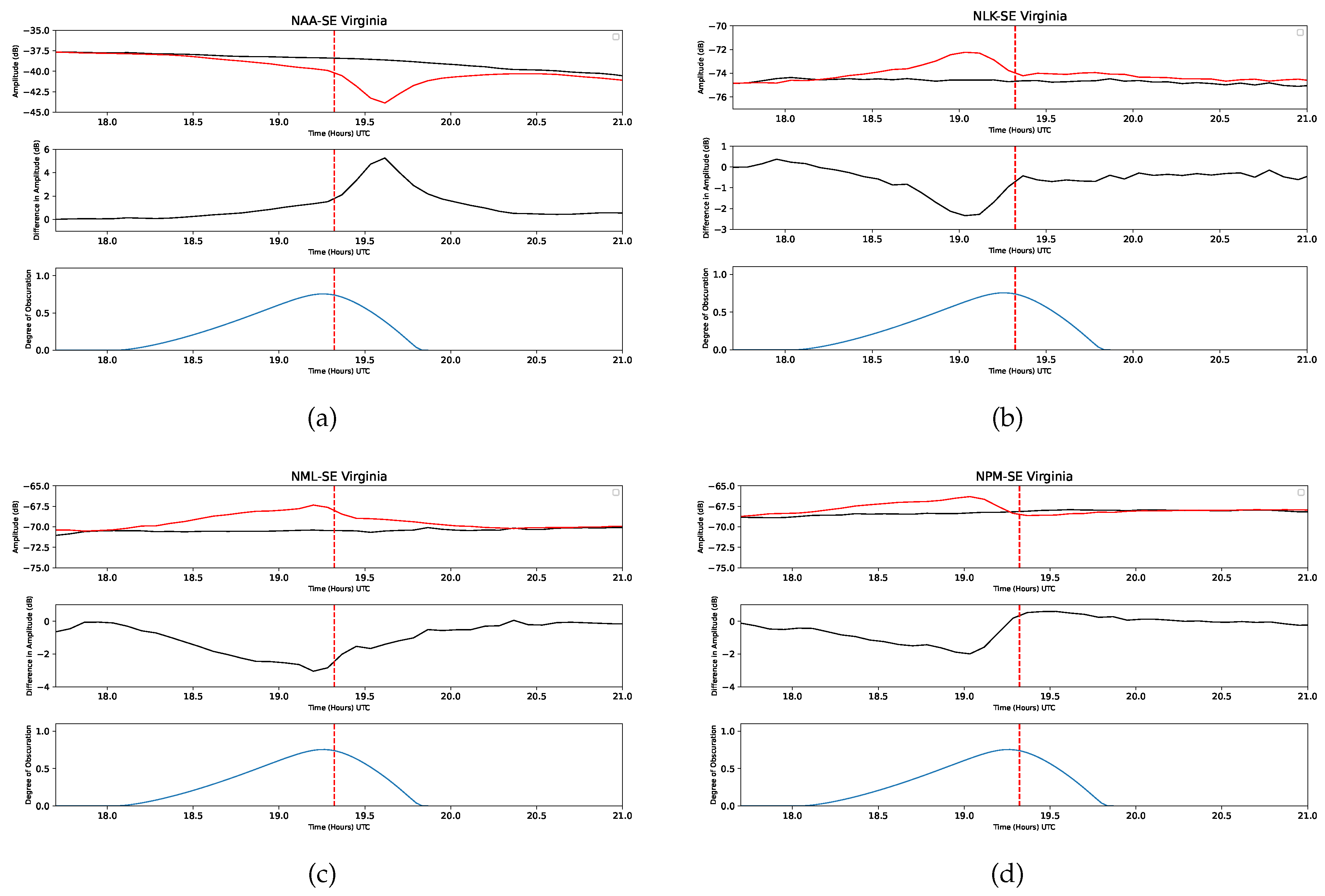
Figure 10.
VLF signal amplitude profiles during the eclipse and non-eclipse days observed from a VLF receiver located in Fife, Scotland, for the transmitter-receiver path (a) NAA-Fife and (b) NSY-Fife, plotted as a function of time (UTC) in hours. The upper row of each panel compares amplitude variations for the eclipse day (red curve) and a non-eclipse day (black curve), while the middle row illustrates the amplitude profile difference between the eclipse and non-eclipse days. Similarly, temporal variation of amplitude profiles during both eclipse and non-eclipse days observed from a VLF receiver located in Louargat, France, for the transmitter-receiver path (c) NAA-Louargat and (d) NSY-Louargat, plotted as a function of time (UTC) in hours. The red curve represents the eclipse day, and the black and green curves represent non-eclipse days.
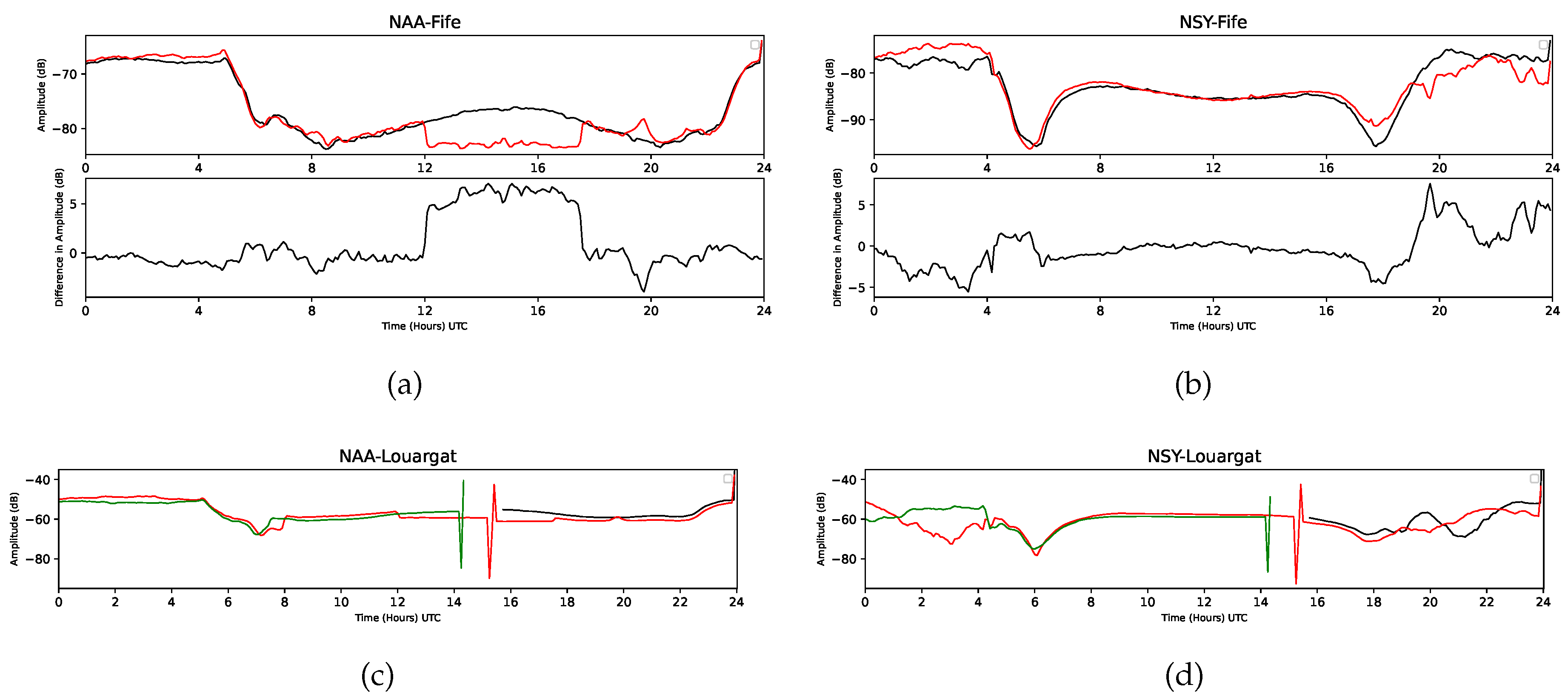
The VLF signal is transmitted from the NAA and NSY transmitters to a receiver located in Fife, Scotland, UK. This presents a unique situation where there was no eclipse at the receiver location, but the VLF signal path from the transmitter to the receiver experienced the eclipse. Consequently, the eclipse’s effect was observed on the VLF signal amplitude. The eclipse time is between 19:30 to 20:00 UTC for both NAA and NSY. The positive amplitude change was recorded for both cases, with 7.05 dB for the NAA-Fife path and 7.57 dB for the NSY-Fife path.
We have also recorded the VLF signal amplitude at Louargat, France, transmitted from the NAA and NSY transmitters. In this case, the receiver location did not experience any eclipse, but the effect on VLF amplitude was observed due to the VLF propagation path experiencing the eclipse. The eclipse time is between 19:30 to 20:31 UTC for both NAA and NSY. Since we do not have the full-day data for non-eclipse days in this case, we cannot determine the amplitude change between eclipse and non-eclipse days for the NAA-Louargat and NSY-Louargat paths.
In Figure 11a and Figure 11b, the corresponding phase change is presented for the transmitters NPM and NAA. The negative phase change was for NPM, and the positive phase change observed was for NAA. It is noted that the phase data for the stations NML and NLK were not appropriate for analysis (corrupted), so these are not presented.
Geomagnetic storms caused by solar activity are known to disrupt the ionosphere. We examine solar and geomagnetic data from April 5 to April 11, 2024 to assess if such a storm influenced the ionosphere during the eclipse. We obtain hourly measurements of Dst (storm intensity), Kp (planetary geomagnetic activity), Ap (auroral electrojet activity), solar flux (F10.7), Lyman-alpha radiation, and the northward component of the interplanetary magnetic field (IMF Bz) from the NASA OMNIWeb database (https://omniweb.gsfc.nasa.gov/). Figure 12 shows the observed temporal variations in these parameters (Dst, Kp, Ap etc.) indicating minimal solar and geomagnetic activity around the eclipse period (April 5 to April 11, 2024). This confirm that our measurements are not significantly affected by external disturbances, allowing us to attribute the observed ionospheric changes primarily to the solar eclipse.
4. Discussion
The manuscript examines the ionospheric response to the total solar eclipse on April 8, 2024, using both ground and space-based observations. The study is conducted under quiet geomagnetic conditions to avoid contamination. The modulation in the ionospheric vertical total electron content (VTEC) is analyzed to attribute ionospheric perturbations to the solar eclipse. The path of the eclipse (see Figure 1) spans a latitude range from N to S and a longitude range from W to E. Data from ten IGS stations, three VLF receiving stations, the GIM database, the DLR’s database, the Swarm satellite, and the COSMIC satellite is used to compute both quiet and perturbed VTEC profiles. The IGS and VLF stations are selected to experience the maximum solar eclipse under varying solar illumination and ionospheric conditions. For instance, some GNSS-IGS stations (NRC1, ACSO, STJO, HLFX) experience solar radiation blockage in the local afternoon, while SGPO experiences it at noon and INEG in the pre-noon period. Consequently, the VTEC profiles show varied perturbations, as illustrated in Figure 3. Similarly, among the UNAVCO-IGS stations, P776 and SA56 experience solar occultation in the local afternoon, P777 at noon, and TNCU in the pre-noon period. The VTEC variations exhibit a combined effect of regular solar flux changes and additional radiation blockage. Solar flux exhibits spatial and temporal variability across different geographic locations. Thus, changes in VTEC can be lower even with higher obscuration and vice versa. The pre-noon and post-noon effects of the eclipse are visible in the TEC profiles. Despite this variability, all stations consistently show a decrease in VTEC during the solar eclipse. profiles are modeled using data from the GIM and DLR’s databases to differentiate between quiet and eclipse-perturbed conditions. Our analysis reveals a depletion in proportional to the degree of solar obscuration observed by Swarm and COSMIC-2 satellites. This phenomenon arises from variations in chemical composition coupled with day-to-day fluctuations and differing production and recombination rates across altitudes.
The analysis of VLF signal amplitude profiles reveals significant variations during the solar eclipse, highlighting the effects of the eclipse on sub-ionospheric propagation paths. For paths received in rural SE Virginia, USA, positive amplitude changes were observed for NPM, NML, and NLK transmitters, with the maximum recorded at 0.5986 dB for NPM. In comparison, a negative change of 5.25 dB was noted for NAA. Unique effects were observed for VLF signals received in Fife, Scotland, where the receiver did not experience the eclipse. Still, the propagation paths from NAA and NSY did, leading to positive amplitude changes of 7.05 dB and 7.57 dB, respectively. Similarly, for signals received in Louargat, France, the receiver remained outside the eclipse path, yet propagation effects were evident due to the eclipse-affected paths. However, these paths’ lack of full-day non-eclipse data prevents a direct comparison. These observations underscore the complex interplay between VLF propagation characteristics and eclipse-induced ionospheric changes, varying by geographic location and path-specific factors.
This study stands out by focusing on the variation of the upper atmosphere during a total solar eclipse, leveraging a comprehensive range of space-based and ground-based networks worldwide. While many scientists have conducted similar research, they typically utilized a more limited set of tools. For instance, using data from six GNSS-IGS stations, [39] examined the VTEC profile changes during two different solar eclipses. Similarly, [34] investigated the VTEC profile variations during an annular eclipse with data from fifty-five GNSS-IGS stations and the Swarm Satellite, noting that most stations observed a decrease in the VTEC profile during solar occultation. Notably, the VTEC profile from Swarm Sat-A shows an almost 28% reduction on the eclipse day compared to the reference day. Our results corroborate previous research demonstrating a decrease in VTEC during solar eclipses [35,36,37,38].
Recently, [25] presented a multi-instrumental analysis of the same eclipse event, focusing on GNSS Vertical Electron Content (VEC), F-region irregularities using ionosonde measurements, and outcomes from SWARM satellite data. Their results for VTEC showed satisfactory agreement with our current study, corroborating many aspects of our findings. However, distinct differences between their data and outcomes are evident. In this manuscript, VTEC data from multiple sources, including IGS, UNAVCO, GIM, and SWE, are analyzed to examine depletion profiles. Our results reveal a similar depletion range of 15 to 5 TECU units, consistent with the findings reported by [25]. However, a few stations in our study, notably TNCE and INEG, did not exhibit significant changes. Furthermore, all ten IGS and UNAVCO stations in our analysis were selected from within the 90% lunar obscuration zone, differing from their methodology. To investigate the spatiotemporal profile, we utilized direct data from the GIM and SWE databases to extract changes in VTEC. Notably, differences were observed in the electron density profiles derived from SWARM data, likely due to variations in observation times. While our analysis focused on the interval between 08:51 UT and 09:03 UT, [25] reported their observations between 17:00 UT and 18:20 UT. Additionally, this manuscript extends the scope to include F-layer irregularities and examines the effects on the D-layer through sub-ionospheric VLF wave propagation. Despite employing different approaches, a comparative assessment shows that our results align well with those of [25], providing a complementary perspective on the studied eclipse event.
5. Conclusions
This study leverages the total solar eclipse of April 8, 2024, as a natural experiment to investigate the ionospheric response, focusing on the F-layer dynamics. The changes in Vertical Total Electron Content (VTEC) during a solar eclipse are primarily caused by the temporary reduction in solar radiation reaching the Earth’s atmosphere. Additionally, the cooling of the upper atmosphere during the eclipse reduces the recombination rate of electrons and ions. The reduction in temperature and the resulting changes in pressure gradients also influence atmospheric dynamics, such as the generation of atmospheric gravity waves, which further modulate ionospheric electron density. These combined effects produce a distinct depletion of VTEC, which varies based on the duration, path, and magnitude of the eclipse, as well as the local time and geographic location. By employing a comprehensive multi-instrument approach, which integrates data from ground-based GNSS and VLF stations, space-based observations from Swarm and COSMIC2 satellites, and spatiotemporal analyses using the Global Ionospheric Map (GIM) and DLR databases, we provide robust evidence of ionospheric variability during the eclipse. The results consistently reveal a significant depletion in the Total Electron Content (TEC) during the partial and total phases of the eclipse, correlating strongly with the degree of solar obscuration. This reduction in ionization is consistent with the established principle that decreased solar radiation leads to diminished ionospheric electron densities. Additionally, the VLF signal analysis shows fluctuations in amplitude and phase, complementing the GNSS-based TEC observations and highlighting the eclipse’s impact on ionospheric conductivity and wave propagation. Geomagnetic data confirm that external space weather disturbances did not influence the results, validating the isolation of eclipse-induced effects. This study’s findings enhance our understanding of ionospheric dynamics during solar eclipses and underscore the utility of multi-instrument campaigns for capturing spatiotemporal variability in the ionosphere.
This manuscript is significant in its comprehensive investigation of the ionospheric response to the total solar eclipse, as it integrates observations of both the lower and upper ionosphere using ground-based and space-based instruments. The study provides a multi-layered perspective on eclipse-induced ionospheric changes by leveraging VLF signal data to capture the lower ionospheric perturbations and satellite-derived VTEC profiles to analyze upper ionospheric dynamics. This dual approach allows for a detailed characterization of ionospheric processes, including variations in electron density, production and recombination rates, and propagation effects along eclipse-affected paths. Such an integrative methodology offers new insights into the coupling mechanisms between the ionosphere’s layers, enriching the understanding of solar-terrestrial interactions during eclipses. Future research will focus on integrating high-resolution models and extending observational networks to explore the coupling between ionospheric and thermospheric responses during eclipses, offering deeper insights into the interplay between solar radiation and upper atmospheric processes.
Author Contributions
“Conceptualization, S.S., A.D., and S.M.P; methodology, S.S. and A.D.; software, A.S., B.B., S.K.M., S.S.; validation, S.S., B.B., A.D., H.H., formal analysis, A.S., B.B., S.K.M, investigation, S.S., A.D., S.K.M., and H.H.; resources, J.M.P, P.N. J.B., S.J.; data curation, A.S., B.B., S.K.M., S.M.P, A.K.M, and S.S.; writing—original draft preparation, A.D., S.M.P. S.S.; >writing—review and editing, S.M.P., P.P., A.K.M, and S.R.; visualization, P.P., and S.R; supervision, A.D and S.S.; project administration, S.S.; funding acquisition, Y.Y.
Funding
This research received no external funding.
Data Availability Statement
The open-source data are available on their corresponding websites, as mentioned in the manuscript.
Acknowledgments
The authors acknowledge Dr. Gopi K. Seemala for providing the GPS-TEC software for the major computation. The authors also acknowledge the IGS, Swarm, COSMIC, GIM, SWE, and NASA Omniweb database team members for various data used in this article.
Conflicts of Interest
The authors declare no conflicts of interest.
Abbreviations
The following abbreviations are used in this manuscript:
| VTEC | Vertical Total Electron Content |
| STEC | Slant Total Electron Content |
| GIM | Global Ionospheric Map |
| IGS | International GNSS Service |
| GNSS | Global Navigational Satellite System |
| VLF | Very Low Frequency |
| UNAVCO | University NAVSTAR Consortium |
References
- Bracewell, R. N. Theory of formation of an ionospheric layer below E layer based on eclipse and solar flare effects at 16 kc/sec. Journal of Atmospheric and Terrestrial Physics 1952, 2, 226–235. [Google Scholar] [CrossRef]
- Crary, J. H.; Schneible, D. E. Effect of the eclipse of 20 July 1963 on VLF signals propagating over short paths. Radio Science 1965, 69D, 947–957. [Google Scholar] [CrossRef]
- Sen Gupta, A.; Goel, G. K.; Mathur, B. S. Effect of the 16 February 1980 solar eclipse on VLF propagation. Journal of Atmospheric and Terrestrial Physics 1980, 42, 907–909. [Google Scholar] [CrossRef]
- Clilverd, M. A.; Rodger, C. J.; Thomson, N. R.; Lichtenberger, J.; Steinbach, P.; Cannon, P.; Angling, M. J. Total solar eclipse effects on VLF signals: Observations and modeling. Radio Science 2001, 36, 773–788. [Google Scholar] [CrossRef]
- Chakrabarti, S. K.; Sasmal, S.; Pal, S.; Mondal, S. K. Results of VLF campaigns in summer, winter and during solar eclipse in Indian subcontinent and beyond. AIP Conference Proceedings 2010, 1286, 61–76. [Google Scholar] [CrossRef]
- Pal, S.; Chakrabarti, S. K.; Mondal, S. K. Modeling of sub-ionospheric VLF signal perturbations associated with total solar eclipse, 2009 in Indian subcontinent. Advances in Space Research 2012, 50, 196–204. [Google Scholar] [CrossRef]
- Chakraborty, S.; Palit, S.; Ray, S.; Chakrabarti, S. K. Modeling of the lower ionospheric response and VLF signal modulation during a total solar eclipse using ionospheric chemistry and LWPC. Astrophysics and Space Science 2016, 361, 1–15. [Google Scholar] [CrossRef]
- Chakraborty, S.; Chakrabarti, S. K.; Palit, S.; Ray, S. Modeling of the lower ionospheric response and VLF signal modulation during a total solar eclipse using ionospheric chemistry and LWPC. 42nd COSPAR Scientific Assembly 2018, 42, C0-3. [Google Scholar] [CrossRef]
- Möllmann, K. P.; Vollmer, M. Measurements and predictions of the illuminance during a solar eclipse. European Journal of Physics 2006, 27, 1299. [Google Scholar] [CrossRef]
- Cheng, W.; Xu, W.; Gu, X.; Wang, S.; Wang, Q.; Ni, B.; Lu, Z.; Xiao, B.; Meng, X. A comparative study of VLF transmitter signal measurements and simulations during two solar eclipse events. Remote Sensing 2023, 15, 3025. [Google Scholar] [CrossRef]
- Ercha, A.; Zhang, S. R.; Erickson, P. J.; Goncharenko, L. P.; Coster, A. J.; Jonah, O. F.; Lei, J.; Huang, F.; Dang, T.; Lei, L. Coordinated ground-based and space-borne observations of ionospheric response to the annular solar eclipse on 26 December 2019. Journal of Geophysical Research: Space Physics 2020, 125. [Google Scholar] [CrossRef]
- Kumar, S.; Kumar, A.; Maurya, A. K.; Singh, R. Changes in the D region associated with three recent solar eclipses in the South Pacific region. Journal of Geophysical Research: Space Physics 2016, 121, 5930–5943. [Google Scholar] [CrossRef]
- Mitra, A. P. Ionospheric effects of solar flares. Astrophysics and Space Science Library 1974, 46. [Google Scholar] [CrossRef]
- Bagiya, M.; Joshi, H.; Iyer, K.; Aggarwal, M.; Ravindran, S.; Pathan, B. M. TEC variations during low solar activity period (2005–2007) near the Equatorial Ionospheric Anomaly Crest region in India. Annales Geophysicae 2009, 27. [Google Scholar] [CrossRef]
- Hussien, F.; Ghamry, E.; Fathy, A.; Mahrous, S. Swarm Satellite Observations of the 21 August 2017 Solar Eclipse. Journal of Astronomy and Space Sciences 2020, 37, 29–34. [Google Scholar] [CrossRef]
- Fathy, A.; Ghamry, E.; Arora, K. Mid and low-latitudinal ionospheric field-aligned currents derived from the Swarm satellite constellation and their variations with local time, longitude, and season. Advances in Space Research 2019, 64, 1600–1614. [Google Scholar] [CrossRef]
- Friis Christensen, E.; Lühr, H.; Hulot, G. Swarm: A constellation to study the Earth’s magnetic field. Earth, Planets and Space 2006, 58, 351–358. [Google Scholar] [CrossRef]
- Friis-Christensen, E.; Lühr, H.K.D.; Haagmans, R. Swarm - an Earth observation mission investigating geospace. Advances in Space Research 2008, 41, 210–216. [Google Scholar] [CrossRef]
- Kundu, S.; Sasmal, S.; Chakrabarti, S. K. Long-term ionospheric VTEC variation during solar cycle 24 as observed from Indian IGS GPS station. International Journal of Scientific Research in Physics and Applied Sciences 2021, 9. [Google Scholar] [CrossRef]
- Kundu, S.; Chowdhury, S.; Palit, S.; Mondal, S. K.; Sasmal, S. Variation of ionospheric plasma density during the annular solar eclipse on December 26, 2019. Astrophysics and Space Science 2022, 367, 44. [Google Scholar] [CrossRef]
- Rama Rao, P. V. S.; Gopi K., S.; Niranjan, K.; Prasad, D. S. V. V. D. Temporal and spatial variations in TEC using simultaneous measurements from the Indian GPS network of receivers during the low solar activity period of 2004–2005. Annales Geophysicae 2006, 24, 3279–3292. [Google Scholar] [CrossRef]
- Seemala, G.; Valladares, C. Statistics of total electron content depletions observed over the South American continent for the year 2008. Radio Science 2011, 46, 1–14. [Google Scholar] [CrossRef]
- Rao, P.; Seemala, G.; Niranjan, K.; Prasad, D. Study of spatial and temporal characteristics of L-band scintillations over the Indian low-latitude region and their possible effects on GPS navigation. Annales Geophysicae 2006, 24. [Google Scholar] [CrossRef]
- Olsen, N.; Friis-Christensen, E.; Floberghagen, R.; Alken, P.; Beggan, C. D.; Chulliat, A.; Doornbos, E.; Da Encarnação, J. T.; Hamilton, B.; Hulot, G.; et al. The Swarm satellite constellation application and research facility (SCARF) and Swarm data products. Earth, Planets and Space 2013, 65, 1189–1200. [Google Scholar] [CrossRef]
- Zhang, H.; Zhang, T.; Zhang, X.; Yuan, Y.; Wang, Y.; Ma, Y. Multi-Instrument Observations of the Ionospheric Response Caused by the 8 April 2024 Total Solar Eclipse. Remote Sens 2024, 16, 2451–10.3390. [Google Scholar] [CrossRef]
- Rama Rao, P. V. S.; Niranjan, K.; Prasad, D. S. V. V. D.; Gopi Krishna, S.; Uma, G. On the validity of the ionospheric pierce point (IPP) altitude of 350 km in the Indian equatorial and low-latitude sector. Annales Geophysicae 2006, 24, 2159–2168. [Google Scholar] [CrossRef]
- Klobuchar, J. A. Design and characteristics of the GPS ionospheric time delay algorithm for single frequency users. PLANS’86-Position Location and Navigation Symposium 1986, 280–286. [Google Scholar] [CrossRef]
- Eyelade, V. A.; Adewale, A. O.; Akala, A. O.; Bolaji, O. S.; Rabiu, A. B. Studying the variability in the diurnal and seasonal variations in GPS total electron content over Nigeria. Annales Geophysicae 2017, 35, 701–710. [Google Scholar] [CrossRef]
- Marković, M. Determination of total electron content in the ionosphere using GPS technology. Geonauka 2014, 2, 1–9. [Google Scholar] [CrossRef]
- Hoque, M. M.; Jakowski, N.; Prol, F. S. A new climatological electron density model for supporting space weather services. Journal of Space Weather and Space Climate 2022, 12. [Google Scholar] [CrossRef]
- Herring, T. A.; Melbourne, T. I.; Murray, M. H.; Floyd, M. A.; Szeliga, W. M.; King, R. W.; Phillips, D. A.; Puskas, C. M.; Santillan, M.; Wang, L. Plate Boundary Observatory and related networks: GPS data analysis methods and geodetic products. Reviews of Geophysics 2016, 54, 759–808. [Google Scholar] [CrossRef]
- Zhang, R.; Le, H.; Li, W.; Ma, H.; Yang, Y.; Huang, H.; Li, Q.; Zhao, X.; Xie, H.; Sun, W.; et al. Multiple technique observations of the ionospheric responses to the 21 June 2020 solar eclipse. Journal of Geophysical Research: Space Physics 2020, 125, e2020JA028450. [Google Scholar] [CrossRef]
- Jakowski, N.; Mayer, C.; Hoque, M. M.; Wilken, V. Total electron content models and their use in ionosphere monitoring. Radio Science 2011, 46, 1–11. [Google Scholar] [CrossRef]
- Das, S.; Maity, S. K.; Nanda, K.; Jana, S.; Brawar, B.; Panchadhyayee, P.; Datta, A.; Sasmal, S. Study of the response of the upper atmosphere during the annular solar eclipse on October 14, 2023. Advances in Space Research 2024, 74, 3344–3360. [Google Scholar] [CrossRef]
- Vyas, B. M.; Sunda, s. The solar eclipse and its associated ionospheric TEC variations over Indian stations on January 15, 2010. 2011, 49, 546–555. [Google Scholar] [CrossRef]
- Kumar, S.; Priyadarshi, S.; Gopi Krishna, S.; Singh, A. K. GPS-TEC variations during low solar activity period (2007–2009) at Indian low latitude stations. Astrophysics and Space Science 2012, 339, 165–178. [Google Scholar] [CrossRef]
- Hoque, M. M.; Wenzel, D.; Jakowski, N.; Gerzen, T.; Berdermann, J.; Wilken, V.; Minkwitz, D. Ionospheric response over Europe during the solar eclipse of March 20, 2015. Journal of Space Weather and Space Climate 2016, 6, A36. [Google Scholar] [CrossRef]
- Senapati, B.; Huba, J. D.; Kundu, B.; Gahalaut, V. K.; Panda, D.; Mondal, S. K.; Catherine, J. K. Change in total electron content during the 26 December 2019 solar eclipse: Constraints from GNSS observations and comparison with SAMI3 model results. Journal of Geophysical Research: Space Physics 2020, 125, e2020JA028230. [Google Scholar] [CrossRef]
- Valdés-Abreu, J. C.; Díaz, M.; Bravo, M.; Stable-Sánchez, Y. Ionospheric Total Electron Content Changes during the 15 February 2018 and 30 April 2022 Solar Eclipses over South America and Antarctica. Remote Sensing 2023, 15, 4810. [Google Scholar] [CrossRef]
Figure 1.
(top) The map illustrates the locations of the GNSS-IGS (yellow diamond) and UNAVCO-IGS (orange circle) stations with the totality belt of the solar eclipse. The red curve depicts the central track of totality. The upper and lower bounds of the total eclipse, represented by the blue dashed curves, indicate the regions where a total eclipse was observed. Outside these dashed curves, only a partial eclipse was visible. (bottom) Similar map with VLF transmitters with four VLF transmitters (red circles), three receiving locations (blue diamonds) and the great circle path between thems.
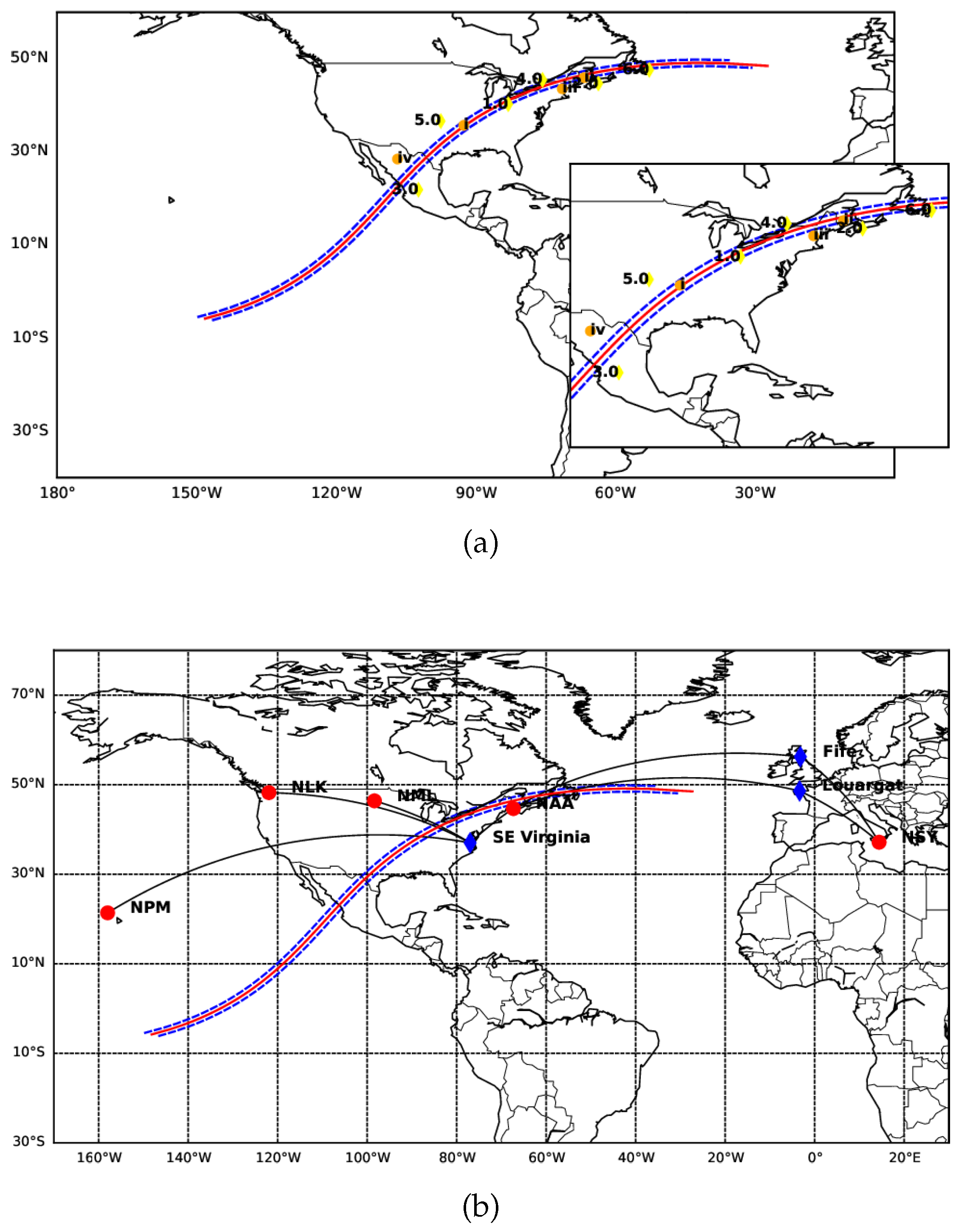
Figure 2.
(a) Geometric representation of the Sun and the Moon during a solar eclipse [9]. (b-d) The luminance and lunar shadow shadow at (a) start, (b) mid and (c) end of the eclipse over the totality belt.
Figure 2.
(a) Geometric representation of the Sun and the Moon during a solar eclipse [9]. (b-d) The luminance and lunar shadow shadow at (a) start, (b) mid and (c) end of the eclipse over the totality belt.
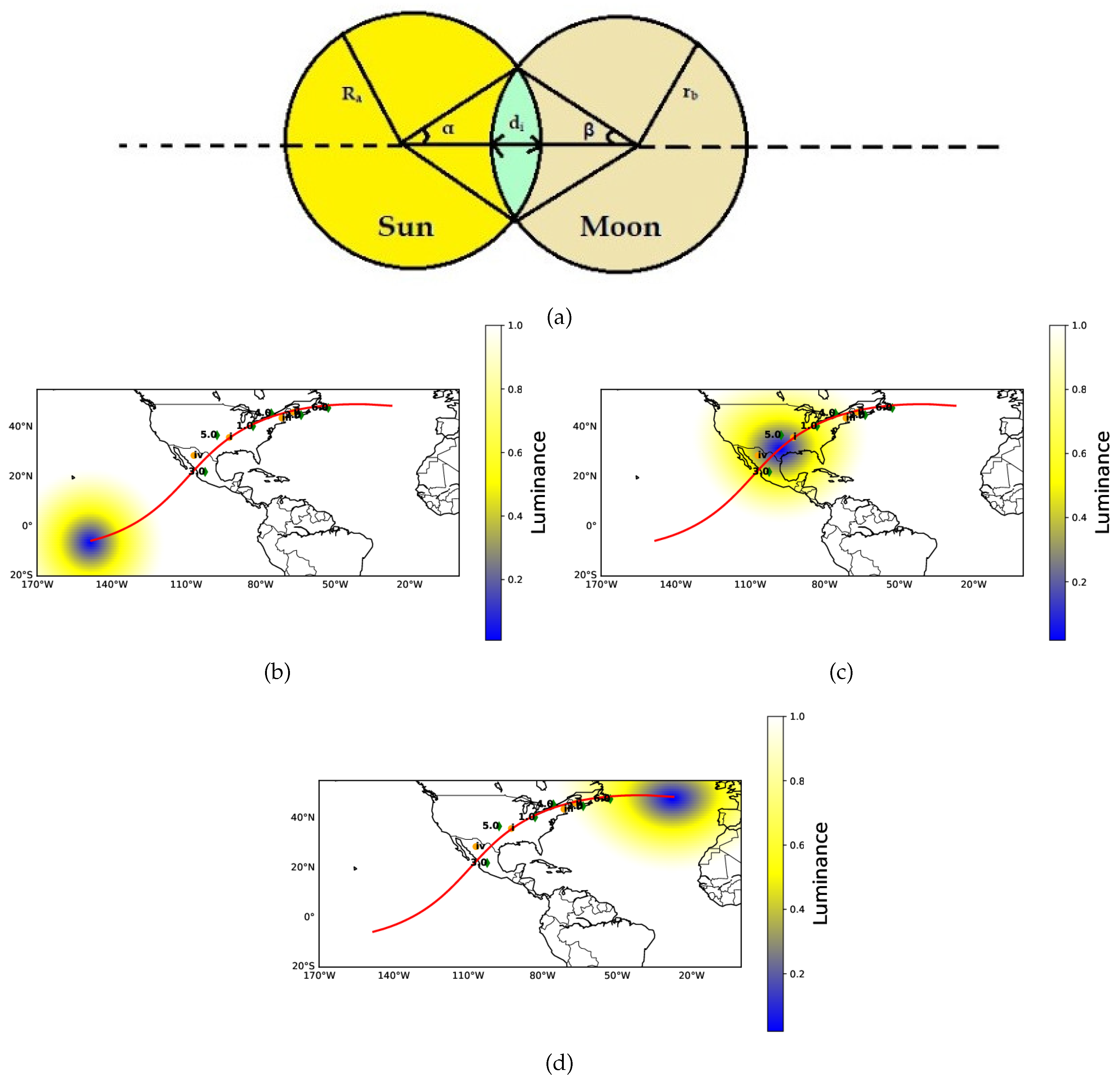
Figure 3.
Temporal variation of the profile as a function of time (UTC) in hours during the solar eclipse as observed from different GNSS-IGS stations. The upper panel of each profile illustrates the variation for three consecutive days: the day before the eclipse (black curve), the day of the eclipse (red curve), and the day after the eclipse (green curve). The middle panel shows the mean variations of the two non-eclipse days (black dashed curve) compared to the eclipse day (red curve). The lower panel indicates the degree of obscuration on the eclipse day.
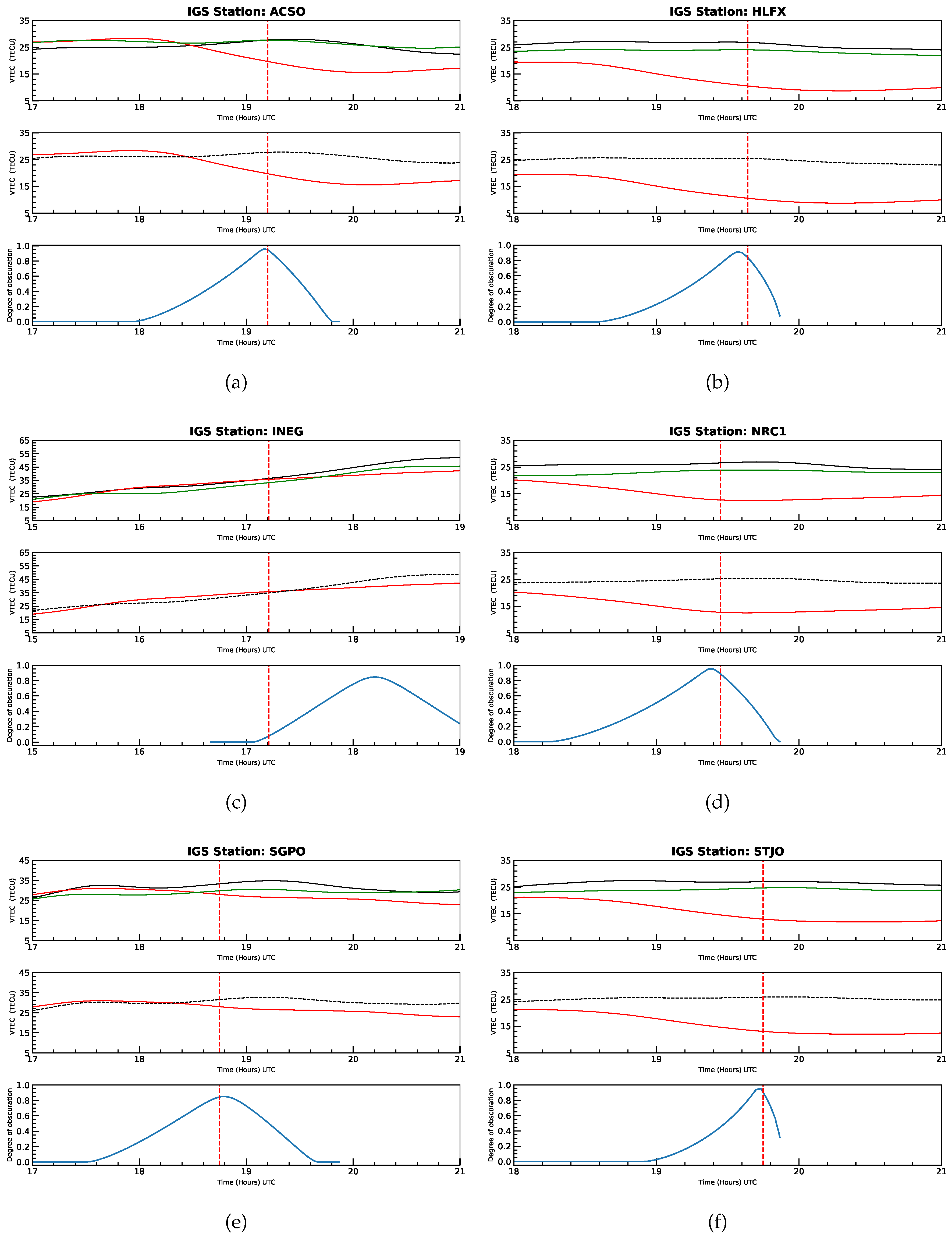
Figure 4.
Temporal variation of the profile as a function of time (UTC) in hours during the solar eclipse for the UNAVCO-IGS stations. The figure format and color codes are consistent with those in Figure 3.
Figure 4.
Temporal variation of the profile as a function of time (UTC) in hours during the solar eclipse for the UNAVCO-IGS stations. The figure format and color codes are consistent with those in Figure 3.
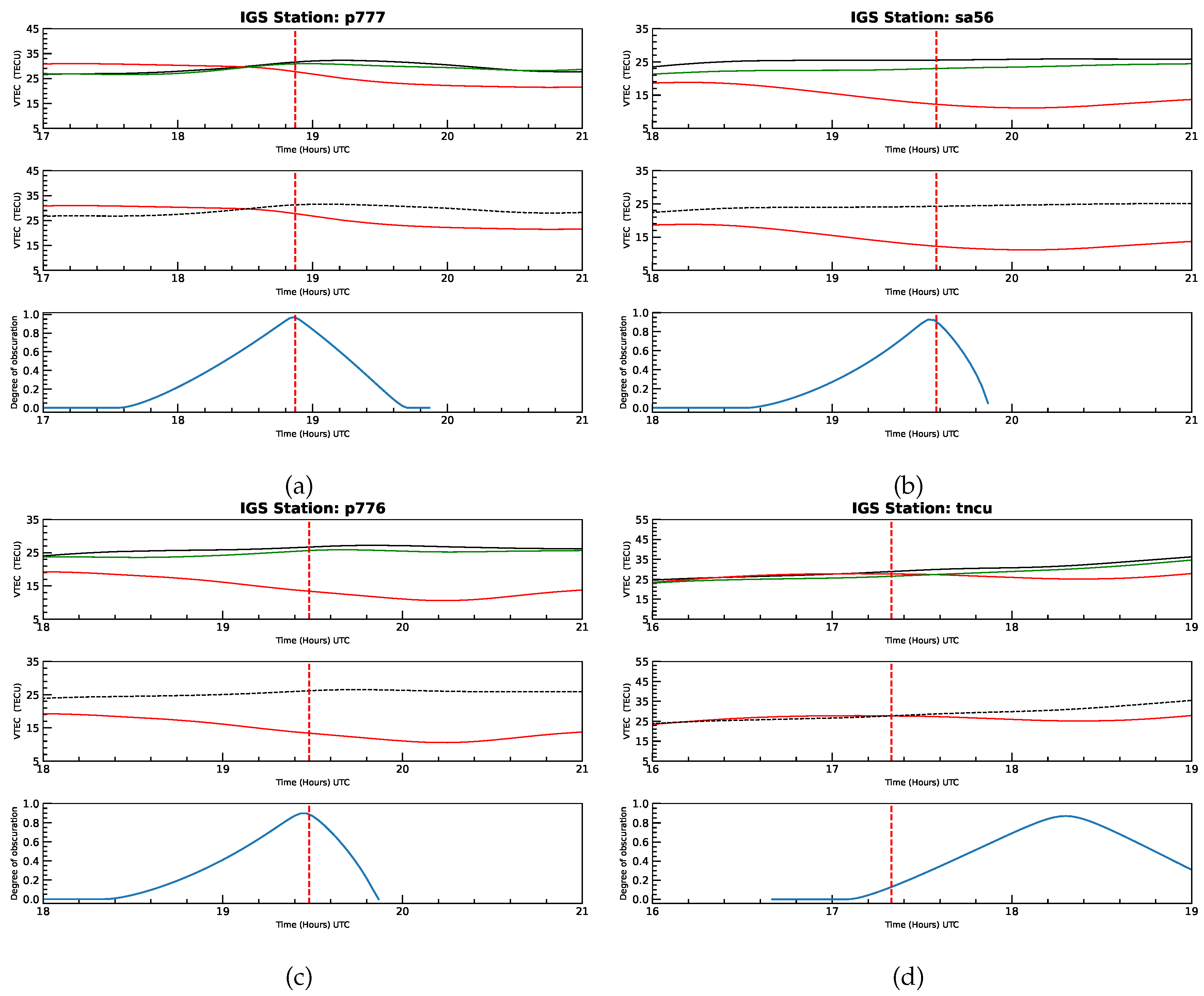
Figure 5.
(a) The temporal variation of profiles as a function of latitude as observed from the Swarm satellite. The upper panel shows the profiles for the eclipse day (red curve) and the non-eclipse day (black curve). The middle panel illustrates the difference in profiles between the eclipse day and the non-eclipse day. The lower panel presents the percentage difference in profiles. (b) The spatiotemporal variation of along the trajectory of Swarm-B satellite. (c) The temporal variation of average as a function of latitude as observed from the Swarm satellite. The figure format and color codes are the same as in Figure 5a. (d) The spatiotemporal profile is shown over the satellite track of the Swarm satellite for the eclipse and non-eclipse days.
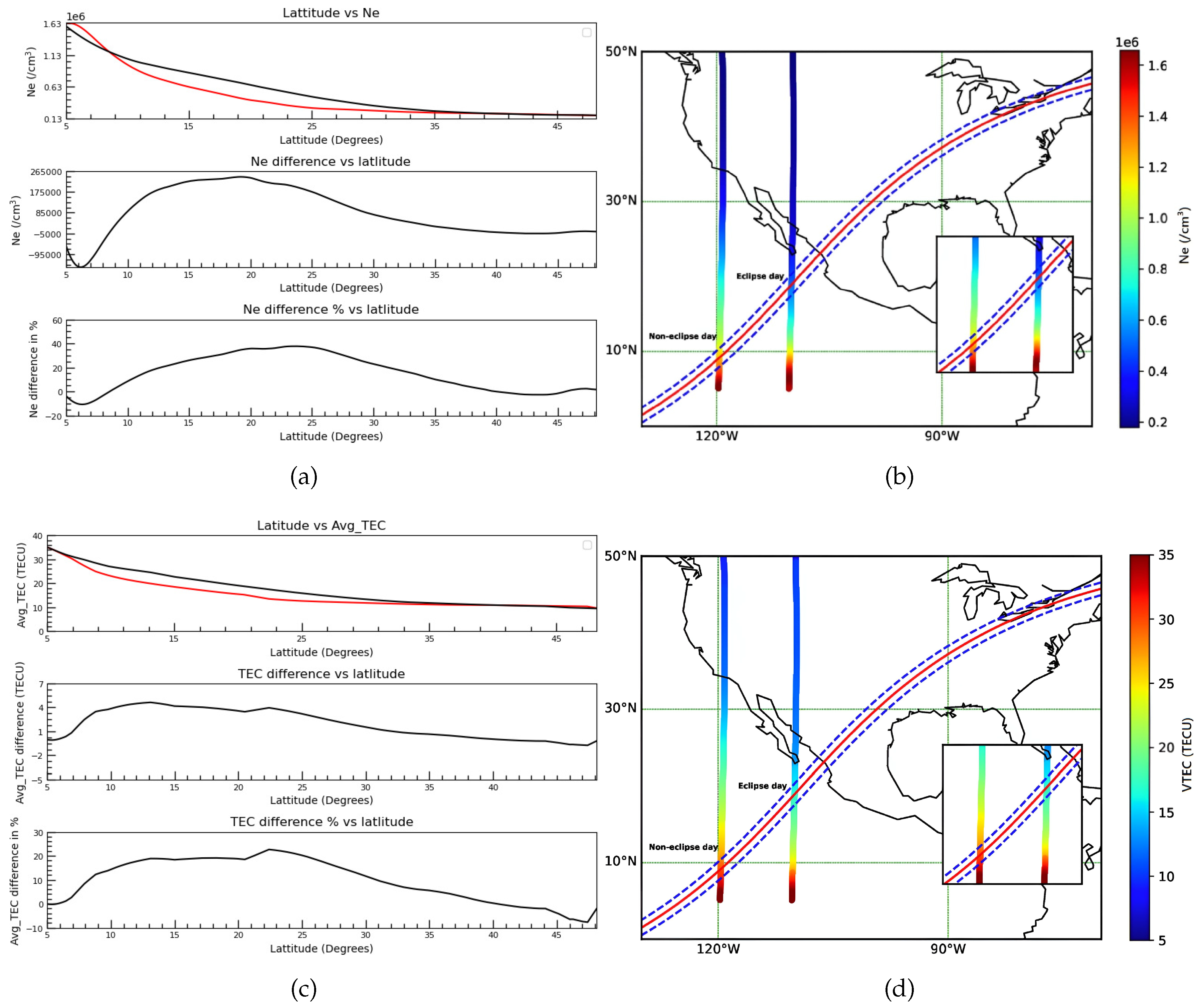
Figure 6.
(a) profiles during eclipse and non-eclipse days observed from the COSMIC-2 satellite constellation. The upper panel of each profile illustrates the variation of across a range of latitudes and longitudes, depicting data for eclipse (red curve) and non-eclipse days (black curve). The middle panel displays the difference in values (measured in ) between non-eclipse and eclipse days. The lower panel depicts the percentage change in the profile between eclipse and non-eclipse days. (b) The spatiotemporal profile is shown over the Cosmic satellite track for the eclipse and non-eclipse days.
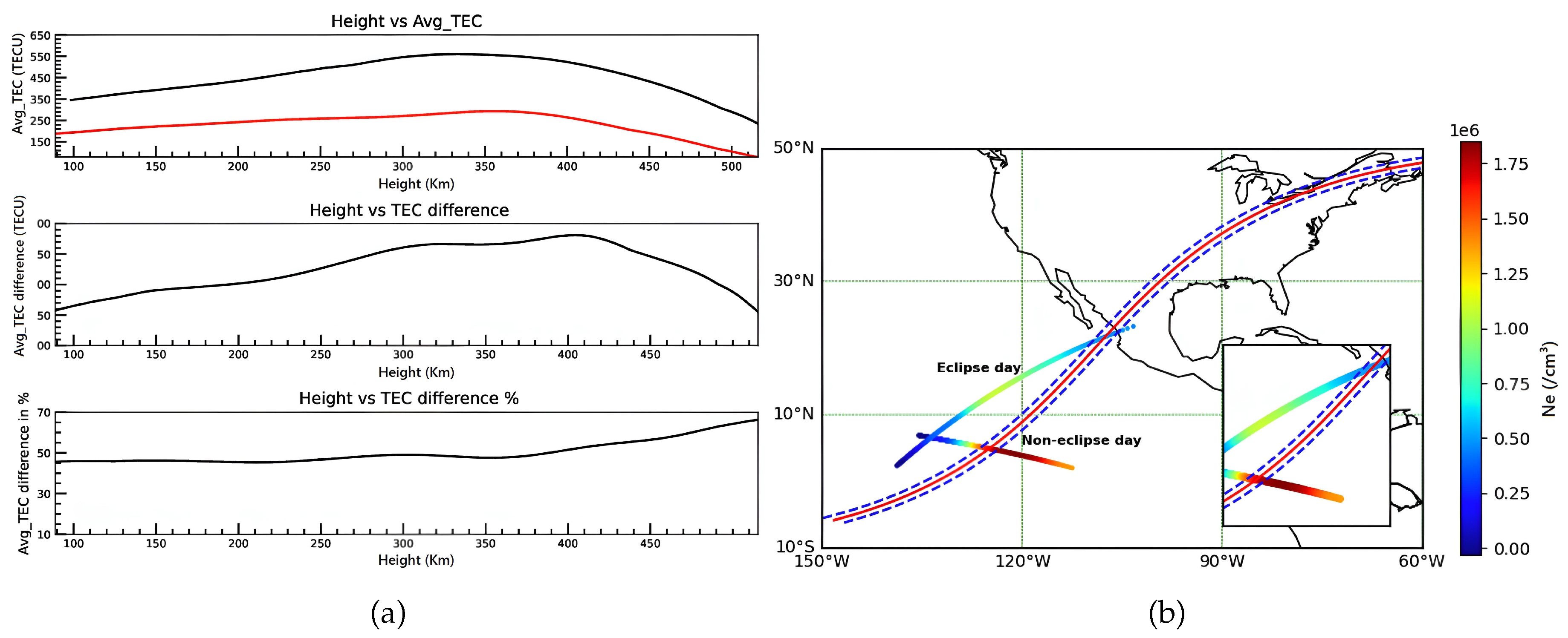
Figure 7.
Spatiotemporal profile of from 15:00 to 20:00 UTC as observed from GIM data for April 7 (top), 8 (middle), and 9 (bottom), 2024.
Figure 7.
Spatiotemporal profile of from 15:00 to 20:00 UTC as observed from GIM data for April 7 (top), 8 (middle), and 9 (bottom), 2024.
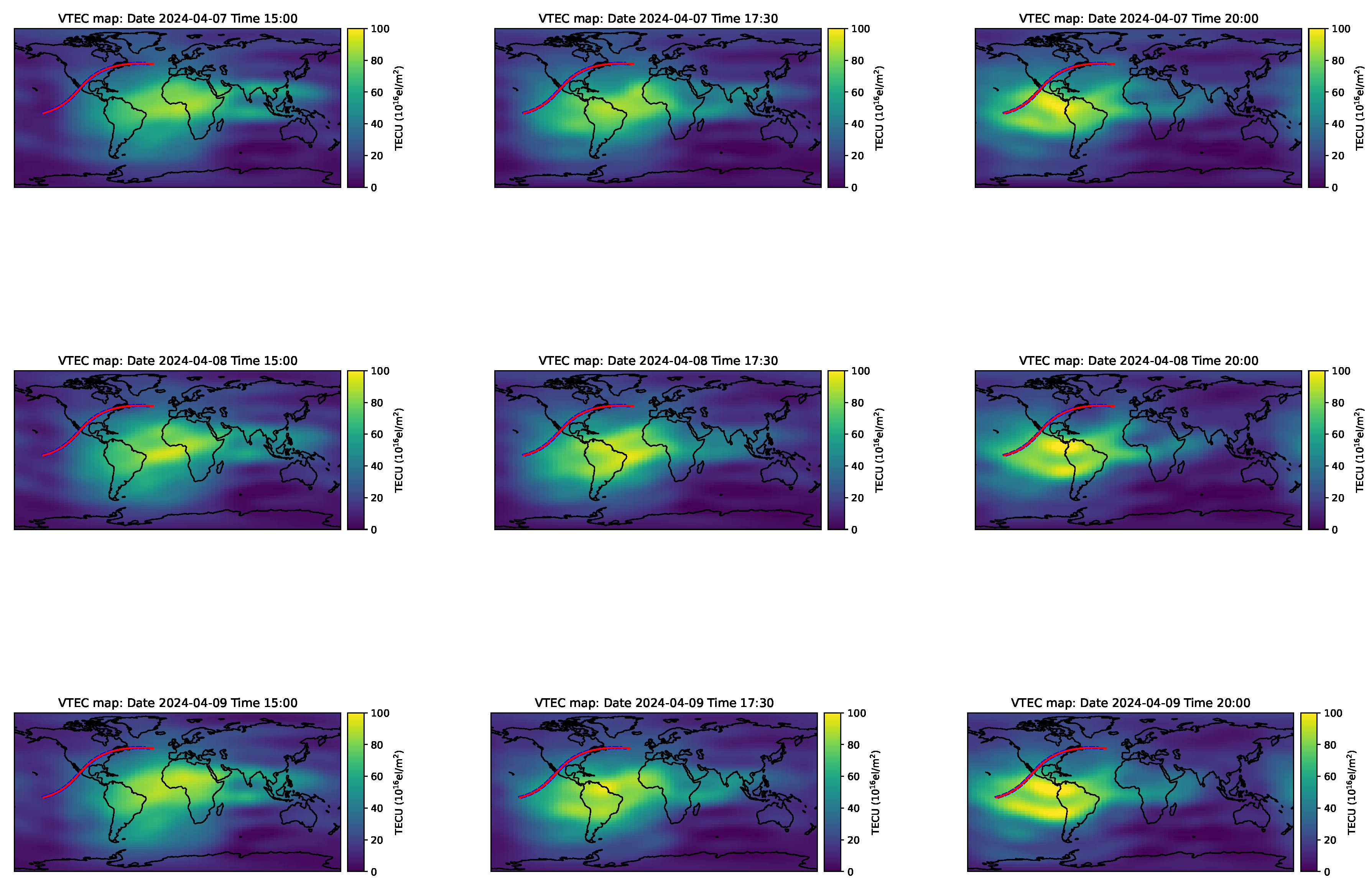
Figure 8.
Spatiotemporal profile of from 15:00 to 20:00 UTC as observed from SWE data for April 7 (top), 8 (middle), and 9 (bottom), 2024.
Figure 8.
Spatiotemporal profile of from 15:00 to 20:00 UTC as observed from SWE data for April 7 (top), 8 (middle), and 9 (bottom), 2024.
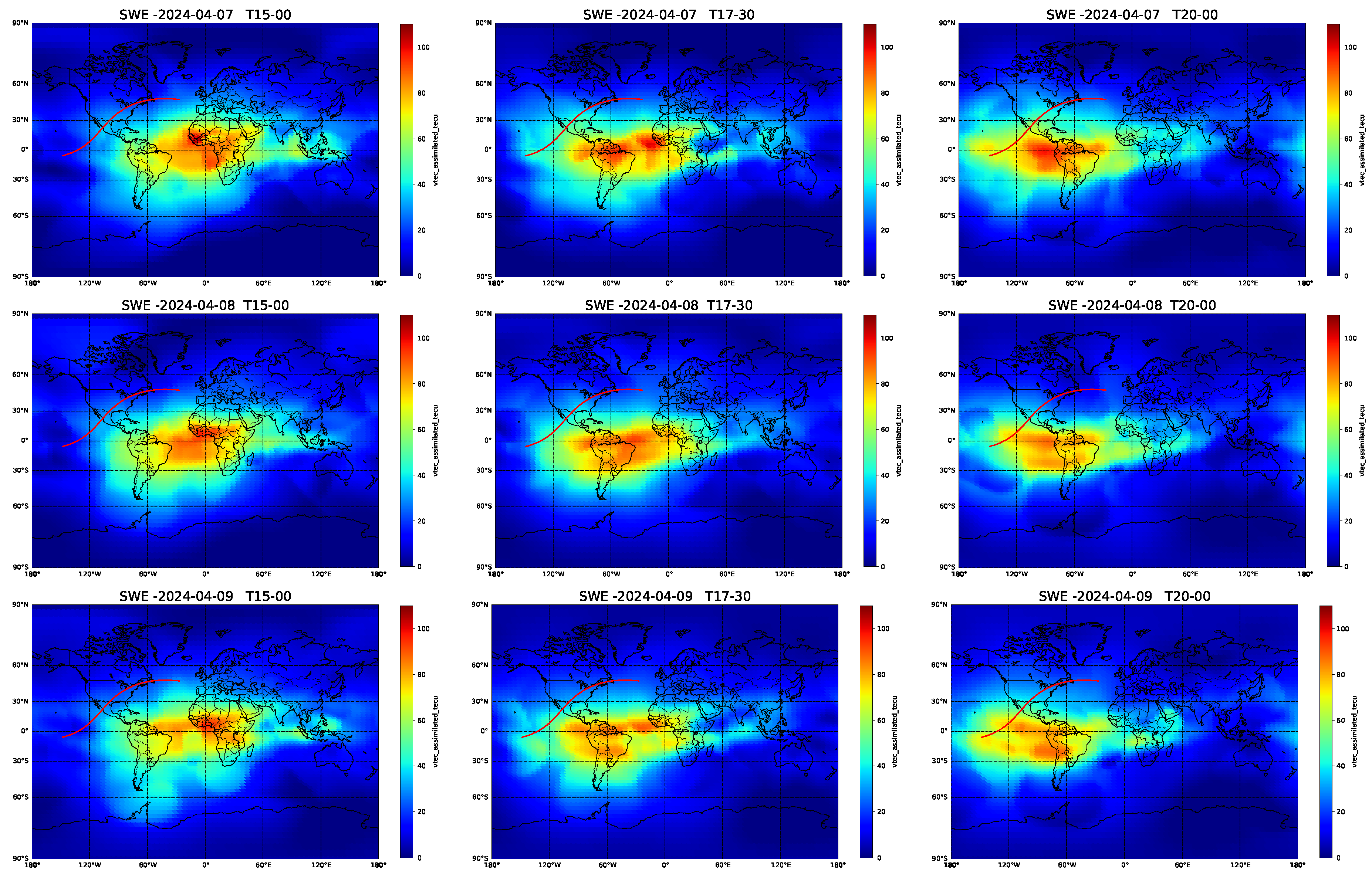
Figure 11.
Temporal variation of phase profiles during both eclipse and non-eclipse days as a function of time (UTC) in hours as observed from a VLF receiver located in rural SE Virginia, USA, for the transmitters (a) NAA, (b) NPM. The figure format and color codes per panel are the same as in Figure 9.
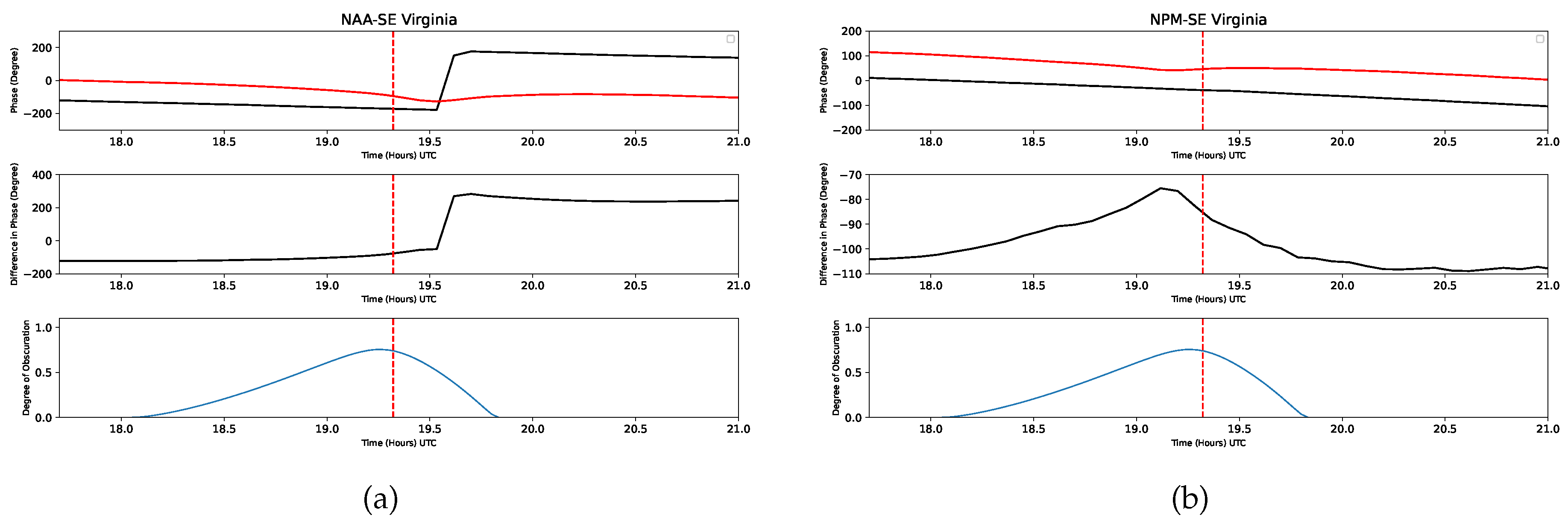
Figure 12.
Temporal variation of Dst, Ap, Kp, Solar Flux (F10.7), Lyman alpha, and IMF Bz for the time period 05-11 April, 2024. The red parts of the curves and histograms depict the variation specifically for the eclipse day.
Figure 12.
Temporal variation of Dst, Ap, Kp, Solar Flux (F10.7), Lyman alpha, and IMF Bz for the time period 05-11 April, 2024. The red parts of the curves and histograms depict the variation specifically for the eclipse day.
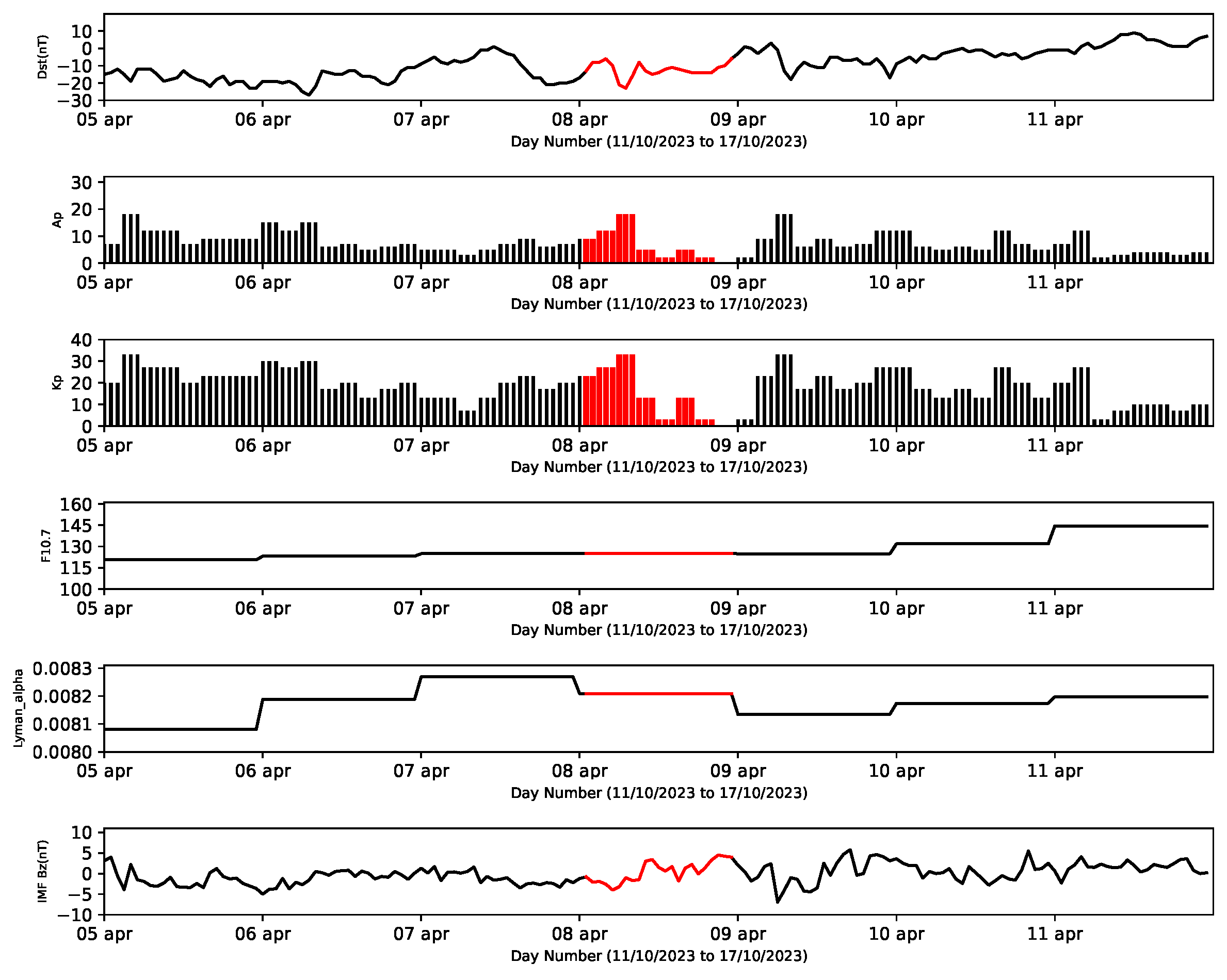

Table 1.
List of GNSS-IGS Stations
| Station Code | Region | Lat./Long. | Maximum Obsc.(%) | Max Depletion in TEC (%) |
|---|---|---|---|---|
| (I) NRC1 | Canada | N/ W | 100 | 50.92 |
| (II) ACSO | US | N/ W | 99.87 | 40.31 |
| (III) STJO | Canada | N/ W | 99.24 | 52.95 |
| (IV) HLFX | Canada | N/ W | 94.29 | 63.56 |
| (V) SGPO | US | N/ W | 93.64 | 26.06 |
| (VI) INEG | Mexico | N/ W | 90.67 | 18.09 |
Table 2.
List of UNAVCO-IGS Stations
| Station Code (Sl. No.) | Region | Lat./Long. | Maximum Obsc.(%) | Max Depletion in TEC (%) |
|---|---|---|---|---|
| (I) P777 | USA | N/ W | 100 | 25.25 |
| (II) SA56 | Canada | N/ W | 98.52 | 54.84 |
| (III) P776 | USA | N/ W | 92.59 | 59.36 |
| (IV) TNCU | Mexico | N/ W | 90.94 | 22.37 |
Disclaimer/Publisher’s Note: The statements, opinions and data contained in all publications are solely those of the individual author(s) and contributor(s) and not of MDPI and/or the editor(s). MDPI and/or the editor(s) disclaim responsibility for any injury to people or property resulting from any ideas, methods, instructions or products referred to in the content. |
© 2024 by the authors. Licensee MDPI, Basel, Switzerland. This article is an open access article distributed under the terms and conditions of the Creative Commons Attribution (CC BY) license (http://creativecommons.org/licenses/by/4.0/).
Copyright: This open access article is published under a Creative Commons CC BY 4.0 license, which permit the free download, distribution, and reuse, provided that the author and preprint are cited in any reuse.


