
Submitted:
29 April 2025
Posted:
29 April 2025
You are already at the latest version
Abstract
This study investigates the performance of three different signal combinations (L1-L2, L1-L5, and L2-L5) for estimating ionospheric Total Electron Content (TEC) and rate of TEC (ROT) using Quasi-Zenith Satellite System (QZSS) observations over the Korean Peninsula. GNSS data collected from nine stations across the Korean Peninsula were analyzed for the period from Day of Year (DOY) 1 to 182 in 2024. Differential Code Biases (DCBs) were estimated for QZSS satellites using a regional ionospheric model, showing high temporal stability. TEC values derived from different signal combinations were compared with the CODE Global Ionospheric Map (GIM). The L1-L5 combination yields the closest agreement with the CODE GIM in terms of both bias and root mean square (RMS) error. In addition, the ROT analysis over the consecutive six days revealed that the L1-L5 combination consistently exhibited the lowest RMS values. As a result, we suggest that the L1-L5 combination can provide better performance for QZSS-based ionospheric monitoring and TEC studies.
Keywords:
QZSS
; TEC
; ROT
; DCBs
1. Introduction
The Global Navigation Satellite System (GNSS) has proven to be a highly effective tool for estimating and continuously monitoring the total electron content (TEC) in the Earth’s ionosphere. TEC can be calculated with high precision from global or regional networks of GNSS reference stations [1,2,3]. Currently, modern GNSS constellations, such as the United States’ Global Positioning System (GPS), Russia’s GLObal NAvigation Satellite System (GLONASS), China’s BeiDou Navigation Satellite System (BDS), the European Union’s Galileo, India’s Navigation with Indian Constellation (NavIC), and Japan’s Quasi-Zenith Satellite System (QZSS), are capable of transmitting signals on dual or triple frequencies, which enhances positioning and ionospheric correction. While signals are functionally similar with different GNSS systems, they may differ in their center frequencies.
The GPS dual-frequencies, L1 (1575.42 MHz) and L2 (1227.60 MHz), have been predominantly used for accurate ionospheric TEC estimation [4,5]. With the increasing availability of ground-based GNSS receivers capable of tracking BDS and Galileo signals, the integration of multi-GNSS constellations has enabled more precise and reliable estimations of ionospheric TEC. Hu et al. [6] employed data collected from 30 GNSS reference stations distributed across China to estimate TEC based on BDS GEO satellite signals. Their results demonstrated that TEC derived from BDS GEO satellites can deliver continuous and reliable ionospheric observations even during storm conditions.
Satellites in Medium Earth Orbit (MEO), such as those comprising the GPS constellation, ensure extensive spatial coverage, while those in Geosynchronous Earth Orbit (GEO) and Inclined Geosynchronous Satellite Orbit (IGSO) enable sustained observation over specific locations or constrained regional areas [7]. Moreover, Yang et al. [8] showed that newer BDS signals, specifically B1C (1575.42 MHz) and B2a (1176.45 MHz), provide enhanced precision for ionospheric studies compared to the legacy B1I and B3I signals. Similarly, the Galileo system transmits signals at E1 (1575.42 MHz), E5a (1176.45 MHz), and E5b (1207.140 MHz), with the E1-E5a pair commonly used for ionospheric applications.
The QZSS is a Japanese regional navigation satellite system composed of three IGSO satellites and one GEO satellite. With the launch of three additional satellites, the system is scheduled to reach Full Operational Capability (FOC) by 2025 [9]. Despite the growing availability of GNSS stations capable of receiving multi-GNSS signals, those equipped to track QZSS signals remain predominantly concentrated in the East Asia and Oceania regions, reflecting the system’s regional operational design. Therefore, the sparse spatial distribution of QZSS-tracking stations constrains the feasibility of simultaneous modeling of ionospheric TEC and Differential Code Biases (DCBs) [10]. As a result, studies employing QZSS observations for TEC estimation remain limited.
A recent study [11] reported significant findings on ionospheric behavior based on QZSS observations, analyzing the ionospheric disturbances induced by the Fukutoku-Okanoba volcano using QZSS data collected in Japan. In addition, Choi et al. [12] estimated ionospheric TEC over the Korean Peninsula using QZSS L1 and L2 signals, reporting a high level of consistency with the TEC values derived by the Global Ionosphere Map (GIM) from the Center for Orbit Determination Europe (CODE).
QZS-6, a geostationary satellite, was successfully launched in Japan on February 2, 2025. This satellite will be located at a longitude of 90.5°E. One remarkable feature of the QZS-6 satellite is that it no longer transmits the L1 C/A and L2C signals [13]. Therefore, efforts to achieve high-precision TEC estimation with the QZSS can be dependent on the availability of L1C and L5 signals.
In this study, we estimate ionospheric TEC by using combinations of L1, L2, and L5 observations from QZSS satellites only, based on data obtained from nine GNSS stations in the Korean Peninsula. To assess the consistency of TEC estimates, TEC values derived from different signal combinations (L1-L2, L1-L5, and L2-L5) are compared with those from the CODE GIM. In addition, the corresponding DCBs of QZSS satellites are analyzed for each signal combination. Furthermore, the rate of TEC (ROT) is calculated to evaluate the noise characteristics of each signal combination. From those results, we suggest the most appropriate frequency pair for accurate ionospheric TEC retrieval.
2. QZSS Constellation and Data Description
The QZSS is a Japanese regional satellite navigation system designed to provide continuous Positioning, Navigation, and Timing (PNT) services across the East Asia and Oceania regions. The current QZSS constellation comprises one GEO satellite and three IGSO satellites. The GEO satellite maintains a semi-major axis of approximately 42,164 km, with an inclination of 0°, and is positioned near 127°E longitude. The three IGSO satellites share the same orbital period and semi-major axis as the GEO satellite but are inclined at approximately 39° or 41°, with an orbital eccentricity of about 0.075. While these satellites occupy different orbital planes, they exhibit similar ground track patterns.
Figure 1 shows the ground tracks of the four QZSS satellites derived from broadcast ephemeris data on January 1, 2024. The IGSO satellites trace characteristic figure-eight-shaped ground tracks, displaying north–south asymmetry. Furthermore, the QZSS constellation is scheduled for expansion in 2025 with the addition of two new GEO satellites and one Quasi-Geostationary Earth Orbit (QGEO) satellite.
Figure 2 presents the spatial distribution of nine GNSS reference stations selected for QZSS-based TEC estimation. These stations are geographically located between approximately 33° and 39° north latitude and 126° to 129° east longitude, covering the Korean Peninsula. Detailed specifications for each GNSS station, including the geographic coordinates, receiver models, and antenna types, are summarized in Table 1. All stations are equipped with identical instrumentation, specifically the Trimble NetR9 GNSS receiver and the TRM59800.00 SCIS antenna, ensuring consistency in data acquisition and minimizing hardware-related biases in the TEC estimation.
The types of observations generated by a GNSS receiver can differ based on the satellite system and the receiver manufacturer. The Trimble NetR9 receiver supports a wide range of observation types compliant with the Receiver Independent Exchange Format (RINEX) version 3 format. Table 2 summarizes the frequency bands utilized by QZSS along with the corresponding observation codes for each frequency. Although several observation types are available for the L1 frequency band, this study specifically employed the C1C and L1C signal types to ensure consistency and compatibility. All GNSS measurements were recorded at 30-second intervals following the RINEX version 3.02.
To analyze the spatial distribution of ionospheric pierce points (IPPs) by the QZSS constellation, we examined the coverage of IPPs derived from QZSS satellite signals received at nine GNSS stations in the Korean Peninsula. Figure 3 displays the IPPs, which are represented by green lines. The location of IPPs is sensitive to the assumed height of the ionospheric thin shell above the Earth’s surface. In this study, an altitude of 350 km was adopted for the fixed ionospheric thin shell. Furthermore, observations with a mask angle greater than 10 degrees were processed to ensure TEC quality. As shown in Figure 3, the resulting IPP distribution spans approximately 22° to 38° in latitude and 125° to 135° in longitude. Due to the orbital characteristics of QZSS satellites, observations are often unavailable, or signal interruptions may occur, particularly at latitudes below approximately 24°.
3. TEC Estimation Method
The GNSS network makes it possible to measure ionospheric TEC in high spatial and temporal resolutions. The dual-frequency GNSS observables enable us to monitor ionospheric TEC precisely. The estimation methods for ionospheric TEC from dual-frequency GPS measurements have been suggested in the literature [14,15,16,17,18]. As the QZSS includes GEO satellites, it has the advantage of being able to monitor ionospheric TEC at a specific location. Therefore, there have been some reports of cases using QZSS data in ionospheric studies [11,19,20].
QZSS observations can be utilized to estimate ionospheric TEC through the use of multi-frequency combinations, specifically L1-L2, L1-L5, and L2-L5. By applying both code and carrier phase measurements, the slant TEC (STEC) is derived, which represents the integral of electron density along the line-of-sight path between a satellite and a ground-based receiver [4]. TEC is commonly expressed in TEC Units (TECU), where 1 TECU corresponds to approximately electrons per square meter column (electrons/m²) [21].
where and represnet the pseudorange measurements of the QZSS signals. The constant is 40.3 , which is a physical constant related to ionospheric refraction. and denote the carrier frequencies of the corresponding signals. represents the differential code bias between two signals and . This value includes the combined hardware biases of the satellite and receiver. DCB should be removed as it causes a very large error source in calculating TEC [16,22]. In this study, we employed a least squares estimation approach to obtain TEC and DCB values for receivers and satellites. In consideration of the limited number of QZSS observations and the narrow spatial distribution of IPPs, the DCB values are estimated once per day using daily observations to ensure their stability.
In addition, to separate the receiver DCBs and satellite DCBs, we applied the following common constraint by setting the sum of satellite DCBs to zero.
STEC can be converted to vertical TEC (VTEC) using a single-layer mapping function as follows [5,23]:
where is a zenith distance at the IPP, is the mean radius of the Earth (6,378 km), is the elevation angle, and is the height of the single-layer model that is assumed to be 350 km.
For regional ionospheric TEC modeling, we applied the spherical harmonic expansion technique [24], as presented in Equations (6).
where, and are the geocentric latitude and solar-fixed longitude of IPP, respectively. represents the normalized associated Legendre function with the degree n and the order m. denotes the maximum degree of the spherical harmonic expansion. A degree of =8 was adopted in the model. and are the TEC unknown coefficients of spherical harmonics.
4. Results
4.1. QZSS Satellite DCB
In this study, the DCBs of QZSS satellites only were estimated using data over six months, collected from DOY 1 to DOY 182 in 2024 at nine GNSS stations. All stations are capable of receiving C1C, C2X, and C5X code observations. A regional ionospheric modeling approach was employed to estimate the QZSS satellite DCBs. Figure 4a-c show the time series of DCB estimates for different signal combinations (C1C–C2X, C1C–C5X, and C2X–C5X).
The stability of the daily DCB values is critical for accurate TEC estimation. As shown in Figure 4, the DCB values for each signal combination remained relatively stable throughout this period, with day-to-day variations confined within approximately ±0.3 nanoseconds. It should be noted that DCB values could not be derived on certain days due to data loss.
The estimated DCB values for the C1C-C2X combination ranged approximately from -2 ns to +2 ns. It is noted that satellites J04 and J07 exhibited highly similar DCB values across all signal combinations. This similarity is evident not only in the C1C-C2X values but also in the C1C-C5X and C2X-C5X combinations, as shown in Figure 4b,c. In particular, the C1C-C5X DCBs were observed to remain within the range of -0.6 ns to +0.6 ns, whereas the C2X-C5X DCBs varied between -1.5 ns and +1.5 ns.
Figure 5 shows the average and RMS values of the different DCB values presented in Figure 4 for each satellite. In Figure 5, the average and RMS of satellite DCB values are represented as bar graphs and error bars, respectively. The absolute values for the C1C-C2X DCBs are smallest for the J03 satellite and largest for the J02 satellite. Similarly, as can be seen in Figure 5c, the C2X-C5X DCB shows the largest absolute value for J02 and the smallest value for J03 satellite. Moreover, the detailed values for the average and RMS of different DCB values are presented in Table 2.
It can be seen that the C1C-C5X DCBs have relatively small values compared to the C1C-C2X and C2X-C5X DCBs. However, its RMS is relatively high, except for the J03 satellite. As shown in Table 3, the RMS of C1C-C2X DCBs is small for all QZSS satellites.
The accuracy and stability of DCB estimates can be dependent on the distribution of ground GNSS stations and the number of observations [25]. In this study, DCBs were estimated using nine GNSS stations located in a narrow area, which may affect their accuracy and stability of DCB. However, using receivers and antennas of the same type can improve the DCB estimation accuracy.
DCB is affected by several factors, such as the DCB estimation method [26,27,28], ionospheric conditions [29], hardware temperature at the sites [30,31,32], the grounding of an antenna [33], and satellite replacement [34]. The data processing period, from DOY 1 to 182 in 2024, corresponds to the solar maximum. Wang et al. [25] investigated the stability of satellite DCB values between low and high solar activity conditions and reported significant differences in DCB stability between two different conditions. Therefore, the satellite DCB estimated in this study could be sufficiently affected by changes in the ionosphere due to high solar activity.
4.2. QZSS TEC
Ionospheric TEC can be retrieved using dual-frequency combinations, including L1-L2, L1-L5, and L2-L5 observations. Figure 6 presents the time series of VTEC for the QZSS J07 satellite. VTEC values are derived at intervals of 300 seconds. These were also calculated using combined QZSS L1, L2, and L5 observations received at the ‘daej’ station from DOY 1 to 182 in 2024.
As shown in Figure 6, the TEC values derived from L1-L2, L1-L5, and L2-L5 combinations are plotted together, represented by red, blue, and green dots, respectively. For a clear distinction among the different TEC values, the L1-L5 and L2-L5 TEC series were offset by +50 and +100 TECU, respectively. The different TEC values demonstrate similar behavior, both in trend and magnitude.
To validate the derived TEC values, each was compared with the CODE GIM. The GIM TEC was calculated by aligning it with the IPP locations of the QZSS satellite J07. In this study, TEC was estimated at 5-minute intervals, whereas the CODE GIM is provided at an hourly resolution. Consequently, differences in TEC values may occur due to the discrepancy in temporal resolution between the two. To facilitate comparison between the two datasets, statistical values are calculated based on the temporal resolution of the CODE GIM.
The ionospheric delay differences between various GNSS frequency pairs were analyzed to evaluate the consistency and residual biases in multi-frequency combinations. Figure 7 presents a comparison between the QZSS-derived TEC and the CODE GIM TEC. The QZSS TEC and CODE GIM TEC are represented by gray dots and red dot lines, respectively. A strong agreement is observed between the two datasets in terms of both magnitude and temporal variation. Figure 7a shows a comparison of the L1-L2 TEC with the CODE GIM TEC. For the L1-L2 combination, a mean of +0.29 TECU was observed. This suggests that the bias is very small compared to the CODE GIM. Since the GIM is generally reported to have ionospheric error ranging from 2 to 8 TECU, the L1-L2 TEC estimates obtained in the study can be considered reliable. In addition, the corresponding RMS value of 3.71 TECU reflects the variability between the L1–L2-derived TEC and the CODE GIM TEC. Figure 7b presents a comparison between the L1–L5 TEC estimates and the TEC values derived from the CODE GIM. The L1-L5 combination yielded a mean of +0.25 TECU with an RMS of 3.59 TECU, indicating a similar magnitude of bias and variability compared to L1-L2. Based on the statistical results, the L1-L5 combination appears to show a stronger agreement with the CODE GIM compared to the L1-L2 combination.
For the L2-L5 combination, a negative mean of -0.33 TECU was observed. In contrast to the L1-L2 and L1-L5 combinations, the L2-L5 TEC tends to be slightly underestimated relative to the CODE GIM, as shown in Figure 7c. In addition, there was a higher RMS of 5.18 TECU in this combination. This may suggest greater variability in the ionospheric response between these two frequencies, possibly due to increased noise or hardware-dependent effects in the L2 and L5 bands.
To analyze the differences in TEC values generated by various signal combinations, the L1-L2 and L1-L5 combinations, as well as the L2-L5 and L1-L5 combinations, were considered. Figure 8 illustrates the time series of TEC differences (L1-L2 minus L1-L5) from DOY 1 to 182 in 2024. In this study, the TEC differences between the two signal combinations were calculated individually for each GNSS station. As seen in Figure 8, the blue dots represent the TEC differences between the two combinations. A linear regression was applied to the time series to examine any long-term trends, with the resulting fit depicted as a solid red line. The 95% confidence level for the linear fit is shown as cyan dashed lines, providing a statistical measure of the reliability and variability.
The mean of TEC differences exhibits both positive and negative values, suggesting station-dependent behavior likely influenced by local ionospheric conditions or hardware-related biases. The averaged TEC differences observed at each station are as follows: ‘jeju’ (-0.76 TECU), ‘kohg’ (0.03 TECU), ‘mkpo’ (-0.11 TECU), ‘mlyn’ (0.08 TECU), ‘bhao’ (0.09 TECU), ‘sbao’ (0.01 TECU), ‘daej’ (-0.04 TECU), ‘skch’ (0.05 TECU), and ‘skma’ (0.90 TECU).
The TEC differences between the L1-L2 and L1-L5 combinations can be considered relatively small overall. However, some stations, such as ‘jeju’ and ‘skma’, exhibit remarkable TEC biases that cannot be disregarded. These discrepancies may be partially attributed to site-specific factors, such as the occurrence rate of cycle slip in the different observations or the environment surrounding each GNSS station. Such factors could influence the ambiguity resolution process and contribute to the observed TEC differences.
Similarly, the TEC differences between the L2-L5 and L1-L5 combinations were also analyzed. Figure 9 shows the time series of TEC differences (L2-L5 minus L1-L5). The mean value of TEC differences observed at each GNSS station are as follows: ‘jeju’ (2.13 TECU), ‘kohg’ (-0.39 TECU), ‘mkpo’ (0.66 TECU), ‘mlyn’ (-0.22 TECU), ‘bhao’ (0.29 TECU), ‘sbao’ (0.69 TECU), ‘daej’ (-0.04 TECU), ‘skch’ (-1.07 TECU), and ‘skma’ (-1.08 TECU).
The TEC differences between the L2-L5 and L1-L5 combinations are relatively larger than those observed between the L1-L2 and L1-L5 combinations. This suggests that the TEC values derived from the L2-L5 combination have greater inconsistency. Moreover, it may suggest increased variability in the ionospheric response, increased noise levels between L2 and L5 frequencies, and the occurrence rate of cycle slips.
4.3. Rate of TEC (ROT)
To analyze the observational noise associated with different signal combinations, the ROT was considered. The VTEC values were re-computed using QZSS measurements sampled at 30-second intervals to analyze the ROT. Subsequently, the time series of the ROT was derived using the standard formulation described in previous studies [35,36,37] as follows:
where δt is the time interval. We used 30 seconds for δt. In addition, potential cycle slips were detected using the Melbourne-Wübbena (MW) combination. When a cycle slip is identified, the ambiguity of the MW combination must be re-estimated to prevent abrupt discontinuities in the ROT time series. This step is essential to ensure the reliability of ROT.
Figure 10 shows the ROT derived from three different signal combinations observed at the ‘daej’ station on January 1, 2024. The L1-L2, L1-L5, and L2-L5 combinations are represented by red, blue, and gray lines, respectively.
A comparative analysis of the ROT values reveals notable differences in the magnitude of short-term fluctuations among the combinations. The L2-L5 combination shows the highest level of variability, with an RMS of 0.083 TECU, indicating a greater susceptibility to observational noise or ionospheric irregularities. Compared to L2-L5, the L1-L2 and L1-L5 combinations have lower RMS values of 0.039 TECU and 0.033 TECU, respectively. These results indicate that the L2-L5 combination may be more affected by noise, whereas the L1-L5 combination demonstrates the lowest ROT variability, making it potentially more robust for ionospheric monitoring applications.
To conduct a more detailed investigation of the ROT RMS values, we extended our analysis to include all GNSS stations. Figure 11 shows the time series of ROT derived from the three different GNSS signal combinations (L1-L2, L1-L5, and L2-L5) observed at the GNSS stations from January 1 to 6, 2024. Three time series of ROT variations for each station are presented over six consecutive days. Similar to Figure 10, the L2-L5 combination consistently exhibits the highest level of ROT fluctuations at all stations. Conversely, the L1-L5 combination shows the lowest level of ROT fluctuations. Heki and Fujimoto [11] reported that the L1-L5 combination exhibits slightly lower noise levels compared to the L1-L2 combination, which is in good agreement with our results. To provide a quantitative measure of ROT variability for both signal combinations and GNSS stations, we performed an additional analysis by calculating the RMS values of the ROT.
Table 4 presents the RMS values of ROT for both signal combinations and GNSS stations. The mean RMS values computed for each signal combination reveal distinct differences in ROT fluctuation levels. In particular, the L2-L5 combination yields the highest mean RMS value of about 0.069 TECU, which is more than 2.5 times greater than that of the L1-L5 combination (~0.027 TECU) and more than twice that of L1-L2 (~0.032 TECU). The L1-L5 combination demonstrates the lowest mean RMS value, indicating its better performance in terms of ROT stability. In addition, although the difference between the L1-L5 and L1-L2 combinations is relatively small, the L1-L5 combination has an approximately 16% lower mean RMS value compared to the L1-L2 combination. Considering both the accuracy of TEC estimation and the analysis of ROT variability, the L1-L5 combination is anticipated to provide enhanced performance in QZSS-based TEC research.
5. Conclusions
In this study, we evaluated the ionospheric TEC estimation performance and ROT of three QZSS signal combinations (L1-L2, L1-L5, and L2-L5) using data from nine GNSS stations distributed across the Korean Peninsula. QZSS satellite DCBs were estimated with high temporal stability, ensuring reliable TEC estimation.
The comparison between QZSS-derived TEC and the CODE GIM showed that the L1-L5 combination has the smallest mean bias and RMS error, indicating the highest agreement with the reference value. Furthermore, the analysis of ROT variations for all GNSS stations revealed that the L2-L5 combination has the highest RMS values, while the L1-L5 combination consistently resulted in the lowest RMS values. This suggests that the L1-L5 signal pair is less sensitive to observational noise due to the large frequency separation.
Although the performance difference between the L1-L5 and L1-L2 combination is relatively small, the L1-L5 combination demonstrated approximately 16% lower ROT RMS, highlighting its improved stability. In conclusion, the L1-L5 signal combination offers enhanced performance in both TEC estimation accuracy and ROT stability. In addition, it is recommended for future QZSS-based ionospheric studies.
Author Contributions
Conceptualization, B.-K.C. and J.H.; software, B.-K.C.; validation, B.-K.C., D.-H.S. and J.H.; formal analysis, B.-K.C. and J.H.; investigation, B.-K.C., D.-H.S. and J.H.; data curation, K.-D.P., H.K.L and J.K.; writing—original draft preparation, B.-K.C.; writing—review and editing, B.-K.C., D.-H.S., J.H., J.-K.C., K.-D.P., H.K.L, J.K. and H.H.C.; visualization, B.-K.C. All authors have read and agreed to the published version of the manuscript.
Funding
This study was supported by the Korea Astronomy and Space Science Institute under the R&D program (Project No. 2025-1-850-04) supervised by the Korea AeroSpace Administration. In addition, this work was partially supported by the Korea Agency for Infrastructure Technology Advancement grant funded by the Ministry of Land, Infrastructure and Transport (RS-2022-00141819, Development of Advanced Technology for Absolute, Relative, and Continuous Complex Positioning to Acquire Ultra-precise Digital Land Information).
Data Availability Statement
The RINEX files for processing can be downloaded from the GNSS integrated data center (https://www.gnssdata.or.kr/download/getDownloadView.do). The CODE GIMs are available through the NASA CDDIS archive (ftp://cddisa.gsfc.nasa.gov/pub/gps/products/ionex/, accessed on 1 August 2023).
Acknowledgments
We would like to thank the IGS and CODE for providing the GIM products.
Conflicts of Interest
The authors declare no conflicts of interest.
References
- Afraimovich, E.L.; Astafyeva, E.I.; Zhivetiev, I.V.; Oinats, A.V.; Yasyukevich, Y.V. Global Electron Content during Solar Cycle 23. Geomagn. Aeron. 2008, 48, 187–200. [CrossRef]
- Bilitza, D.; Altadill, D.; Zhang, Y.; Mertens, C.; Truhlik, V.; Richard, P.; Mckinnell, L.-A.; Reinisch, B. The International Reference Ionosphere 2012 - a model of international collaboration. J. Space Weather Space Clim., 2014, 4, A07. [CrossRef]
- Yilmaz, A.; Akdogan, K.E.; Gurun, M. Regional TEC mapping using neural networks. Radio Sci., 2009, 44, RS3007. [CrossRef]
- Blewitt, G. An automated editing algorithm for GPS data. Geophys. Res. Left. 1990, 17, 199. [CrossRef]
- Ma, G.; Maruyama, T. Derivation of TEC and estimation of instrumental biases from GEONET in Japan. Ann. Geophys. 2003, 21, 2083-2093. [CrossRef]
- Hu, L.; Yue, X.; Ning, B. Development of the Beidou Ionospheric Observation Network in China for space weather monitoring. Space Weather 2017, 15, 974–984. [CrossRef]
- Xiong, B.; Wan, W.; Ning, B.; Hu, L.; Ding, F.; Zhao, B.; Li, J. Investigation of mid- and low-latitude ionosphere based on BDS, GLONASS and GPS observations [in Chinese]. Chin. J. Geophys. 2014, 57, 3586–3599. [CrossRef]
- Yang, Y.; Xu, Y.; Li, J.; Yang, C. Progress and performance evaluation of BeiDou global navigation satellite system: data analysis based on BDS-3 demonstration system. Sci. China Earth Sci. 2018, 61, 614– 624. [CrossRef]
- GPS World. Available online: https://www.gpsworld.com/the-status-of-qzss/ (accessed on Dec 13, 2024).
- Wang, Q.; Jin, S.; Hu, Y. Estimation of QZSS differential code biases using QZSS/GPS combined observations from MGEX. Adv. Space Res. 2021, 67, 1049-1057. [CrossRef]
- Heki, K.; Fujimoto, T. Atmospheric modes excited by the 2021 August eruption of the Fukutoku-Okanoba volcano, Izu–Bonin Arc, observed as harmonic TEC oscillations by QZSS. Earth Planets Space 2022, 74, 27. [CrossRef]
- Choi, B.-K.; Sohn, D.-H.; Hong, J.; Lee, W. K. QZSS TEC Estimation and Validation Over South Korea [in Korean]. J. Position. Navig. Timing 2023, 12, 343-348. [CrossRef]
- QZSS Technical Documentation. Available online: https://qzss.go.jp/en/technical/satellites/index.html.
- Lanyi, G. E.; Roth, T. A comparison of mapped and measured total ionospheric electron content using global positioning system and beacon satellite observations. Radio Sci. 1988, 23, 483-492. [CrossRef]
- Sardon, E.; Zarraoa, N. Estimation of the total electron content using GPS data: How stable are the differential satellite and receiver instrumental biases?. Radio Sci. 1997, 32, 1899-1910. [CrossRef]
- Mannucci, A.J.; Wilson, B.D.; Yuan, D.N.; Ho, C.H.; Lindqwister, U.J.; Runge, T.F. A global mapping technique for GPS-derived ionospheric total electron content measurements. Radio Sci. 1998. 33, 565-582. [CrossRef]
- Jakowski, N.; Schlüter, S.; Sardon, E. Total electron content of the ionosphere during the geomagnetic storm on 10 January 1997. J. Atmos. Sol.-Terr. Phys. 1999, 61, 299-307. [CrossRef]
- Otsuka, Y.; Ogawa, T.; Saito, A.; Tsugawa, T.; Fukao, S.; Miyazaki, S. A new technique for mapping of total electron content using GPS network in Japan. Earth Planets Space 2002. 54, 63-70. [CrossRef]
- Heki, K. Ionospheric signatures of repeated passages of atmospheric waves by the 2022 Jan. 15 Hunga Tonga-Hunga Ha’apai eruption detected by QZSS-TEC observations in Japan. Earth Planets Space 2022, 74, 112. [CrossRef]
- Wang, Q.; Zhu, J.; Feng, H. Ionosphere Total Electron Content Modeling and Multi-Type Differential Code Bias Estimation Using Multi-Mode and Multi-Frequency Global Navigation Satellite System Observations. Remote Sens. 2023, 15, 4607. [CrossRef]
- Arikan, F.; Erol, C.B.; Arikan, O. Regularized estimation of vertical total electron content from Global Positioning System data for a desired time period. Radio Sci. 2004, 39, RS6012. [CrossRef]
- Meza, A. Three dimensional ionospheric models from Earth and space based GPS observations. PhD Dissertation, Universidad Nacional de La Plata, 1999.
- Zhang, D.H.; Zhang, W.; Li, Q.; Shi, L.Q; Xiao, Z. Accuracy Analysis of the GPS Instrumental Bias Estimated from Observations in Middle and Low Latitudes. Ann. Geophys. 2010, 28, 1571-1580. [CrossRef]
- Schaer, S.; Beutler, G.; Mervart, L.; Rothacher, M.; Wild, U. Global and regional ionosphere models using the GPS double difference phase observable. In Proceedings of the IGS Workshop 1995, GFZ, Potsdam, Germany, 15-18 May 1995; pp. 77-92.
- Wang, Y.; Yue, D.; Wang, H.; Ma, H.; Liu, Z.; Yue, C. Comprehensive Analysis of BDS/GNSS Differential Code Bias and Compatibility Performance. Remote Sens. 2024, 16, 4217. [CrossRef]
- Zhang, Q.; Zhao, Q.L. Analysis of the data processing strategies of spherical harmonic expansion model on global ionosphere mapping for moderate solar activity. Adv. Space Res. 2019, 63, 1214-1226. [CrossRef]
- Ren, X.; Chen, J.; Li, X. Multi-GNSS contributions to differential code biases determination and regional ionospheric modeling in China. Adv. Space Res. 2020, 65, 221–234. [CrossRef]
- Kao, S.; Chen, W.; Weng, D.J.; Ji, S.Y. Factors affecting the estimation of GPS receiver instrumental biases. Survey Rev. 2013, 45, 59-67. [CrossRef]
- Zhang, W.; Zhang, D.H.; Xiao, Z. The influence of geomagnetic storms on the estimation of GPS instrumental biases. Ann. Geophys. 2009, 27, 1613-1623. [CrossRef]
- Warnant, R. Reliability of the TEC computed using GPS measurements - The problem of hardware biases. Acta. Geod. Geophys. Hung. 1997, 32, 451–459. [CrossRef]
- Coster, A.; Williams, J.; Weatherwax, A.; Rideout, W.; Herne, D. Accuracy of GPS total electron content: GPS receiver bias temperature dependence. Radio Sci. 2013, 48, 190-196. [CrossRef]
- Yasyukevich, Y.V.; Mylnikova, A.A.; Kunitsyn, V.E.; Padokhin, A.M. Influence of GPS/GLONASS differential code biases on the determination accuracy of the absolute total electron content in the ionosphere. Geomag. Aeronomy 2015, 55, 763–769. [CrossRef]
- Choi, B.K.; Lee, S.J. The influence of grounding on GPS receiver differential code biases. Adv. Space Res. 2018, 62, 457-463. [CrossRef]
- Zhong, J.; Lei, J.; Yue, X. Comment on Choi et al. Correlation between Ionospheric TEC and the DCB Stability of GNSS Receivers from 2014 to 2016. Remote Sens. 2019, 11, 2657. Remote Sens. 2020, 12, 3496. [CrossRef]
- Pi, X.; Mannucci, A.J.; Lindqwister, U.J.; Ho C.M. Monitoring of global ionospheric irregularities using the worldwide GPS network. Geophys. Res. Lett. 1997, 24, 2283–2286. [CrossRef]
- Tiwari, R.; Bhattacharya, S.; Purohit, P.K.; Gwal, A.K. Effect of TEC variation on GPS precise point at low latitude. Open Atmos. Sci. J. 2009, 3, 1–12. [CrossRef]
- Yao, Y.; Liu, L.; Kong, J.; Zhai, C. Analysis of the global ionospheric disturbances of the March 2015 great storm. J. Geophys. Res. Space Physics 2016, 121, 12, 157–12,170. [CrossRef]
Figure 1.
The ground trajectories of QZSS satellites. The solid green line, red line, and cyan line represent the ground trajectory of the J02, J03, and J04 satellites, respectively. The blue dot denotes the location of the J07 satellite.
Figure 1.
The ground trajectories of QZSS satellites. The solid green line, red line, and cyan line represent the ground trajectory of the J02, J03, and J04 satellites, respectively. The blue dot denotes the location of the J07 satellite.
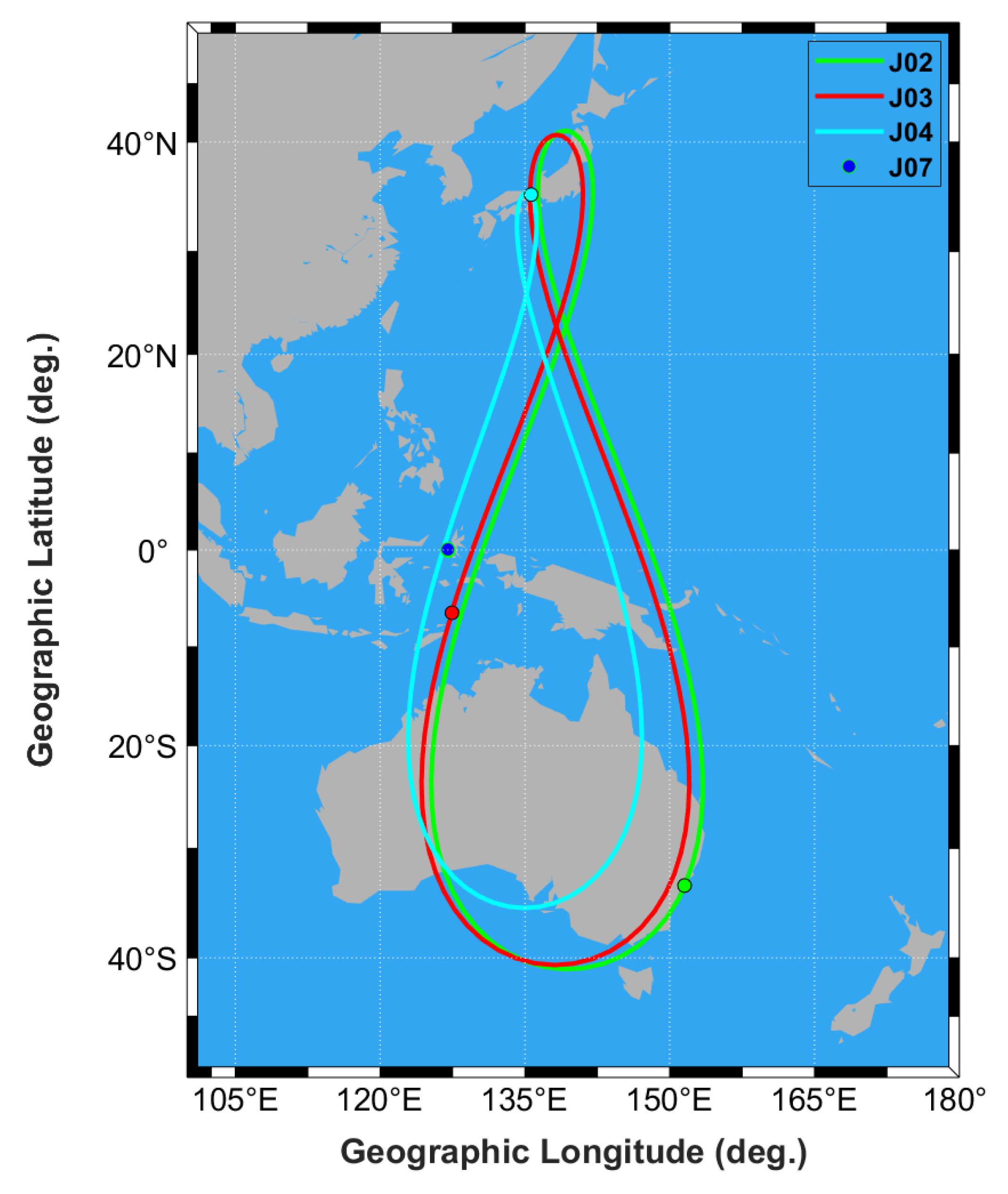
Figure 2.
The distribution of nine GNSS reference stations for the QZSS TEC estimation. The red circles denote the locations of GNSS stations.
Figure 2.
The distribution of nine GNSS reference stations for the QZSS TEC estimation. The red circles denote the locations of GNSS stations.
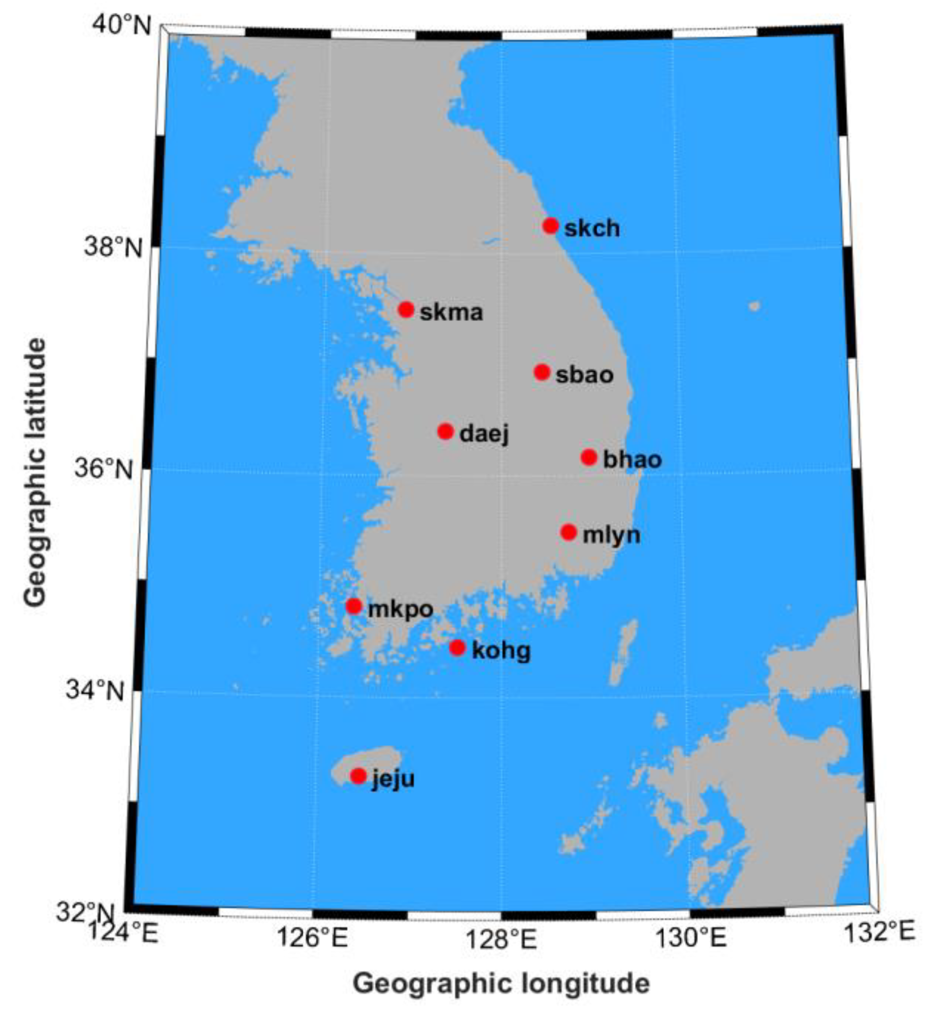
Figure 3.
Spatial distribution of the nine GNSS reference stations used for QZSS TEC estimation. The filled red circles represent the locations of the GNSS stations, while the green lines indicate the ionospheric pierce points (IPPs) corresponding to the QZSS satellite signals.
Figure 3.
Spatial distribution of the nine GNSS reference stations used for QZSS TEC estimation. The filled red circles represent the locations of the GNSS stations, while the green lines indicate the ionospheric pierce points (IPPs) corresponding to the QZSS satellite signals.
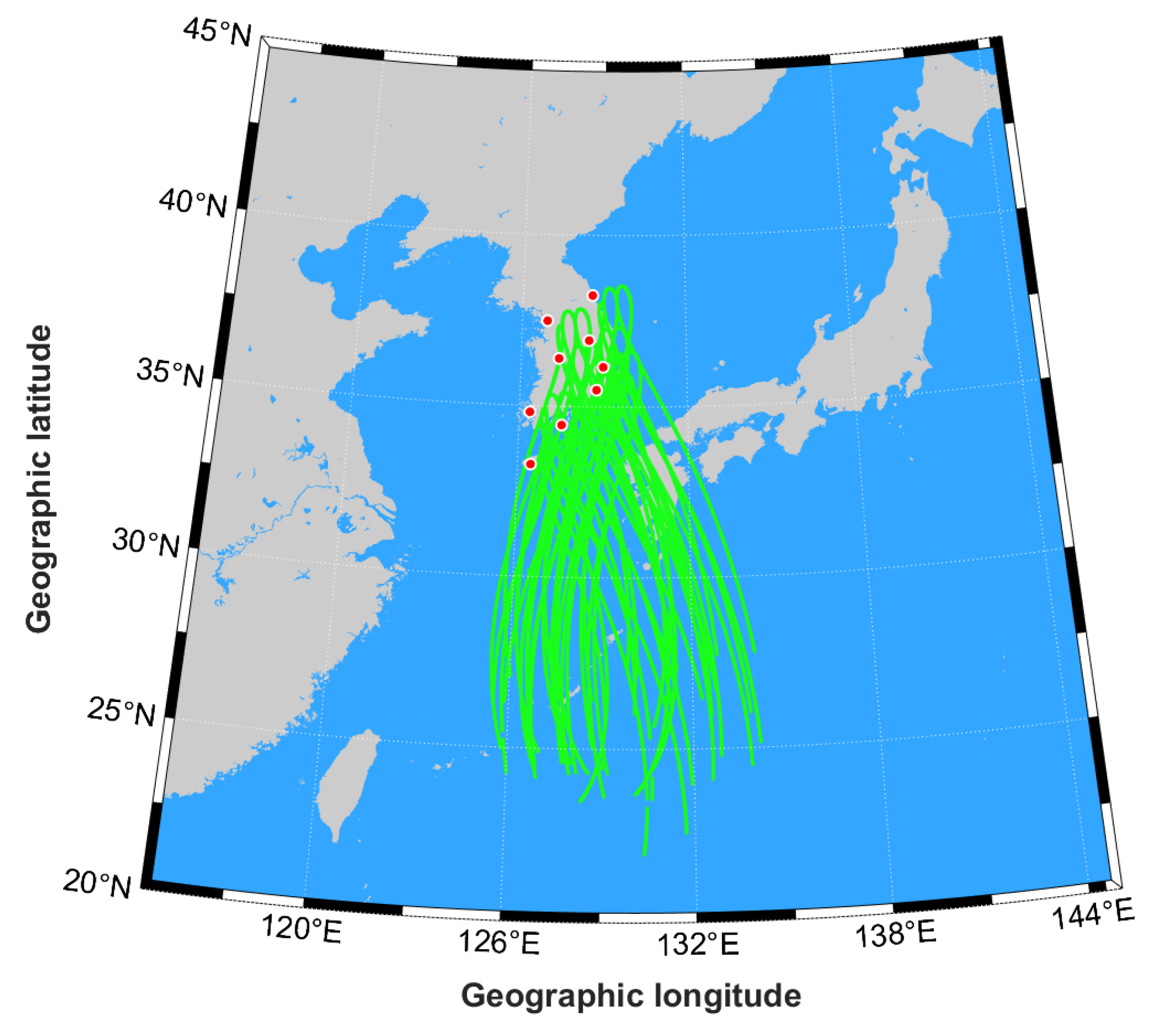
Figure 4.
Time series of DCBs for QZSS satellites from DOY 1 to 181, 2024. From top to bottom, the panels sequentially show a) C1C-C2X DCBs, b) C1C-C5X DCBs, and c) C2X-C5X DCBs, respectively.
Figure 4.
Time series of DCBs for QZSS satellites from DOY 1 to 181, 2024. From top to bottom, the panels sequentially show a) C1C-C2X DCBs, b) C1C-C5X DCBs, and c) C2X-C5X DCBs, respectively.
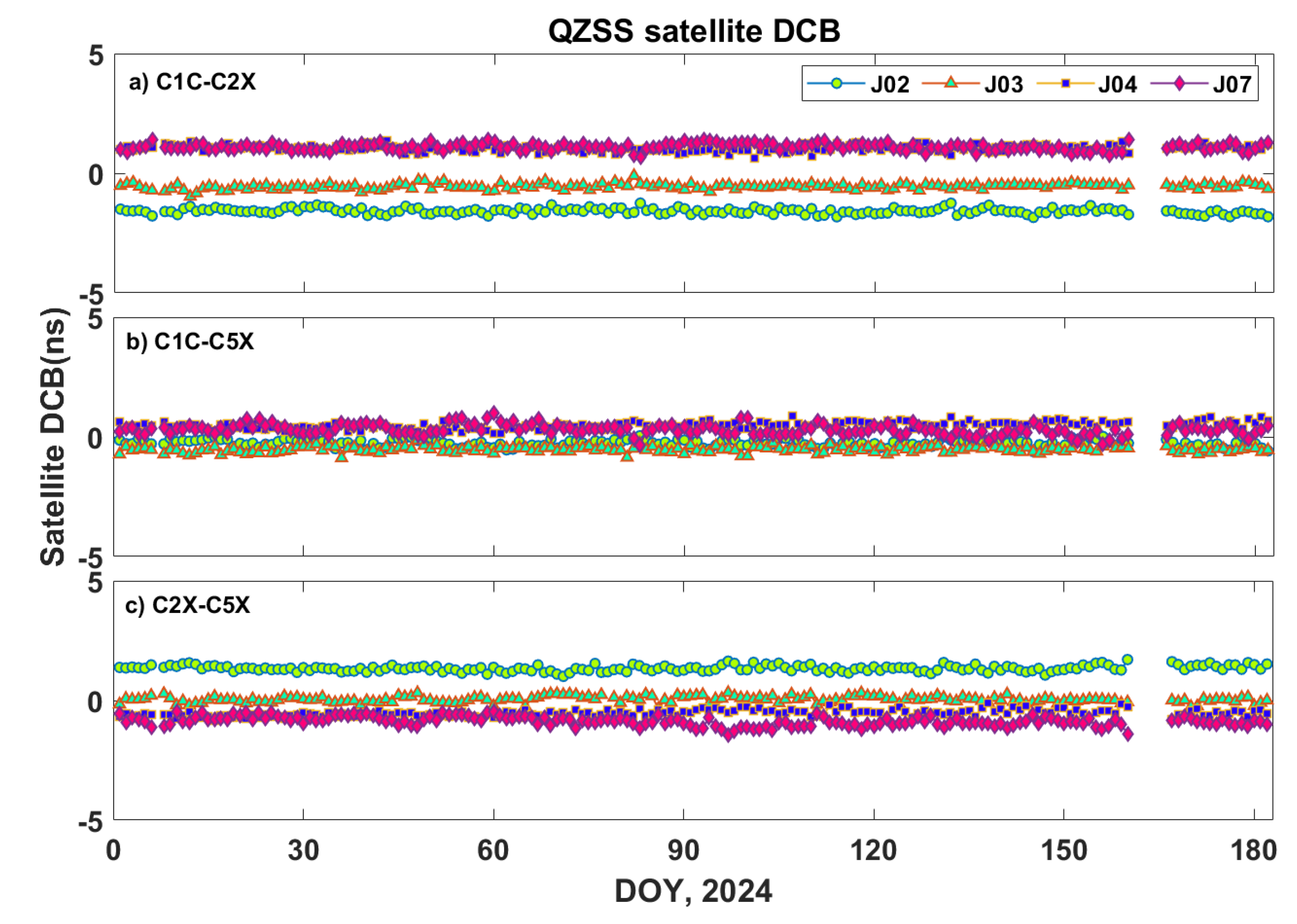
Figure 5.
Summaries of the QZSS satellite DCB values corresponding to the time series shown in Figure 4. Panels (a), (b), and (c) present the mean and RMS values of the DCBs for the C1C-C2X, C1C-C5X, and C2X-C5X combinations, respectively. The blue error bars represent the RMS values associated with each satellite’s DCB estimate.
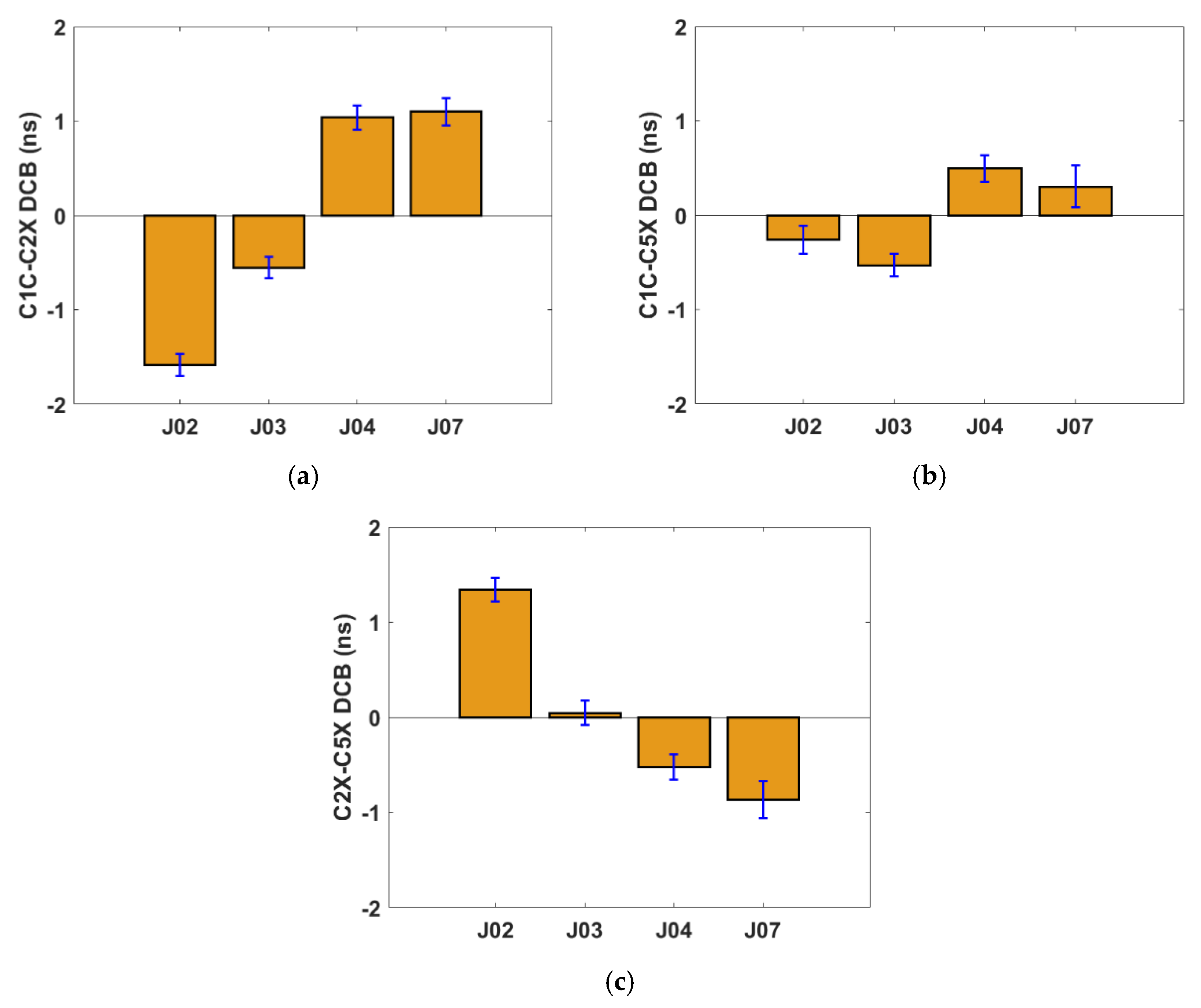
Figure 6.
The TEC time series estimated by three different signal combinations of QZSS satellite J07 at the ‘daej’ station from DOY 1 to 182 in 2024. L1-L2, L1-L5, and L2-L5 combinations are represented by red, blue, and green dots, respectively.
Figure 6.
The TEC time series estimated by three different signal combinations of QZSS satellite J07 at the ‘daej’ station from DOY 1 to 182 in 2024. L1-L2, L1-L5, and L2-L5 combinations are represented by red, blue, and green dots, respectively.
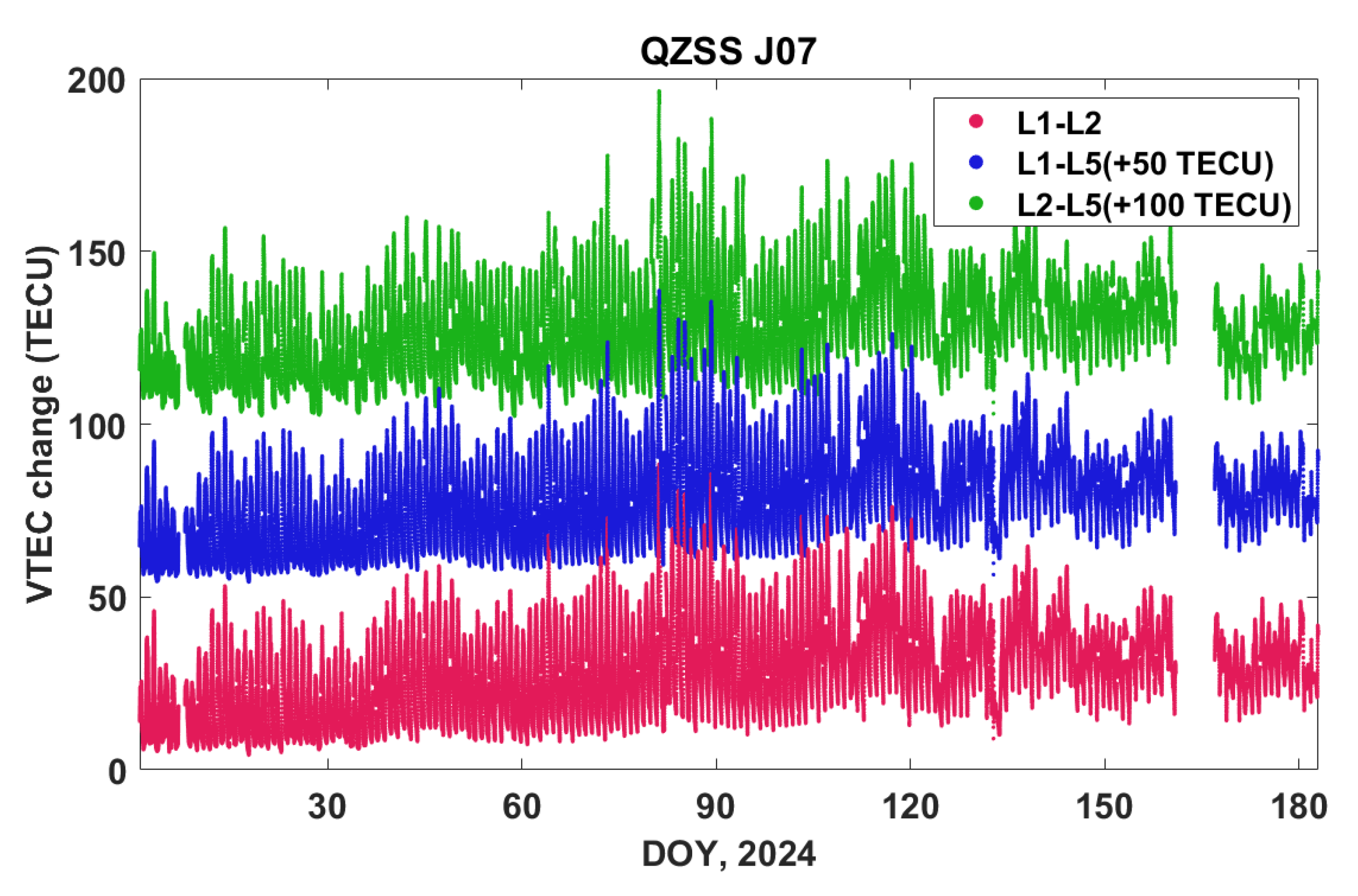
Figure 7.
Comparison between QZSS-derived TEC and the CODE GIM TEC from DOY 1 to 182 in 2024. a) L1–L2, b) L1–L5, and c) L2–L5 combinations. In the subplots, the QZSS and CODE GIM are represented by gray dots and red dashed lines, respectively.
Figure 7.
Comparison between QZSS-derived TEC and the CODE GIM TEC from DOY 1 to 182 in 2024. a) L1–L2, b) L1–L5, and c) L2–L5 combinations. In the subplots, the QZSS and CODE GIM are represented by gray dots and red dashed lines, respectively.
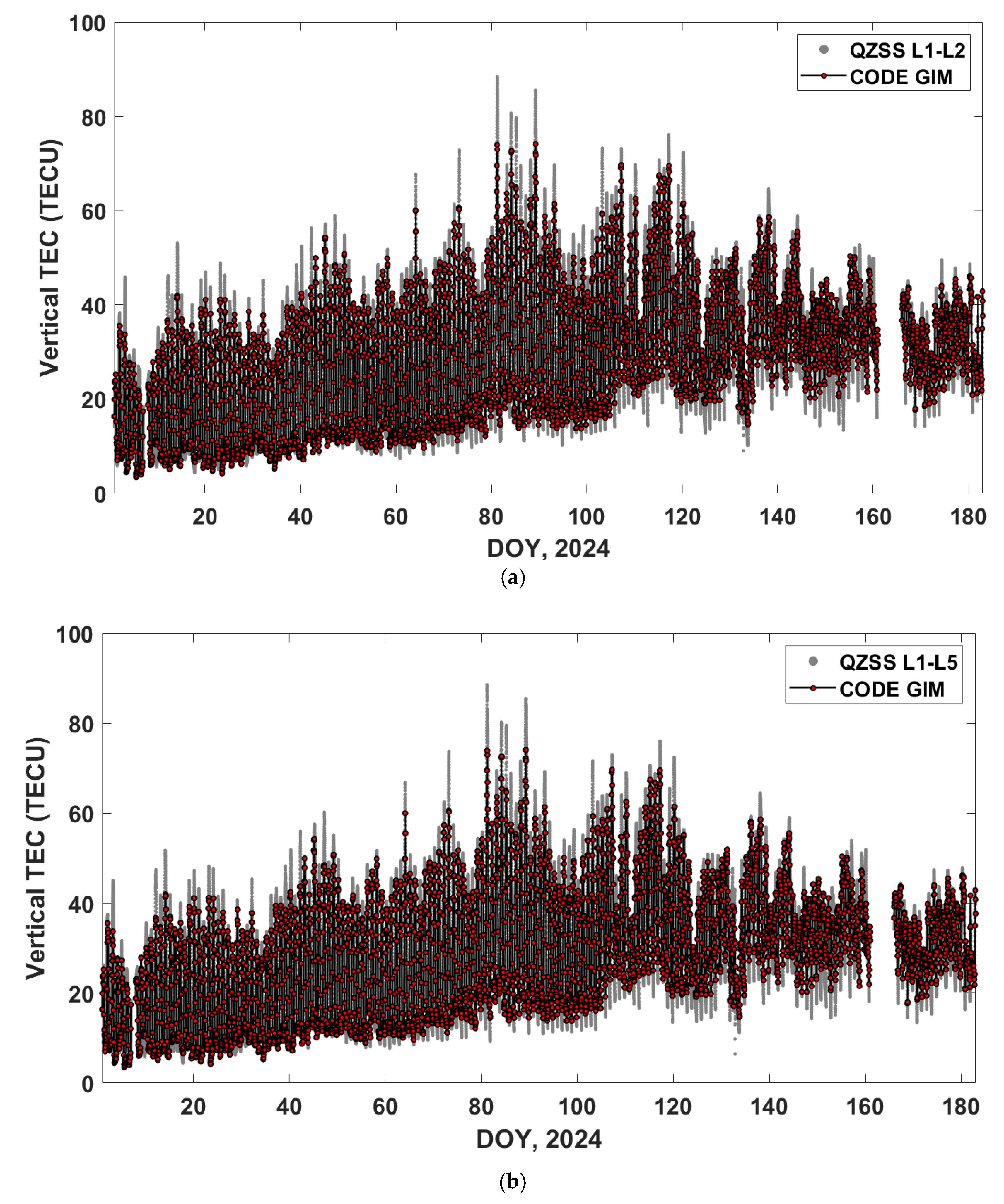
Figure 8.
The TEC difference time series between the L1-L2 and L1-L5 combinations from DOY 1 to 182 in 2024. The blue dots represent the TEC difference. The linear fit and the 95% confidence level for them are shown as red solid lines and cyan dashed lines, respectively.
Figure 8.
The TEC difference time series between the L1-L2 and L1-L5 combinations from DOY 1 to 182 in 2024. The blue dots represent the TEC difference. The linear fit and the 95% confidence level for them are shown as red solid lines and cyan dashed lines, respectively.
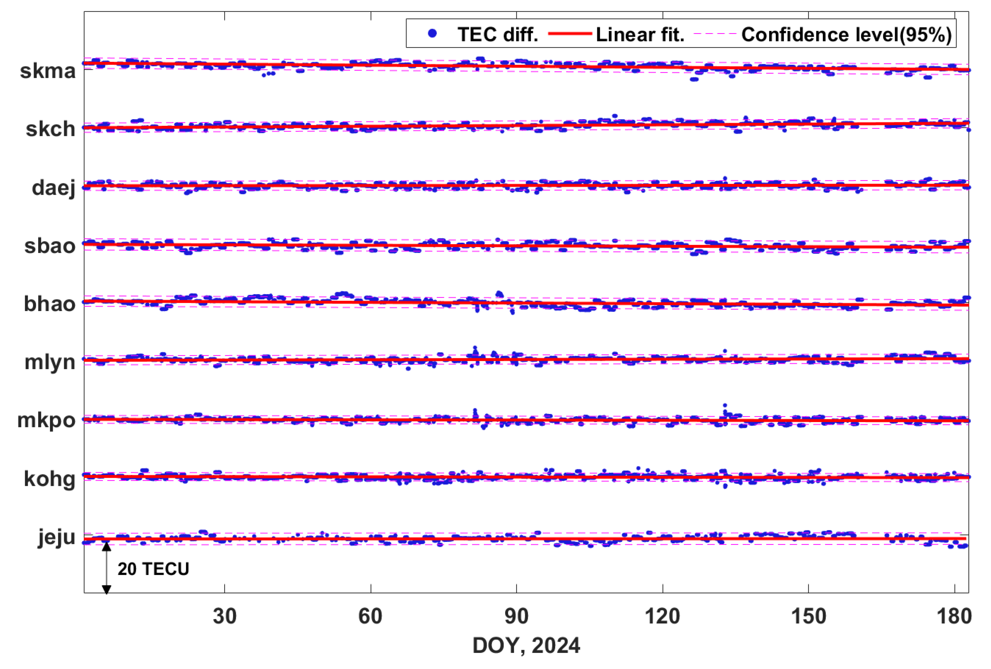
Figure 9.
The TEC difference time series between the L2-L5 and L1-L5 combinations from DOY 1 to 182 in 2024. The blue dots represent the TEC difference. The linear fit and the 95% confidence level for them are shown as red solid lines and cyan dashed lines, respectively.
Figure 9.
The TEC difference time series between the L2-L5 and L1-L5 combinations from DOY 1 to 182 in 2024. The blue dots represent the TEC difference. The linear fit and the 95% confidence level for them are shown as red solid lines and cyan dashed lines, respectively.
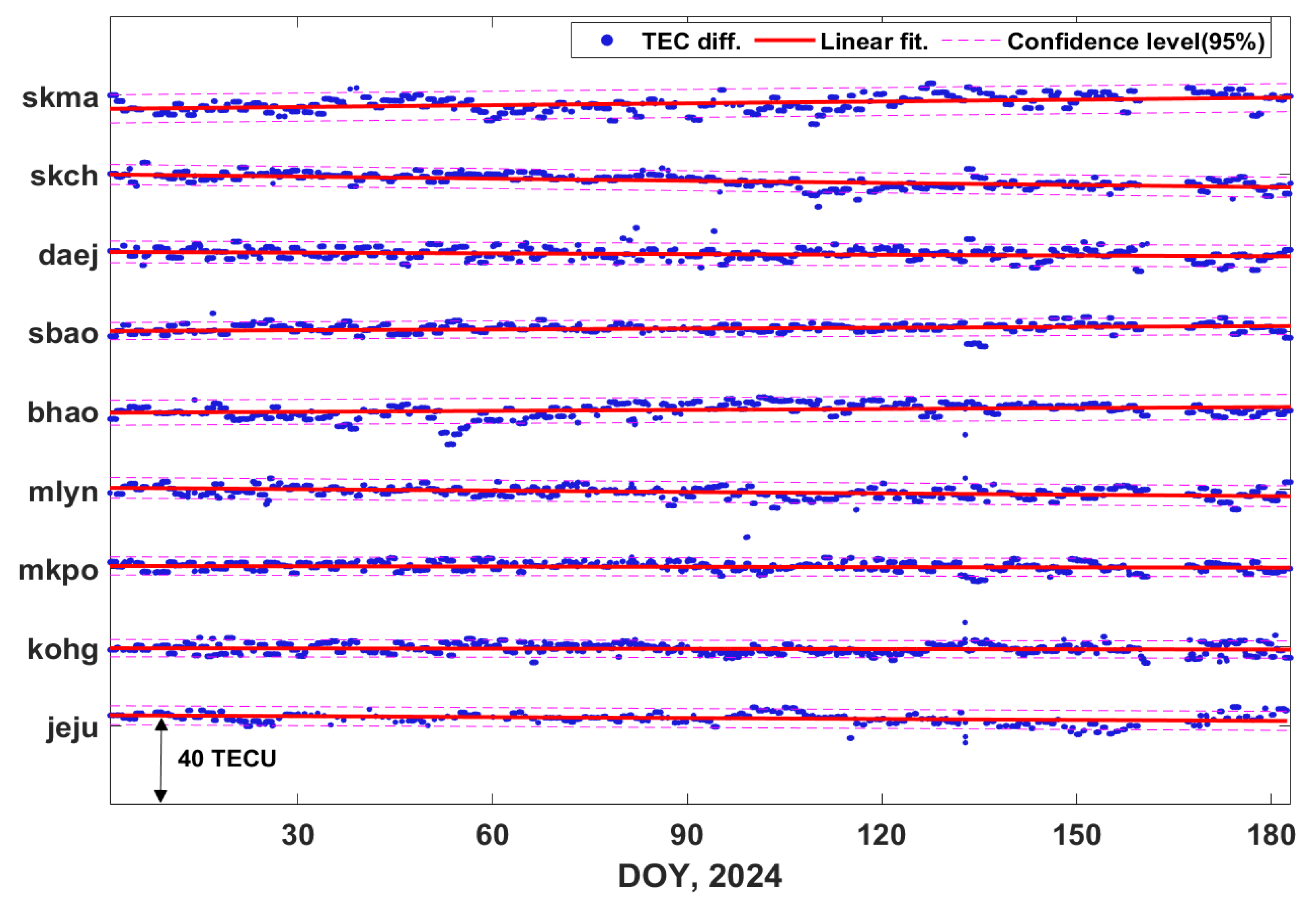
Figure 10.
The ROT values derived from three different signal combinations observed at the ‘daej’ station on January 1, 2024. The L1-L2, L1-L5, and L2-L5 combinations are represented by red, blue, and gray lines, respectively.
Figure 10.
The ROT values derived from three different signal combinations observed at the ‘daej’ station on January 1, 2024. The L1-L2, L1-L5, and L2-L5 combinations are represented by red, blue, and gray lines, respectively.
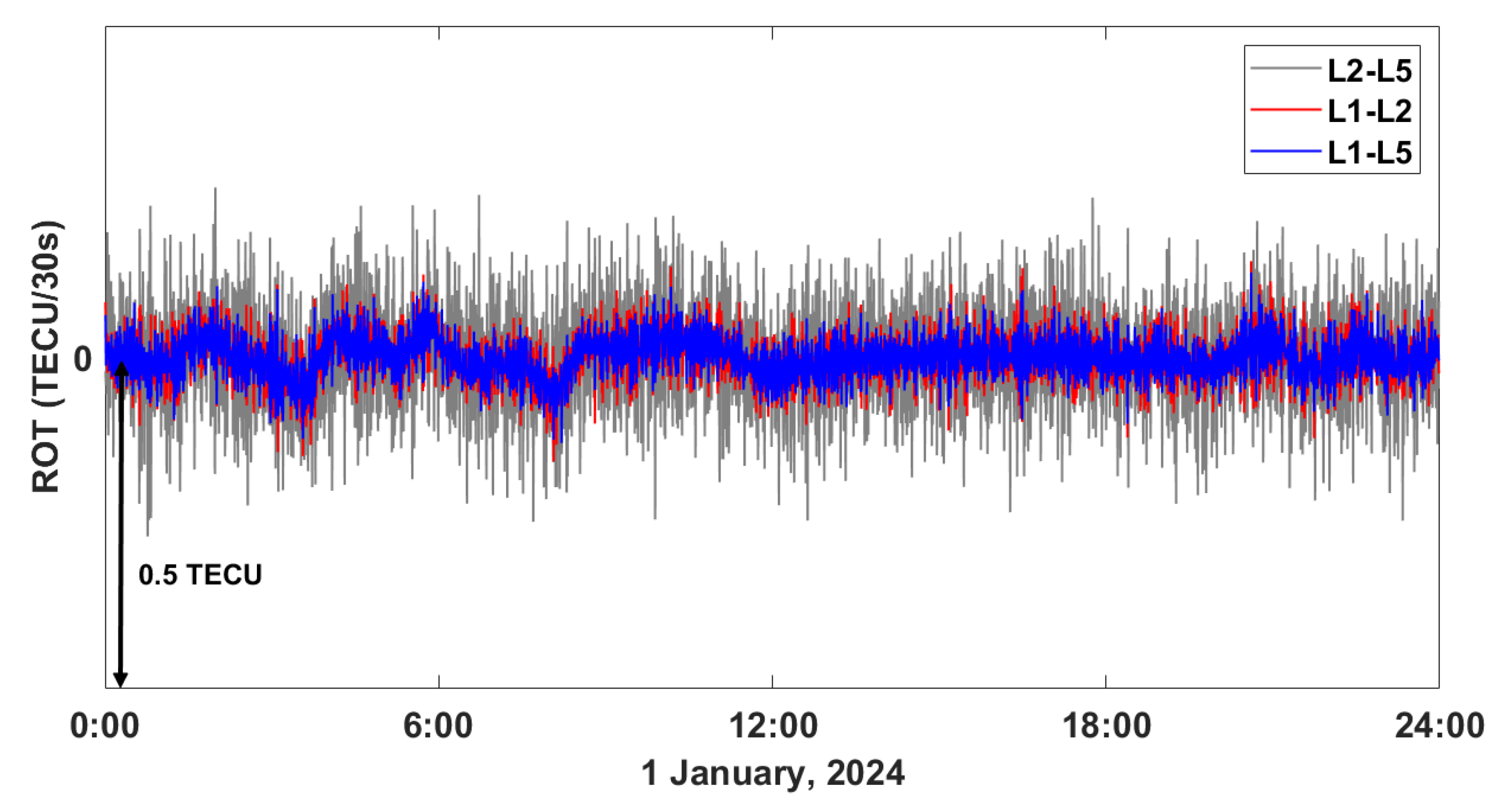
Figure 11.
Time series of ROT observed at nine GNSS stations from January 1 to 6, 2024.
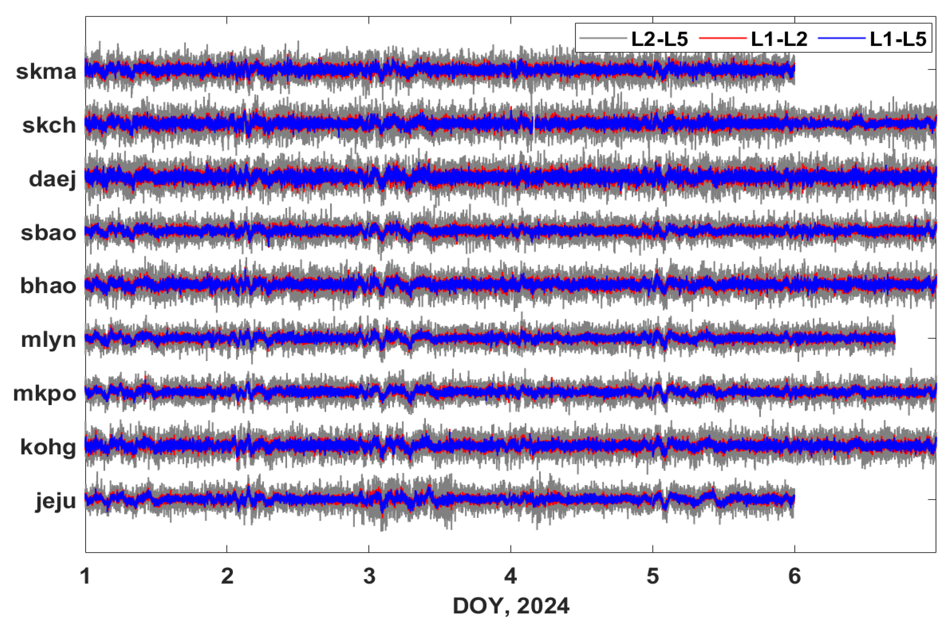

Table 1.
The types of receiver and antenna at the GNSS stations.
| Site name |
Receiver type | Antenna type | Geographic latitude (degrees) | Geographic longitude (degrees) |
|---|---|---|---|---|
| skch | TRIMBLE NetR9 | TRM59800.00 SCIS | 38.25° N | 128.56° E |
| skma | TRIMBLE NetR9 | TRM59800.00 SCIS | 37.49° N | 126.91° E |
| sbao | TRIMBLE NetR9 | TRM59800.00 SCIS | 36.93° N | 128.45° E |
| daej | TRIMBLE NetR9 | TRM59800.00 SCIS | 36.39° N | 127.37° E |
| bhao | TRIMBLE NetR9 | TRM59800.00 SCIS | 36.16° N | 128.97° E |
| mlyn | TRIMBLE NetR9 | TRM59800.00 SCIS | 35.49° N | 128.74° E |
| mkpo | TRIMBLE NetR9 | TRM59800.00 SCIS | 34.81° N | 126.38° E |
| kohg | TRIMBLE NetR9 | TRM59800.00 SCIS | 34.45° N | 127.51° E |
| jeju | TRIMBLE NetR9 | TRM59800.00 SCIS | 33.28° N | 126.46° E |
Table 2.
QZSS observation types at selected GNSS stations.
| Signal | Observation types |
|---|---|
| L1 | C1C, L1C, C1X, L1X, C1Z, L1Z |
| L2 | C2X, L2X |
| L5 | C5X, L5X |
Table 3.
Average and RMS values of satellite DCBs with three different signal combinations.
| PRN | Signal combination | Average value (ns) | RMS value (ns) |
|---|---|---|---|
| J02 | C1C-C2X | -1.58 | 0.11 |
| C1C-C5X | -0.26 | 0.14 | |
| C2X-C5X | 1.34 | 0.12 | |
| J03 | C1C-C2X | -0.55 | 0.11 |
| C1C-C5X | -0.53 | 0.12 | |
| C2X-C5X | 0.04 | 0.12 | |
| J04 | C1C-C2X | 1.03 | 0.12 |
| C1C-C5X | 0.49 | 0.14 | |
| C2X-C5X | -0.52 | 0.13 | |
| J07 | C1C-C2X | 1.10 | 0.14 |
| C1C-C5X | 0.30 | 0.22 | |
| C2X-C5X | -0.86 | 0.19 |
Table 4.
RMS values of ROT derived from three different GNSS signal combinations (L1-L2, L1-L5, and L2-L5) observed at the GNSS stations from January 1 to 6, 2024.
Table 4.
RMS values of ROT derived from three different GNSS signal combinations (L1-L2, L1-L5, and L2-L5) observed at the GNSS stations from January 1 to 6, 2024.
| Site name | Signals | RMS value (TECU) |
|---|---|---|
| L1-L2 | 0.034 | |
| skma | L1-L5 | 0.028 |
| L2-L5 | 0.073 | |
| L1-L2 | 0.036 | |
| skch | L1-L5 | 0.030 |
| L2-L5 | 0.079 | |
| L1-L2 | 0.039 | |
| daej | L1-L5 | 0.033 |
| L2-L5 | 0.083 | |
| L1-L2 | 0.029 | |
| sbao | L1-L5 | 0.025 |
| L2-L5 | 0.064 | |
| L1-L2 | 0.033 | |
| bhao | L1-L5 | 0.028 |
| L2-L5 | 0.073 | |
| L1-L2 | 0.028 | |
| mlyn | L1-L5 | 0.025 |
| L2-L5 | 0.059 | |
| L1-L2 | 0.028 | |
| mkpo | L1-L5 | 0.025 |
| L2-L5 | 0.059 | |
| L1-L2 | 0.035 | |
| kohg | L1-L5 | 0.029 |
| L2-L5 | 0.072 | |
| L1-L2 | 0.028 | |
| jeju | L1-L5 | 0.025 |
| L2-L5 | 0.059 |
Disclaimer/Publisher’s Note: The statements, opinions and data contained in all publications are solely those of the individual author(s) and contributor(s) and not of MDPI and/or the editor(s). MDPI and/or the editor(s) disclaim responsibility for any injury to people or property resulting from any ideas, methods, instructions or products referred to in the content. |
© 2025 by the authors. Licensee MDPI, Basel, Switzerland. This article is an open access article distributed under the terms and conditions of the Creative Commons Attribution (CC BY) license (http://creativecommons.org/licenses/by/4.0/).
Copyright: This open access article is published under a Creative Commons CC BY 4.0 license, which permit the free download, distribution, and reuse, provided that the author and preprint are cited in any reuse.


