An Extended Dirac Equation in Curved Spacetime and Applications to Quantum Electromagnetic Processes: A Metric-Internalization Approach Using a 256 × 256 Matrix Representation

1. Introduction

1.1. Background and Motivation

In relativistic quantum mechanics, the Dirac equation describes the motion of spin-$1/2$ particles such as electrons. In flat spacetime (special-relativistic Minkowski spacetime) it is a well-established theory [1,2]. However, how to extend the Dirac equation to curved spacetime in the presence of a gravitational field remains an important research topic [3,4].

The standard approach to spinor fields in curved spacetime introduces a vierbein (tetrad) ${e^a}_{\mu }\left(x\right)$ and a spin connection${{\omega }_{\mu }}^{ab}\left(x\right)$ [5,6]. While theoretically complete, practical scattering calculations often face the following difficulties:

• The choice of vierbein is not unique, and calculations can become cumbersome.
• Introducing the spin connection can obscure the correspondence with flat-spacetime calculation rules.
• Automation of numerical calculations becomes difficult.

1.2. Our Approach: Internalizing the Metric into Matrices

To avoid these difficulties, we propose a new approach. The basic idea is to embed the spacetime metric $g_{\mu \nu }\left(x\right)$ directly into gamma matrices. This makes it possible to construct a Dirac equation in curved spacetime without explicitly introducing a vierbein.

Specifically, we extend the conventional $4\times 4$ gamma matrices ${\gamma }^{\mu }$ (four matrices) and introduce sixteen $256\times 256$ matrices ${\Gamma }_{\mu }^{\nu }$. Key points are:

• The spacetime dimension remains four (no extra dimensions are introduced).
• The number “16” corresponds to the number of basis elements of the four-dimensional Dirac algebra ($2^4=16$).
• The metric tensor is incorporated as a coefficient of the matrices.

1.3. Outline of the Formulation

The formulation proceeds in the following steps.

1.3.0.1. Step 1: Introduction of two-index gamma matrices

We construct constant (position-independent) basis matrices ${\Gamma }_{\mu }^{\nu }$ ($\mu ,\nu =0,1,2,3$) as $256\times 256$ matrices.

1.3.0.2. Step 2: Metric internalization

Using the spacetime metric $g_{\mu \nu }\left(x\right)$, we define the position-dependent gamma matrices by

$${\Gamma }_{\mu \nu }\left(x\right):={\Gamma }_{\mu }{}^{\rho }{g}_{\rho \nu }\left(x\right).$$

(1)

In this way the metric information is internalized into the gamma matrices (Equation (1)).

1.3.0.3. Step 3: Construction of effective gamma matrices

By summing the above sixteen matrices along the column direction, we define the effective gamma matrices

$${\widehat{\Gamma }}_{\nu }\left(x\right):=\sum _{\mu =0}^3{\Gamma }_{\mu \nu }\left(x\right).$$

(2)

These four effective gamma matrices are the basic building blocks for the Dirac equation in curved spacetime.

1.3.0.4. Step 4: Dirac operator

With the effective gamma matrices, we extend the slash notation as

$$\cancel{p}\left(x\right):={\widehat{\Gamma }}_{\nu }\left(x\right)p^{\nu },$$

(3)

and define the Dirac operator as

$$D\left(x\right):={\widehat{\Gamma }}_{\nu }\left(x\right){\partial }^{\nu }.$$

(4)

The slash notation (Equation (3)) and Dirac operator (Equation (4)) form the basis of our extended formalism.

1.4. Consistency with Flat Spacetime

A key property of this approach is that it reproduces standard results exactly in the flat-spacetime limit. When the metric approaches the Minkowski metric, $g_{\mu \nu }\left(x\right)\to {\eta }_{\mu \nu }$,

$${\Gamma }_{\mu \nu }\left(x\right)\to {\Gamma }_{\mu }{}^{\rho }\eta _{\rho \nu },{\widehat{\Gamma }}_{\nu }\left(x\right)\to \sum _{\mu }{\Gamma }_{\mu }{}^{\rho }\eta _{\rho \nu },$$

and the results obtained with the $256\times 256$ representation coincide with the standard $4\times 4$ representation under an appropriate normalization.

We verified this consistency numerically for all scattering processes treated in this paper:

• Compton scattering (Section 5);
• Muon-pair production (Appendix B);
• Møller scattering (Appendix C);
• Bhabha scattering (Appendix D).

In each case, we confirm agreement with classical results, including the Klein–Nishina formula [7] and related standard QED results [1,2,8].

1.5. Main Contributions

The main contributions of this paper are as follows:

(i)

New formulation: Construction of two-index gamma matrices that embed the metric directly, and introduction of a matrix-valued Dirac operator based on effective gammas ${\widehat{\Gamma }}^{\mu }\left(x\right)$ (Equation (2)).

(ii)

Computational organization: Presentation of Feynman rules derived from the extended QED Lagrangian (Equation (6)) and a procedure suitable for automation.

(iii)

Numerical validation: Trial calculations using metrics with off-diagonal components (toy models) show characteristic corrections in the angular dependence of differential cross sections, while confirming exact agreement in the flat limit [9,10,11].

1.6. Comparison Between Conventional and Extended Dirac Equations

To visualize the structure of the proposed approach, we compare the conventional and extended Dirac equations in matrix form.

Conventional Dirac equation (flat spacetime)

In flat spacetime, the Dirac equation uses four $4\times 4$ gamma matrices ${\gamma }^{\mu }$:

$$\left(i{\gamma }^{\mu }{\partial }_{\mu }-m\right)\psi \left(x\right)=0.$$

The gamma matrices satisfy

$$\{{\gamma }^{\mu },{\gamma }^{\nu }\}=2{\eta }^{\mu \nu }{I}_4,{\eta }_{\mu \nu }=\mathrm{diag}(+1,-1,-1,-1).$$

In matrix form,

$$\begin{array}{cc}\hfill & \underset{4\times 4\mathrm{matrices};\mathrm{four}\mathrm{gammas}}{\underbrace{\left(\mathbf{Conventional}\right)}}i\underset{{\displaystyle \mathrm{diagonal}\mathrm{only}}}{\underbrace{\left[\begin{array}{cccc}{\gamma }_0^0& 0& 0& 0\\ 0& {\gamma }_1^1& 0& 0\\ 0& 0& {\gamma }_2^2& 0\\ 0& 0& 0& {\gamma }_3^3\end{array}\right]}}\underset{{\displaystyle {\eta }_{\mu \nu }(\mathrm{Minkowski}\mathrm{metric})}}{\underbrace{\left[\begin{array}{cccc}+1& 0& 0& 0\\ 0& -1& 0& 0\\ 0& 0& -1& 0\\ 0& 0& 0& -1\end{array}\right]}}\left[\begin{array}{c}{\partial }^0\\ {\partial }^1\\ {\partial }^2\\ {\partial }^3\end{array}\right]-m{I}_4\hfill \end{array}$$

(5)

Because ${\eta }_{\mu \nu }$ is diagonal in flat spacetime, a diagonal placement of gamma matrices is sufficient (Equation (5)).

Extended Dirac equation (curved spacetime)

In curved spacetime, the metric $g_{\mu \nu }\left(x\right)$ generally has off-diagonal components. To accommodate this, we employ sixteen $256\times 256$ matrices ${\Gamma }_{\mu }^{\nu }$ and multiply them directly by the metric:

$$\begin{array}{cc}\hfill & \underset{256\times 256\mathrm{matrices};\mathrm{sixteen}\mathrm{gammas}}{\underbrace{\left(\mathbf{Extended}\right)}}\hfill \\ \hfill & i\underset{16\mathrm{basis}\mathrm{matrices}\left(256\times 256\right)}{\underbrace{\left[\begin{array}{cccc}{\Gamma }_0^0& {\Gamma }_0^1& {\Gamma }_0^2& {\Gamma }_0^3\\ {\Gamma }_1^0& {\Gamma }_1^1& {\Gamma }_1^2& {\Gamma }_1^3\\ {\Gamma }_2^0& {\Gamma }_2^1& {\Gamma }_2^2& {\Gamma }_2^3\\ {\Gamma }_3^0& {\Gamma }_3^1& {\Gamma }_3^2& {\Gamma }_3^3\end{array}\right]}}\underset{\mathrm{general}\mathrm{metric}\mathrm{tensor}(\mathrm{with}\mathrm{off}-\mathrm{diagonal}\mathrm{components})}{\underbrace{\left[\begin{array}{cccc}{g}_{00}& g_{01}& g_{02}& g_{03}\\ g_{10}& g_{11}& g_{12}& g_{13}\\ g_{20}& g_{21}& g_{22}& g_{23}\\ g_{30}& g_{31}& g_{32}& g_{33}\end{array}\right]}}\left[\begin{array}{c}{\partial }^0\\ {\partial }^1\\ {\partial }^2\\ {\partial }^3\end{array}\right]-m{I}_{256}\hfill \\ \hfill & =i{\Gamma }_{\mu }{}^{\rho }g_{\rho \nu }\left(x\right){\partial }^{\nu }-m{I}_{256}=i{\Gamma }_{\mu \nu }\left(x\right){\partial }^{\nu }-m{I}_{256}\hfill \end{array}$$

(6)

where ${\Gamma }_{\mu \nu }\left(x\right):={\Gamma }_{\mu }{}^{\rho }g_{\rho \nu }\left(x\right)$.

Advantages of this construction are:

• Off-diagonal metric components are incorporated naturally.
• No explicit vierbein is required.
• Calculation rules are unified in terms of matrix products and traces.
• The flat limit reduces automatically to standard results.

1.7. Organization of the Paper

The remainder of this paper is organized as follows. Section 2 presents the explicit construction of the $256\times 256$ matrix representation. Section 3 discusses consistency under general coordinate transformations. Section 4 introduces the extended QED Lagrangian and the associated Feynman rules. Section 5 presents representative scattering calculations (Compton scattering) and compares with the flat-spacetime results. Section 6 discusses the focus, scope, advantages, and limitations of the method, and Section 7 concludes. Additional processes (muon-pair production, Møller scattering, and Bhabha scattering) and the Mathematica code repository are provided in the appendices.

2. Construction of the $256\times 256$ Matrix Representation

2.1. Why a $256\times 256$ Representation with 16 Basis Matrices?

This section explains the construction of the $256\times 256$ matrix representation and clarifies why it is needed and what mathematical background motivates it.

Number of basis elements of the Dirac algebra

In four-dimensional spacacetime, the Dirac (gamma-matrix) algebra has the following 16 independent basis elements:

$$\{I,{\gamma }^{\mu },{\gamma }^{\mu }{\gamma }^{\nu }(\mu <\nu ),{\gamma }^{\mu }{\gamma }^{\nu }{\gamma }^{\rho }(\mu <\nu <\rho ),{\gamma }^5\}.$$

This is $2^4=16$ basis elements. In the conventional $4\times 4$ representation, these basis elements are represented by products of the four ${\gamma }^{\mu }$.

Motivation for a two-index representation

In the present approach, we multiply the metric $g_{\mu \nu }\left(x\right)$ directly into gamma matrices. For this purpose, we label the gamma matrices by two indices$(\mu ,\nu )$. Since $\mu ,\nu =0,1,2,3$, there are $4\times 4=16$ combinations, corresponding to the “sixteen basis matrices” used here.

Why $256\times 256$?

To realize each basis matrix ${\Gamma }_{\mu }^{\nu }$ explicitly, we use Kronecker (tensor) products of Pauli matrices. Taking an 8-fold tensor product of $2\times 2$ matrices yields

$$2^8=256,$$

hence a $256\times 256$ matrix representation. This construction provides 16 mutually independent basis matrices and ensures that the required anticommutation relations hold.

2.2. Kronecker-Product Construction Using Pauli Matrices

We use the $2\times 2$ identity matrix e and the Pauli matrices

$${\sigma }_x=\left(\begin{array}{cc}0& 1\\ 1& 0\end{array}\right),{\sigma }_y=\left(\begin{array}{cc}0& -i\\ i& 0\end{array}\right),{\sigma }_z=\left(\begin{array}{cc}1& 0\\ 0& -1\end{array}\right)$$

as building blocks, and construct the basis matrices by an eight-fold Kronecker product (⊗).

$$\begin{array}{cc}\hfill {\Gamma }_0^0& ={\sigma }_x\otimes {\sigma }_x\otimes {\sigma }_x\otimes {\sigma }_x\otimes {\sigma }_x\otimes {\sigma }_x\otimes {\sigma }_x\otimes {\sigma }_x\hfill \\ \hfill {\Gamma }_0^1& =i{\sigma }_x\otimes {\sigma }_x\otimes {\sigma }_x\otimes {\sigma }_x\otimes {\sigma }_x\otimes {\sigma }_x\otimes {\sigma }_x\otimes {\sigma }_y\hfill \\ \hfill {\Gamma }_0^2& =i{\sigma }_x\otimes {\sigma }_x\otimes {\sigma }_x\otimes {\sigma }_x\otimes {\sigma }_x\otimes {\sigma }_x\otimes {\sigma }_x\otimes {\sigma }_z\hfill \\ \hfill {\Gamma }_0^3& =i{\sigma }_y\otimes {\sigma }_z\otimes {\sigma }_z\otimes {\sigma }_z\otimes {\sigma }_z\otimes {\sigma }_z\otimes {\sigma }_z\otimes {\sigma }_z\hfill \\ \hfill {\Gamma }_1^0& =i{\sigma }_x\otimes {\sigma }_x\otimes {\sigma }_y\otimes {\sigma }_z\otimes {\sigma }_z\otimes {\sigma }_z\otimes {\sigma }_z\otimes {\sigma }_z\hfill \\ \hfill {\Gamma }_1^1& =i{\sigma }_x\otimes {\sigma }_x\otimes {\sigma }_x\otimes {\sigma }_x\otimes {\sigma }_z\otimes {\sigma }_z\otimes {\sigma }_z\otimes {\sigma }_z\hfill \\ \hfill {\Gamma }_1^2& =i{\sigma }_x\otimes {\sigma }_x\otimes {\sigma }_x\otimes {\sigma }_x\otimes {\sigma }_x\otimes {\sigma }_z\otimes {\sigma }_z\otimes {\sigma }_z\hfill \\ \hfill {\Gamma }_1^3& =i{\sigma }_x\otimes {\sigma }_x\otimes {\sigma }_x\otimes {\sigma }_x\otimes {\sigma }_x\otimes {\sigma }_x\otimes {\sigma }_y\otimes {\sigma }_z\hfill \\ \hfill {\Gamma }_2^0& =i{\sigma }_z\otimes {\sigma }_z\otimes {\sigma }_z\otimes {\sigma }_z\otimes {\sigma }_z\otimes {\sigma }_z\otimes {\sigma }_z\otimes {\sigma }_z\hfill \\ \hfill {\Gamma }_2^1& =i{\sigma }_x\otimes {\sigma }_x\otimes {\sigma }_x\otimes {\sigma }_x\otimes {\sigma }_y\otimes {\sigma }_z\otimes {\sigma }_z\otimes {\sigma }_z\hfill \\ \hfill {\Gamma }_2^2& =i{\sigma }_x\otimes {\sigma }_x\otimes {\sigma }_x\otimes {\sigma }_y\otimes {\sigma }_z\otimes {\sigma }_z\otimes {\sigma }_z\otimes {\sigma }_z\hfill \\ \hfill {\Gamma }_2^3& =i{\sigma }_x\otimes {\sigma }_x\otimes {\sigma }_x\otimes {\sigma }_x\otimes {\sigma }_x\otimes {\sigma }_y\otimes {\sigma }_z\otimes {\sigma }_z\hfill \\ \hfill {\Gamma }_3^0& =i{\sigma }_x\otimes {\sigma }_y\otimes {\sigma }_z\otimes {\sigma }_z\otimes {\sigma }_z\otimes {\sigma }_z\otimes {\sigma }_z\otimes {\sigma }_z\hfill \\ \hfill {\Gamma }_3^1& =i{\sigma }_x\otimes {\sigma }_z\otimes {\sigma }_z\otimes {\sigma }_z\otimes {\sigma }_z\otimes {\sigma }_z\otimes {\sigma }_z\otimes {\sigma }_z\hfill \\ \hfill {\Gamma }_3^2& =i{\sigma }_x\otimes {\sigma }_x\otimes {\sigma }_x\otimes {\sigma }_z\otimes {\sigma }_z\otimes {\sigma }_z\otimes {\sigma }_z\otimes {\sigma }_z\hfill \\ \hfill {\Gamma }_3^3& =i{\sigma }_x\otimes {\sigma }_x\otimes {\sigma }_z\otimes {\sigma }_z\otimes {\sigma }_z\otimes {\sigma }_z\otimes {\sigma }_z\otimes {\sigma }_z\hfill \end{array}$$

(7)

This construction follows standard references on Clifford algebras and spinors [12,13,14,15].

2.3. Anticommutation Relations

The sixteen basis matrices satisfy the anticommutation relation

$$\begin{array}{c}\hfill \begin{array}{|c|}\hline \{{\Gamma }_{\mu }{}^{\nu },{\Gamma }_{\rho }{}^{\sigma }\}=2{\delta }^{\nu }{}_{\sigma }{\eta }_{\mu \rho }{I}_{256}\\ \hline\end{array}\end{array}$$

(8)

which can be interpreted as follows:

• If the right indices match ($\nu =\sigma$): for each fixed column index, $\{{\Gamma }_{\mu }{}^{\nu },{\Gamma }_{\rho }{}^{\nu }\}=2{\eta }_{\mu \rho }{I}_{256}$ holds. Thus for $\mu =\rho =0$ one obtains $+2I_{256}$, for $\mu =\rho =i$ ($i=1,2,3$) one obtains $-2I_{256}$, and for $\mu \ne \rho$ one obtains 0.
• If the right indices differ ($\nu \ne \sigma$): $\{{\Gamma }_{\mu }{}^{\nu },{\Gamma }_{\rho }{}^{\sigma }\}=0$.

Lowering indices by ${\Gamma }_{\mu \nu }:={\Gamma }_{\mu }{}^{\alpha }{\eta }_{\alpha \nu }$, Equation (8) is equivalently written as

$$\begin{array}{c}\hfill \begin{array}{|c|}\hline \{{\Gamma }_{\mu \nu },{\Gamma }_{\rho \sigma }\}=2{\eta }_{\mu \rho }{\eta }_{\nu \sigma }{I}_{256}\\ \hline\end{array}\end{array}$$

(9)

This covariant form (Equation (9)) is useful for verifying index consistency.

2.4. Metric Internalization and Effective Gamma Matrices

The spacetime metric $g_{\mu \nu }\left(x\right)$ is internalized on the matrix side through the mixed-index basis ${\Gamma }_{\mu }^{\nu }$:

$${\Gamma }_{\mu \nu }\left(x\right){\Gamma }_{\mu }{}^{\rho }{g}_{\rho \nu }\left(x\right).$$

We also define the raised-index forms:

$${\Gamma }^{\mu }{}_{\nu }\left(x\right)g^{\mu \rho }\left(x\right){\Gamma }_{\rho \nu }\left(x\right),{\Gamma }^{\mu \nu }\left(x\right)g^{\mu \rho }\left(x\right)g^{\nu \sigma }\left(x\right){\Gamma }_{\rho \sigma }\left(x\right).$$

By Equation (2), we define the effective gamma matrices

$${\widehat{\Gamma }}_{\nu }\left(x\right)\sum _{\mu =0}^3{\Gamma }_{\mu \nu }\left(x\right).$$

This operation collects the sixteen basis matrices column-wise into four matrices, which serve as the basic objects for the Dirac equation in curved spacetime.

The slash notation is

$$\cancel{p}\left(x\right){\widehat{\Gamma }}_{\nu }\left(x\right)p^{\nu }.$$

Accordingly, the matrix-valued Dirac operator

$$D\left(x\right){\widehat{\Gamma }}_{\nu }\left(x\right){\partial }^{\nu }$$

is obtained naturally, and calculations can be carried out using matrix products and traces (see, e.g., [16,17] for related motivations in geometric algebra).

2.5. Anticommutation Relation for the Effective Gammas

With ${\Gamma }_{\mu \nu }\left(x\right)={\Gamma }_{\mu }{}^{\rho }{g}_{\rho \nu }\left(x\right)$ and ${\widehat{\Gamma }}_{\nu }\left(x\right)={\sum }_{\mu }{\Gamma }_{\mu \nu }\left(x\right)$, the effective gammas satisfy

$$\begin{array}{|c|}\hline \{{\widehat{\Gamma }}_{\mu }\left(x\right),{\widehat{\Gamma }}_{\nu }\left(x\right)\}=2g_{\mu \nu }\left(x\right)I_{256}\\ \hline\end{array}.$$

(10)

A crucial point is that the metric weighting is applied only once (at the stage ${\Gamma }_{\mu \nu }\left(x\right)={\Gamma }_{\mu }{}^{\rho }g_{\rho \nu }\left(x\right)$). No additional metric weighting is applied in the column sum defining ${\widehat{\Gamma }}_{\nu }\left(x\right)$. This makes the right-hand side linear in $g_{\mu \nu }\left(x\right)$ and avoids double counting that would generate $g^2$.

In the flat limit $g_{\mu \nu }\to {\eta }_{\mu \nu }$, one recovers $\{{\widehat{\Gamma }}_{\mu },{\widehat{\Gamma }}_{\nu }\}\to 2{\eta }_{\mu \nu }{I}_{256}$, corresponding to the standard set of four gamma matrices.

2.6. Numerical Verification

In the Mathematica programs provided in Appendix E, we verified Equations (8) and (10) numerically by determinant checks (orthogonality and scale $2^{256}$) and trace checks (including the signs of ${\eta }_{\mu \rho }$). With a suitable phase normalization, the relation $\{{\Gamma }_{\mu }{}^{\nu },{\Gamma }_{\rho }{}^{\sigma }\}=2{\delta }^{\nu }{}_{\sigma }{\eta }_{\mu \rho }{I}_{256}$ is confirmed numerically.

2.7. Slash Identity and Propagator Kernel

Let $\cancel{p}\left(x\right)={\widehat{\Gamma }}_{\nu }\left(x\right)p^{\nu }$. Then the slash identity (Equation (11)) holds:

$$\cancel{p}\left(x\right)\cancel{p}\left(x\right)=\frac{1}{2}\{{\widehat{\Gamma }}_{\mu }\left(x\right),{\widehat{\Gamma }}_{\nu }\left(x\right)\}{p}^{\mu }{p}^{\nu }=g_{\mu \nu }\left(x\right)p^{\mu }{p}^{\nu }{I}_{256}\equiv p^2\left(x\right)I_{256},$$

(11)

so that $(\cancel{p}-m)(\cancel{p}+m)=p^2-m^2$. Accordingly, the fermion propagator can be written as

$$S_F(p;x)=i{(\cancel{p}\left(x\right)-m+iϵ)}^{-1},p^2\left(x\right)=g_{\mu \nu }\left(x\right)p^{\mu }{p}^{\nu }.$$

2.8. Remark on Normalization

When comparing with the standard $4\times 4$ formalism, one must keep track of normalization factors arising from ${\mathrm{tr}}_{256}\left(I_{256}\right)=256$ versus ${\mathrm{tr}}_4\left(I_4\right)=4$. In the flat limit, fixing the trace normalization yields a unique agreement between the $256\times 256$ results and the standard $4\times 4$ formulas.

3. Consistency Under General Coordinate Transformations

The metric tensor appearing in Equation (6),

$$g_{\mu \nu }\left(x\right)=\left[\begin{array}{cccc}{g}_{00}\left(x\right)& g_{01}\left(x\right)& g_{02}\left(x\right)& g_{03}\left(x\right)\\ g_{10}\left(x\right)& g_{11}\left(x\right)& g_{12}\left(x\right)& g_{13}\left(x\right)\\ g_{20}\left(x\right)& g_{21}\left(x\right)& g_{22}\left(x\right)& g_{23}\left(x\right)\\ g_{30}\left(x\right)& g_{31}\left(x\right)& g_{32}\left(x\right)& g_{33}\left(x\right)\end{array}\right],$$

transforms as a covariant rank-2 tensor under a general coordinate transformation

$$x^{\mu }\to x^{\prime \mu }=x^{\prime \mu }\left(x\right),$$

namely

$$g_{\alpha \beta }^{\prime }\left(x^{\prime }\right)={\displaystyle \frac{\partial x^{\mu }}{\partial x^{\prime \alpha }}}{\displaystyle \frac{\partial x^{\nu }}{\partial x^{\prime \beta }}}{g}_{\mu \nu }\left(x\right).$$

The inverse metric transforms as

$$g^{\prime \alpha \beta }\left(x^{\prime }\right)={\displaystyle \frac{\partial x^{\prime \alpha }}{\partial x^{\mu }}}{\displaystyle \frac{\partial x^{\prime \beta }}{\partial x^{\nu }}}{g}^{\mu \nu }\left(x\right),g_{\mu \nu }{g}^{\nu \rho }={\delta }_{\mu }^{\rho }.$$

Under these transformation laws, physical scalars (inner products, the action, and $d{s}^2=g_{\mu \nu }d{x}^{\mu }d{x}^{\nu }$) are invariant, and the $4\times 4$ matrix representation built from the metric components behaves covariantly according to the tensor transformation law.

The effective gamma matrices transform as covariant vectors (Equation (12)):

$${\widehat{\Gamma }}_{\alpha }^{\prime }\left(x^{\prime }\right)={\displaystyle \frac{\partial x^{\nu }}{\partial x^{\prime \alpha }}}{\widehat{\Gamma }}_{\nu }\left(x\right),$$

(12)

where the basis matrices ${\Gamma }_{\mu }^{\nu }$ themselves are fixed while their coefficients change. Equation (10) is preserved in form under this transformation, and $\cancel{p}={\widehat{\Gamma }}_{\nu }{p}^{\nu }$ remains a scalar.

4. Extended QED Lagrangian and Feynman Rules

In this section we use the matrix-valued Dirac operator defined above,

$$D\left(x\right)={\widehat{\Gamma }}_{\nu }\left(x\right){\partial }^{\nu },{\widehat{\Gamma }}_{\nu }\left(x\right)=\sum _{\mu =0}^3{\Gamma }_{\mu \nu }\left(x\right),{\Gamma }_{\mu \nu }\left(x\right)={\Gamma }_{\mu }{}^{\rho }{g}_{\rho \nu }\left(x\right),$$

and adopt a QED-like minimal coupling to the electromagnetic field. The gravitational (metric) contribution is internalized on the matrix side through ${\Gamma }_{\mu \nu }\left(x\right)$ and ${\widehat{\Gamma }}_{\nu }\left(x\right)$.

4.1. Extended QED Lagrangian

We take the Lagrangian density to be

$$\mathcal{L}=\overline{\Psi }\left(i{\widehat{\Gamma }}_{\nu }\left(x\right)\left[{\partial }^{\nu }+ie{A}^{\nu }\left(x\right)\right]-m\right)\Psi -{\displaystyle \frac{1}{4}}{F}_{\mu \nu }{F}^{\mu \nu },$$

(13)

where $F_{\mu \nu }={\partial }_{\mu }{A}_{\nu }-{\partial }_{\nu }{A}_{\mu }$ and index raising/lowering is performed with $g_{\mu \nu }\left(x\right)$ and its inverse $g^{\mu \nu }\left(x\right)$. In the flat limit $g_{\mu \nu }\left(x\right)\to {\eta }_{\mu \nu }$, ${\widehat{\Gamma }}_{\nu }\left(x\right)$ reduces to the flat reference ${\widehat{\gamma }}_{\nu }$ and standard QED is recovered.

4.2. Feynman Rules

The Feynman rules are derived from the extended QED Lagrangian (Equation (13)). The rules used in our calculations (with external spin sums treated via traces) are:

• Vertex: $-ie{\widehat{\Gamma }}_{\nu }\left(x\right)$, where $\nu$ is the Lorentz index of the external photon. We use the effective gamma ${\widehat{\Gamma }}_{\nu }\left(x\right)$ directly as the vertex operator.
• Fermion propagator: $S_F\left(p\right)=i{(\cancel{p}-m+iϵ)}^{-1}$ with $\cancel{p}\left(x\right)\equiv {\widehat{\Gamma }}_{\nu }\left(x\right)p^{\nu }$. Kinematic invariants are evaluated using $g_{\mu \nu }\left(x\right)$ (e.g., $p·q=g_{\mu \nu }\left(x\right)p^{\mu }{q}^{\nu }$).
• Photon propagator (Feynman gauge):

  $$D_{\mu \nu }\left(k\right)=-{\displaystyle \frac{i{g}_{\mu \nu }\left(x\right)}{k^2+iϵ}},k^2:=g_{\alpha \beta }\left(x\right)k^{\alpha }{k}^{\beta }.$$

4.3. Computation Procedure

In practice, scattering calculations are implemented in three steps:

• Convert spinor sums into traces.
• Reduce the amplitude to matrix products and trace evaluations.
• Construct kinematic invariants using $g_{\mu \nu }\left(x\right)$.

In the flat limit, the standard formulas are reproduced exactly. For metrics with off-diagonal components, the calculation can be treated as a parameter substitution, enabling efficient scans of angular dependences.

For the numerical examples in this paper, we assign numerical values to the metric components (toy models) and evaluate the scattering expressions using Mathematica (see Appendix E for code and details).

5. Comparison of Scattering Methods and Results

5.1. Overview of Computational Methods

To compute quantum-electrodynamic processes for Compton scattering, we compare the following three methods:

• Conventional method (A): Scattering calculations in Minkowski spacetime using $4\times 4$$\gamma$ matrices.
• Extended-matrix method (B): Scattering calculations in Minkowski spacetime using sixteen $256\times 256$$\Gamma$ matrices.
• Present method (C): Scattering calculations in a curved background using sixteen $256\times 256$ effective matrices $\widehat{\Gamma }$.

All calculations follow the corresponding Feynman rules and were carried out using Mathematica.

5.2. Compton Scattering ($\gamma +e^{-}\to \gamma +e^{-}$)

5.2.1. Conventional Method (A)

In the conventional approach, the Compton-scattering cross section can be expressed in terms of Mandelstam variables as [2] (Equation (14)):

$$d\sigma =dt{\displaystyle \frac{\pi e^4}{{(s-m^2)}^2}}[f(s,u)+g(s,u)+f(u,s)+g(u,s)].$$

(14)

The terms are defined by the trace expressions (Equations (15a) and ()):

$$\begin{array}{cc}\hfill f(s,u)& ={\displaystyle \frac{1}{4{(s-m^2)}^2}}·\mathrm{Tr}\left[(\neg p^{\prime }+m){\gamma }^{\mu }(\neg p+\neg k+m){\gamma }^{\nu }(\neg p+m){\gamma }_{\nu }(\neg p+\neg k+m){\gamma }_{\mu }\right],\hfill \end{array}$$

(15a)

$$\begin{array}{cc}\hfill g(s,u)& ={\displaystyle \frac{1}{4(s-m^2)(u-m^2)}}·\mathrm{Tr}\left[(\neg p^{\prime }+m){\gamma }^{\mu }(\neg p+\neg k+m){\gamma }^{\nu }(\neg p+m){\gamma }_{\mu }(\neg p-\neg k^{\prime }+m){\gamma }_{\nu }\right].\hfill \end{array}$$

(15b)

Evaluating these traces yields (Equations (16a)–()):

$$\begin{array}{cc}\hfill f(s,u)& =8(m^4+m^2(3s+u)-su),\hfill \end{array}$$

(16a)

$$\begin{array}{cc}\hfill g(s,u)& =8(m^4+m^2(s+3u)-su),\hfill \end{array}$$

(16b)

$$\begin{array}{cc}\hfill f(u,s)& =8m^2(2m^2+s+u),\hfill \end{array}$$

(16c)

$$\begin{array}{cc}\hfill g(u,s)& =8m^2(2m^2+s+u).\hfill \end{array}$$

(16d)

From these one obtains the Klein–Nishina formula [2,7]:

$$d\sigma ={\displaystyle \frac{r_e^2}{2}}{\left({\displaystyle \frac{{\omega }^{\prime }}{\omega }}\right)}^2\left({\displaystyle \frac{\omega }{{\omega }^{\prime }}}+{\displaystyle \frac{{\omega }^{\prime }}{\omega }}-{sin}^2\theta \right)d{\theta }^{\prime }.$$

(17)

The Klein–Nishina formula (Equation (17)) serves as the benchmark for validating our extended formalism.

5.2.2. Extended-Matrix Method (B)

Using the $256\times 256$$\Gamma$ matrices, we obtain the trace results (Equations (18a)–()):

$$\begin{array}{cc}\hfill f(s,u)& =512(m^4+m^2(3s+u)-su)\hfill \end{array}$$

(18a)

$$\begin{array}{cc}\hfill g(s,u)& =512(m^4+m^2(s+3u)-su)\hfill \end{array}$$

(18b)

$$\begin{array}{cc}\hfill f(u,s)& =512m^2(2m^2+s+u)\hfill \end{array}$$

(18c)

$$\begin{array}{cc}\hfill g(u,s)& =512m^2(2m^2+s+u).\hfill \end{array}$$

(18d)

These expressions are larger by a factor of 64 ($256/4=64$), consistent with the trace normalization. After appropriate normalization, the result coincides with the conventional method.

5.2.3. Present Method (C)

For a trial computation in a curved background, we assume a toy metric with off-diagonal components:

$$g_{\mu \nu }=\left(\begin{array}{cccc}-1& \frac{1}{20}& \frac{1}{10}& 0\\ \frac{1}{20}& \frac{10}{9}& 0& 0\\ \frac{1}{10}& 0& \frac{10}{9}& 0\\ 0& 0& 0& \frac{10}{9}\end{array}\right).$$

(19)

This toy metric (Equation (19)) includes off-diagonal components to demonstrate the sensitivity of scattering cross sections to coordinate geometry. The resulting expression is lengthy; for ${\gamma }_{\mathrm{c}}=0.173$ we performed a concrete numerical evaluation and derived the laboratory-frame differential cross section.

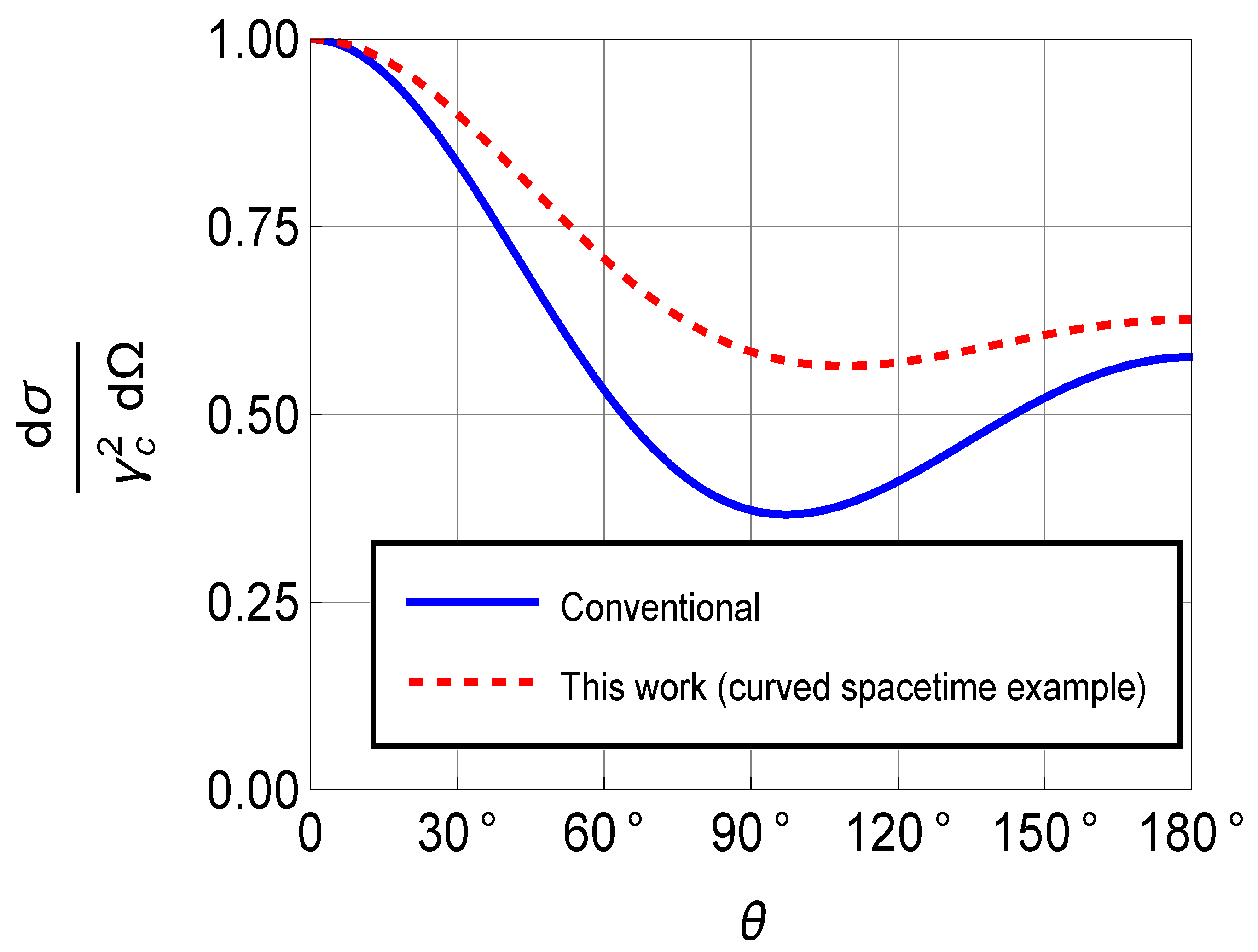
5.2.4. Comparison of Results

For ${\gamma }_{\mathrm{c}}=0.173$, methods A ($4\times 4$) and B ($256\times 256$ in flat spacetime) agree exactly at the algebraic level, confirming that the proposed matrix representation is strictly consistent with the flat-spacetime reference.

Method C (the present $256\times 256$ representation in a curved background) is shown as a toy-model result under the local-constant-metric (LCM) approximation, using constant-coefficient oblique coordinates (including off-diagonal components). As shown in Figure 1, when the coordinate angle $\theta$ is visualized directly, a small deviation appears near $\theta \approx {90}^{\circ }$. This deviation arises because off-diagonal metric components alter the geometric meaning of the coordinate angle; therefore, geometric information associated with the chosen coordinate system is reflected in the plotted angular dependence.

For methods A and B (flat reference), the differential cross section is (Equation (20)):

$${\displaystyle \frac{d\sigma }{d\Omega }}={\displaystyle \frac{0.125\left(1.45043cos\theta -2.40586\left(3+cos2\theta \right)+0.173cos3\theta \right)}{{\left(-1.173+0.173cos\theta \right)}^3}}.$$

(20)

In contrast, method C yields

$$\begin{array}{cc}\hfill {\displaystyle \frac{d\sigma }{d\Omega }}& =5.73001\times {10}^{-20}\left(1.51376\times {10}^{20}-{\displaystyle \frac{3.44859\times {10}^{20}}{1.173-0.173cos\theta }}\right.\hfill \\ \hfill & \left.+{\displaystyle \frac{2.06309\times {10}^{20}}{{(1.173-0.173cos\theta )}^2}}+{\displaystyle \frac{4.62567\times {10}^{18}}{{(1.173-0.173cos\theta )}^3}}\right).\hfill \end{array}$$

(21)

The difference between the flat-spacetime result and the curved-spacetime result (Equation (21)) demonstrates the sensitivity of the framework to metric geometry.

6. Discussion and Limitations

6.1. Focus of the Present Work

The primary purpose of this paper is to internalize the metric $g_{\mu \nu }\left(x\right)$ into matrices and to present an extended Dirac operator

$$D\left(x\right)=i{\widehat{\Gamma }}_{\nu }\left(x\right){\partial }^{\nu }-m,$$

together with matrix- and trace-based calculation rules. Here

$${\widehat{\Gamma }}_{\nu }\left(x\right):=\sum _{\mu =0}^3{\Gamma }_{\mu \nu }\left(x\right),{\Gamma }_{\mu \nu }\left(x\right):={\Gamma }_{\mu }{}^{\rho }{g}_{\rho \nu }\left(x\right),$$

and the basis matrices ${\Gamma }_{\mu }^{\nu }$ are constant $256\times 256$ matrices. In this paper we focus on the definitions and operational rules of this construction, and leave a fully curved treatment (including connection coefficients and full position dependence) as future work.

Note that the indices $\mu ,\nu$ on ${\Gamma }_{\mu }^{\nu }$ are not tensor indices but rather basis labels; ${\Gamma }_{\mu }^{\nu }$ itself is a fixed matrix independent of position (Equation (7)).

6.2. Scope of Applicability

(1)

Consistency in the flat limit: For $g_{\mu \nu }\to {\eta }_{\mu \nu }$, $D\left(x\right)$ matches the standard $4\times 4$ formalism with a unique correspondence via trace normalization. We confirmed exact agreement numerically for tree-level processes (including Compton scattering) [1,7].

(2)

Local-constant-metric (LCM) approximation: When $g_{\mu \nu }\left(x\right)$ varies slowly, one may treat $g_{\mu \nu }$ as approximately constant in a small patch. Under this approximation, $D\left(x\right)$ is operationally useful, and patchwise results can be combined with appropriate weighting to estimate position-dependent effects (the toy models in this paper take this stance).

6.3. Computational Advantages

(1)

The rules are unified in terms of matrix multiplications and traces, which is well suited for automation. Implementations can be shared across processes (effective gammas and spin sums → traces).

(2)

By keeping the trace normalization fixed, one can compare directly against flat reference formulas.

(3)

Parameter scans over metric components are straightforward, enabling reproducible numerical validation.

6.4. Limitations and Future Work

(1)

Loop calculations and renormalization: It remains to be assessed whether the present rules can provide visibility comparable to conventional methods while maintaining a consistent treatment of backgrounds [3,4].

(2)

Position-dependent backgrounds: We plan to implement first-order corrections in perturbative settings (weak gravity, gravitational waves) beyond the LCM approximation and systematically identify processes and scales where deviations could appear.

(3)

Fully covariant derivatives: An extension to a generally covariant form including connection coefficients ${\{}^{\nu }{}_{\rho \sigma }\}\left(x\right)$ is required.

Overall, the present approach is a practical option centered on providing the operator and computational rules. It preserves consistency with flat-spacetime reference formulas and offers rapid, reproducible calculations based on matrix algebra.

7. Conclusions

We defined an extended Dirac operator

$$D\left(x\right)=i{\widehat{\Gamma }}_{\nu }\left(x\right){\partial }^{\nu }-m$$

using a $256\times 256$ two-index gamma-matrix representation in which metric components are internalized on the matrix side. The spacetime dimension remains four; geometric information is encoded as matrix coefficients. We also presented calculation rules that reduce scattering computations to matrix products and traces.

In the flat limit, the framework reproduces standard results with a unique correspondence fixed by trace normalization. We performed trial numerical validations for representative processes (Compton scattering in the main text; Møller scattering, Bhabha scattering, and muon-pair production in the appendices). Within toy models under the local-constant-metric approximation, we showed that off-diagonal metric components can induce characteristic corrections in the angular dependence of scattering cross sections.

A fully curved treatment—i.e., a generally covariant form including connection coefficients ${\{}^{\nu }{}_{\rho \sigma }\}\left(x\right)$,

$$D_{\mathrm{cov}}\left(x\right)=i{\widehat{\Gamma }}_{\nu }\left(x\right)\left({\partial }^{\nu }+{\{}^{\nu }{}_{\rho \sigma }\}\left(x\right)\right)-m,$$

is left as future work.

The advantages of this framework are (i) automation and reproducibility, (ii) direct comparability with flat reference formulas, and (iii) ease of parameter scans over metric components. Future directions include a systematic treatment under an action density including $\sqrt{-g}$, refinement of the anticommutation properties of ${\widehat{\Gamma }}_{\nu }\left(x\right)$, incorporation of first-order corrections in position-dependent backgrounds (weak gravity and gravitational waves), and examination of loop calculations and renormalization.

Appendix B.1. Minkowski Spacetime Calculation with 4×4 γ Matrices

The squared scattering amplitude is given by Equation (A1):

$$\begin{array}{c}\hfill {\left|M\right|}^2={\displaystyle \frac{1}{4}}{\displaystyle \frac{e^4}{q^4}}Tr\left[(\cancel{p}-m){\gamma }^{\mu }(\cancel{p}+m)\right]\\ \hfill ·Tr\left[(\cancel{\kappa }+M){\gamma }^{\mu }(**\kappa *{*}^{\prime }-M){\gamma }_{\nu }\right],\end{array}$$

(A1)

which can be written in terms of Mandelstam variables as (Equation (A2)):

$$\begin{array}{c}\hfill {\left|M\right|}^2={\displaystyle \frac{1}{8m^2{M}^2}}{\displaystyle \frac{e^2}{s^2}}\left[t^2+u^2+4(m^2+M^2)s-2{(m^2+M^2)}^2\right],\end{array}$$

(A2)

where m and M are the electron and muon masses. In the center-of-mass frame at high energy ($s\gg m^2,M^2$), the masses can be neglected and the unpolarized amplitude becomes (Equation (A3)):

$$\begin{array}{c}\hfill {\left|M\right|}^2={\displaystyle \frac{1}{2}}{\displaystyle \frac{e^2}{s^2}}(t^2+u^2).\end{array}$$

(A3)

With the kinematic relations (Equation (A4)):

$$\begin{array}{cc}\hfill t& ={\displaystyle \frac{1}{2}}s(1-cos\theta ),\hfill \\ \hfill u& ={\displaystyle \frac{1}{2}}s(1+cos\theta ),\hfill \end{array}$$

(A4)

and the differential cross section formula (Equation (A5)):

$${\displaystyle \frac{d\overline{\sigma }}{d\Omega }}={\displaystyle \frac{1}{64\pi s}}{\left|M\right|}^2,$$

(A5)

we obtain the final result (Equation (A6)):

$${\displaystyle \frac{d\overline{\sigma }}{d\Omega }}={\displaystyle \frac{1}{4}}{\displaystyle \frac{{\alpha }^2}{s}}(1+{cos}^2\theta ),$$

(A6)

where $\alpha =e^2/4\pi$.

Integrating over the scattering angle yields the total cross section (Equation (A7)) [1]:

$$\begin{array}{cc}\hfill \overline{\sigma }(e^{-}+e^{+}\to {\mu }^{-}+{\mu }^{+})& ={\displaystyle \frac{4\pi {\alpha }^2}{3s}}\hfill \\ \hfill & =1.33333{\displaystyle \frac{\pi {\alpha }^2}{s}}.\hfill \end{array}$$

(A7)

Appendix B.2. Trial Computation in a Curved Background Using Sixteen 256×256 Effective Matrices Γ ^

As in the Compton-scattering computation, we adopt the toy metric:

$$g_{\mu \nu }=\left(\begin{array}{cccc}-1& \frac{1}{20}& \frac{1}{10}& 0\\ \frac{1}{20}& \frac{10}{9}& 0& 0\\ \frac{1}{10}& 0& \frac{10}{9}& 0\\ 0& 0& 0& \frac{10}{9}\end{array}\right).$$

(A8)

We replace all sixteen ${\Gamma }^{\mu }$ used in the computation by $g_{\phantom{\rho }\nu }^{\mu }{\Gamma }^{\nu }$, i.e., we use the effective matrices $\widehat{\Gamma }$ consistent with Equation (A8). A representative result obtained with this choice is given by Equation (A9):

$$\begin{array}{cc}\hfill {\displaystyle \frac{d\overline{\sigma }}{d\Omega }}& ={\displaystyle \frac{8103617490588876123937{\alpha }^2}{30083573867060726457376s}}\hfill \\ \hfill & -{\displaystyle \frac{371011893098098217579{\alpha }^{2}cos\theta }{15041786933530363228688s}}\hfill \\ \hfill & +{\displaystyle \frac{6196145656745290669593{\alpha }^2{cos}^2\theta }{30083573867060726457376s}}.\hfill \end{array}$$

(A9)

Integrating over $\theta$, the total cross section becomes (Equation (A10)):

$$\begin{array}{cc}\hfill \overline{\sigma }(e^{-}+e^{+}\to {\mu }^{-}+{\mu }^{+})& ={\displaystyle \frac{22403380637923042917467\pi {\alpha }^2}{16922010300221658632274s}}\hfill \\ \hfill & \approx 1.32400{\displaystyle \frac{\pi {\alpha }^2}{s}}.\hfill \end{array}$$

(A10)

To visualize the comparison, we plot the results in Figure A1.

Figure A1. Trial example for muon-pair production in $e^{+}{e}^{-}$ collisions.

Figure A1. Trial example for muon-pair production in $e^{+}{e}^{-}$ collisions.

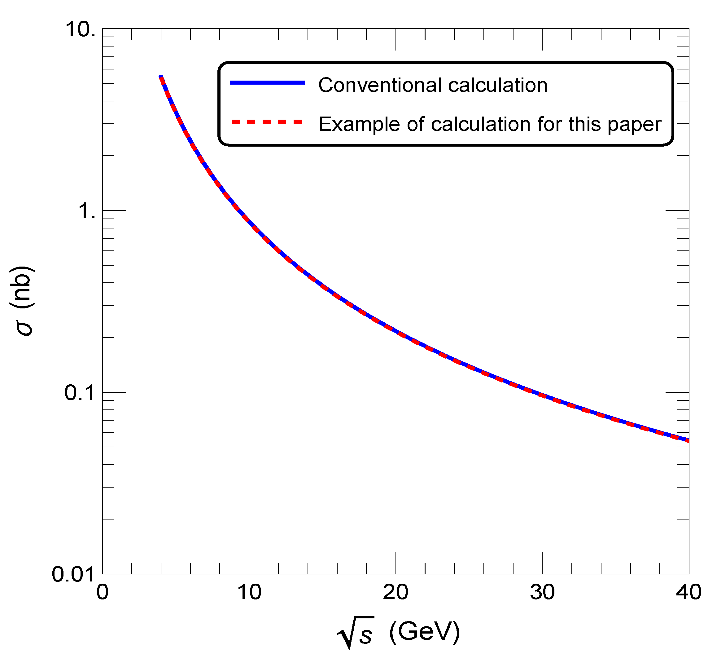
Figure A1 shows that the conventional expression and the present trial result almost overlap. This suggests that this process is relatively insensitive to the chosen toy metric. Therefore, even though $e^{+}{e}^{-}$ collision experiments are feasible at accelerators, testing the present framework with this process would be challenging unless experimental precision is significantly improved.

Appendix C.1. Minkowski-Spacetime Møller Scattering with 4×4 γ Matrices

At lowest order, the Møller-scattering cross section can be written in Mandelstam variables as

$$\begin{array}{cc}\hfill d\sigma & =dt{\displaystyle \frac{4\pi e^4}{{(s-4m^2)}^2}}[f(t,u)+g(t,u)+f(u,t)+g(u,t)],\hfill \end{array}$$

(A11)

with [2] the trace expressions (Equation (A12)):

$$\begin{array}{cc}\hfill f(t,u)& ={\displaystyle \frac{1}{16t^2}}·Tr\left[(**\kappa *{*}^{\prime }+m){\gamma }^{\mu }(\cancel{\kappa }+m){\gamma }^{\nu }\right]\hfill \\ \hfill & ·Tr\left[(**p*{*}^{\prime }+m){\gamma }_{\mu }(\cancel{p}+m){\gamma }_{\nu }\right],\hfill \\ \hfill g(t,u)& =-{\displaystyle \frac{1}{16tu}}·Tr\left[(**\kappa *{*}^{\prime }+m){\gamma }^{\mu }(\cancel{\kappa }+m){\gamma }^{\nu }(**p*{*}^{\prime }+m){\gamma }_{\mu }(\cancel{p}+m){\gamma }_{\nu }\right],\hfill \end{array}$$

(A12)

Substituting into Equation (A11) yields

$$\begin{array}{cc}\hfill f(t,u)& ={\displaystyle \frac{1}{t^2}}\left[{\displaystyle \frac{s^2+u^2}{2}}+4m^2(t-m^2)\right],\hfill \\ \hfill g(t,u)& =g(u,t)={\displaystyle \frac{2}{tu}}\left({\displaystyle \frac{s}{2}}-m^2\right)\left({\displaystyle \frac{s}{2}}-3m^2\right),\hfill \end{array}$$

(A13)

and the cross section becomes (Equation (A14)):

$$\begin{array}{cc}\hfill d\sigma & =r_e^2{\displaystyle \frac{4\pi m^{2}dt}{s(s-4m^2)}}\left\{{\displaystyle \frac{1}{t^2}}\left[{\displaystyle \frac{s^2+u^2}{2}}+4m^2(t-m^2)\right]\right.\hfill \\ \hfill & +{\displaystyle \frac{1}{u^2}}\left[{\displaystyle \frac{s^2+t^2}{2}}+4m^2(u-m^2)\right]\hfill \\ \hfill & \left.+{\displaystyle \frac{4}{tu}}\left({\displaystyle \frac{s}{2}}-m^2\right)\left({\displaystyle \frac{s}{2}}-3m^2\right)\right\},\hfill \end{array}$$

(A14)

where in natural units $r_e=\alpha /m$ so that $r_e^2={\alpha }^2/m^2$.

In the center-of-mass frame, the kinematic relations are (Equation (A15)):

$$\begin{array}{cc}\hfill s& =4{ϵ}^2,t=-4p^2{sin}^2{\displaystyle \frac{\theta }{2}},u=-4p^2{cos}^2{\displaystyle \frac{\theta }{2}},\hfill \\ \hfill -dt& =2p^{2}sin\theta d\theta ={\displaystyle \frac{p^2}{\pi }}d\Omega ,\hfill \end{array}$$

(A15)

where $\left|p\right|$ and $ϵ$ are the electron momentum and energy magnitudes, unchanged by scattering. Substituting and simplifying yields the Møller formula (Equation (A16)):

$$\begin{array}{cc}\hfill d\sigma & =r_e^2{\displaystyle \frac{m^2{({ϵ}^2+p^2)}^2}{4p^4{ϵ}^2}}\left[{\displaystyle \frac{4}{{sin}^4\theta }}-{\displaystyle \frac{3}{{sin}^2\theta }}+{\left({\displaystyle \frac{p^2}{{ϵ}^2+p^2}}\right)}^2\left(1+{\displaystyle \frac{4}{{sin}^2\theta }}\right)\right]d\Omega ,\hfill \end{array}$$

(A16)

which is the Møller-scattering formula.

In the ultrarelativistic limit ($p^2\simeq {ϵ}^2$), the differential cross section becomes [2]

$$\begin{array}{cc}\hfill d\sigma & =r_e^2{\displaystyle \frac{m^2}{{ϵ}^2}}{\displaystyle \frac{1}{4}}{\displaystyle \frac{{(3+{cos}^2\theta )}^2}{{sin}^4\theta }}d\Omega \hfill \\ \hfill & =r_e^2{\displaystyle \frac{m^2}{{ϵ}^2}}{\displaystyle \frac{1}{16}}{(7+cos2\theta )}^2{csc}^4\theta d\Omega ,\hfill \end{array}$$

(A17)

Appendix C.2. Trial Computation in a Curved Background Using Sixteen 256×256 Effective Matrices Γ ^

We present only the ultrarelativistic result ($p^2\simeq {ϵ}^2$); derivation details are provided in Appendix E:

$$\begin{array}{cc}\hfill d\sigma & ={\displaystyle \frac{{\alpha }^2}{71233134002380800000000}}\hfill \\ \hfill & \times (76886835850472311816421\hfill \\ \hfill & +21309289762800530919472cos2\theta \hfill \\ \hfill & +942204894651807977595cos4\theta )\hfill \\ \hfill & \times {csc}^4\theta d\Omega .\hfill \end{array}$$

(A18)

To facilitate comparison between Equations (A17) and (A18), we plot both in Figure A2.

Figure A2. Trial example for the Møller-scattering differential cross section.

Figure A2. Trial example for the Møller-scattering differential cross section.

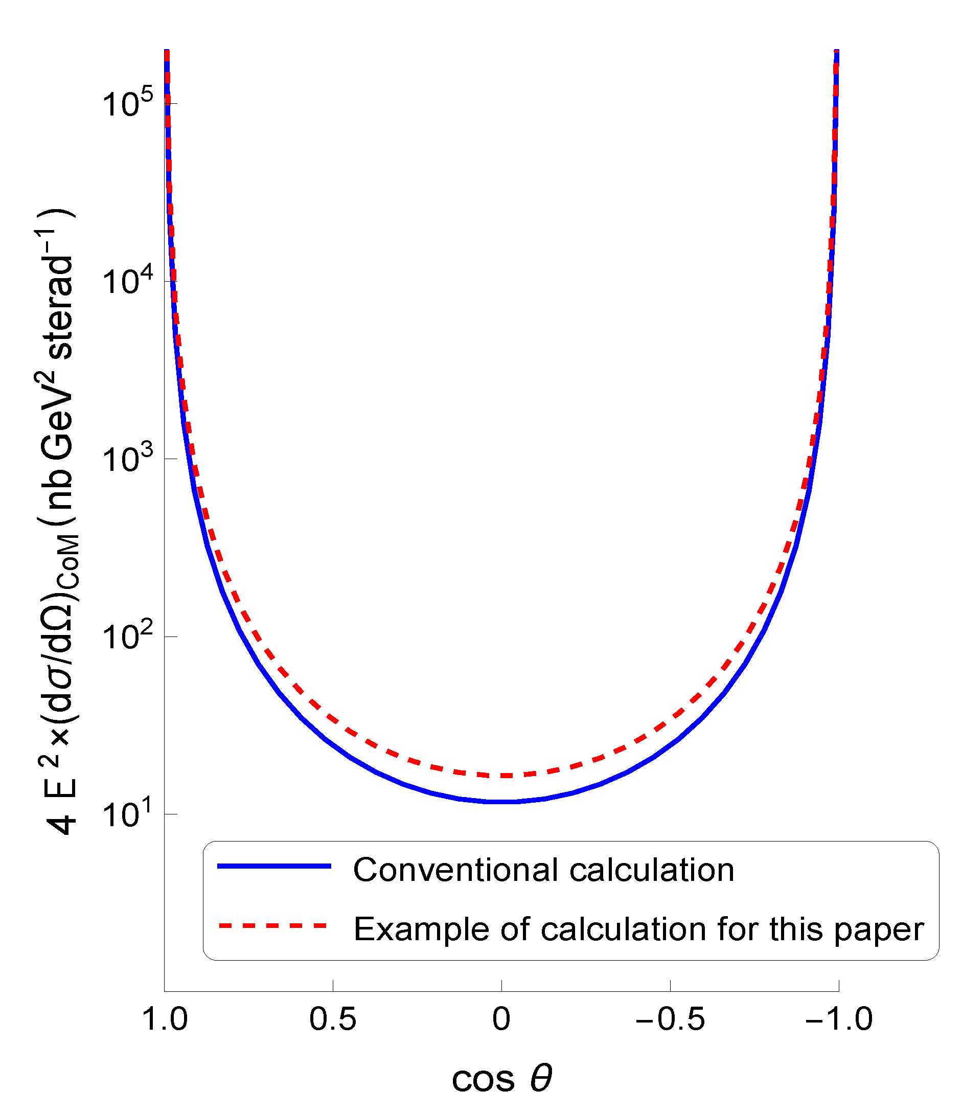
Figure A2 shows that the conventional result (solid blue) and the present trial example (dashed red) differ depending on scattering angle, with the difference becoming more pronounced in the backward region ($cos\theta \to -1$). This indicates that the metric can influence the angular dependence. Experimental verification would require high-precision measurements, but the difference is, in principle, testable.

Appendix D.1. Minkowski-Spacetime Bhabha Scattering with 4×4 γ Matrices

For lowest-order Bhabha scattering, one can obtain the cross section by replacing $s\to u$ in the denominators of the Møller-scattering expressions (Equation (A13)). This yields the Bhabha cross section (Equation (A19)):

$$\begin{array}{cc}\hfill d\sigma & =r_e^2{\displaystyle \frac{4\pi m^{2}dt}{u(u-4m^2)}}\left\{{\displaystyle \frac{1}{t^2}}\left[{\displaystyle \frac{s^2+u^2}{2}}+4m^2(t-m^2)\right]\right.\hfill \\ \hfill & +{\displaystyle \frac{1}{u^2}}\left[{\displaystyle \frac{s^2+t^2}{2}}+4m^2(u-m^2)\right]\hfill \\ \hfill & \left.+{\displaystyle \frac{4}{tu}}\left({\displaystyle \frac{s}{2}}-m^2\right)\left({\displaystyle \frac{s}{2}}-3m^2\right)\right\},\hfill \end{array}$$

(A19)

and in the center-of-mass frame the invariants satisfy (Equation (A20)):

$$\begin{array}{cc}\hfill s& =-4p^2{cos}^2{\displaystyle \frac{\theta }{2}},t=-4p^2{sin}^2{\displaystyle \frac{\theta }{2}},u=4{ϵ}^2,\hfill \end{array}$$

(A20)

where $\left|p\right|$ and $ϵ$ are the electron momentum and energy magnitudes, unchanged by scattering. Substituting and simplifying yields

$$\begin{array}{cc}\hfill d\sigma & =do{\displaystyle \frac{r_e^2}{16}}{\displaystyle \frac{m^2}{{ϵ}^2}}\left\{{\displaystyle \frac{{({ϵ}^2+p^2)}^2}{p^4}}{\displaystyle \frac{1}{{sin}^4\frac{\theta }{2}}}\right.\hfill \\ \hfill & -{\displaystyle \frac{-{ϵ}^4-m^4}{p^2{ϵ}^2}}{\displaystyle \frac{1}{{sin}^2\frac{\theta }{2}}}+{\displaystyle \frac{12{ϵ}^4+m^4}{{ϵ}^4}}\hfill \\ \hfill & \left.-{\displaystyle \frac{4p^2({ϵ}^2+p^2)}{{ϵ}^4}}{sin}^2{\displaystyle \frac{\theta }{2}}+{\displaystyle \frac{4p^4}{{ϵ}^4}}{sin}^4{\displaystyle \frac{\theta }{2}}\right\},\hfill \end{array}$$

(A21)

In the ultrarelativistic limit ($p^2\simeq {ϵ}^2$), the differential cross section simplifies to (Equation (A22)):

$$\begin{array}{cc}\hfill d\sigma & =r_e^2{\displaystyle \frac{m^2}{{ϵ}^2}}{\displaystyle \frac{1}{4}}{\displaystyle \frac{{(3+{cos}^2\theta )}^2}{{sin}^4\theta }}{cos}^4{\displaystyle \frac{\theta }{2}}d\Omega \hfill \\ \hfill & ={\displaystyle \frac{{\alpha }^2}{256{ϵ}^2}}{(7+cos2\theta )}^2{csc}^4{\displaystyle \frac{\theta }{2}}d\Omega \hfill \\ \hfill E_{\mathrm{cm}}^2{\displaystyle \frac{d\sigma }{d\Omega }}& ={\displaystyle \frac{1}{64}}{\alpha }^2{(7+cos2\theta )}^2{csc}^4{\displaystyle \frac{\theta }{2}}.\hfill \end{array}$$

(A22)

Appendix D.2. Trial Computation in a Curved Background Using Sixteen 256×256 Effective Matrices Γ ^

We show only the ultrarelativistic result ($p^2\simeq {ϵ}^2$); details are provided in Appendix E:

$$\begin{array}{cc}\hfill d\sigma & ={\displaystyle \frac{{\alpha }^2}{569865072019046400000000}}\hfill \\ \hfill & \times (678984214898010488151643\hfill \\ \hfill & -85268530601173881371728cos\theta \hfill \\ \hfill & +193781867538668508561356cos2\theta \hfill \\ \hfill & -587053428853200302960cos3\theta \hfill \\ \hfill & +6196145656745290669593cos4\theta )\hfill \\ \hfill & \times {csc}^4{\displaystyle \frac{\theta }{2}}d\Omega .\hfill \end{array}$$

(A23)

To facilitate comparison between Equations (A21) and (A23), we plot both in Figure A3.

Figure A3. Trial example for the Bhabha-scattering differential cross section.

Figure A3. Trial example for the Bhabha-scattering differential cross section.

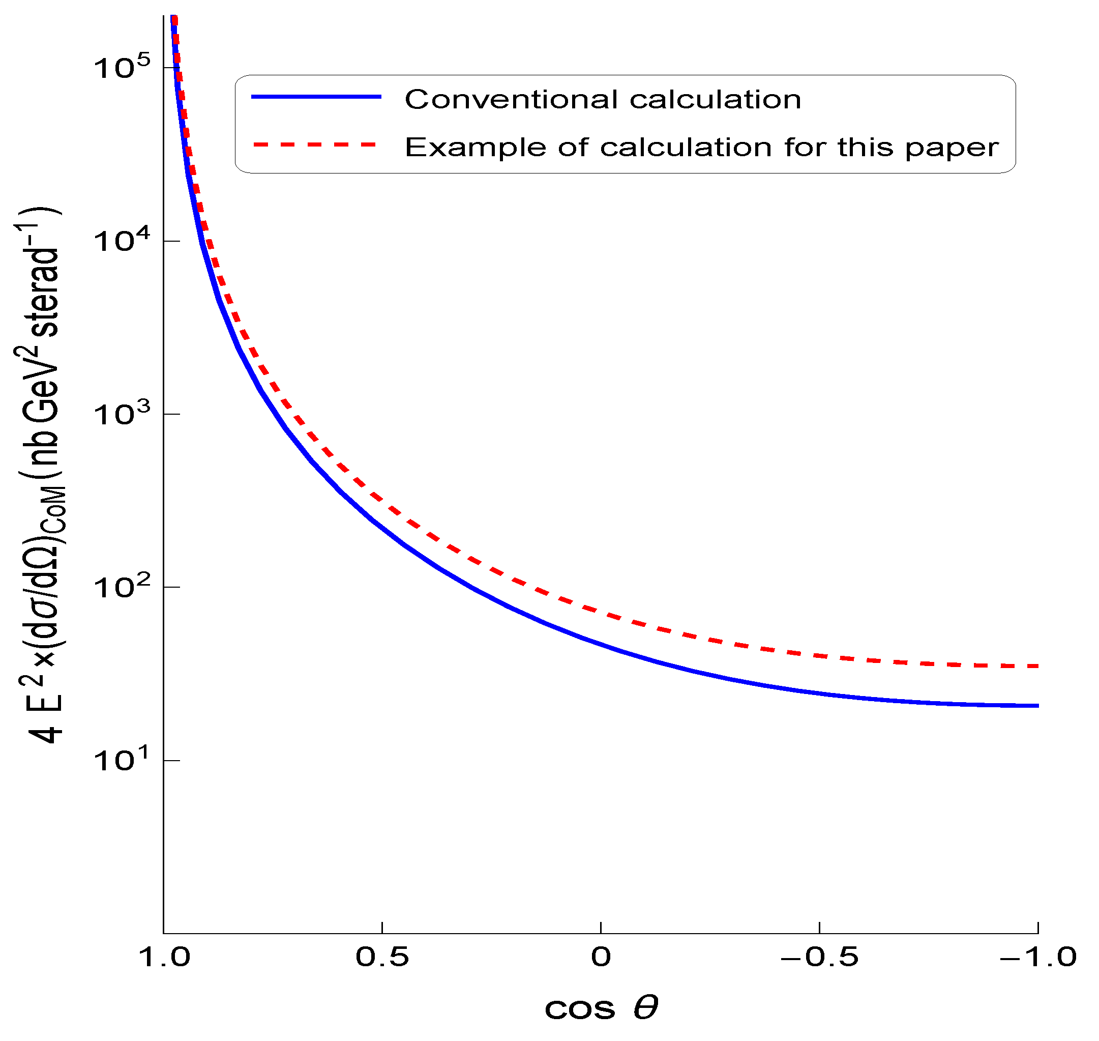
Figure A3 shows angle-dependent differences between the conventional result (solid blue) and the present trial example (dashed red), with the discrepancy tending to be more pronounced in the backward region ($cos\theta \to -1$). This indicates that the metric can influence the angular dependence. Experimental confirmation would require high precision, but the deviation is, in principle, testable.

References

- Peskin, M. E.; Schroeder, D. V. An Introduction to Quantum Field Theory; Addison–Wesley; CRC Press eBook, 1995. [Google Scholar] [CrossRef]
- Berestetskii, V. B.; Lifshitz, E. M.; Pitaevskii, L. P. Quantum Electrodynamics, 2nd ed.; Pergamon (Elsevier), 1982; ISBN 0080265030. [Google Scholar]
- Parker, L.; Toms, D. J. Quantum Field Theory in Curved Spacetime: Quantized Fields and Gravity; Cambridge University Press, 2009. [Google Scholar] [CrossRef]
- Fulling, S. A. Aspects of Quantum Field Theory in Curved Spacetime; Cambridge University Press, 1989. [Google Scholar] [CrossRef]
- Weinberg, S. Gravitation and Cosmology: Principles and Applications of the General Theory of Relativity; Wiley, 1972; ISBN 9780471925675. [Google Scholar]
- Wald, R. M. General Relativity; University of Chicago Press, 1984. [Google Scholar] [CrossRef]
- Klein, O.; Nishina, Y. Über die Streuung von Strahlung durch freie Elektronen nach der neuen relativistischen Quantendynamik von Dirac. Z. Phys. 1929, 52, 853–868. [Google Scholar] [CrossRef]
- Heitler, W. The Quantum Theory of Radiation, 3rd ed.; Oxford University Press; Oxford, 1954. [Google Scholar]
- Bagchi, B.; Ghosh, R.; Gallerati, A. Dirac Equation in Curved Spacetime: The Role of Local Fermi Velocity. Eur. Phys. J. Plus 2023, 138, 1037. [Google Scholar] [CrossRef]
- Arminjon, M.; Reifler, F. Equivalent forms of Dirac equations in curved spacetimes and generalized de Broglie relations. Braz. J. Phys. 2013, 43, 64–77. [Google Scholar] [CrossRef]
- Pollock, M. D. On the Dirac Equation in Curved Space-Time. Acta Phys. Pol. B 2010, 41, 1827–1855. [Google Scholar] [CrossRef]
- Sato, H. Groups and Physics; Maruzen: Tokyo, 1993; ISBN 4621049356. [Google Scholar]
- Lounesto, P. Clifford Algebras and Spinors, 2nd ed.; Cambridge University Press, 2001; ISBN 0521005515. [Google Scholar]
- Lawson, H. B., Jr.; Michelsohn, M.-L. Spin Geometry; Princeton University Press, 1989; ISBN 9780691085425. [Google Scholar]
- Porteous, I. R. Clifford Algebras and the Classical Groups; Cambridge University Press, 1995; ISSN ISBN: 0521551778. [Google Scholar]
- Hestenes, D. Clifford Algebra to Geometric Calculus: A Unified Language for Mathematics and Physics; Reidel (Kluwer), 1984; ISSN ISBN: 9027715666. [Google Scholar]
- Doran, C.; Lasenby, A. Geometric Algebra for Physicists; Cambridge University Press, 2003; ISBN 0521715954. [Google Scholar]
- Shapiro, I. L. Covariant Derivative of Fermions and All That. Universe 2022, 8(11), 586. [Google Scholar] [CrossRef]
Figure 1.
Comparison of computational methods for Compton scattering (). Methods A and B (flat spacetime; and ) coincide exactly and serve as a validation benchmark. Method C shows a toy-model result using constant-coefficient oblique coordinates (including off-diagonal components) within the local-constant-metric (LCM) approximation. This figure is intended as a demonstration of (i) correct operation of the proposed matrix-based computation rules and (ii) sensitivity to coordinate choice; it does not claim a direct physical curvature-induced effect.
Disclaimer/Publisher’s Note: The statements, opinions and data contained in all publications are solely those of the individual author(s) and contributor(s) and not of MDPI and/or the editor(s). MDPI and/or the editor(s) disclaim responsibility for any injury to people or property resulting from any ideas, methods, instructions or products referred to in the content. |
© 2026 by the authors. Licensee MDPI, Basel, Switzerland. This article is an open access article distributed under the terms and conditions of the Creative Commons Attribution (CC BY) license (http://creativecommons.org/licenses/by/4.0/).
Copyright: This open access article is published under a Creative Commons CC BY 4.0 license, which permit the free download, distribution, and reuse, provided that the author and preprint are cited in any reuse.