Submitted:
13 October 2025
Posted:
14 October 2025
You are already at the latest version
Abstract
We present a unified geometric framework for the full Lorentz group, based on a bounded angle parametrization of spacetime transformations within a hyper-spherical geometry. By mapping the unbounded hyperbolic angle φ to a bounded angle β using the Gudermannian function, hyperbolic, causal, and Euclidean three-spheres are brought together into a single structure: hyper-spacetime. This structure unifies the Euclidean R4 and Minkowski R1,3 domains, incorporates discrete symmetries in a continuous way, and removes discontinuities at the lightlike boundary. Each three-sphere carries a natural spinor set, encoding symmetry, and acting as eigen-spinors of corresponding observables. These reproduce the Dirac spectrum while confining singular behavior to a scalar factor. The bounded angle parametrization therefore provides a continuous, closed representation of the full Lorentz group and a transparent geometric basis for spacetime symmetry.
Keywords:
full Lorentz group
; spacetime spinors
; three-sphere
; hyper-spacetime
; geometric algebra
; Dirac equation
; null spinors
; geometric duality
1. Introduction
The full Lorentz group [1,2,3,4,5,6] encodes the fundamental symmetries of spacetime. It includes both continuous transformations - boosts and spatial rotations - as well as discrete reflections. Conventionally, Lorentz boosts are parameterized by the unbounded angle (rapidity). While effective, this parametrization leads to discontinuities at the lightlike boundary, and leaves the discrete symmetries disconnected from identity.
In this paper, we introduce a bounded representation of the full Lorentz group by embedding its transformations into a closed hyper-spherical geometry, which we term hyper-spacetime. The main step is to map the unbounded angle to a bounded angle using the Gudermannian function [7,8]. This mapping enables smooth passage across infinity, incorporates discrete transformations in a continuous manner, and eliminates algebraic singularities at the lightlike boundary.
The core of the paper (Section 2, Section 3, Section 4, Section 5 and Section 6) develops the mathematical framework. We first reformulate Lorentz boosts using a bounded angle parametrization that unifies circular and hyperbolic symmetry and applies naturally to special relativity, yielding harmonic relativistic proportionality factors [9]. Extending to four dimensions, we introduce a triplet of three-spheres that define hyper-spacetime and show how the full Lorentz group, with both continuous and discrete symmetries, emerges within its hyper-spherical coordinates. Spinor sets are then constructed and analyzed as eigen-spinors of geometric observables, reproducing the Dirac spectrum while confining singularities to scalar factors. The final part of the paper (Section 7 and Section 8) turns to interpretation and outlook, discussing the physical implications of hyper-spacetime, and concludes with a summary of its unifying features.
The mathematical formalism throughout is based on the geometric algebra (GA) of spacetime (STA) as developed by David Hestenes [10,11] (Appendix A). Foundations of geometric algebra where laid by Grassmann [12] and Clifford [13] in the 19th century, and the decisive motivation for its use lies in the generalization of rotations via rotors [14,15,16,17,18]. In STA [10], a spacetime inertial frame is represented by four orthogonal basis vectors , which satisfy the algebra of the Dirac gamma matrices [4].
2. Hyperbolic Rotation
Lorentz boosts are conventionally expressed as hyperbolic rotations, parameterized by the unbounded angle (rapidity) (Figure 1a).
A boost along the -axis (-axis) is generated by the hyperbolic rotor :
Where bivector represents the temporal plane of rotation. Acting on the temporal basis vector , the rotor generates the boosted spacetime vector :
However, rotor only covers the positive branch of the hyperbola. The negative branch of the hyperbola is not present (Figure 1a).
To cover the full hyperbolic symmetry in a single parameter domain, we map the unbounded angle onto the bounded angle using the Gudermannian function (Appendix B) [7,8]. Substituting of this function into yields the rotor :
The scalar factor ensures normalization, while acts as a temporal spinor (Appendix C). Applying rotor to generates the boosted spacetime vector :
Where the full hyperbolic symmetry is covered continuously (Figure 1b).
In summary, the bounded angle parametrization provides several advantages. It removes singularities by isolating them in the scalar density factor , while the associated spinor remains regular. At , the mapping passes smoothly through infinity, ensuring continuity across the lightlike boundary where crossing corresponds to a time reversal. The two disconnected hyperbolic branches and are thereby closed into a single hyperbolic one-sphere (Figure 1b). In this way, hyperbolic symmetry is unified within a single angular cycle.
3. Harmonic Relativistic Proportionality Factors
In special relativity, the relative speed is conventionally mapped to the unbounded angle (rapidity). Using instead the bounded angle introduced in Section 2, this mapping provides a harmonic set of relativistic proportionality factors:
These factors form a bridge between circular and hyperbolic symmetry:
Consequently, the bounded angle mapping unifies circular with hyperbolic symmetry (Figure 1b). A complete cycle on one-sphere corresponds one-to-one with a complete cycle on hyperbolic one-sphere . This includes a smooth passage through infinity at the lightlike boundaries .
To incorporate all the symmetries of the full Lorentz group , the framework must extend from the two-dimensional (2D) relation to a four-dimensional (4D) relation that unifies the Euclidean domain with the Minkowski domain .
4. One Unified Geometry Bridging
and
The generalization from two to four dimensions is realized by the introduction of a triplet of three-spheres embedded in a Euclidean and a Minkowski domain (Appendix A). We define three distinct but related three-spheres:
Here:
• The hyperbolic three-sphere is preserved by spacetime rotor (Figure 2b).
• The causal three-sphere is preserved by spacetime spinor (Figure 3a).
• The Euclidean three-sphere is preserved by Euclidean spinor (Figure 3b).
Each of these three-spheres is preserved by a specific spinor structure (as defined in section 4.1), which ensures that the geometry remains invariant under both Lorentzian and Euclidean transformations. In this way, every three-sphere is not only defined by its metric but also carries a natural spinor representation that encodes its symmetry.
All three-spheres share: a common temporal axis , a common origin (spacetime event), and a common temporal bivector plane. They differ in their metric and spatial subspaces and (Eq. 7), which define two complementary two-spheres:
Both two-spheres are preserved by spatial spinor (Figure 2a):
They are orthogonal to , aligned , and define spatial direction. Moreover, they span a common temporal bivector plane , which is a cornerstone of the unified geometry. The Minkowski vectors thus reappear in the Euclidean domain as temporal bivectors, while the Euclidean vectors play the same role in the Minkowski domain. This geometrical duality: specifies spatial direction while simultaneously encoding for temporal orientation in the opposite domain. Their associated dual spatial bivector planes belongs to the common three-dimensional even subalgebra (Appendix A), ensuring domain-independence of spatial orientation.
4.1. Definition of the Spinors
, Rotor , and Vectors , and associated rotor , form a spinor structure that preserves the triplet of three-spheres (Figure 2 and Figure 3). Thus, every three-sphere carries a natural spinor representation that encodes its symmetry. The Euclidean spinor (preserving ) and spacetime spinor (preserving and ) are defined as:
Here acts as a spatial spinor (Eq. 9), and act as temporal spinors (Appendix C), and the scalar factor ensures the unitarity of rotor , the normalized form of . Applying the spinors and yields the vectors spanning the three-spheres:
Here, is a hyperbolic unit vector, is a causal vector with variable norm, and is a Euclidean unit vector. The causal three-sphere covers the spacetime region bounded by the light cone of a past event (Figure 3a). Each vector is future pointing and its norm represents proper length, vanishing at the lightlike boundaries. In this way, integrates a natural form of causality in the triplet of three-spheres.
In summary, the three-spheres (Eq. 7) exhibit the following features:
• A common temporal axis with a shared origin (spacetime event).
• Unit vectors and that encode spatial direction and temporal orientation through the dual relation , expressing a geometric duality between domains.
• Domain-independent spatial bivector planes , common to both domains.
A complete cycle on the Euclidean three-sphere corresponds one-to-one with a complete cycle on hyperbolic three-sphere , thereby unifying and . The apparent boundary at infinity () is absorbed smoothly, making the entire structure closed and traversable. We therefore define the unified geometry constructed from the triplet of three-spheres as hyper-spacetime :
Its coordinates are given by the hyper-spherical set , where the spatial angles encodes direction and the temporal angle encodes relative speed (Eq. 5). Hence, the familiar relativistic parameters of direction and speed are reformulated as angular variables in a closed domain, and continuity at the lightlike boundaries.
5. Full Lorentz Group
The full Lorentz group [19,20,21] contains the symmetries of spacetime that preserve the Minkowski metric. It includes: 1) continuous transformations as boosts and spatial rotations, and 2) spacetime event reflections : identity (I), parity (P), time-reversal (T), and spacetime-reversal (PT). Thus, the full Lorentz group is defined as:
where is the proper orthochronous Lorentz subgroup connected to identity.
In the conventional formalism: boosts in are parameterized by the unbounded angle , leading to singularities at the lightlike boundaries. Moreover, the discrete reflections remain disconnected from identity. The standard way to extend the full Lorentz group is through its double cover , as it includes both proper and improper transformations [21]. However, even within , the discrete transformations remain disconnected from identity, leaving a gap between reflections and continuous transformations. This gap is closed by hyper-spacetime, in which continuous and discrete symmetries arise naturally within a unified geometry.
5.1. A Unified Geometry
In the hyper-spherical coordinates of hyper-spacetime (defined in Section 4), the spacetime event reflections manifest naturally as smooth angular transformations:
These transformations correspond to changes in temporal orientation (sign changes or shifts in ) and spatial orientation ( shifts in ). Crucially, all four reflections are smoothly connected to identity, eliminating discontinuities.
5.2. Spinor Representations
The spinor structure of hyper-spacetime provides explicit representations of the transformations. Starting from the spacetime spinor , variations in the hyper-spherical coordinates generate the full set of spacetime spinors , where each of the spinors represents one of the transformations:
With . Similarly, changes in generate the full set of Euclidean spinors :
With . Note the algebraic closure: each of the spinors and can be a basis to generate the full set of transformations. The spatial spinors in and are generated from spatial spinor (Figure 2a) via a parity transformation:
This orthonormal set corresponds to the spatial Pauli spinors [22].
Each set and forms an orthonormal basis within its respective metric, and the discrete transformations remain continuously connected to identity. The components of both sets are identical, differing only in their temporal bivector plane: in the Minkowski domain versus in the Euclidean domain.
In summary, hyper-spacetime provides:
• A smooth, closed, continuous angular domain for the full Lorentz group .
• Discrete reflections , continuously connected to identity.
• Spinor sets forming orthonormal bases in their respective metrics, unifying the Euclidean domain with the Minkowski domain .
• A closed realization of the double cover through the spinor sets .
• Isolation of infinities at the lightlike boundaries into the scalar density factor (Eq. 11), while the spinors themselves remain regular.
This prepares the ground for Section 6, where the eigen-spinor and eigenvalue structure of physical observables in hyper-spacetime is developed.
6. Eigen-Spinors and Eigenvalues in the Geometry of Hyper-Spacetime
Analogous to how the observables of lie on the surface of the one-sphere , the observables of hyper-spacetime reside on the surfaces of the three-spheres , each preserved by the spinor sets . These spinor sets act not only as symmetry generators, but also as eigen-spinors of the corresponding observables (Eq. 12). This follows directly from the geometric algebra eigen-spinor eigenvalue relation (Appendix D):
Here, is an observable, is a basis vector (reference observable, e.g., ), are the eigen-spinors of , and the corresponding eigenvalues. In hyper-spacetime, however, the spinor sets are generated geometrically by variations in the hyper-spherical coordinates (Eq. 15), rather than being obtained by solving an eigen-spinor eigenvalue equation explicitly (Appendix D).
6.1. Spatial Eigen-Spinors
The spatial spinor set (Eq. 18), generated from a parity transformation, act as eigen-spinors of the spatial unit vectors (Figure 2a) and (Eq. 10). They satisfy the GA eigen-spinor eigenvalue relations (Appendix D):
So, and are observables with eigen-spinors and eigenvalues . Physically, these correspond to spin-up or spin-down measurements along the spatial directions of and .
6.2. Spacetime Eigen-Spinors
The spacetime spinor set (Eq. 16) and Euclidean spinor set (Eq. 17) act as eigen-spinors of the hyper-spacetime observables (Eq. 12):
Here, the eigenvalues encodes two constant spin states combined with positive/negative temporal orientation in and , while the eigenvalues encodes two variable spin states combined with positive/negative temporal orientation in . Unlike , the values of depend on relative speed via angle (Eq. 5). Hence, a spin state in vanishes at the lightlike boundaries .
6.3. Null Spinors
At the lightlike boundaries (), the spacetime spinors reduce to null spinors:
These spinors have zero intensity but preserve direction, lying on the light cone of and . For the Euclidean spinors , the corresponding boundary form is:
Thus, the Euclidean spinors keep their unit intensity, while the intensities of spacetime spinors become zero. Each spinor set pass smoothly through the lightlike boundary.
6.4. Correspondence with the Dirac Equation
The eigen-spinors (Eq. 21) and eigenvalues of the observable reproduce those of the Dirac equation [14] (two spin states combined with positive/negative temporal orientation, i.e., matter/antimatter) (Appendix E). This agreement is remarkable, because in hyper-spacetime these eigen-spinors are generated geometrically (Eq. 16), rather than being obtained by solving an eigen-spinor eigenvalue equation (Appendix D). This establishes a direct geometric origin for the Dirac spectrum, demonstrating that the fundamental structure of spacetime eigen-spinors emerges naturally within the hyper-spacetime framework.
In summary, the eigen-spinor structure of hyper-spacetime reproduces the Dirac spectrum, isolates singularities into a scalar density, and reveals null spinors as natural lightlike states.
7. Discussion
The unified hyper-spacetime framework extends the full Lorentz group into a continuous, bounded, and closed representation that reproduces the Dirac eigen-spinor spectrum while exposing structural features obscured in conventional formulations.
The agreement between Dirac eigen-spinors and the spinors of hyper-spacetime is striking: whereas Dirac spinors encode intrinsic particle properties, in hyper-spacetime they emerge directly from geometry through variations in the hyper-spherical coordinates (Eq. 15). This correspondence shows that the algebraic structure of the Dirac equation can be understood as a geometric property.
In hyper-spacetime, boosts and spatial rotations combine seamlessly with the discrete symmetries , which appear as smooth angular transformations in the closed domain of . The replacement of the unbounded rapidity by the bounded angle closes the hyperbola , incorporating the lightlike boundaries as regular points. This generalizes naturally to the four-dimensional (4D) hyperbolic three-sphere , where infinities are absorbed into a smooth boundary.
The causal three-sphere covers the spacetime region bounded by the light cone of a past event, a four-dimensional causality volume containing all information accessible to observation (Figure 3a). It is spanned by future-pointing vectors of variable norm . The Euclidean three-sphere , with its positive-definite metric, ensures completeness. Together, the three-spheres share a common temporal axis , origin (spacetime event), and temporal bivector plane (Eq. 10). This bivector plane expresses the geometric duality of the aligned spatial vectors, as and act as vector bivector counterparts in opposite domains. They are linking spatial direction with temporal orientation and thereby unifying the Euclidean and Minkowski domains. Hyper-spacetime thus provides a natural setting for Wick rotations and periodic time in path integrals [23,24], without the need to introduce imaginary time.
A direct manifestation of this duality is the emergence of temporal spinors (Appendix C). Both spacetime spinors and the Euclidean spinors decompose into spatial and temporal spinors (Eq. 16, 17). The spatial spinors encode orientation in the spatial bivector plane , which lies in the common three-dimensional even subalgebra and is domain-independent, while the temporal spinors encode orientation in the shared temporal bivector plane. In this way, the spinor decomposition mirrors the dual geometric structure of hyper-spacetime.
The physical status of hyper-spacetime must ultimately be tested experimentally. We therefore challenge experimentalists [25,26] to search for phenomena that could reveal the predicted link between particle properties and spacetime geometry. Such confirmation would show that hyper-spacetime is not only mathematically consistent but also offers a new perspective on nature. This article has focused on establishing hyper-spacetime as a consistent framework: a closed representation of the full Lorentz group enriched by new geometric elements - temporal spinors, null spinors, and a shared bivector plane - that provide a foundation for future work.
8. Conclusion
The hyper-spacetime framework provides a bounded, continuous, and closed representation of the full Lorentz group . Through a unified three-sphere geometry and hyper-spherical coordinates , it removes discontinuities, incorporates both continuous and discrete transformations in a single smooth domain, and reproduces the Dirac eigen-spinor spectrum with singularities isolated in scalar factors. Beyond these established results, hyper-spacetime introduces new elements - temporal spinors, null spinors, and a shared bivector plane - that offer a fresh perspective on spacetime symmetry. Together, these features define a consistent framework and a foundation for future exploration of geometric structure in nature.
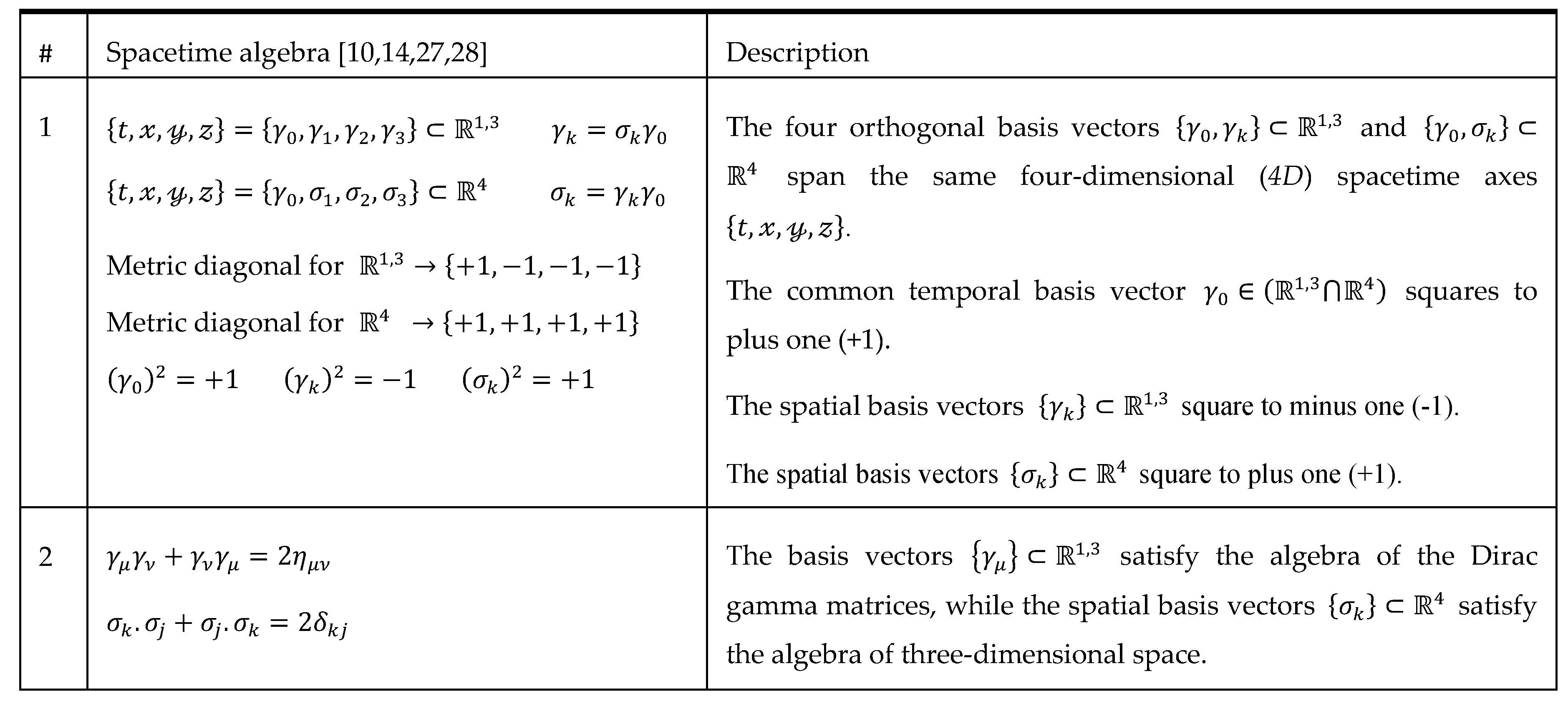
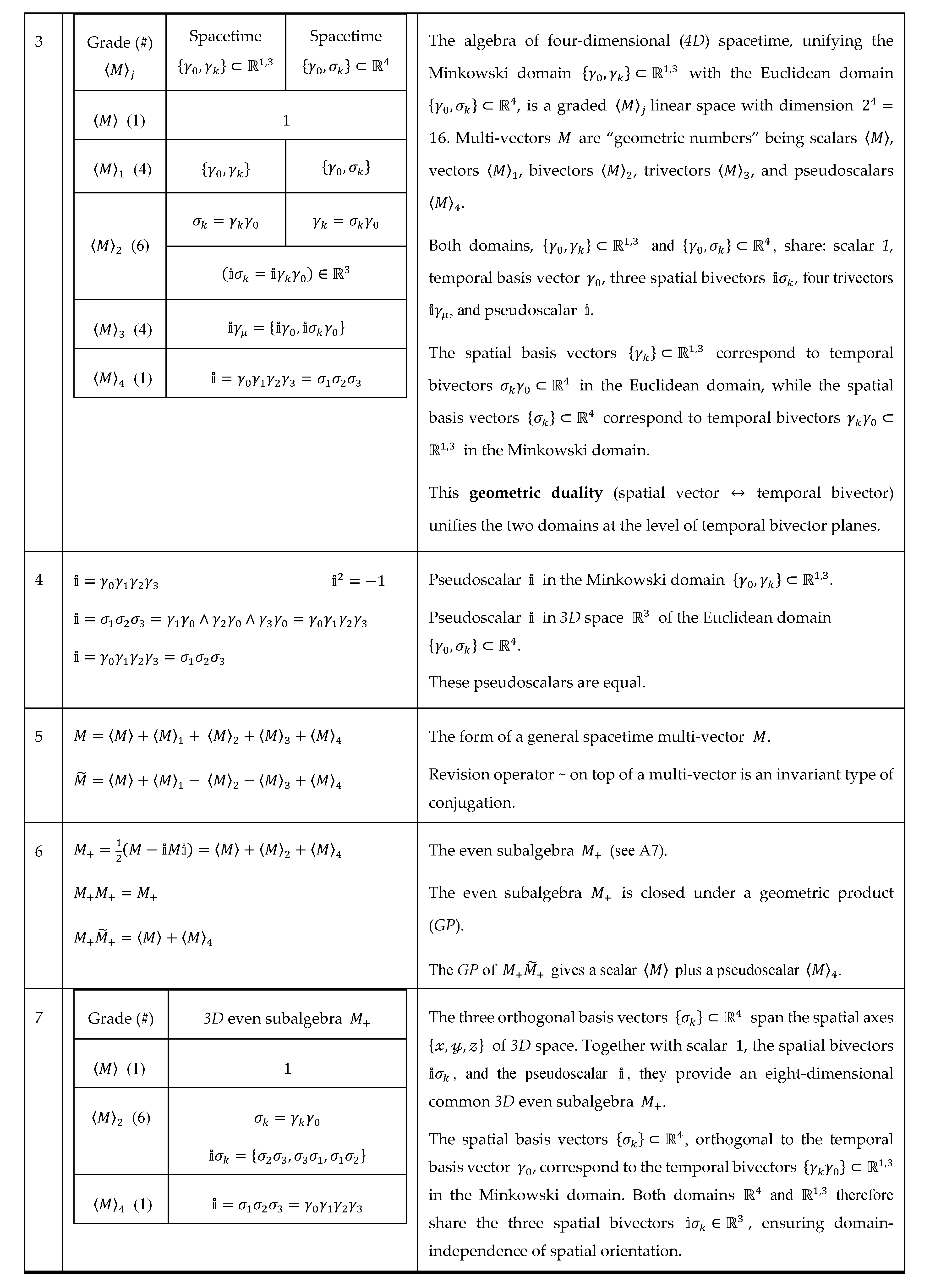
Appendix A: Spacetime Algebra

Table A1.
Spacetime algebra bridging and
|
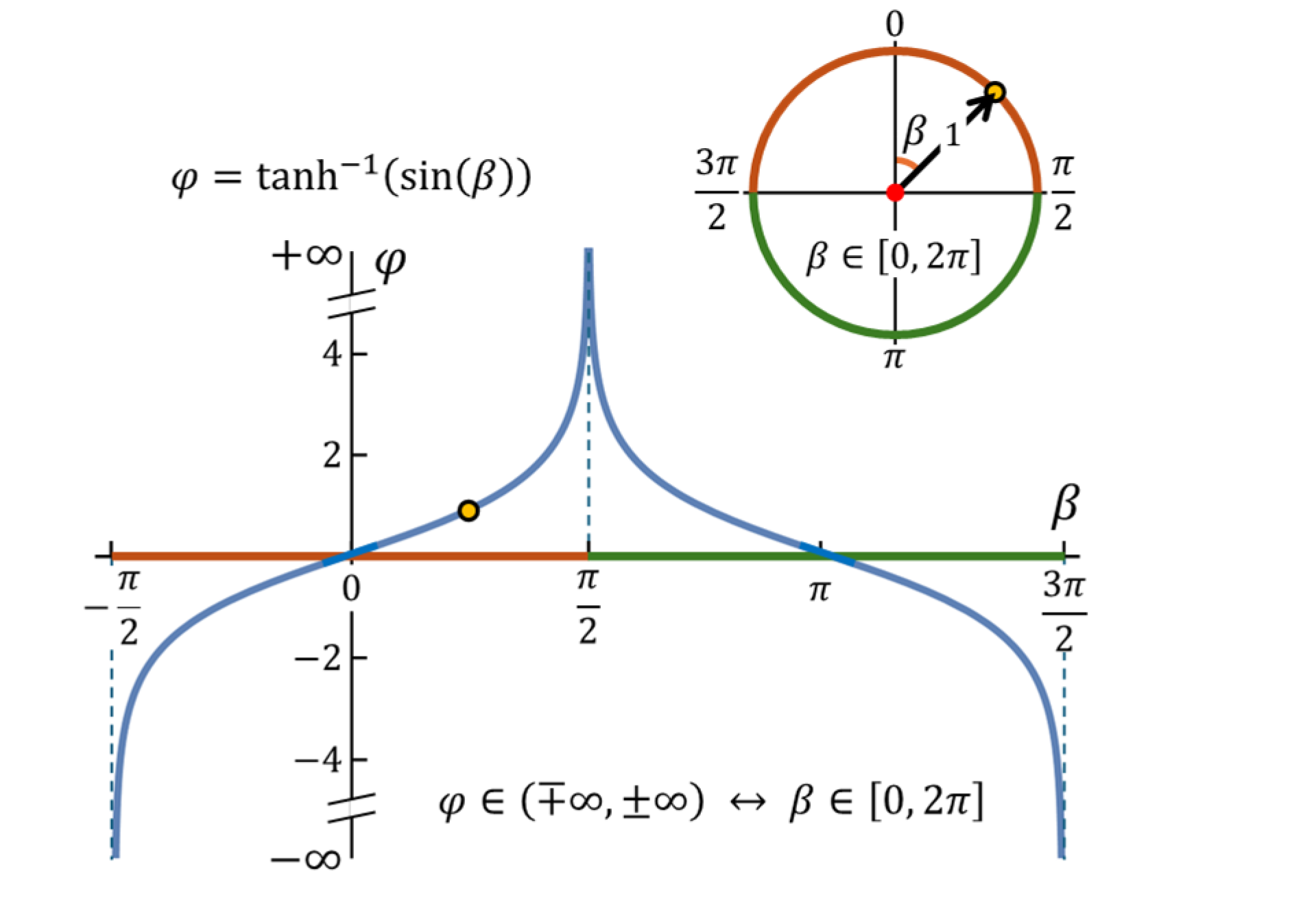
Appendix B: Gudermannian Function
The Gudermannian* function [7,8]:
relates the unbounded hyperbolic angle to the bounded and periodic angle (Figure B1).
Figure B1.
The Gudermannian function provides a smooth mapping between the unbounded angle and the bounded angle .
Figure B1.
The Gudermannian function provides a smooth mapping between the unbounded angle and the bounded angle .
A hyperbolic unit vector spans the two separate branches of a hyperbola.
Substitution of the Gudermannian function into eliminates the need to treat the two branches separately, yielding a single smooth parametrization:
Consequently, the full hyperbola is covered in one continuous domain, including the points at infinity (), which appear as regular boundary points.
The choice of the Gudermannian function is not arbitrary. It establishes a direct one-to-one correspondence between trigonometric and hyperbolic functions without introducing complex arguments. The Gudermannian function in its primary form maps unbounded angle to the bounded angle interval , where the hyperbolic functions are positive. To extend this mapping to the full periodic domain , one must also include the negative hyperbolic functions, which correspond to a shift of the trigonometric functions. This yields the following Gudermannian functions:
Together, the positive and negative branches cover the full periodic domain (Figure B1). So, the Gudermannian function unifies circular and hyperbolic symmetry, ensuring that both boosts and rotations are treated within a single angular domain.
* Christoph Gudermann (25 March 1798 – 25 September 1852) introduced this function and the concept of uniform convergence. See Wikipedia.
Appendix C: Spinors and Rotors
In geometrical algebra (GA) the rotation of a multivector by a rotor is performed by a double-sided geometric product (GP):
This is a powerful generalization of rotation, as it applies in any dimension and to any multivector. A rotor can be written as a scalar density times a spinor :
Here the unitarity of the rotor determines the scalar density . In general, for a spinor to define a proper rotor, its intensity must be a scalar:
Any nonzero additional grade contribution to the intensity would prevent normalization with a scalar density (Eq. C2).
A spinor is characterized by its bivector, i.e., the plane of rotation. In hyper-spacetime the Minkowski domain and the Euclidean domain share the three spatial bivectors (Appendix A). Hence a general spatial spinor is:
The three temporal bivectors in the Minkowski domain are . Hence, a general Minkowski temporal spinor is:
The three temporal bivectors in the Euclidean domain are . Hence, a general Euclidean temporal spinor is:
Both the spatial and the two temporal spinors are pure spinors, since their intensities reduce to scalar values.
The pure spinors (Eq. 16, 17) preserving hyper-spacetime and acting as eigen-spinors, are geometrically generated from the spinors and (Eq. 11). Both are composed of a spatial spinor (Eq. 9) and the temporal spinors and :
The associated proper rotor , the normalized form of , is:
The rotor associated with spinor is equal to , since its intensity satisfies . The same holds for the spatial spinor , which also has unit intensity.
The temporal spinors and (Eq. C7), characterized by the temporal bivectors and , reveal the dual role of these temporal bivector planes across hyper-spacetime . In this dual relation, the temporal bivectors of the Euclidean domain appear as the spatial basis vectors of the Minkowski domain, while the temporal bivectors of the Minkowski domain play the same role in the Euclidean domain. This geometric duality unifies the two domains at the level of their temporal bivector planes. Moreover, the two domains share the three spatial bivectors (Eq. C4), which belong to a common three-dimensional even subalgebra, ensuring that the spatial spinors remain domain-independent.
Appendix D: Eigen-Spinors and Eigenvalues
The hyper-spacetime spinor sets (Eq. 16, 17), which preserve the three-spheres , act also as eigen-spinors of the corresponding observables . Their connection is described by the geometric algebra eigen-spinor eigenvalue relation:
Here, is a observable, is a basis vector (reference observable, e.g., ), is the eigen-spinor set of , and the eigenvalues of . However, in hyper-spacetime these spinor sets are geometrically generated (Eq. 16, 17), rather than being obtained by solving an eigen-spinor eigenvalue equation.
To calculate eigen-spinors and eigenvalues in practice, one uses the linear algebra (LA) eigen-spinor eigenvalue equation:
where is the matrix representation of the observable, the column vector representation of the eigen-spinors, and the eigenvalues. A one-to-one conversion between GA and LA is obtained via the standard matrix representations of the basis vectors:
Using these, the observables become 4 by 4 matrices:
where is the 2 by 2 spatial spin observable matrix associated with the spatial unit vectors and (Eq. 10):
Solving the LA eigen-spinor eigenvalue equation (D2) for gives the spatial eigen-spinors with eigenvalues :
Here, the set are the orthonormal spatial Pauli spinors [22]. Similarly, solving equation (D2) for the observables yields the column vector eigen-spinor sets:
with eigenvalues and .
In summary, the eigen-spinors and (D7) obtained by solving the LA eigen-spinor eigenvalue equation are equal to the geometrically generated (Eq. 15) spacetime spinor sets (Eq. 16, 17).
Appendix E: Dirac Equation
This appendix provides the explicit correspondence between 1) the spacetime spinors obtained as solutions of the Dirac equation and 2) the geometrically generated spacetime spinors (Eq. 16).
The observables , as elements of the three-spheres , are normalized vectors and can directly be linked to relativistic dynamics. The hyperbolic three-sphere vector corresponds to normalized momentum:
While the causal three-sphere vector corresponds to normalized distance:
The geometric product of and yields relativistic action [29]:
Treating action as a phase , a free particle plane-wave state [14] is defined as:
Where, is the normalized action, and is a constant spacetime spinor. This plane-wave state is a solution of the Dirac equation in geometric algebra [14]:
which is equivalent to the linear algebra (LA) form [4]:
Substitution of the plane wave state in (Eq. E5) shows that spinor satisfies the GA eigen-spinor eigenvalue relation:
Multiplying from the right with gives:
Hence, plane wave state (Eq. E4) is a solution of the Dirac equation.
Finally, variations in the hyper-spherical coordinates of , encoded by the spacetime event reflections (Eq. 15), generate the four Dirac plane-wave solutions:
The orientation of action depends on the temporal angle , such that matter and antimatter solutions follow naturally from the spacetime event reflections . Each of these plane-waves is a valid solution of the Dirac equation, demonstrating the remarkable correspondence between the Dirac equation and the spacetime event reflections .
In addition to the four fermionic Dirac plane-wave solutions , these solutions also yield a lightlike boundary solution at :
This corresponds to a photon-like state with vanishing mass term. At the lightlike boundary, the fermionic plane-wave solutions reduce to null spinors with zero intensity while retaining directionality. Thus, the hyper-spacetime framework produces both fermionic (massive) and photonic (massless) solutions as limiting cases of a unified spinor structure.
References
- Vaughan-Hankinson, B. , 1 The Lorentz Group. 2019.
- Gray, J. , Henri Poincaré, in Henri Poincaré. 2012, Princeton University Press.
- Schwichtenberg, J. , Physics from symmetry. 2018: Springer.
- Thomson, M. , Modern particle physics. 2013: Cambridge University Press.
- Bonolis, L. , From the rise of the group concept to the stormy onset of group theory in the new quantum mechanics: A saga of the invariant characterization of physical objects, events and theories. La Rivista del Nuovo Cimento, 2004. 27(4-5): p. 1-110.
- Cao, T.Y. , Conceptual development of 20th century field theories. 2019: Cambridge University Press.
- Gambini, A., G. Nicoletti, and D. Ritelli, A Structural Approach to Gudermannian Functions. Results in Mathematics, 2024. 79(1): p. 10.
- Gudermann, C. , Theorie der Modular-Functionen und der Modular-Integrale. Journal für die reine und angewandte Mathematik (Crelles Journal), 1838. 1838(18): p. 1-54.
- Brands, P.J. , Hyperbolic Rotation with Euclidean Angle Illuminates Spacetime Spinors. J Math Tech-niques Comput Math, 2023. 2(11): p. 456-478.
- Hestenes, D. , Space-time algebra. 2015: Springer.
- Hestenes, D. , Spacetime physics with geometric algebra. American Journal of Physics, 2003. 71(7): p. 691-714.
- Grassmann, H. , A New Branch of Mathematics: The "Ausdehnungslehre" of 1844 and Other Works. 1995: Open Court.
- Chisholm, M. , Such silver currents: the story of William and Lucy Clifford, 1845-1929. 2021: The Lutterworth Press. 1-100.
- Doran, C., A. Lasenby, and J. Lasenby, Geometric algebra for physicists. 2003: Cambridge University Press.
- Dressel, J., K. Y. Bliokh, and F. Nori, Spacetime algebra as a powerful tool for electromagnetism. Physics Reports, 2015. 589: p. 1-71.
- Hestenes, D. , Vectors, spinors, and complex numbers in classical and quantum physics. American Journal of Physics, 1971. 39(9): p. 1013-1027.
- Stubhaug, A. , The Mathematician Sophus Lie: It was the audacity of my thinking. 2002: Springer.
- Hall, B.C. and B.C. Hall, Lie groups, Lie algebras, and representations. 2013: Springer.
- McRae, C. , A Convenient Representation Theory of Lorentzian Pseudo-Tensors: $\mathcal {P} $ and $\mathcal {T} $ in $\operatorname {O}(1, 3) $. arXiv:2501.05400, 2025.
- Gerber, P.R. and G.M. Design, On Representations of the Lorentz Group. Journal of Advances in Mathematics and Computer Science, 2023. 38: p. 76-82.
- Berg, M. , et al., The pin groups in physics: C, P and T. Reviews in Mathematical Physics, 2001. 13(08): p. 953-1034.
- Steane, A.M. , An introduction to spinors. arXiv:1312.3824, 2013.
- Kontsevich, M. and G. Segal, Wick Rotation and the Positivity of Energy in Quantum Field Theory. The Quarterly Journal of Mathematics, 2021. 72(1-2): p. 673-699.
- Feynman, R.P., A. R. Hibbs, and D.F. Styer, Quantum mechanics and path integrals. 2010: Courier Corporation.
- Shin, D.-C. , et al., Active laser cooling of a centimeter-scale torsional oscillator. Optica, 2025. 12(4): p. 473-478.
- Tirole, R. , et al., Double-slit time diffraction at optical frequencies. Nature Physics, 2023. 19(7): p. 999-1002.
- De Sabbata, V. and B.K. Datta, Geometric algebra and applications to physics. 2006: CRC Press.
- Lasenby, A.N. , Geometric algebra as a unifying language for physics and engineering and its use in the study of gravity. Advances in Applied Clifford Algebras, 2017. 27(1): p. 733-759.
- Goldstein, H. , Classical Mechanics. 1980, Massachusetts: Addison-Wesley Series in Physics.
Figure 1.
Comparison of hyperbolic rotation. (a) In the unbounded parametrization, the rotor covers only one branch , with a discontinuity at lightlike boundaries. (b)
Using the bounded angle , the rotor spans the full symmetry . The Gudermannian mapping ensures smooth
continuity through infinity, closing the hyperbola into a one-sphere .
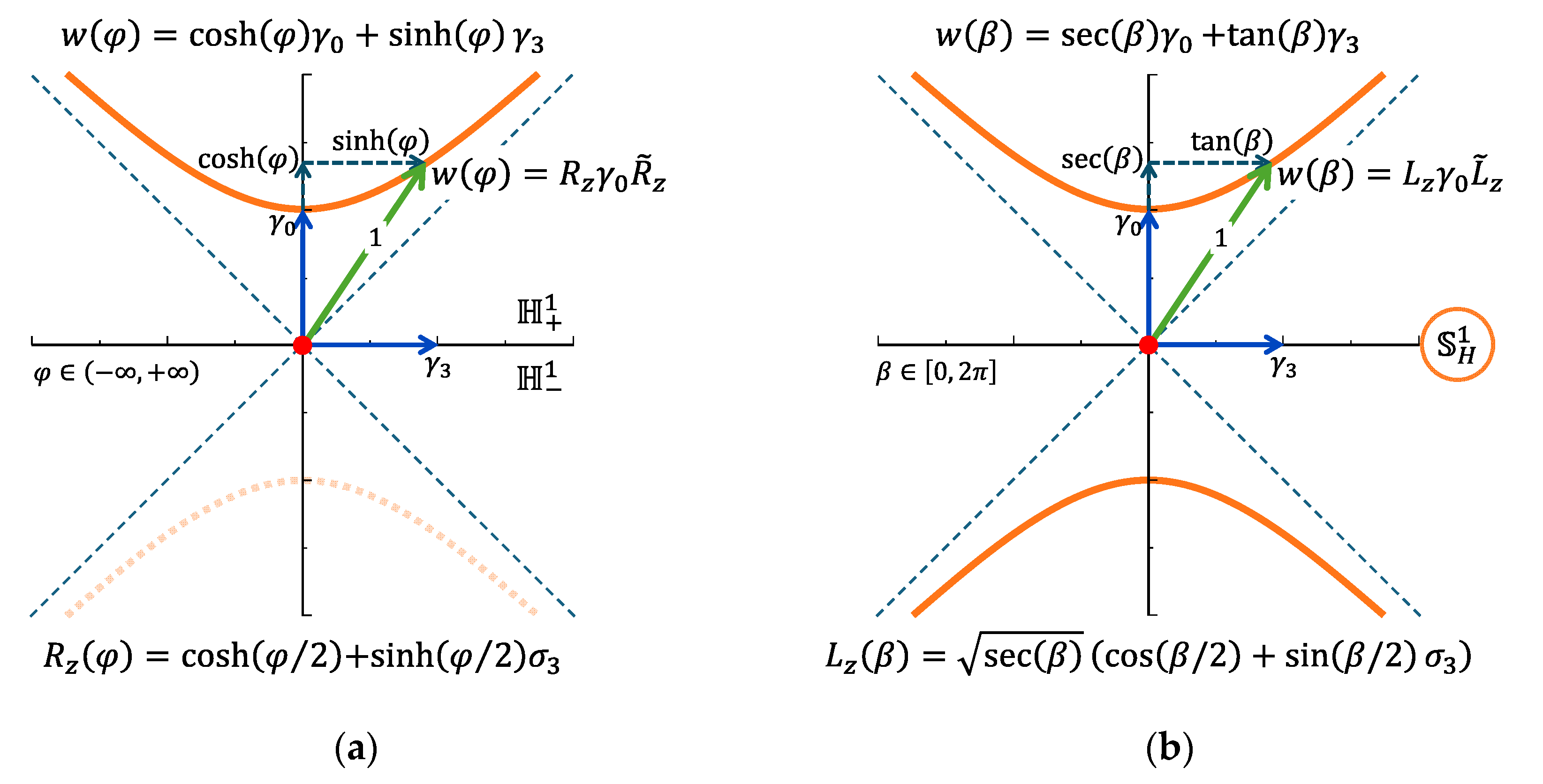
Figure 2.
(a) The spatial two-sphere spanned by vectors , is preserved by the
spatial spinor . (b) The hyperbolic three-sphere , spanned by vectors , is preserved by the spacetime rotor . The spatial vectors are all orthogonal to the temporal axis .
Figure 2.
(a) The spatial two-sphere spanned by vectors , is preserved by the
spatial spinor . (b) The hyperbolic three-sphere , spanned by vectors , is preserved by the spacetime rotor . The spatial vectors are all orthogonal to the temporal axis .
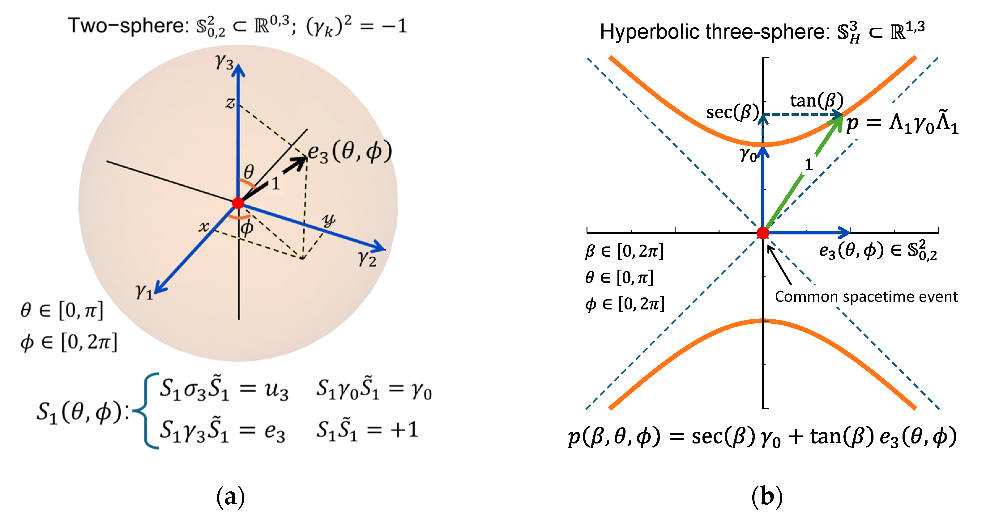
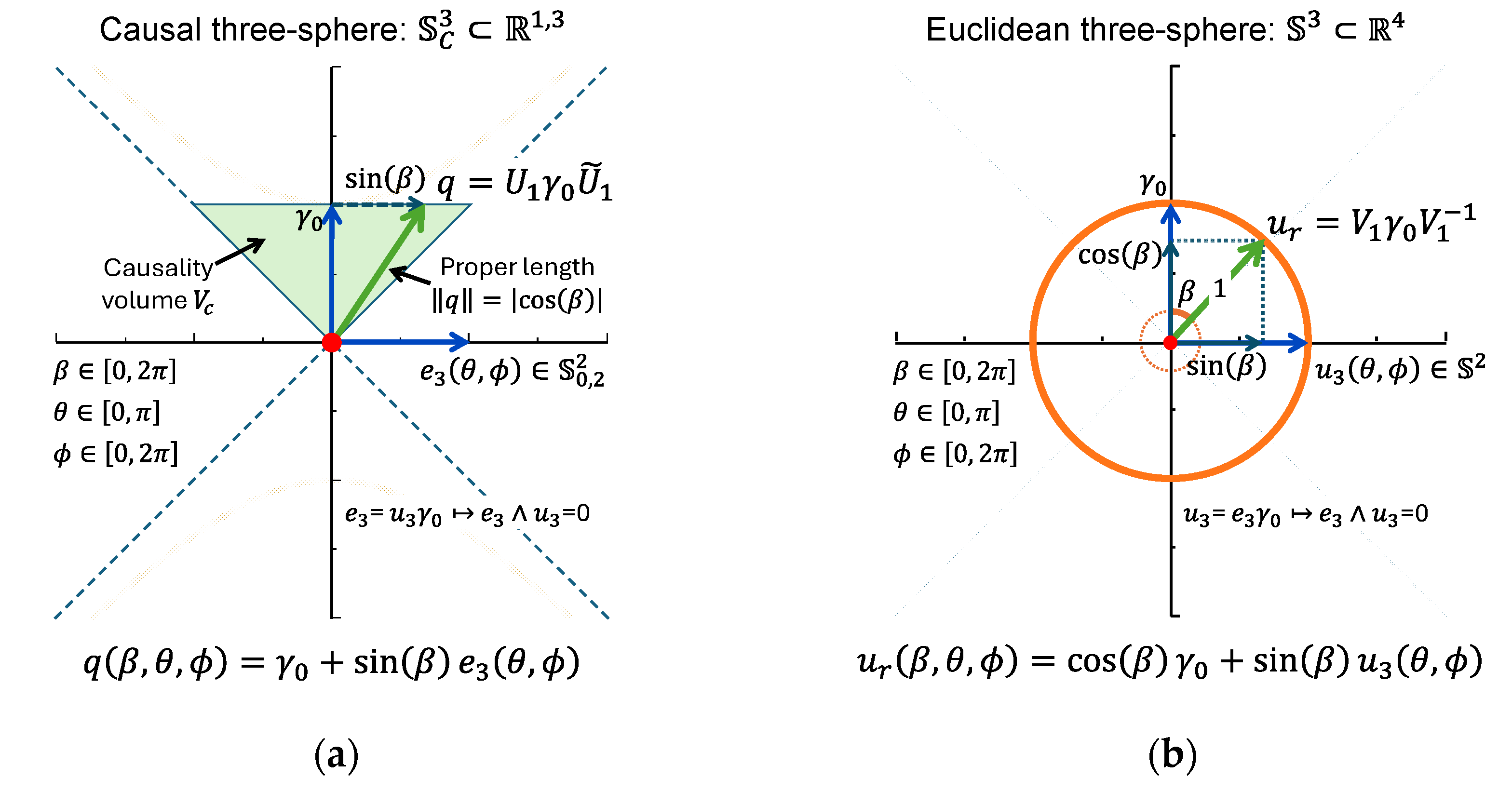
Figure 3.
(a) The causal three-sphere spanned by vectors , is preserved by the spacetime spinor . (b) The Euclidean three-sphere , spanned by vectors , is preserved by the Euclidean spinor . In this structure, each of the aligned vectors and is orthogonal to temporal
axis in its respective domain, thereby fixing a common
temporal bivector plane..
Disclaimer/Publisher’s Note: The statements, opinions and data contained in all publications are solely those of the individual author(s) and contributor(s) and not of MDPI and/or the editor(s). MDPI and/or the editor(s) disclaim responsibility for any injury to people or property resulting from any ideas, methods, instructions or products referred to in the content. |
© 2025 by the authors. Licensee MDPI, Basel, Switzerland. This article is an open access article distributed under the terms and conditions of the Creative Commons Attribution (CC BY) license (http://creativecommons.org/licenses/by/4.0/).
Copyright: This open access article is published under a Creative Commons CC BY 4.0 license, which permit the free download, distribution, and reuse, provided that the author and preprint are cited in any reuse.


