Submitted:
19 December 2025
Posted:
23 December 2025
You are already at the latest version
Abstract
Driven by global initiatives to mitigate climate change, the offshore wind power industry is experiencing rapid growth. Personnel transfer between service operation vessels (SOVs) and offshore wind turbines under complex sea conditions remains a critical factor governing the safety and efficiency of operation and maintenance (O&M) activities. This study establishes a fully coupled dynamic response and control simulation framework for an SOV equipped with an active motion-compensated gangway. A numerical model of the SOV is first developed using potential flow theory and frequency-domain multi-body hydrodynamics to predict realistic vessel motions, which serve as excitation inputs to a co-simulation environment (MATLAB/Simulink coupled with MSC Adams) representing the Stewart platform-based gangway. To address system nonlinearity and coupling, a composite control strategy integrating velocity and dynamic feedforward with three-loop PID feedback is proposed. Simulation results demonstrate that the composite strategy achieves an average disturbance isolation degree of 21.81 dB, significantly outperforming traditional PID control. Validation is conducted using a ship motion simulation platform and a combined wind-wave basin with a 1:10 scaled prototype. Experimental results confirm high compensation accuracy, with heave variation maintained within 1.6 cm and a relative error between simulation and experiment of approximately 18.2%.
Keywords:
active motion compensated gangway
; composite control strategy
; hydrodynamics
; service operational vessel
1. Introduction
The global energy landscape is undergoing a profound transformation, driven by the urgent need to decarbonize power generation and ensure energy sustainability. Offshore wind energy, characterized by its high energy density and low turbulence, has emerged as a cornerstone of this transition. According to the Global Wind Energy Council [1], the global offshore wind capacity is projected to surge significantly over the coming decade, with a marked trend towards installations in deeper waters (depths > 50m) where wind resources are more abundant and consistent [2,3]. As wind farms scale up and move further from shore, effective operation and maintenance (O&M) is pivotal for minimizing the Levelized Cost of Energy (LCOE), as it typically accounts for 25-30% of the total lifecycle cost of an offshore wind farm [4]. While traditional Crew Transfer Vessels (CTVs) have served the industry well in near-shore waters, they are generally limited to significant wave heights () of approximately 1.5 meters due to the safety risks associated with the friction-based "push-on" transfer method [5]. To ensure accessibility in more severe seas (m), the industry is increasingly relying on Service Operation Vessels (SOVs) equipped with active motion compensated gangways [6].
The fundamental operational objective of motion compensated gangway is to mechanically isolate the transfer bridge from the vessel’s 6-Degree-of-Freedom (6-DOF) wave-induced motions [7], thereby establishing a geostationary connection with the wind turbine platform, as shown in Figure 1. The mechanical design typically employs a Stewart-Gough parallel topology [8], chosen for its high stiffness-to-weight ratio and precise positioning capabilities. The hexapod-based motion compensated platform, commercially pioneered by companies like Ampelmann (shown in Figure 2) and Uptime is now central to offshore wind access [9]. Given the safety-critical nature of offshore "Walk-to-Work" (W2W) systems, the dynamic analysis and control of gangway have attracted extensive research interest.
In terms of control strategies for gangway, proportional-integral-derivative (PID) control remains the industrial standard due to its simplicity and robustness, yet its performance deteriorates markedly under stochastic wave disturbances and nonlinear actuator dynamics (e.g., cylinder hysteresis and friction), often amplifying tracking errors by 20–50 % in non-Gaussian sea states [10]. To address these limitations, model predictive control (MPC) has been widely adopted for its explicit constraint-handling capability (joint limits, power bounds), achieving up to 30 % reduction in peak error through receding-horizon optimisation [11,12]. More recently, active disturbance rejection control (ADRC) employing extended state observers has demonstrated superior disturbance attenuation, limiting residual 6-DOF motion to less to 5 % RMS in coupled vessel–gangway–turbine simulations under ranging from 2.5 m to 3.0 m [13]. Concurrently, neural-network-enhanced approaches futher improve the control precision under highly uncertain motion. An adaptive control method based on a backpropagation (BP)-PID control algorithm can reduce the position deviation by about 6.56 times compared with PID [14]. Similarly, the compensation errors could be decreased by 70% (roll or pitch) and 40% (heave) by the adaptive control strategy consisting of Beetle Antennae Search (BAS) algorithm and Radial Basis Function Neural Network (RBFNN) [15]. In addition to control algorithms, SOV can also improve operational efficiency through equipment selection. Small Waterplane Area Twin Hull (SWATH) is considered a superior option with higher operability compared to traditional monohull design [16]. Moreover, the integration of dynamic positioning systems with advanced trajectory prediction algorithms [17] further enhances the offshore operational efficiency of SOVs.
Despite these theoretical advancements, a critical limitation persists in the modeling fidelity of the "SOV-Gangway-Turbine" coupled system. The majority of control-oriented studies simplify the motion of SOV by simulating it with simple harmonic motion and random motion. This decoupled approach neglects the significant hydrodynamic interaction—specifically radiation and diffraction effects—that occurs when a large-displacement vessel operates in proximity to an offshore wind turbine [18,19]. Nearby offshore wind turbine structures can generate a clear shielding effect [20] that reduces wave loads on the service operation vessel. Conversely, under specific relative positions and wave headings, they may induce local wave amplification or altered diffraction [21,22], significantly deviating the vessel’s motion from simplified assumptions. It is essential to fully couple the gangway simulation with the dynamic system of the SOV and offshore wind turbine with experimental verification. Neglecting these multi-body interactions can lead to inaccurate predictions of the gangway’s required compensation, potentially compromising operational safety [23]. Furthermore, there is a distinct geographical gap in existing research: while extensive studies focus on North Sea conditions, there is a lack of systematic research tailored to the specific operational environment of the South China Sea [24], which is emerging as a major hub for offshore wind development.
To address these gaps, this paper presents a systematic study on the design, high-fidelity simulation, and validation of a vessel-borne active motion compensated gangway. The integrated workflow of this study—from wave-induced vessel dynamics and gangway control design to experimental validation—is conceptually outlined in Figure 3. The primary contributions are:
- (1)
- Precise Hydrodynamic Calculations: Unlike studies relying on rough wave models, we establish a numerical framework that explicitly calculates the time-domain hydrodynamic response of SOV. This captures the shielding and radiation effects, providing a high-fidelity prediction of the vessel’s relative motion.
- (2)
- Composite Control Strategy: We propose an optimized composite control strategy that augments a robust feedback architecture with feedforward compensation. This approach is specifically tuned to handle the complex relative motions predicted by our coupled hydrodynamic model.
- (3)
- Scaled Experimental Validation: We designed and constructed a scaled prototype of the gangway system and validated its performance using a dual-Stewart platform setup. A large 6-DOF Stewart platform acts as the motion simulator to replicate the precise vessel motions calculated from our hydrodynamic model, while the prototype gangway (a smaller Stewart platform) performs active compensation, bridging the gap between theoretical simulation and physical reality.
This paper is organized as follows: Section 2 details the theoretical background, including hydrodynamics of SOV and the kinematic and dynamic modeling of the gangway. Section 3 describes the co-simulation framework and comparative analysis of control strategies. The simulation process and results are displayed in Section 4. Section 5 presents the design of the scaled prototype and discusses the experimental results, followed by the conclusion in Section 6.
2. Theoretical Background
This section provides a detailed introduction to the theoretical basis of the ship-borne active motion compensated gangway. It mainly includes hydrodynamics of SOV, kinematic and dynamic models of gangways, and control strategies.
2.1. Hydrodynamics of the Service Operation Vessel
Hydrodynamic analysis of the SOV is essential for accurately predicting its 6-DOF motions when operating adjacent to fixed-bottom offshore wind turbine platforms. These motion responses provide the primary external disturbances for evaluating the performance and safety of the vessel-borne active motion-compensated gangway during walk-to-work operations.
The theoretical framework is based on linear potential flow theory, assuming an inviscid, incompressible, and irrotational fluid. The flow field is described by a velocity potential . The SOV is modelled as a rigid body with six degrees of freedom: surge, sway, heave, roll, pitch, and yaw. Two right-handed coordinate systems are employed: an Earth-fixed inertial system - and a body-fixed system - with its origin at the vessel’s centre of gravity (COG). All hydrodynamic computations and equations of motion are formulated in the body-fixed frame.
The spatial velocity potential is decomposed as
where are radiation potentials due to unit-amplitude motion in the j-th mode, is the unit-amplitude incident wave potential in deep water, is the diffraction potential, is the incident wave amplitude, and are complex motion amplitudes. Each potential satisfies the Laplace equation in the fluid domain, the linearized free-surface condition, the hull impermeability condition, and the far-field radiation condition.
The frequency-domain boundary value problem is solved using the boundary element method (BEM) with a free-surface Green function [25]. From the solved potentials, the frequency-dependent added mass and radiation damping are obtained from the radiation potentials:
The first-order wave exciting force is computed from the incident and diffracted fields:
where is seawater density and H is the mean wetted hull surface.
The time-domain motion is described by Cummins’ equation [26], which accounts for fluid memory effects via a convolution term:
where is the vessel’s mass matrix, is the infinite-frequency added mass, is the retardation function matrix, and are frequency-independent linear and quadratic viscous damping matrices calibrated from decay tests, is the hydrostatic restoring matrix, and is the external force vector.
The retardation function is obtained from the frequency-domain damping via the cosine transform [27]:
In practice, artificial decay is applied to outside the computed frequency range, and is truncated when its magnitude becomes negligible. The infinite-frequency added mass is evaluated using
where is an arbitrary frequency within the solved range; results are averaged over several for robustness.
Irregular wave elevation is generated from the target JONSWAP spectrum as
with
where X and Y are the low-frequency horizontal position in the global system, is the mean wave direction, satisfies the deep-water dispersion relation [28], are random phases, and
The corresponding first-order wave force is
where and are the magnitude and phase of the force transfer function, interpolated at each time step to reflect heading changes.
Equation (4) is integrated using a fourth-order Runge–Kutta scheme with a time step of typically 0.02–0.05 s. The convolution is evaluated numerically using the precomputed . Multiple 3-hour realisations with independent random phase sets are performed to ensure statistical convergence. The resulting high-fidelity 6-DOF motion time histories at the COG [29] are transformed to the global frame and used as disturbance inputs to the gangway control co-simulation. The hydrodynamic computations described above were performed using HydroStar [30], a frequency-domain 3D diffraction/radiation analysis software. HydroStar computes the key hydrodynamic coefficients—including added mass, radiation damping, and wave excitation forces—which were subsequently exported and integrated into our custom time-domain solver, Kraken[31,32].
2.2. Kinematic and Dynamic Models of Gangways
The kinematic analysis of the Stewart platform is essential for motion compensation control. The position, velocity, and acceleration relationships between the moving platform and the actuator legs are derived using the closed-loop vector method.The structure of the Stewart platform is shown in the Figure 4.
The position vector of the i-th leg can be expressed as:
where and denote the position vectors of the upper and lower hinge points in the global inertial coordinate system, respectively, and is the translation vector of the moving platform.
The length of the i-th leg is given by:
The unit vector along the leg is:
The velocity of the leg is derived as:
where and are the velocities of the upper and lower hinge points, respectively.
The acceleration of the leg is obtained as:
where is the angular velocity of the leg.
The Jacobian matrices for the upper and lower platforms are defined as:
The dynamic model of the Stewart platform is established using Kane’s method to account for the non-inertial base motion. The generalized coordinates of the moving platform are defined as:
The generalized velocities are:
The partial velocities and partial angular velocities are derived for the platform, legs, and payload. The generalized active and inertial forces are formulated as:
The final dynamic equation is expressed as:
where and are mass matrices of the upper and base platforms, and are Coriolis and centrifugal force vectors, is the gravity vector, and is the driving force vector of the legs.
The electric cylinder, driven by a permanent magnet synchronous motor (PMSM), is modeled as:
where is the q-axis current, is the motor angular velocity, is the stator resistance, is the q-axis inductance, is the back EMF coefficient, is the torque coefficient, is the rotor inertia, is the damping coefficient, is the q-axis voltage, and is the load torque.
The transfer function from voltage to angular velocity is:
The linear displacement of the electric cylinder is related to the motor rotation by:
where P is the screw lead, n is the transmission efficiency, and is the motor angle.
This completes the theoretical foundation for the kinematic and dynamic modeling of the motion-compensated gangway based on the Stewart platform.
2.3. Control Strategies
2.3.1. PID Control
In motion compensation systems based on the Stewart parallel mechanism, the design of control strategies is crucial to achieve high-precision trajectory tracking and effective disturbance rejection. The system exhibits strong nonlinearity, coupling, and time-varying characteristics due to its multi-input multi-output (MIMO) structure and the complex marine environment in which it operates. This section introduces the fundamental control methodologies employed, namely PID control and feedforward control, which form the basis of the proposed composite control strategy.
PID control is one of the most widely used control strategies in industrial applications due to its simplicity, robustness, and ease of implementation. The continuous-time form of a PID controller is expressed as:
where is the control output, is the error between the desired and actual output, and , , and are the proportional, integral, and derivative gains, respectively.
In the context of the Stewart platform, a three-loop control structure is typically adopted for each electric cylinder, comprising current loop, velocity loop and position loop. The current loop is the innermost loop regulated the motor torque using a PI controller to ensure fast response and disturbance rejection. The velocity loop, which is the middle control loop, regulates the motor speed using a PI controller to improve dynamic performance. The position loop is the outer loop, which achieves accurate position tracking, often using a P or PID controller.
The PID parameters are usually tuned sequentially from the inner to the outer loop. However, due to the nonlinear and coupled nature of the Stewart platform, conventional tuning methods may not suffice. Thus, intelligent optimization techniques such as the Genetic Algorithm (GA) are employed to auto-tune the PID parameters by minimizing a cost function that considers tracking error, overshoot, and settling time.
2.3.2. Feedforward Control
To enhance the tracking performance and robustness of the PID controller, feedforward control is introduced. Unlike the feedback control, which reacts to errors, feedforward control proactively compensates for known disturbances or system dynamics.
Velocity feedforward is used to improve the tracking of high-frequency reference signals by utilizing the high bandwidth of the velocity loop. The feedforward term is derived from the derivative of the desired position signal:
where is the desired position of the electric cylinder, and is the velocity feedforward gain. When properly designed, this term reduces phase lag and improves the system’s ability to track dynamic trajectories.
Dynamics feedforward compensates for the nonlinear and coupling effects within the Stewart platform. Based on the inverse dynamics model, the required control force for each actuator is computed and fed forward to the current loop:
where F is the axial force computed from the dynamics model, and is the motor torque constant. This approach mitigates the effects of inertial and coupling forces, thereby improving both dynamic response and disturbance rejection.
2.3.3. Composite Control Strategy
By integrating both PID feedback and feedforward control, a composite control strategy is formed. This hybrid approach leverages the error-correction capability of PID and the predictive compensation of feedforward control, resulting in enhanced performance in terms of tracking accuracy, response speed, and stability—even under complex multi-degree-of-freedom disturbances.
The overall control law for each actuator can be summarized as:
where is the output of the PID controller, is the velocity feedforward term, and is the dynamics feedforward term.
This composite strategy has been validated through both simulation and experimentation, demonstrating significant improvements in motion compensation performance for the Stewart-based gangway system.
3. Establishment of Numerical Models and Simulation Models
3.1. Numerical Model Implementation
The theoretical models derived in previous sections were implemented numerically to enable digital simulation and analysis. This process involved discretizing the continuous-time equations and developing efficient computational algorithms.
3.1.1. Kinematic Numerical Solution
The inverse kinematics solution was implemented using vector operations. For each sampling time step, the leg lengths were computed as:
where k denotes the discrete time index, and are the rotation matrices of the moving and base platforms at time step k, and and are their translation vectors.
The Jacobian matrices were computed numerically at each time step to handle the system’s nonlinearity:
3.1.2. Dynamic Numerical Integration
The Kane’s dynamic equations were solved using numerical integration methods. The fourth-order Runge-Kutta method was employed for its balance between accuracy and computational efficiency:
where to are the intermediate derivatives computed at different points within the time step .
3.2. Simulation Framework Construction
A co-simulation framework was established using MATLAB/Simulink and Adams to leverage the strengths of both platforms for control system design and multi-body dynamics analysis.
3.2.1. Multi-body Dynamics Model in Adams
The mechanical system was modeled in Adams with precise geometric and mass properties, as detailed in Table 1.
The electric cylinders are connected to the upper platform via spherical joints (3 DOFs) and to the lower platform via universal joints (2 DOFs), while their actuation is provided by internal prismatic joints (1 DOF).
3.2.2. Control System Model in Simulink
The control system was implemented in Simulink, as shown in Figure 5. The main components included Disturbance Generator, Inverse Kinematics Module, Controller Module, Adams Interface. Disturbance Generator provides 6-DOF motion of the SOV computed in Section 2.1. Inverse Kinematics Module computed desired leg lengths from platform poses. Controller Module implemented the composite feedforward-feedback control strategy. Adams Interface handled data exchange with the Adams mechanical model.
4. Simulation and Result
4.1. Simulation Parameters and Conditions
The long-term distribution probability of wave conditions in the operating sea area will directly affect the window period of operation and maintenance, and the wave scatter diagram is generally used to describe such distribution probability. The sea-state calculations in this paper are conducted using wave data from the South China Sea (off Guangdong, China), given the region’s significance as a major hub for China’s expanding offshore wind power sector. Therefore, the scatter diagram in this study (Figure 6) are based on historical wave data from [33], with the peak period converted according to the method of [34].
The irregular wave field was generated based on the JONSWAP spectrum, with the governing parameters given as follow: the sea state is characterized by a significant wave height () of and a peak period () of . A standard peak enhancement factor () of and a spectral shape parameter () of 0 were applied. To ensure sufficient resolution in the frequency domain, the spectrum was discretized over a range of with a frequency increment of . The generated JONSWAP wave spectrum is shown in the Figure 7.
Ultimately, the total surface elevation time series is constructed through the linear superposition of these individual harmonic components, often calculated using an Inverse Fast Fourier Transform, resulting in a realistic simulation of an irregular wave field that statistically matches the target JONSWAP spectrum, the wave height shown in the Figure 8.
Figure 9 shows the monohull SOV model studied in this paper, and Table 2 lists its key specifications. Figure 10 presents the corresponding amplitude-frequency response operator (RAO), calculated using the method described in Section 2.1. Finally, Figure 11 shows 600-second excerpts of the resulting 6-DOF motion time histories. These time histories were computed by applying the wave excitation forces to the vessel’s RAOs. The full simulation represented a three-hour operational scenario, but for clarity, only a representative segment is displayed here.
In this study, the motion of the lower platform of the motion compensated gangway installed on the vessel can be obtained through coordinate transformation. Since the base of the Stewart platform is rigidly connected to the deck, its attitude remains consistent with the vessel, and coordinate transformation only needs to be performed for the translational directions. The base platform of the Stewart platform should be installed on the Y-direction axis, at the intersection with the vertical line passing through the center of mass, to reduce the impact of vessel motion. Its specific coordinates relative to the vessel coordinate system are (-26, 0, -5.8). The displacement of the Stewart platform’s base obtained through coordinate transformation is shown in the Figure 12.
Assuming the ideal state where the upper platform is fully compensated (i.e., the upper platform remains stationary relative to the inertial coordinate system), the length variations of the six legs can be calculated after obtaining the 6-DOF motion time histories of the Stewart platform’s base relative to the inertial coordinate system, as shown in the Figure 13.
4.2. Simulation Results and Analysis
To further compare the control motion compensation effect under the traditional PID control with the composite control strategy, input the base platform’s pose and leg length changes into the motion compensated gangway system built by Simulink-Adams, and obtain the six-degree-of-freedom motion time history and acceleration of the Stewart upper platform, the result for using PID control as shown in the Figure 14 and Figure 15.
Next, velocity and dynamic feedforward are introduced, and the simulation results are obtained as shown in the Figure 16 and Figure 17.
The compensation performance was quantified using the isolation degree metric.Define the compensation isolation degree as the evaluation index for the compensation effect of the motion compensated gangway system in each degree of freedom, which is expressed by Equation (31).
In the formula, is the value of the motion compensated gangway in a certain degree of freedom, and is the value of the pose simulation platform in the corresponding degree of freedom. The larger is, the better the compensation effect of the motion compensated gangway on disturbances; when it is infinite, it indicates complete compensation for disturbances. Conversely, the closer it is to 0, the worse the compensation effect; when it is 0, it means the platform has no compensation effect on disturbances at all.
Table 3 summarizes the isolation degrees achieved for each degree of freedom under different control strategies.
The composite control strategy demonstrated superior performance, achieving an average isolation degree of 21.81 dB, which corresponds to approximately 91% disturbance rejection.
5. Scaled Gangway Prototype Experiment
5.1. Experimental Platform Design and Setup
To validate the simulation results and control strategies, a 1:10 Scaled experimental platform was designed and constructed, maintaining geometric and dynamic similarity with the full-scale system.
The experimental setup of the Stewart platform mainly includes a dual-layer Stewart-configuration mechanical structure, an AC servo system, an inertial measurement unit (IMU), a motion control card, and a PC upper computer.
The mechanical system of this experimental setup is mainly composed of two parts: a motion simulation subsystem and a motion compensated subsystem. The lower Stewart platform serves as the motion simulation system, which can provide six-degree-of-freedom motion simulating an offshore operation and maintenance vessel. The upper Stewart platform acts as the motion compensated system, whose lower plane is welded and fixed to the upper plane of the lower Stewart platform. It is actuated by a complete set of control systems and electric cylinders to compensate for the motion caused by the lower Stewart platform and maintain the stability of the upper plane. The physical diagram of the dual-layer Stewart-configuration mechanical structure is shown in Figure 18.
The key technical parameters of both Stewart platforms are detailed in Table 4.
The motion compensated control system uses a motion control card as the main controller. An inertial motion sensor, serving as the pose measurement and feedback component, is installed at the center of the base platform of the Stewart platform to feed back the real-time pose information of the lower plane of the motion compensated system to the upper computer software. After undergoing steps such as signal preprocessing, signal prediction, and forward/inverse kinematic solutions, the upper computer calculates the rod length error of each electric cylinder and sends control commands to the motion control card. The motion control card drives the motor operation by controlling the driver; the motor drives the expansion and contraction of the electric cylinder through a mechanical transmission mechanism to complete the control of a single joint branch. Ultimately, it achieves the control of the upper plane of the motion compensated system, keeping it in a relatively stable state at all times. The entire experimental setup is shown in the Figure 19.
5.2. Control System Implementation
During the operation of the motion compensated system, it is necessary to perform kinematic and dynamic model calculations based on the disturbance pose signals detected by the inertial motion sensor, and then control the electric cylinders to compensate for ship disturbances.
Among the disturbance poses in six degrees of freedom, the angles of roll, pitch, and yaw can be obtained by a high-precision attitude and heading reference system. However, the displacement data of surge, sway, and heave cannot be directly measured and need to be obtained through double integration of acceleration information in the corresponding directions. The acceleration information measured by the sensor contains noise and interference from low-frequency Schuler period oscillation signals, and especially interference from gravitational acceleration in the heave direction. Therefore, the original acceleration information needs to be further processed to obtain a more accurate calculated value of heave motion.
In the pose calculation module, to achieve accurate estimation of disturbance motions such as platform heave, this paper adopts the Cubature Kalman Filter (CKF) algorithm for state estimation of the received original sensor data. Compared with the traditional Extended Kalman Filter (EKF) method, the Cubature Kalman Filter has higher accuracy and stability when dealing with nonlinear systems, making it more suitable for the calculation of complex motion states in the marine environment.
5.3. Experimental Protocol
To ensure the experimental results could be extrapolated to the full-scale system, similarity criteria were strictly followed. Based on Froude similarity law, the time scaling factor was determined as:
where s is the prototype wave period and is the geometric scale ratio.
During the compensation experiment, one pose measurement unit is placed on the upper plane of the pose simulator to measure the disturbed pose, and another pose measurement unit is placed on the stable compensation plane to verify the effect of stable compensation. A laser range finder is fixed at the same position as the pose measurement unit to measure the displacement variation in the heave direction, with a measurement accuracy of 2mm. The pose simulation platform is used to simulate disturbances in each degree of freedom, and the attitude angle changes of the motion compensated platform are obtained through the pose measurement units.
5.4. Experimental Results and Analysis
To ensure that the experimental results can effectively reflect the actual force and response laws of the prototype structure, real sea conditions must be considered in the scaled model experiment. For better verifying the reliability of motion compensation and the effectiveness of the scaled test, we added two other common sea state conditions as inputs, which are and . The wave direction set to 90° beam sea, it may cause relatively strong roll, which poses great challenges to the system stability. The wave conditions are summarized in Table 5.
A 20-second 6-DOF motion time history is input into the motion control software of the pose simulation platform, and the pose measured by the motion compensated platform is shown in Figure 20.
The analysis results show that the variation of the platform’s attitude angles is kept within , and the isolation degrees of roll angle, pitch angle, and yaw angle reach 16.48 dB. Measurements from the laser range finder indicate that the variation in the heave direction is between 1.399 m and 1.414 m, i.e., the heave variation is maintained within a small range of 1.4 cm with an isolation degree of 15.14 dB.
The simulation results corresponding to the time points in the previous text are scaled by a scale ratio of 1:10, and the difference is calculated between these scaled results and the model test results after low-pass filtering.
The error results between model test and simulation are shown in Figure 21. Tests show that the angle error is less than 0.03°, and the displacement error is less than 0.01m.
The pose measured by the motion compensated platform and the error between model test and simulation are shown in Figure 22, Figure 23, Figure 24, and Figure 25.
The analysis results show: When , , the variation of the platform’s attitude angles is kept within 0.5°, and the isolation degrees of angles reach 15.25 dB. the heave variation is maintained within a small range of 1.6 cm with an isolation degree of 13.02 dB. When , , the variation of the platform’s attitude angles is kept within 0.8°, and the isolation degrees of angles reach 13.17 dB. the heave variation is maintained within a small range of 1.4 cm with an isolation degree of 12.14 dB. The calculated average error rate is 18.2%, which can meet the requirements for experimental verification of the simulation results.
6. Results and Discussion
6.1. Performance Analysis of Control Strategies
The simulation results presented in Section 4 demonstrate the efficacy of the proposed control strategies for the vessel-borne active motion compensated gangway. As illustrated in the comparative analysis between the traditional PID control and the proposed composite control strategy, the latter significantly enhances motion compensation performance.
Specifically, the composite control strategy achieved an average isolation degree of 21.81 dB across all six DOFs, compared to 18.15 dB for the standard PID controller (see Table 3). This represents an improvement of approximately 3.66 dB. Notably, the heave and pitch motions—critical for personnel safety during transfer—saw isolation degrees increase to 21.58 dB and 23.12 dB, respectively. This superior performance is attributed to the feedforward loop’s ability to proactively compensate for wave-induced disturbances based on the inverse dynamics model, thereby reducing the phase lag and tracking errors inherent in pure feedback systems. The results indicate that the system can effectively reject approximately 91% of disturbances, ensuring a stable gangway tip position even under irregular wave conditions defined by the JONSWAP spectrum.
6.2. Experimental Validation and Model Fidelity
The experimental trials conducted on the 1:10 scaled prototype in the wave-wind combined test basin provided physical validation for the numerical models. Under simulated sea states corresponding to the specific wave scatter diagram of the Guangdong offshore wind farm, the prototype maintained high stability. The attitude angle variations were constrained within , and the residual heave motion was maintained within a small range of 1.6 cm. The experimental isolation degrees reached 16.48 dB for rotational motions and 15.14 dB for heave, confirming the mechanical feasibility of the design.
A critical aspect of this study was validating the fully coupled SOV-Gangway-Turbine dynamic system. The comparison between the scaled simulation results and the model test data yielded an average error rate of 18.2%. While this discrepancy exists, it is within the acceptable range for complex hydrodynamic and multi-body mechanical coupling problems. The error can be attributed to unmodeled non-linear factors such as mechanical friction in the electric cylinders, sensor noise (drift in accelerometer integration), and complex viscous fluid effects that potential flow theory estimates with lower precision. Nevertheless, the correlation confirms that the developed simulation framework is sufficiently accurate for predicting system behavior and optimizing control parameters for full-scale applications.
7. Conclusions
This paper presented a comprehensive study on the simulation and experimental validation of a vessel-borne active motion compensated gangway designed for offshore wind operation and maintenance. By establishing a fully coupled hydrodynamic and mechanical model and proposing a composite control strategy, the following conclusions are drawn:
- Integrated Simulation Framework: A numerical model integrating frequency-domain multi-body hydrodynamics with time-domain mechanical dynamics was successfully developed. This framework effectively captures the complex interactions between the SOV, the motion-compensated gangway, and the fixed offshore wind turbine.
- Enhanced Control Performance: The proposed active motion compensated strategy, which combines feedforward control (velocity and dynamics) with a three-loop PID feedback structure, demonstrated superior performance over traditional methods. Simulation results confirmed an average disturbance isolation degree of 21.81 dB, effectively neutralizing over 90% of vessel motions.
- Experimental Validation: A 1:10 scaled prototype was constructed and tested. The experimental results validated the simulation, with the heave variation maintained within 1.6 cm and a simulation-to-experiment error margin of 18.2%. This verifies the reliability of the theoretical model and the control system design.
Future work will focus on minimizing the simulation-experiment discrepancy by refining friction models and incorporating advanced sensor fusion algorithms (e.g., Extended Kalman Filters) to further reduce noise in real-time heave estimation. Additionally, full-scale sea trials are planned to evaluate the system’s robustness under extreme weather conditions.
Author Contributions
Conceptualization, H.M., T.Z. and B.L.; methodology, H.M., T.Z. and B.L.; software, H.M.; validation, H.M. and T.Z.; formal analysis, H.M., T.Z., B.L. and K.L.; resources, B.L. and K.L.; writing—original draft, H.M. and T.Z.; writing—review and editing, H.M., T.Z., B.L. and K.L. ; visualization, H.M., T.Z.; supervision, B.L. and K.L.; funding acquisition, B.L. All authors have read and agreed to the published version of the manuscript.
Funding
This research was funded by the General Program of National Natural Science Foundation of China (52371280), the grant of international cooperation of science and technology, department of science and technology of Guangdong province (2023A0505050086), Guangdong joint research fund of offshore wind power (2023A1515240025).
Data Availability Statement
The original contributions presented in this study are included in the article. Further inquiries can be directed to the corresponding authors.
Conflicts of Interest
The authors declare no conflicts of interest.
References
- Global Wind Energy Council. Global Offshore Wind Report 2024. Technical report, Global Wind Energy Council, 2024. Accessed March 12, 2025.
- International Renewable Energy Agency. Future of Wind: Deployment, Investment, Technology, Grid Integration and Socio-economic Aspects. Technical report, International Renewable Energy Agency, Abu Dhabi, 2019.
- Díaz, H.; Guedes Soares, C. Review of the current status, technology and future trends of offshore wind farms. Ocean Engineering 2020, 209, 107381. [Google Scholar] [CrossRef]
- Ren, Z.; Verma, A.S.; Li, Y.; Teuwen, J.J.; Jiang, Z. Offshore wind turbine operations and maintenance: A state-of-the-art review. Renewable and Sustainable Energy Reviews 2021, 144, 110886. [Google Scholar] [CrossRef]
- O’Connor, M.; Lewis, T.; Dalton, G. Weather window analysis of Irish west coast wave data with relevance to operations & maintenance of marine renewables. Renewable Energy 2013, 52, 57–66. [Google Scholar] [CrossRef]
- Hong, S.; McMorland, J.; Zhang, H.; Collu, M.; Halse, K.H. Floating offshore wind farm installation, challenges and opportunities: A comprehensive survey. Ocean Engineering 2024, 304, 117793. [Google Scholar] [CrossRef]
- Salzmann, C.; Ampelmann, D. Development of the access system for offshore wind turbines. Delft: Delft University of Technology 2010. [Google Scholar]
- Stewart, D. A Platform with Six Degrees of Freedom. Proceedings of the Institution of Mechanical Engineers 1965, 180, 371–386. [Google Scholar] [CrossRef]
- Pergod, L.; Dighe, V.; Yung, C. Offshore Wind Access Report 2023. Technical Report TNO-2023-R12488, TNO, Petten, The Netherlands, 2023. [Google Scholar]
- Yin, L.; Qiao, D.; Li, B.; Liang, H.; Yan, J.; Tang, G.; Ou, J. Modeling and controller design of an offshore wind service operation vessel with parallel active motion compensated gangway. Ocean Engineering 2022, 266, 112999. [Google Scholar] [CrossRef]
- Woodacre, J.; Bauer, R.; Irani, R. Hydraulic valve-based active-heave compensation using a model-predictive controller with non-linear valve compensations. Ocean Engineering 2018, 152, 47–56. [Google Scholar] [CrossRef]
- Chen, X.; Jiao, Y.; Yuan, X.; Meng, Z.; Zhang, L.; Liu, X. An online dual-loop AMPC strategy for wave compensation of an electro-hydraulic servo Stewart platform. Control Engineering Practice 2025, 165, 106540. [Google Scholar] [CrossRef]
- Chen, W.; Wang, S.; Li, J.; Lin, C.; Yang, Y.; Ren, A.; Li, W.; Zhao, X.; Zhang, W.; Guo, W.; et al. An ADRC-based triple-loop control strategy of ship-mounted Stewart platform for six-DOF wave compensation. Mechanism and Machine Theory 2023, 184, 105289. [Google Scholar] [CrossRef]
- Li, D.; Wang, S.; Song, X.; Zheng, Z.; Tao, W.; Che, J. A BP-Neural-Network-Based PID Control Algorithm of Shipborne Stewart Platform for Wave Compensation. Journal of Marine Science and Engineering 2024, 12. [Google Scholar] [CrossRef]
- Liu, J.; Chen, X. Adaptive Control Based on Neural Network and Beetle Antennae Search Algorithm for an Active Heave Compensation System. International Journal of Control, Automation and Systems 2022, 20, 515–525. [Google Scholar] [CrossRef]
- Zhou, T.; Li, B.; Liu, K.; Huang, W.; Wang, C.; Yang, L. Accessibility of floating wind turbines via walk-to-work: SWATH vs. monohull service vessels. Ocean Engineering 2025, 342, 123043. [Google Scholar] [CrossRef]
- Zhang, Y.; Han, Z.; Zhou, X.; Li, B.; Zhang, L.; Zhen, E.; Wang, S.; Zhao, Z.; Guo, Z. METO-S2S: A S2S based vessel trajectory prediction method with Multiple-semantic Encoder and Type-Oriented Decoder. Ocean Engineering 2023, 277, 114248. [Google Scholar] [CrossRef]
- Li, B.; Ou, J. Heave response analysis of Truss Spar in frequency domain. The ocean engineering (In Chinese). 2009, 27, 8–15. [Google Scholar]
- Li, B.; Ou, J.P.; Teng, B. Fully Coupled Effects of Hull, Mooring and Risers Model in Time Domain Based on An Innovative Deep Draft Multi-Spar. China Ocean Engineering 2010, 24, 219–234. [Google Scholar]
- Li, B. Effect of hydrodynamic coupling of floating offshore wind turbine and offshore support vessel. Applied Ocean Research 2021, 114, 102707. [Google Scholar] [CrossRef]
- Jian, W.; Cao, D.; Lo, E.Y.; Huang, Z.; Chen, X.; Cheng, Z.; Gu, H.; Li, B. Wave runup on a surging vertical cylinder in regular waves. Applied Ocean Research 2017, 63, 229–241. [Google Scholar] [CrossRef]
- Wang, X.; Qiao, D.; Jin, L.; Yan, J.; Wang, B.; Li, B.; Ou, J. Numerical investigation of wave run-up and load on heaving cylinder subjected to regular waves. Ocean Engineering 2023, 268, 113415. [Google Scholar] [CrossRef]
- Yang, L.; Li, B.; Dong, Y.; Hu, Z.; Zhang, K.; Li, S. Large-amplitude rotation of floating offshore wind turbines: A comprehensive review of causes, consequences, and solutions. Renewable and Sustainable Energy Reviews 2025, 211, 115295. [Google Scholar] [CrossRef]
- Hasager, C.B.; Astrup, P.; Zhu, R.; Chang, R.; Badger, M.; Hahmann, A.N. Quarter-Century Offshore Winds from SSM/I and WRF in the North Sea and South China Sea. Remote Sensing 2016, 8. [Google Scholar] [CrossRef]
- Li, B.; Liu, Z.; Liang, H.; Zheng, M.; Qiao, D. BEM modeling for the hydrodynamic analysis of the perforated fish farming vessel. Ocean Engineering 2023, 285, 115225. [Google Scholar] [CrossRef]
- Cummins, W.E. The Impulse Response Function and Ship Motions. Schifstechnik 1962, 9, 101–109. [Google Scholar]
- Ogilvie, T. Recent progress toward the understanding and prediction of ship motions. Proceedings of the 5th Symposium on Naval Hydrodynamics 1964. [Google Scholar]
- Newman, J.N. Marine Hydrodynamics; The MIT Press, 1977. [Google Scholar] [CrossRef]
- Li, B.; Liang, H.; Chen, X.; Araujo, R. Study of telescopic gangway motions in time domain during offshore operation. Ocean Engineering 2021, 230, 108692. [Google Scholar] [CrossRef]
- Bureau Veritas. HydroStar for Experts User Manual; Bureau Veritas, 92571 Neuilly-Sur-Seine, France, v8.10 ed., 2021.
- Li, B.; Wang, C. The absolute nodal coordinate formulation in the analysis of offshore floating operations Part I: Theory and modeling. Ocean Engineering 2023, 281, 114645. [Google Scholar] [CrossRef]
- Wang, C.; Liu, J.; Li, B.; Huang, W. The absolute nodal coordinate formulation in the analysis of offshore floating operations, Part II: Code validation and case study. Ocean Engineering 2023, 281, 114650. [Google Scholar] [CrossRef]
- Lin, Y.; Dong, S.; Wang, Z.; Guedes Soares, C. Wave energy assessment in the China adjacent seas on the basis of a 20-year SWAN simulation with unstructured grids. Renewable Energy 2019, 136, 275–295. [Google Scholar] [CrossRef]
- Li, B.; Qiao, D.; Zhao, W.; Hu, Z.; Li, S. Operability analysis of SWATH as a service vessel for offshore wind turbine in the southeastern coast of China. Ocean Engineering 2022, 251, 111017. [Google Scholar] [CrossRef]
Figure 1.
Offshore Walk-to-Work Scenario. (Courtesy of ESVAGT).
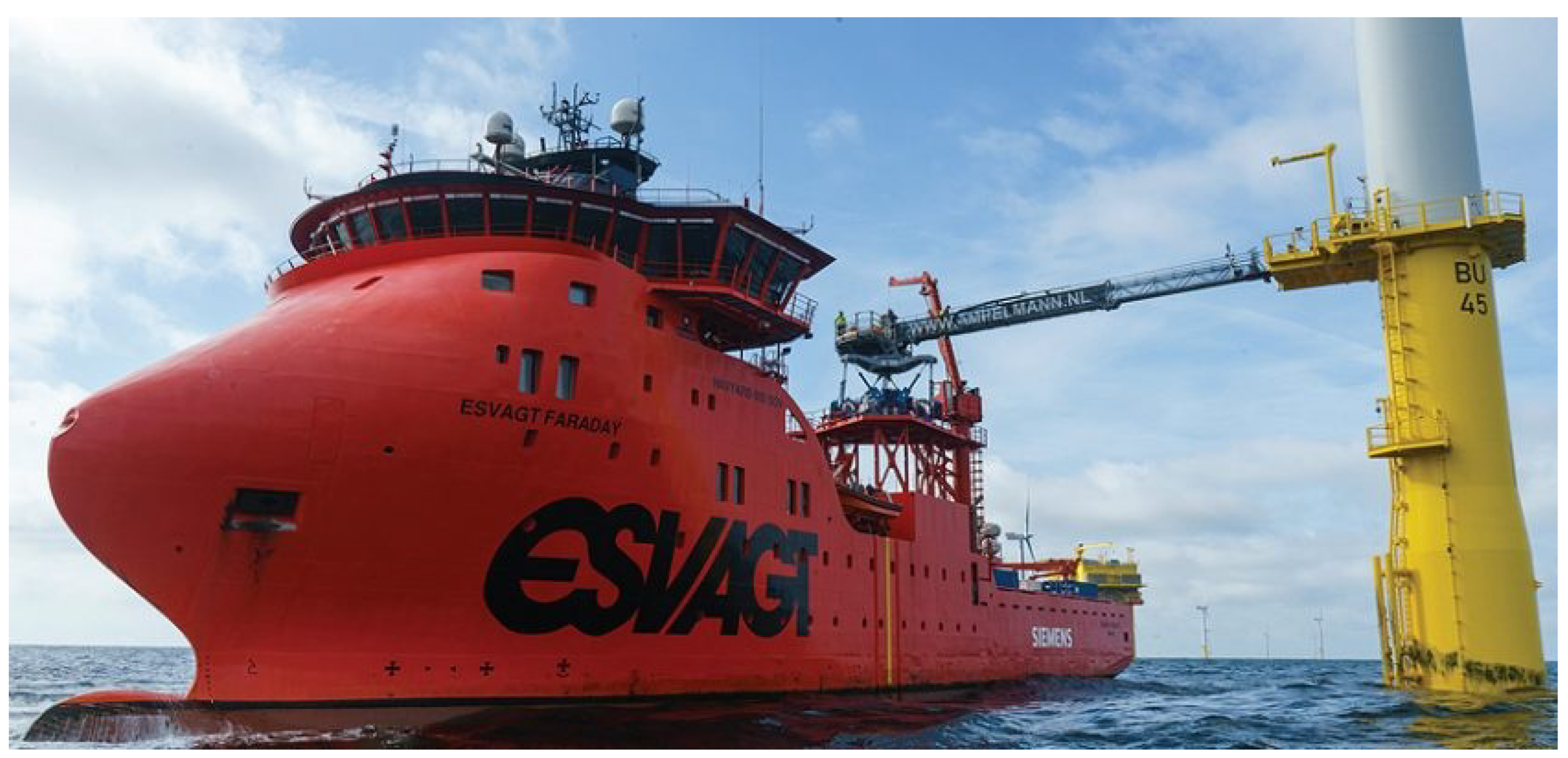
Figure 2.
Stewart platform-based motion compensated gangway. (Courtesy of Ampelmann).
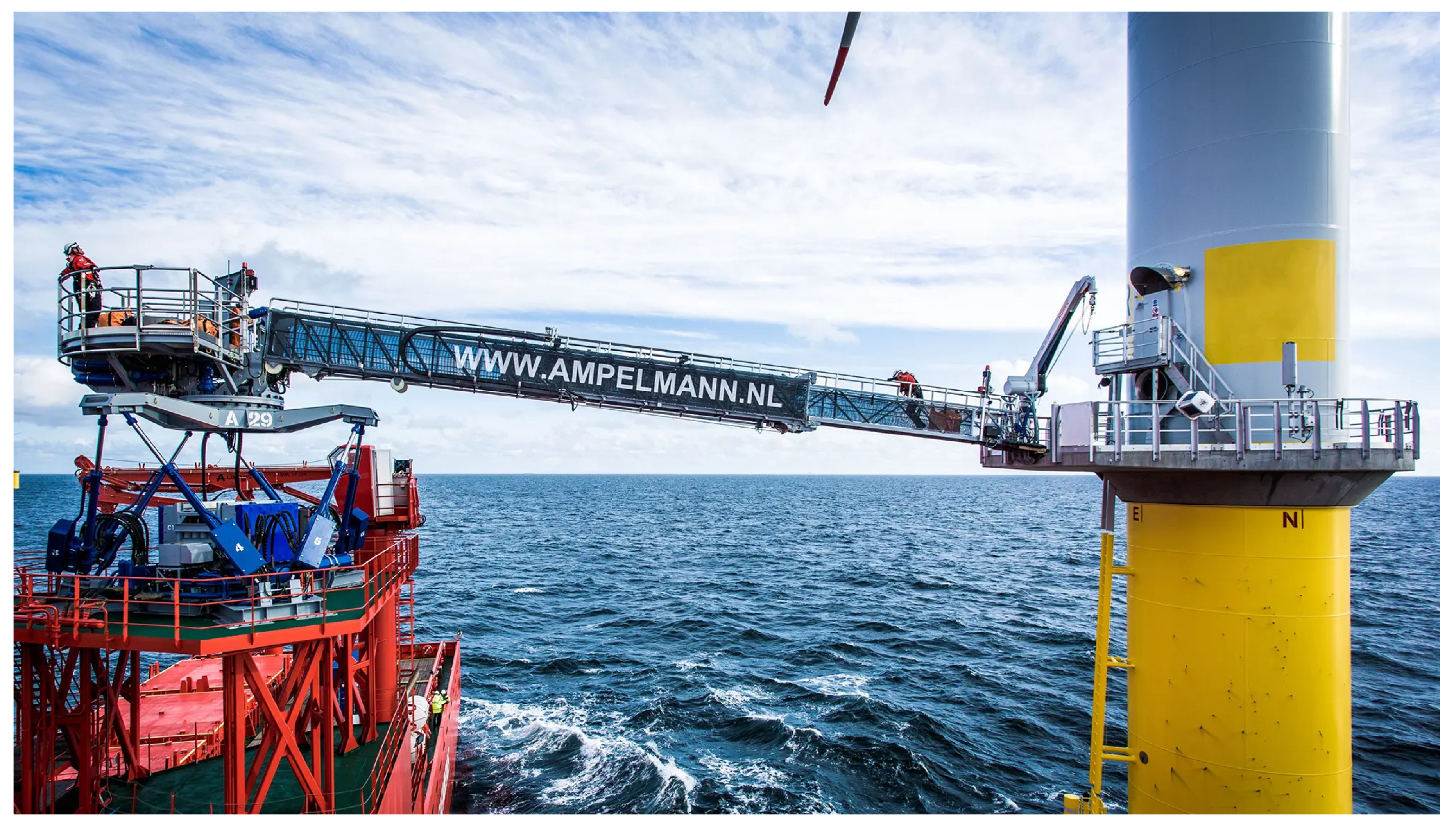
Figure 3.
Simulation and validation framework for the coupled SOV-Gangway-Turbine system.
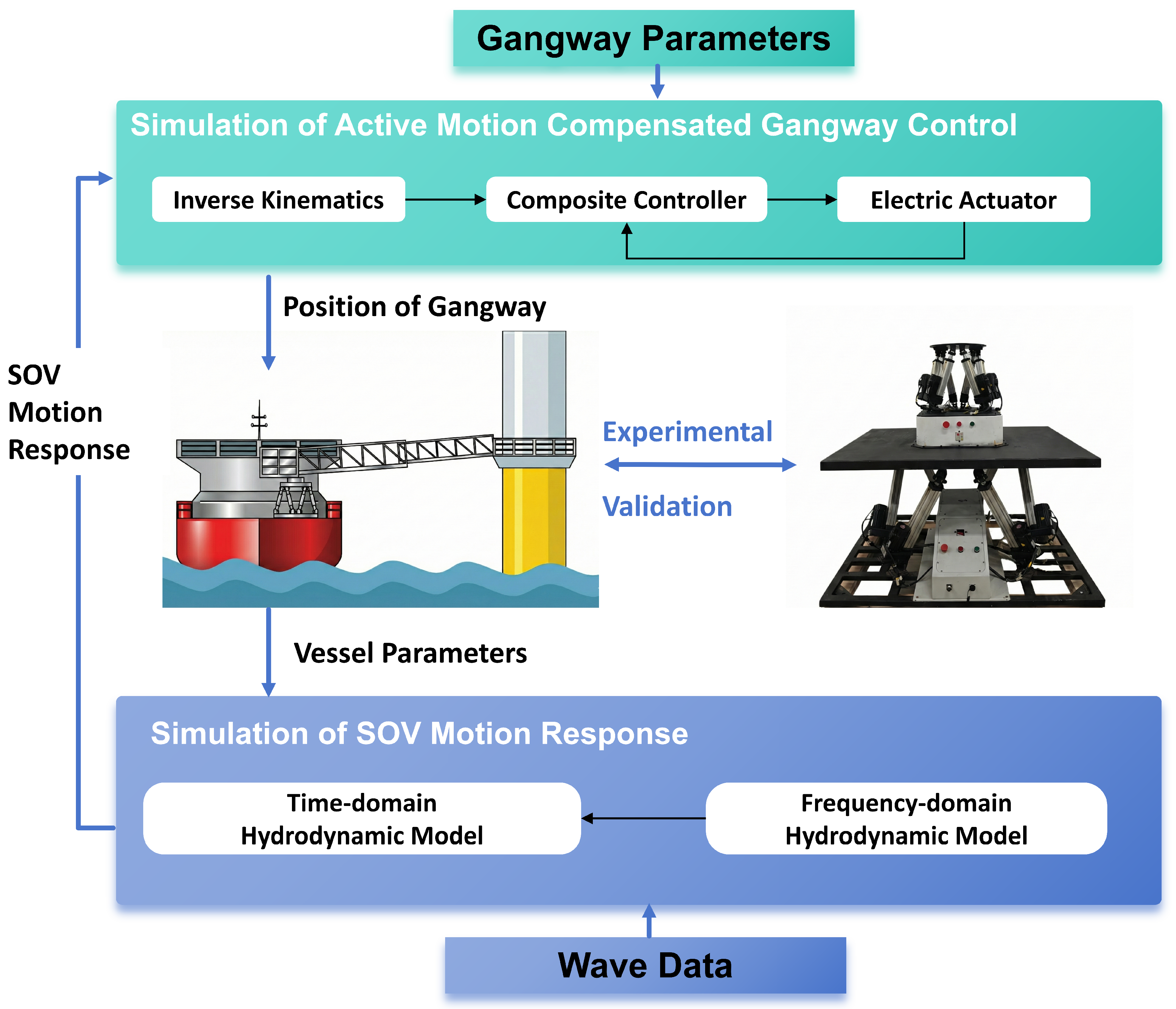
Figure 4.
The structure of the Stewart platform.
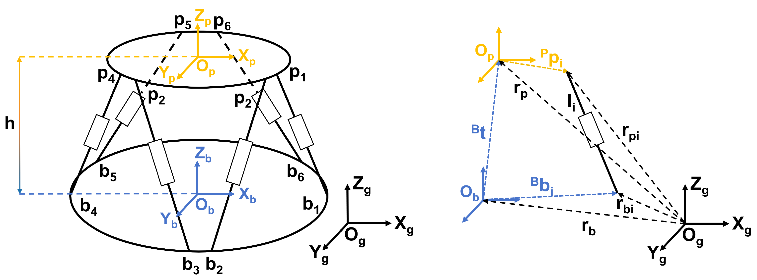
Figure 5.
Simulink control system model for Stewart platforms.

Figure 6.
Wave scatter diagram of an offshore wind farm in Guangdong.
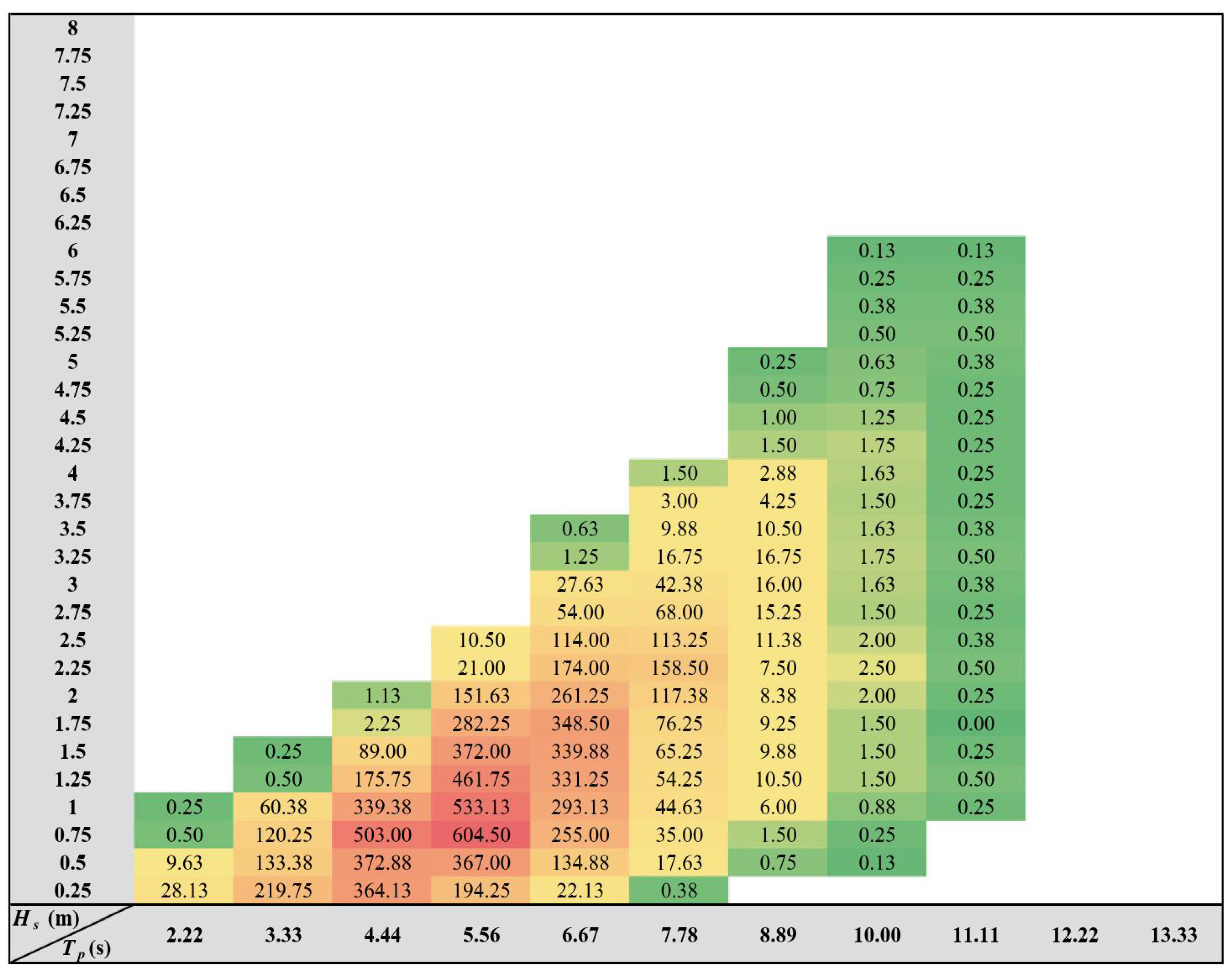
Figure 7.
JONSWAP wave spectrum.
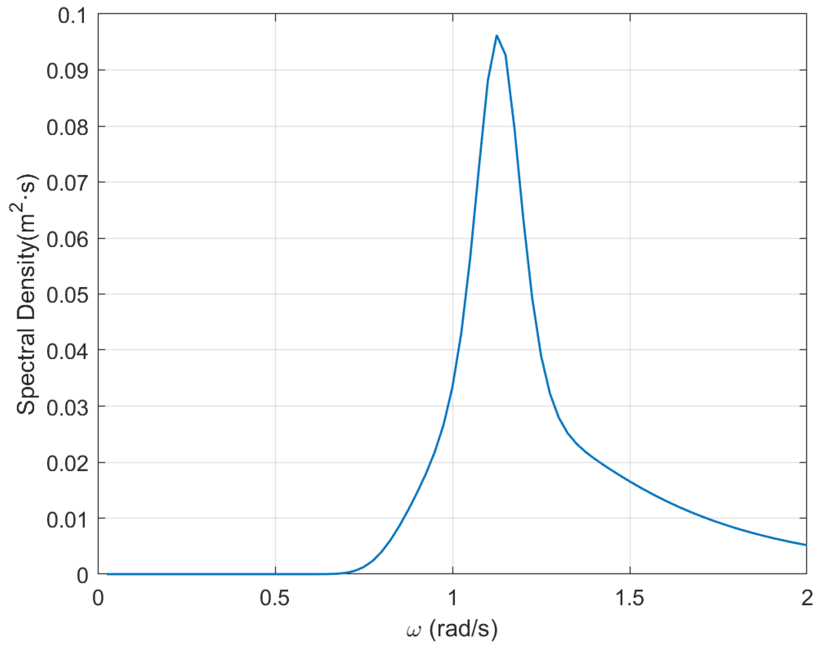
Figure 8.
Wave height time series.
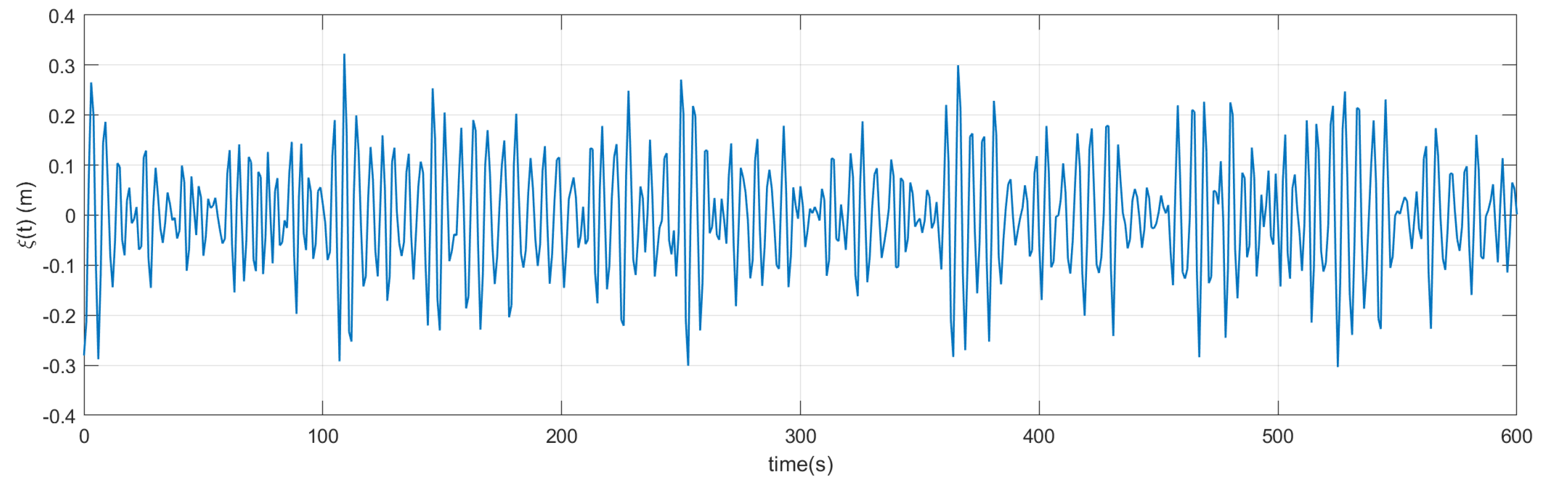
Figure 9.
Monohull service operation vessel model.
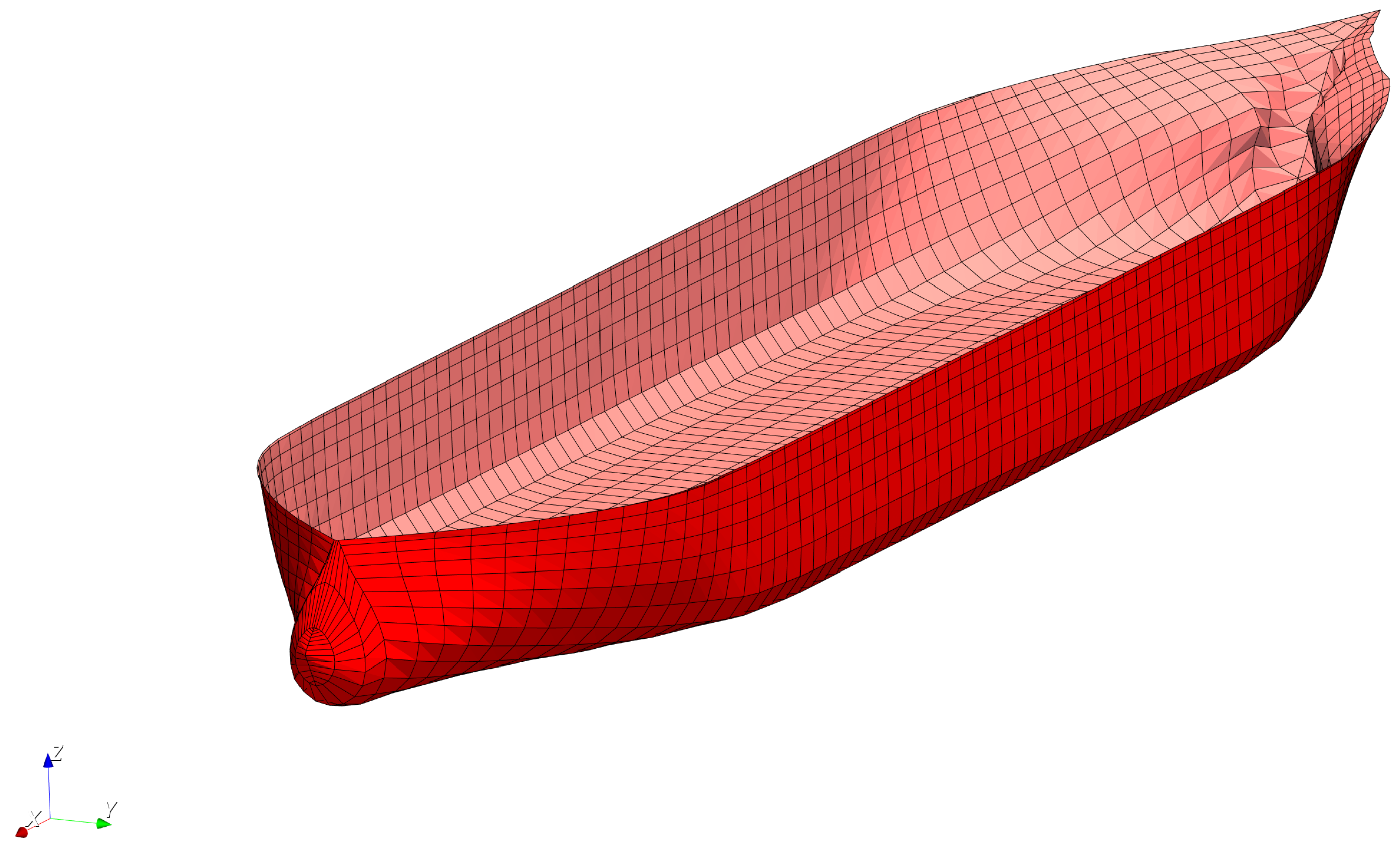
Figure 10.
Motion RAO of SOV.
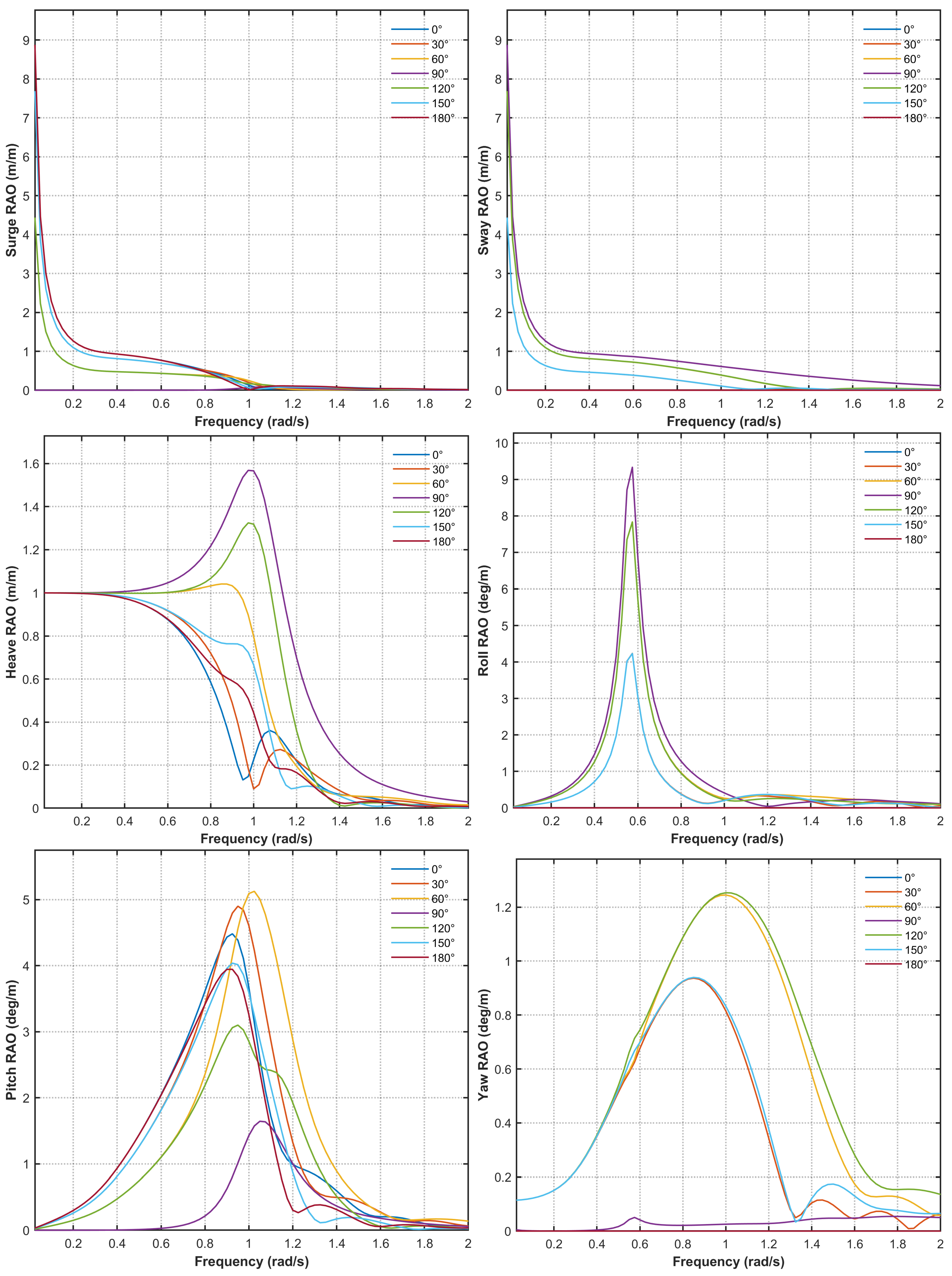
Figure 11.
The time histories of vessel’s 6-DOF responses.
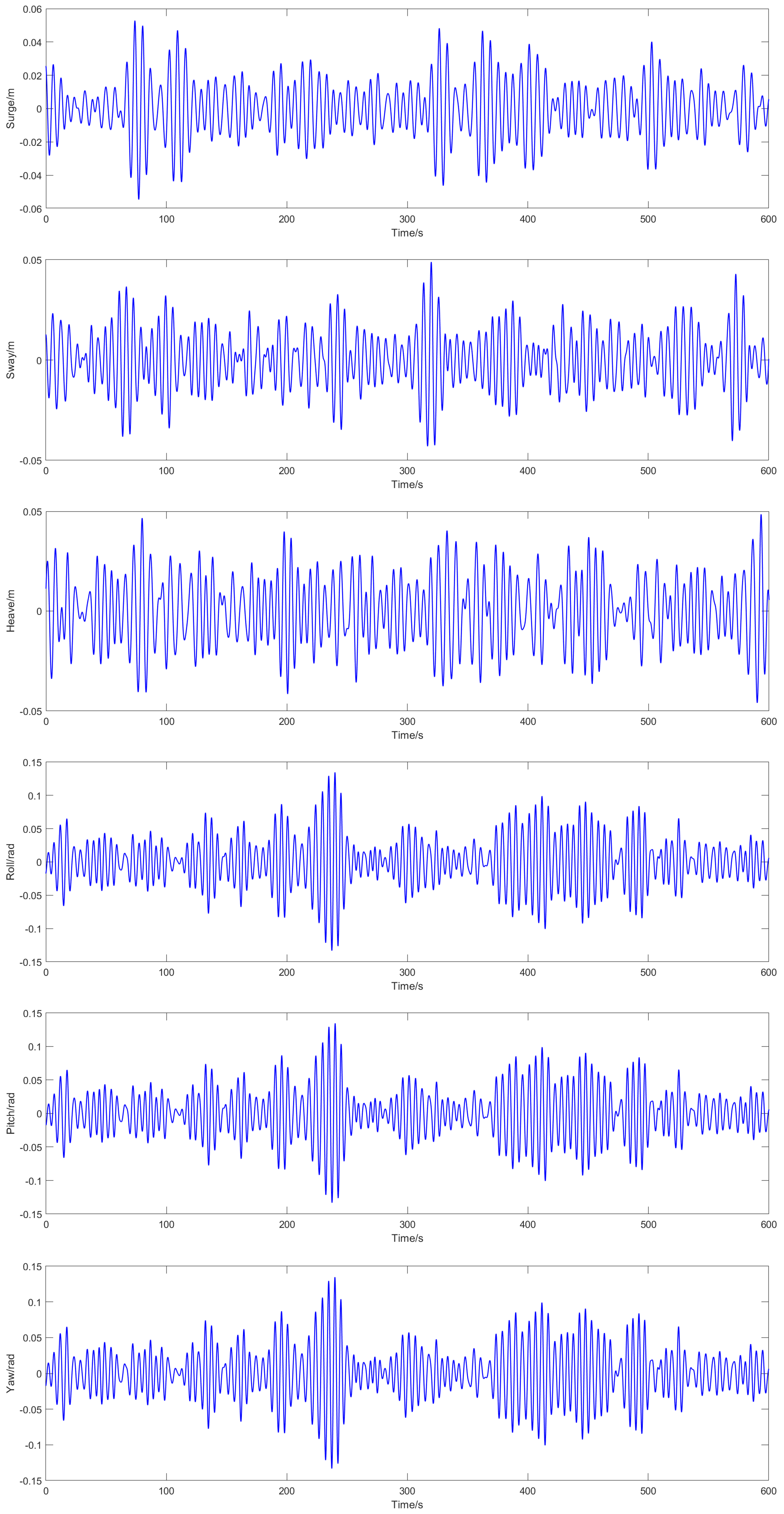
Figure 12.
The displacement of the Stewart platform’s base.
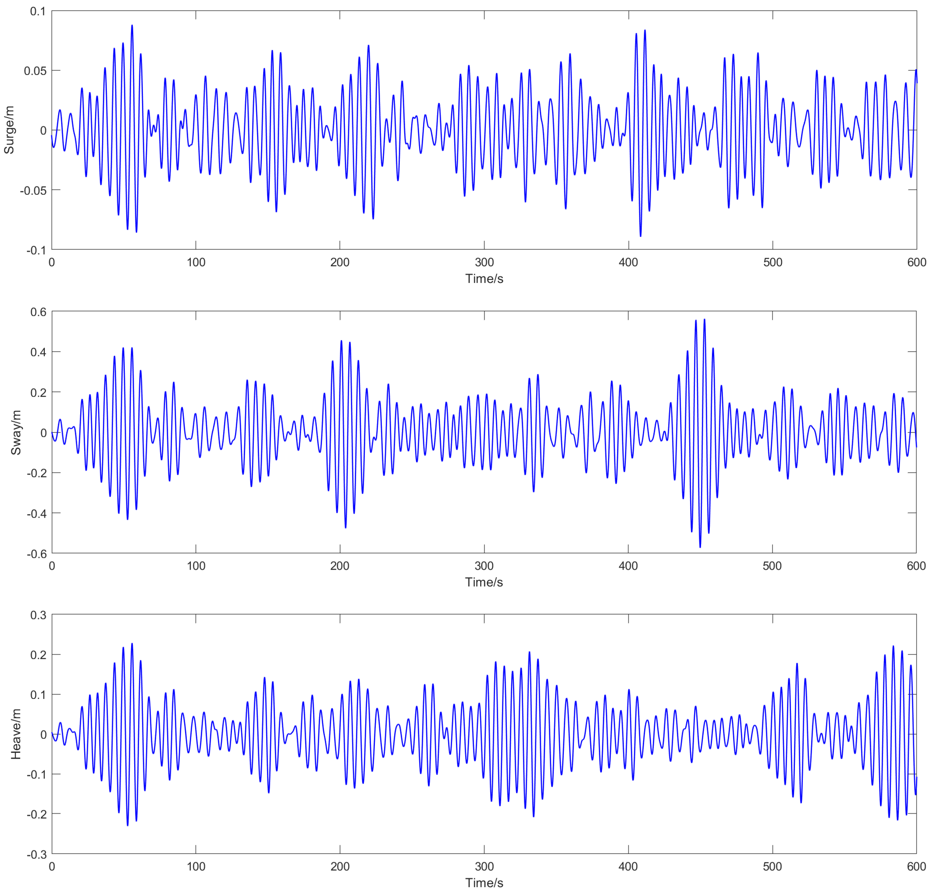
Figure 13.
Compensation amount of each leg of the Stewart platform.
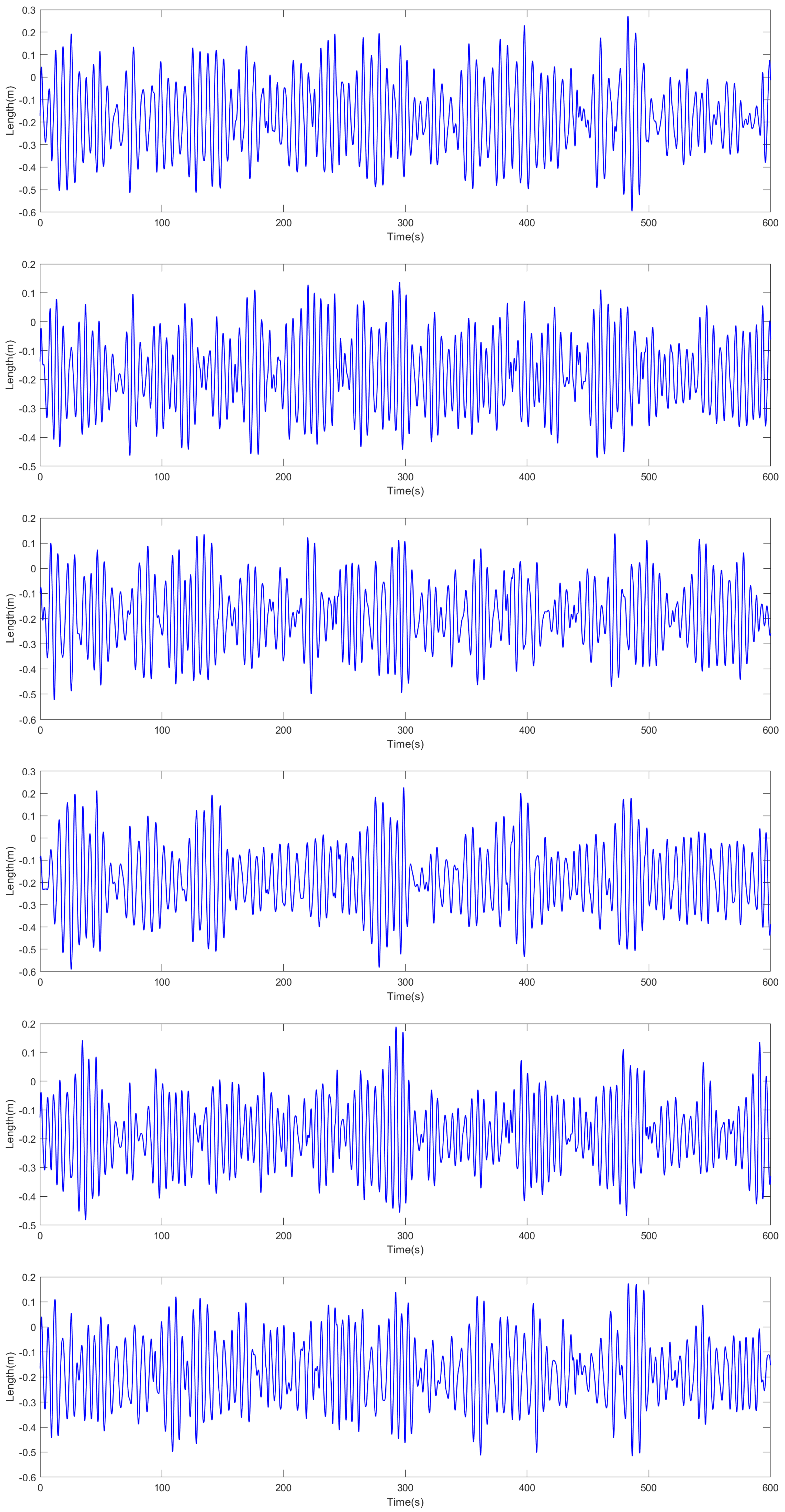
Figure 14.
6-DOF motion time history of the Stewart upper platform by using PID control.
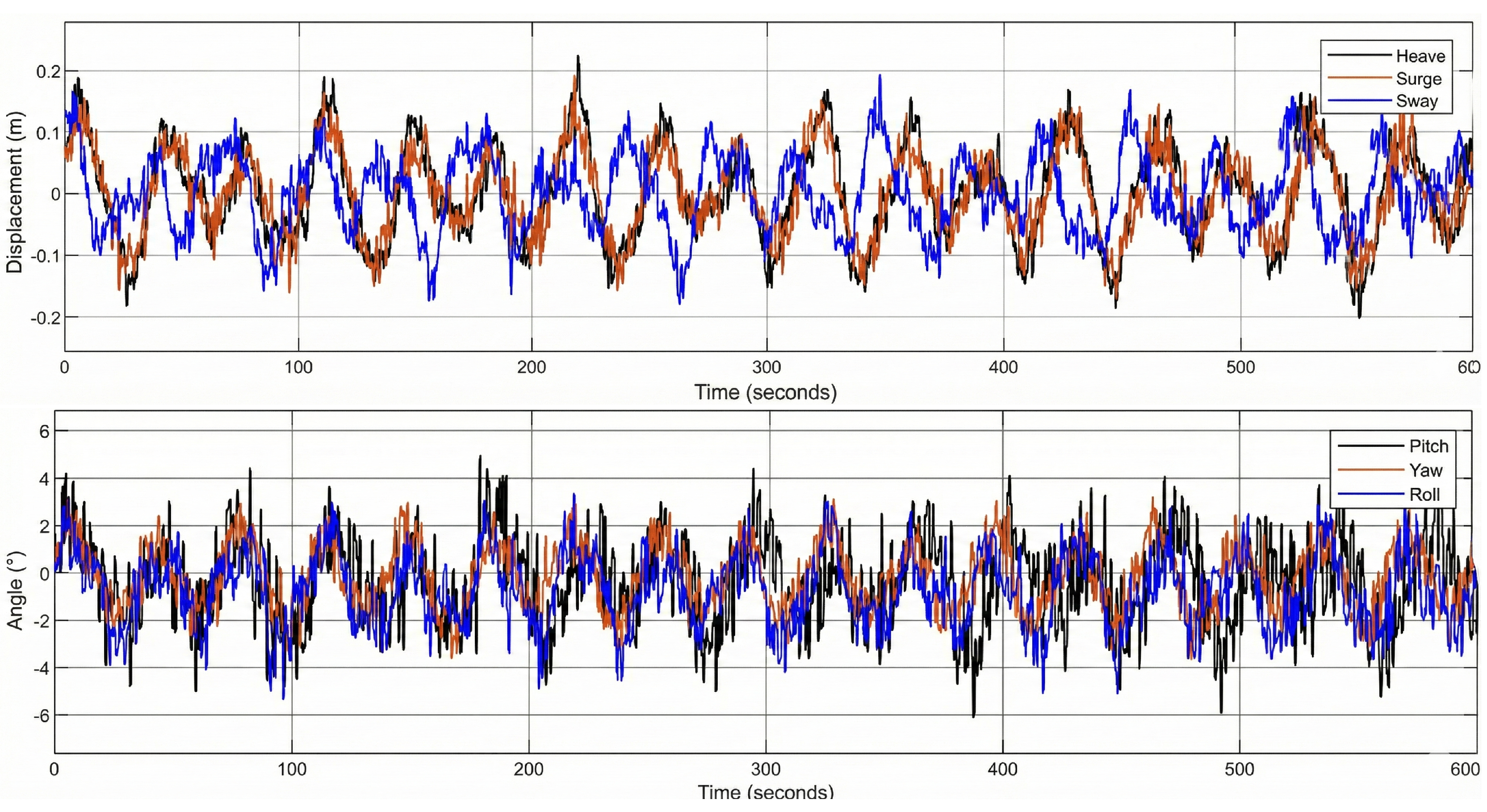
Figure 15.
Acceleration of the Stewart upper platform by using PID control.
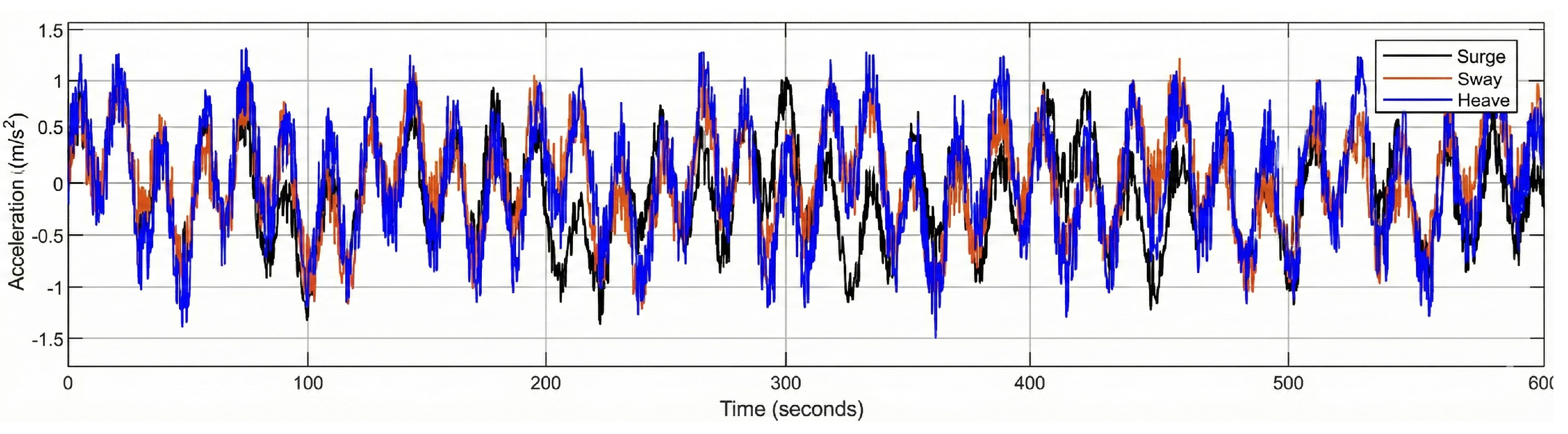
Figure 16.
6-DOF motion time history of the Stewart upper platform by composite control.
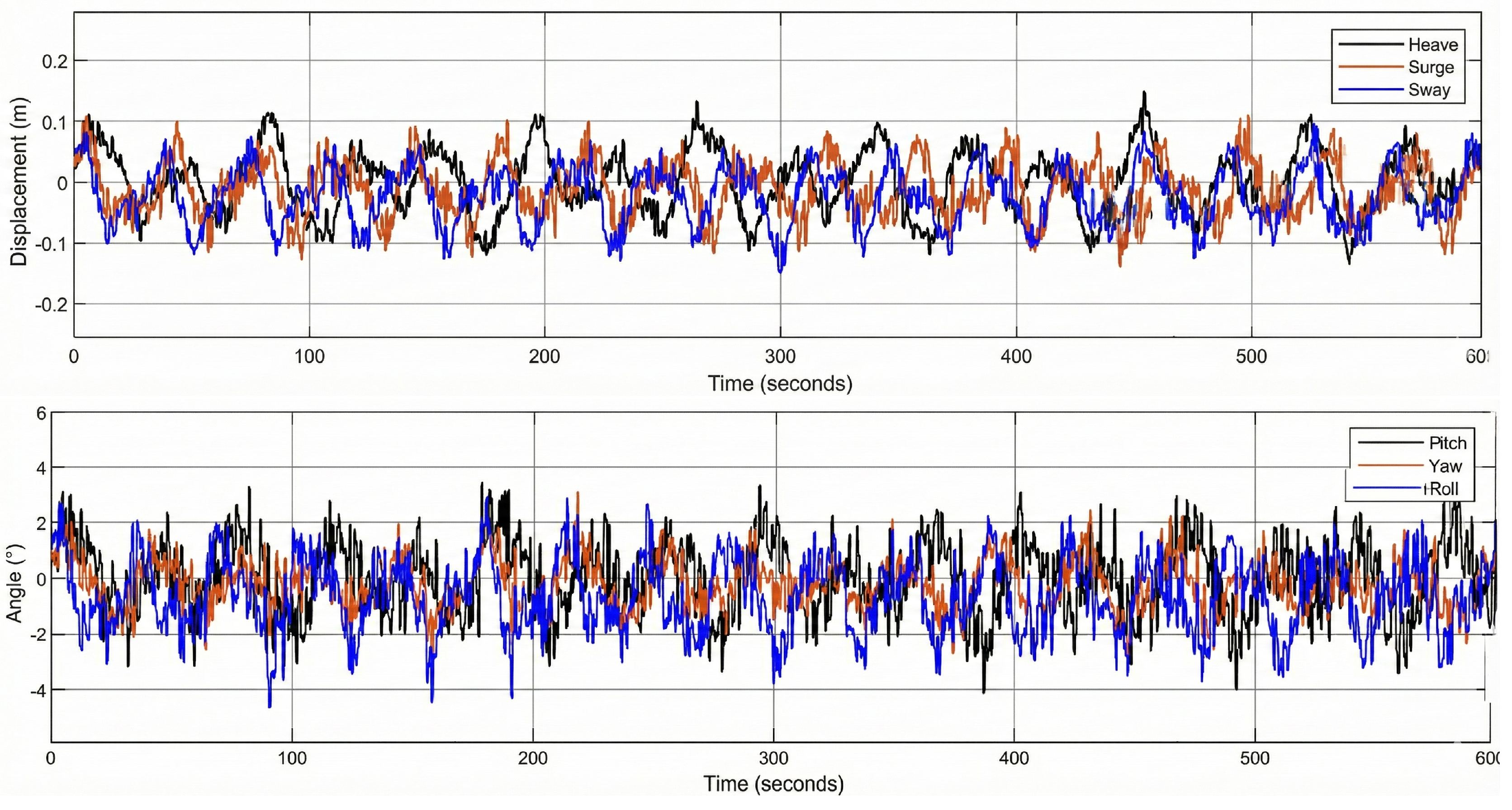
Figure 17.
Acceleration of the Stewart upper platform.
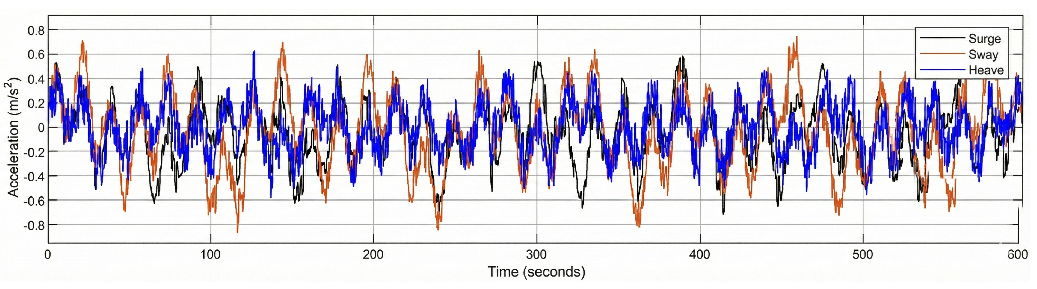
Figure 18.
Main parts of the Scaled test mechanical structure.
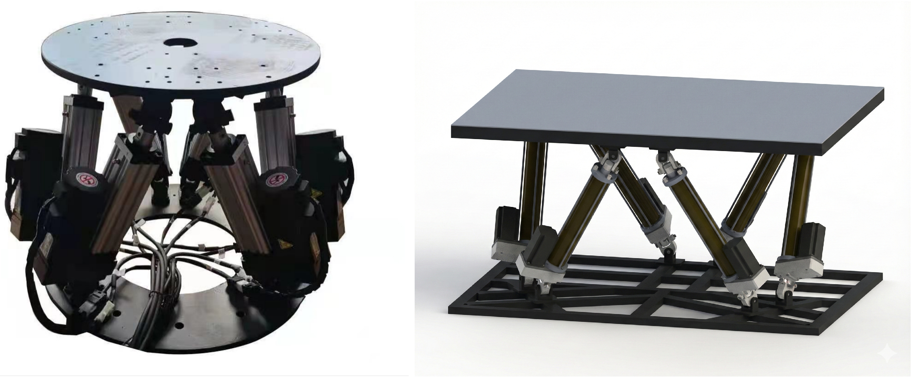
Figure 19.
Scaled test platform device for motion compensation.
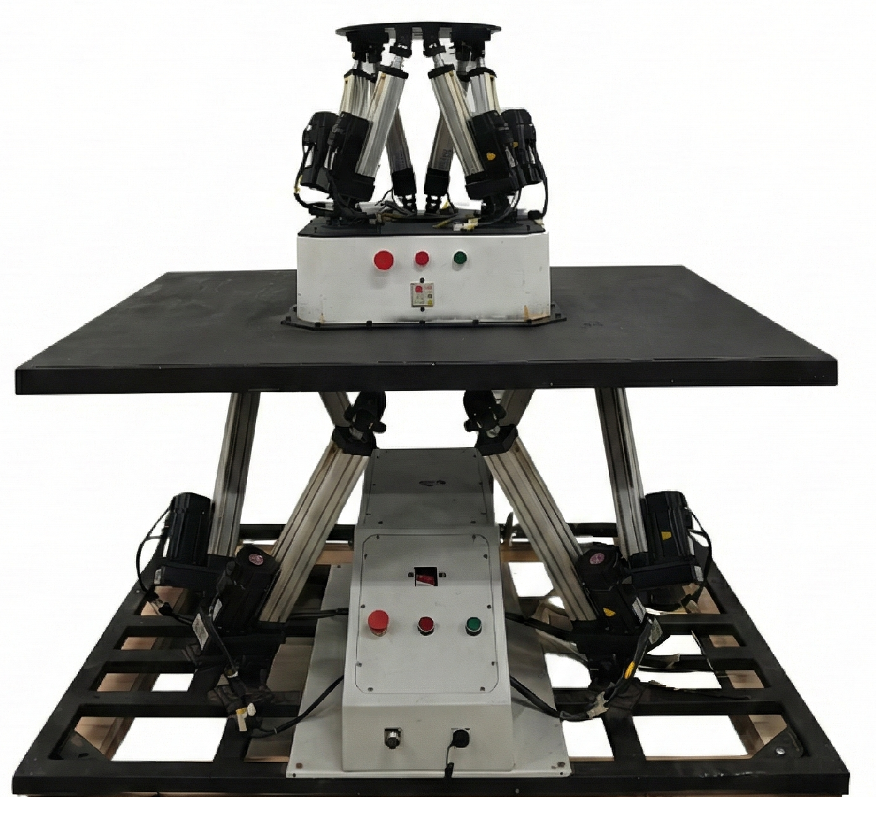
Figure 20.
Measured pose error of the compensation platform.
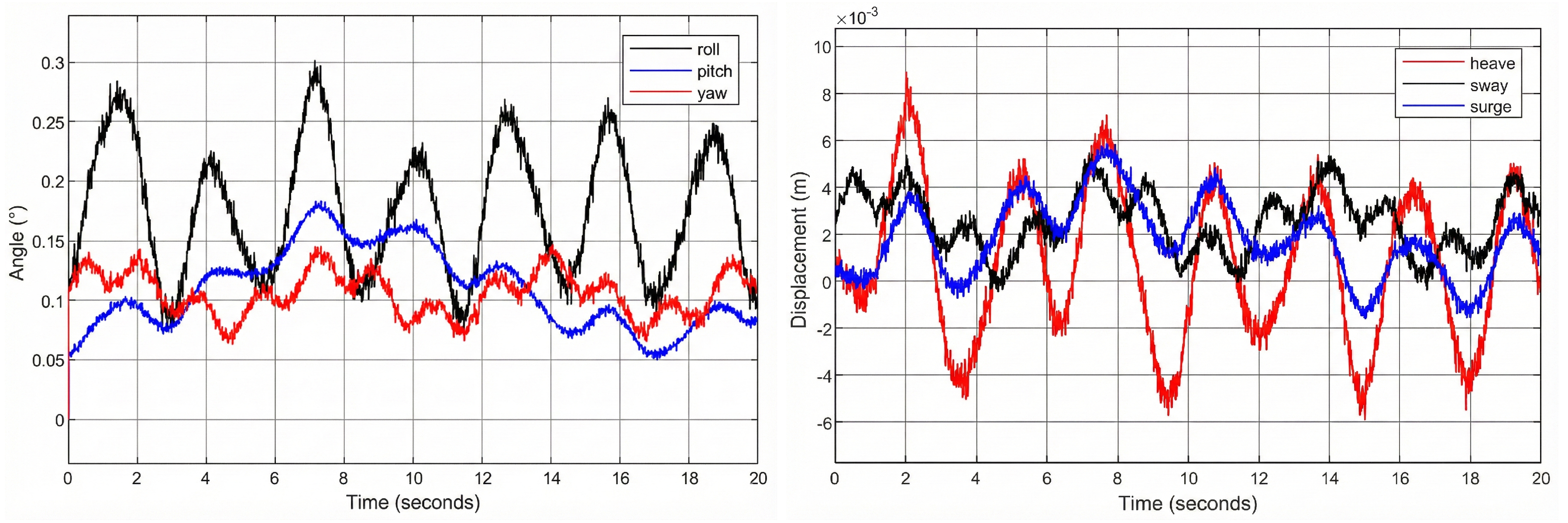
Figure 21.
The error between the model test and simulation.
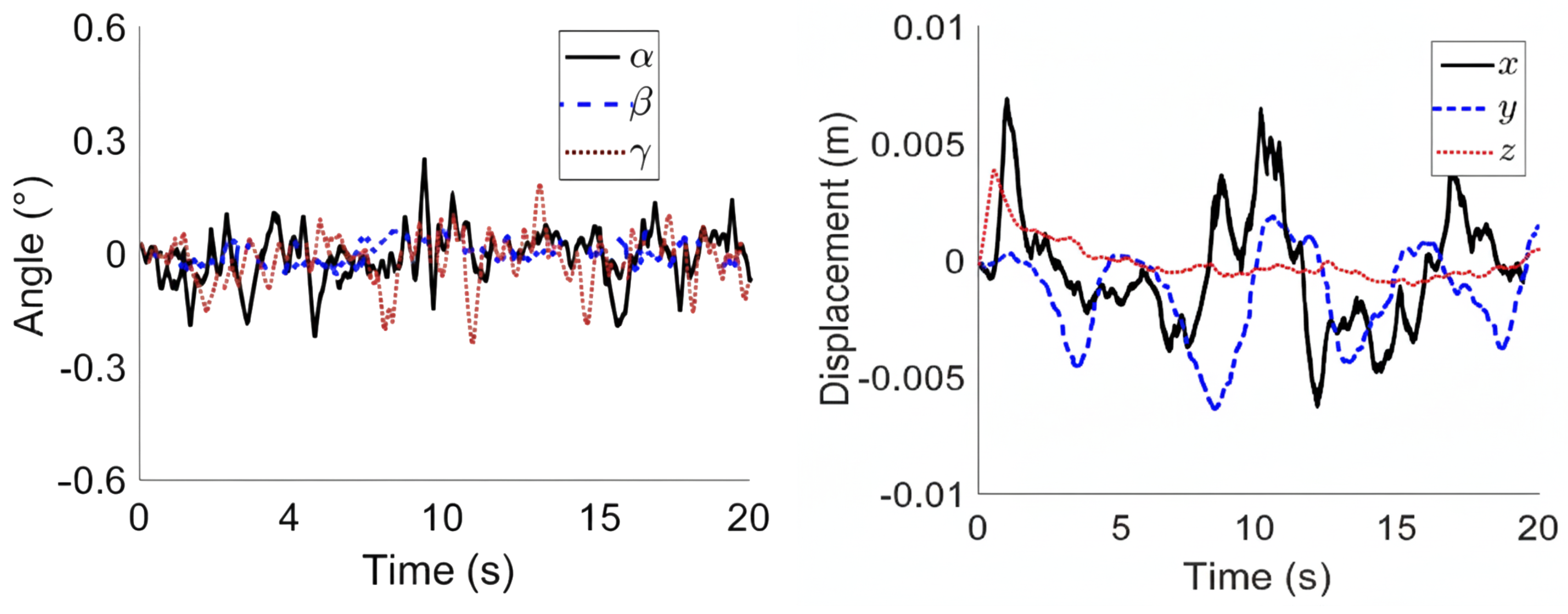
Figure 22.
,Measured pose error of the compensation platform.
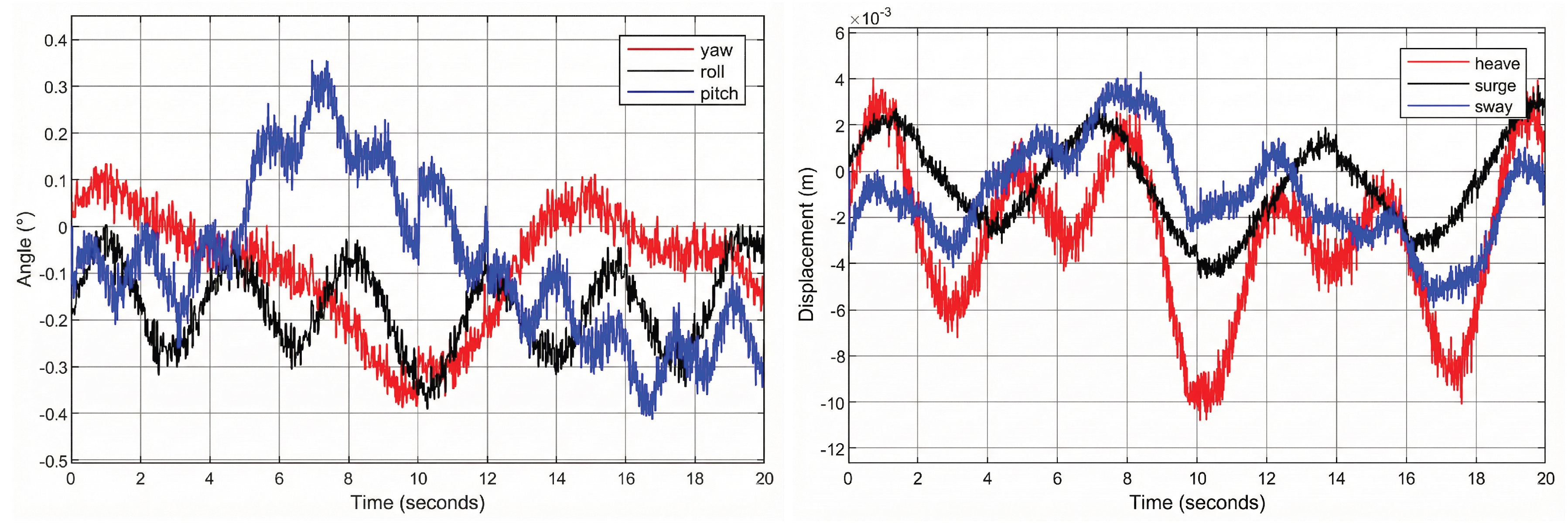
Figure 23.
The error between the model test and simulation.
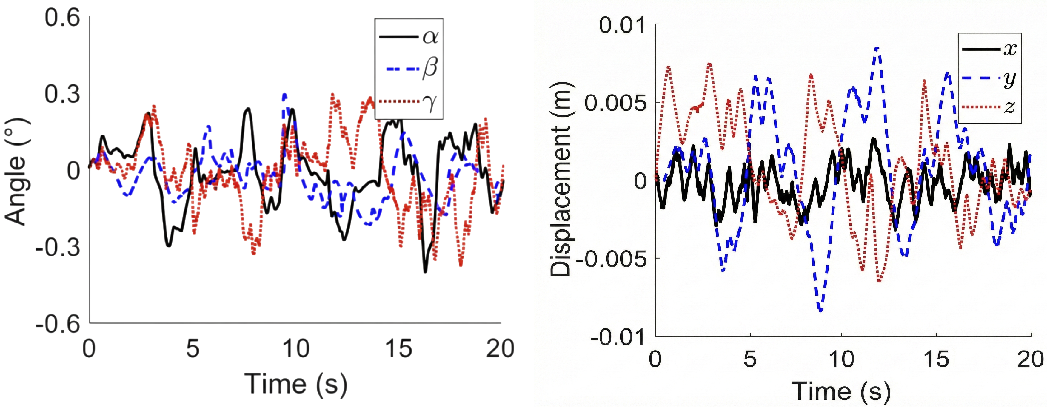
Figure 24.
,Measured pose error of the compensation platform.

Figure 25.
The error between the model test and simulation.
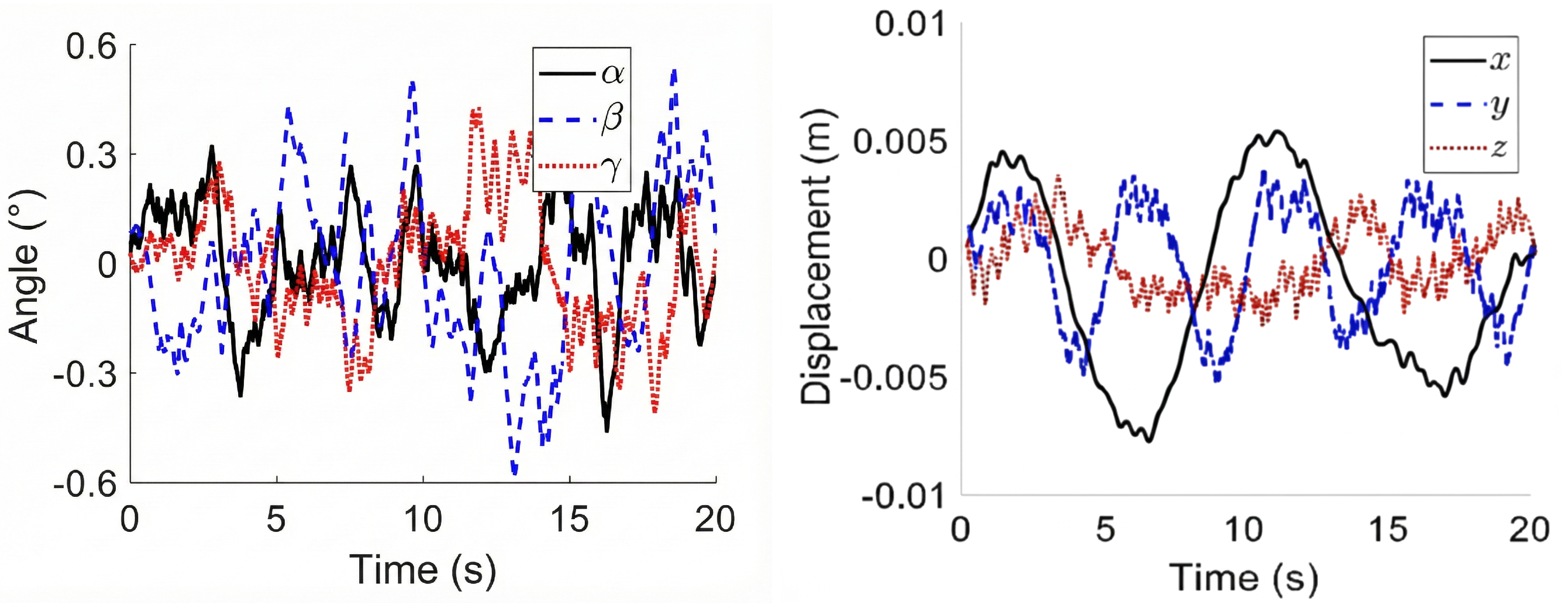

Table 1.
Mass and inertia properties of Stewart platform components.
| Component | Mass (kg) | Inertia (kg·m²) |
| Base Platform | 285.6 |
|
| Moving Platform | 163.4 |
|
| Electric Cylinder (each) | 18.3 |
|
| Gangway Load | 100.0 |
|
Table 2.
Engineering specifications of SOV.
| Item | Monohull | Unit |
| Length in overall | 66 | m |
| Breadth in overall | 15 | m |
| Mean draught in operation | 5.3 | m |
| Vertical Center of gravity (from keel) | 5.15 | m |
| Metacentric height GM | 1.05 | m |
| Displacement | 4,010 | ton |
| Roll moment of inertia | kg | |
| Pitch moment of inertia | kg | |
| Yaw moment of inertia | kg |
Table 3.
Wave compensation performance comparison.
| Degree of Freedom | PID(dB) | Composite Control (dB) |
| Heave (Z) | 17.39 | 21.58 |
| Roll () | 17.39 | 21.16 |
| Pitch () | 19.66 | 23.12 |
| Surge (X) | 17.39 | 20.93 |
| Sway (Y) | 17.39 | 20.93 |
| Yaw () | 19.66 | 23.12 |
| Average | 18.15 | 21.81 |
Table 4.
Technical specifications of the experimental platforms.
| Parameter | Motion Compensation Platform |
Ship Motion Simulator |
Unit |
| Platform Size | 1500×1200 | mm | |
| Payload Capacity | 80 | 500 | kg |
| Tilt Range | ±30 | ±15 | ° |
| Yaw Range | ±35 | ±20 | ° |
| Stroke | 160 | 100 | mm |
| Max. Velocity | 0.5 | 0.5 | m/s |
| Motor Power | 400×6 | 1000×6 | W |
| Rated Speed | 3000 | 3000 | rpm |
Table 5.
Wave conditions parameters.
| Parameter | Case1 | Case2 | Case3 | Unit |
| Significant wave height | 0.75 | 1 | 0.75 | m |
| Peak period | 5.56 | 5.56 | 4.44 | s |
Disclaimer/Publisher’s Note: The statements, opinions and data contained in all publications are solely those of the individual author(s) and contributor(s) and not of MDPI and/or the editor(s). MDPI and/or the editor(s) disclaim responsibility for any injury to people or property resulting from any ideas, methods, instructions or products referred to in the content. |
© 2025 by the authors. Licensee MDPI, Basel, Switzerland. This article is an open access article distributed under the terms and conditions of the Creative Commons Attribution (CC BY) license (http://creativecommons.org/licenses/by/4.0/).
Copyright: This open access article is published under a Creative Commons CC BY 4.0 license, which permit the free download, distribution, and reuse, provided that the author and preprint are cited in any reuse.


