
Submitted:
16 December 2025
Posted:
18 December 2025
You are already at the latest version
Abstract
The increasing demand for sustainable energy production necessitates the development of innovative technologies for converting municipal waste into valuable energy offering a viable alternative to fossil fuels. This study presents a flexible, portable, and expandable waste-to-energy concept that integrates gasification and pyrolysis processes production of combustible gases and liquid fuels. Particular emphasis is placed on the use of transparent and interpretable modeling approaches to support system optimization and future scalability. The proposed methodology is demonstrated on two experimental systems currently operated at CEET Explorer, VSB – Technical University of Ostrava, Czech Republic: (i) a primary gasification facility equipped with a plasma torch, reactor, hydrogen separator and tank, fuel cells, and renewable grid connections; and (ii) a secondary pyrolysis unit designed to maximize pyrolysis oil production. Both systems are modeled and simulated using in-house software developed in Python, employing stoichiometric balances, symbolic regression, and polynomial regression to represent chemical reactions and energy flows. The findings demonstrate that transparent models—such as stoichiometric modeling combined with interpretable machine learning—can accurately reproduce the operational behavior of waste-to-energy processes. Gasification is optimized for hydrogen generation and electricity production via fuel cells, whereas pyrolysis favors liquid fuel yield with syngas as a by-product. Molar mass relations are applied to ensure consistent conversion between mass and volume across gasification, pyrolysis, and combustion pathways, maintaining the conservation of mass. Overall, the integration of stoichiometric balance models with symbolic and polynomial regression provides a reliable and interpretable framework for simulating real waste-to-energy systems. The current results, based on bio-wood waste from the Czech Republic, validate the proposed methodology, which is made openly available to promote transparency, reproducibility, and further advancement of sustainable waste-to-energy technologies.
Keywords:
1. Introduction
1.1. Background
1.2. Literature Overview
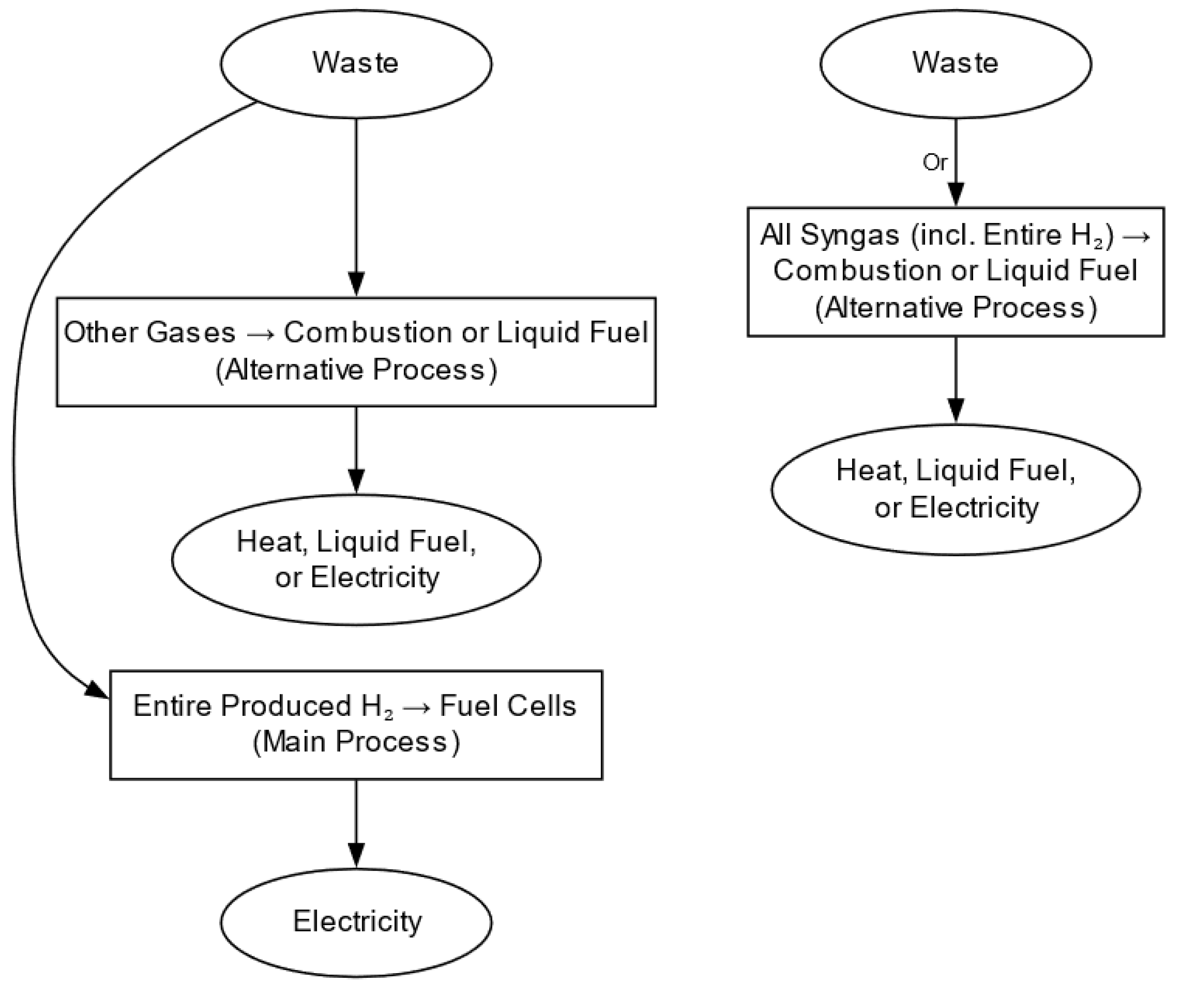
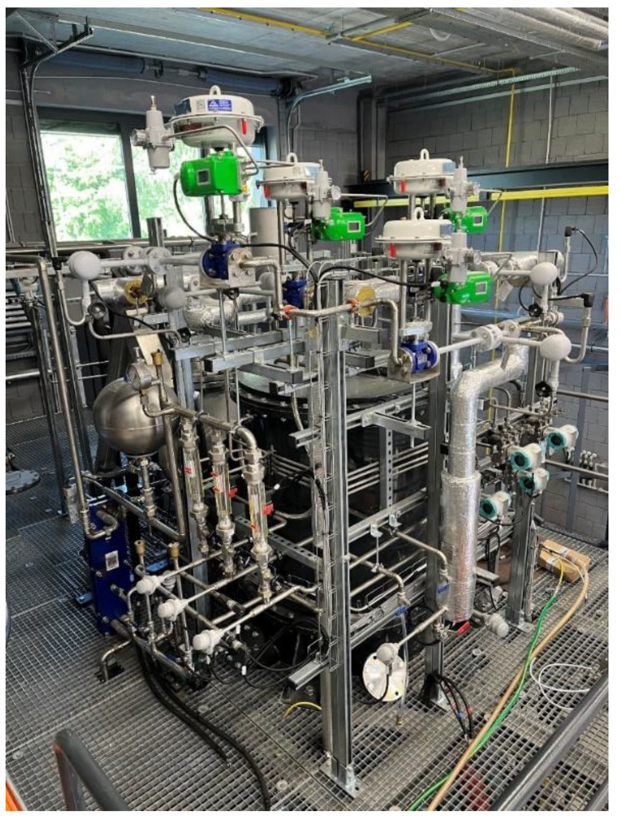
2. Waste-to-Energy Experimental Facilities — Models of the System
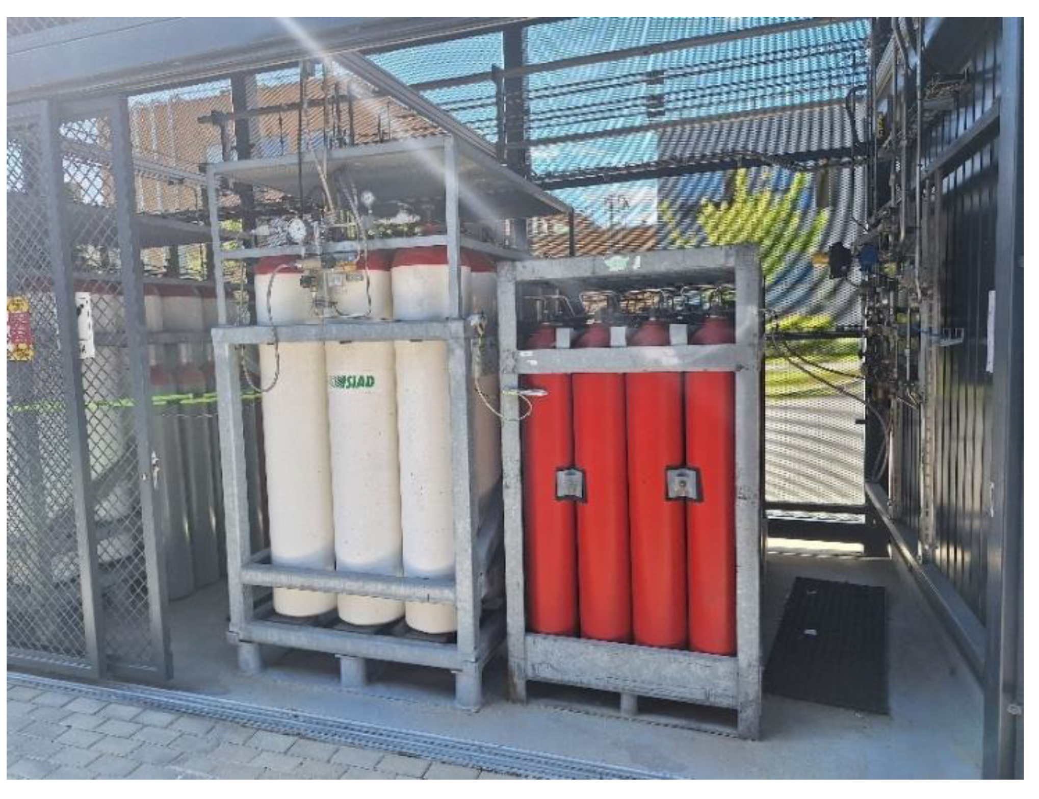
2.1. Gasification Facility – Primary Facility of the Observed Waste-to-Energy System
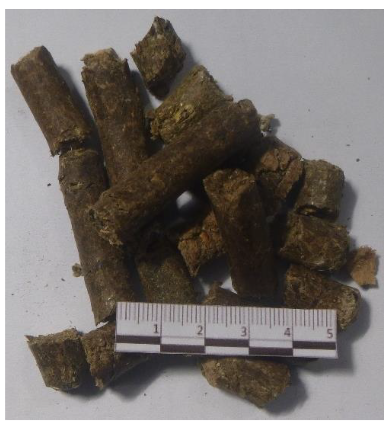
2.1.1. Alternative Fuel
2.1.2. Plasma Torch
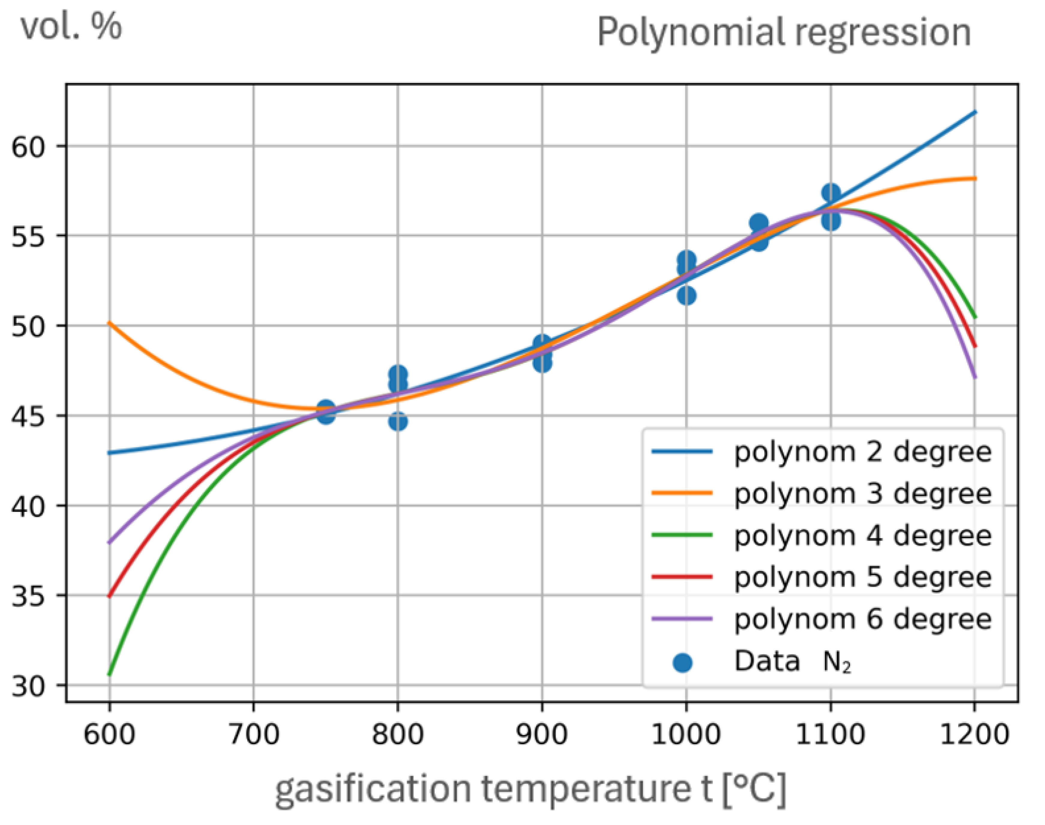
2.1.3. Gasification Reactor - Amount and Composition of Syngas Based on Temperature
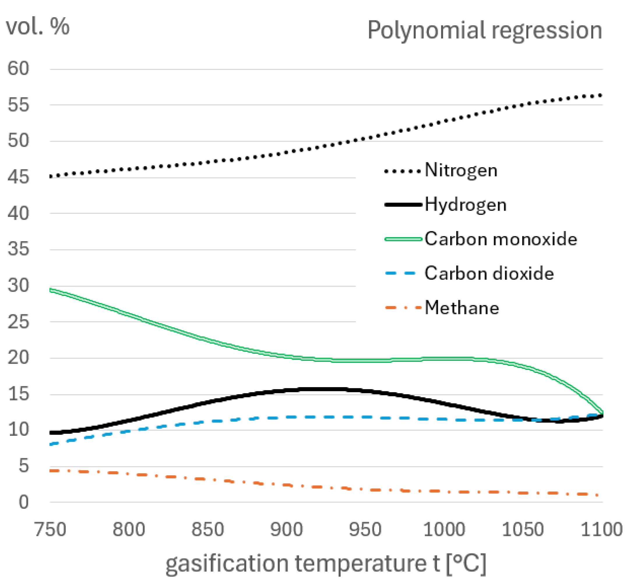
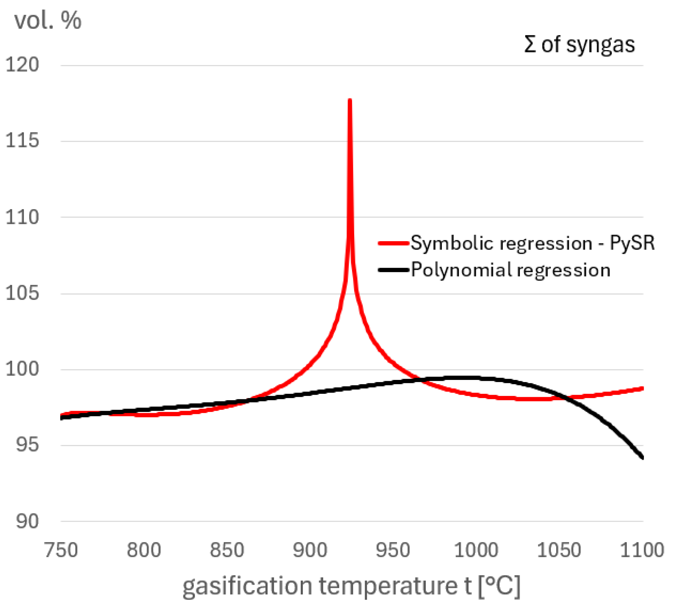
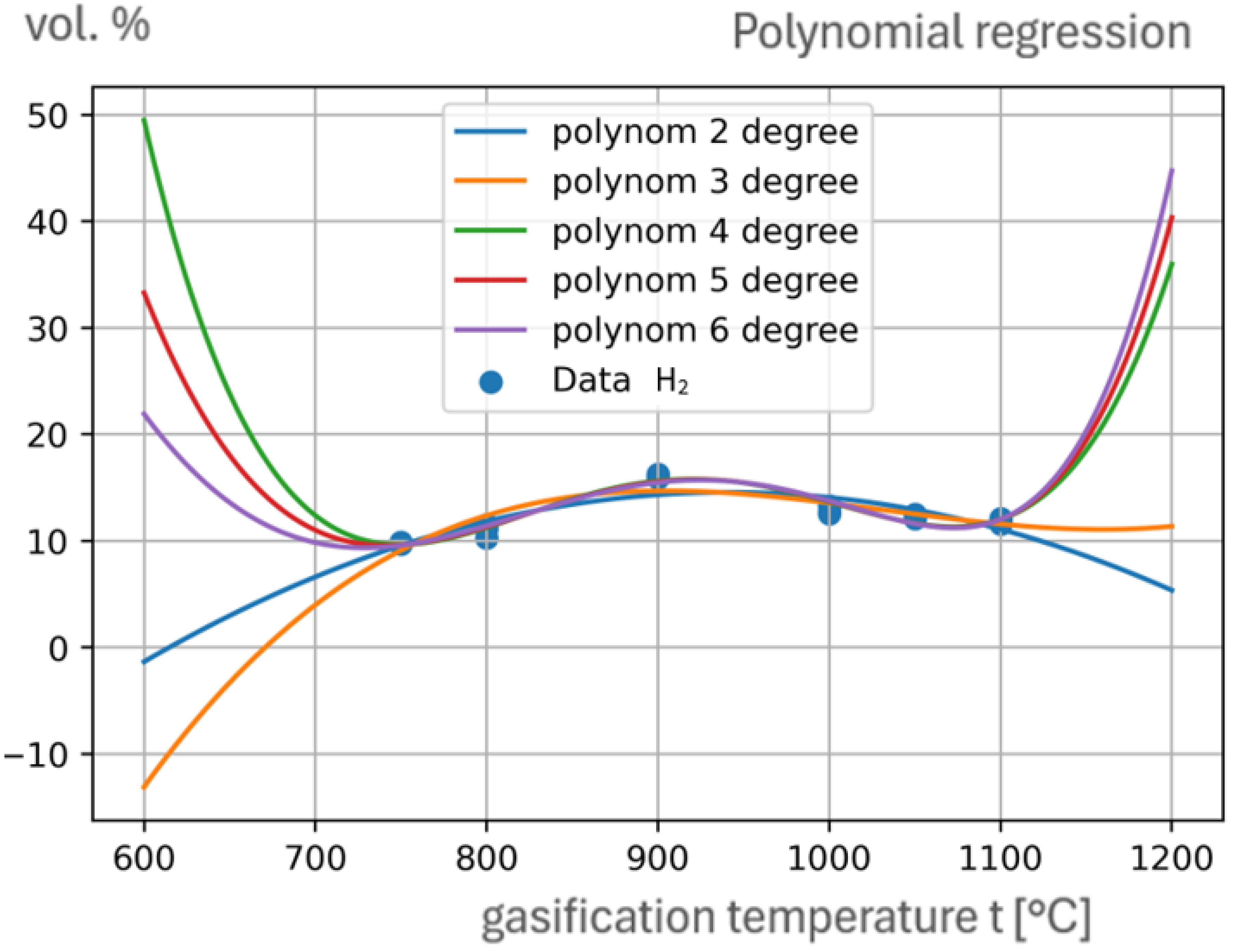
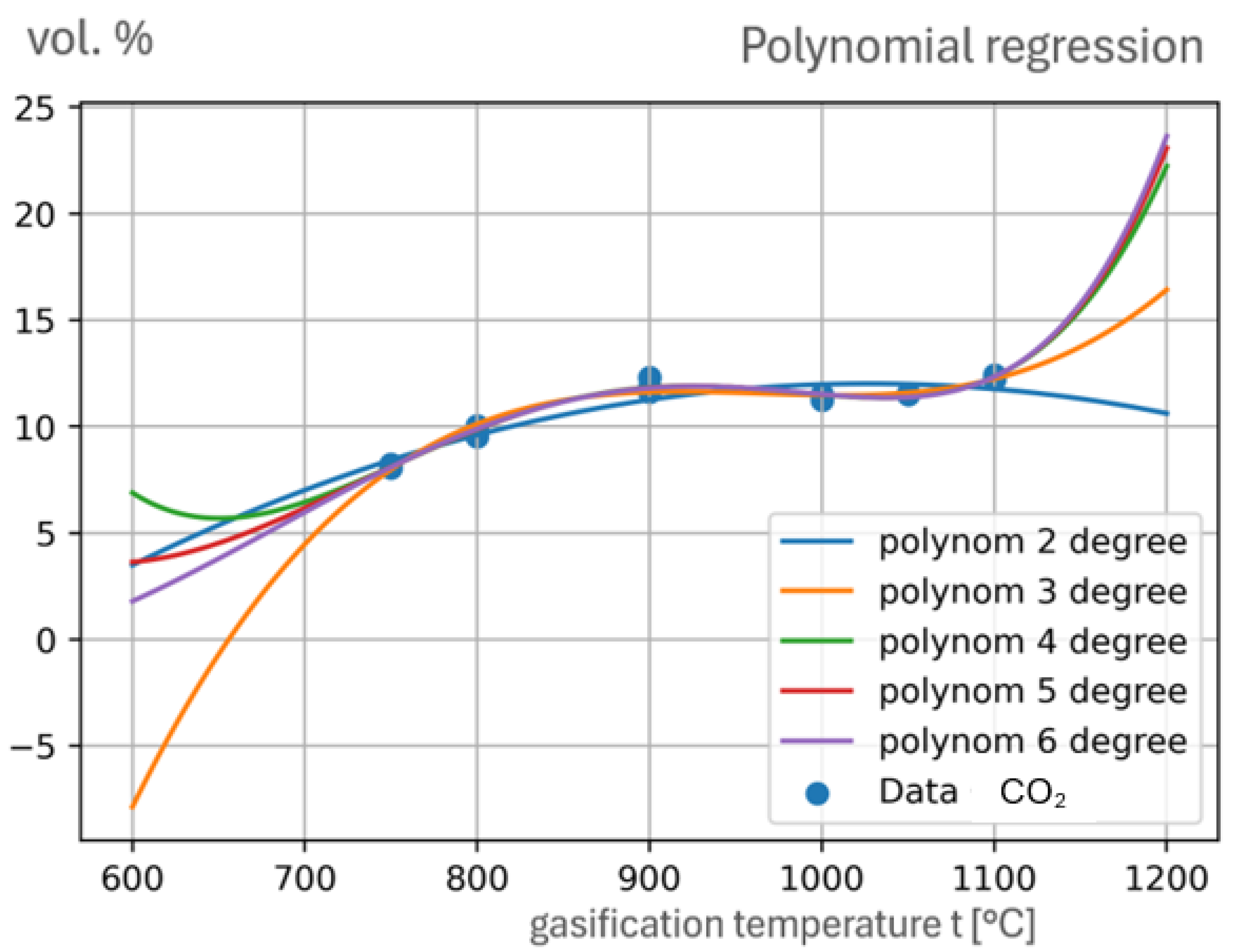
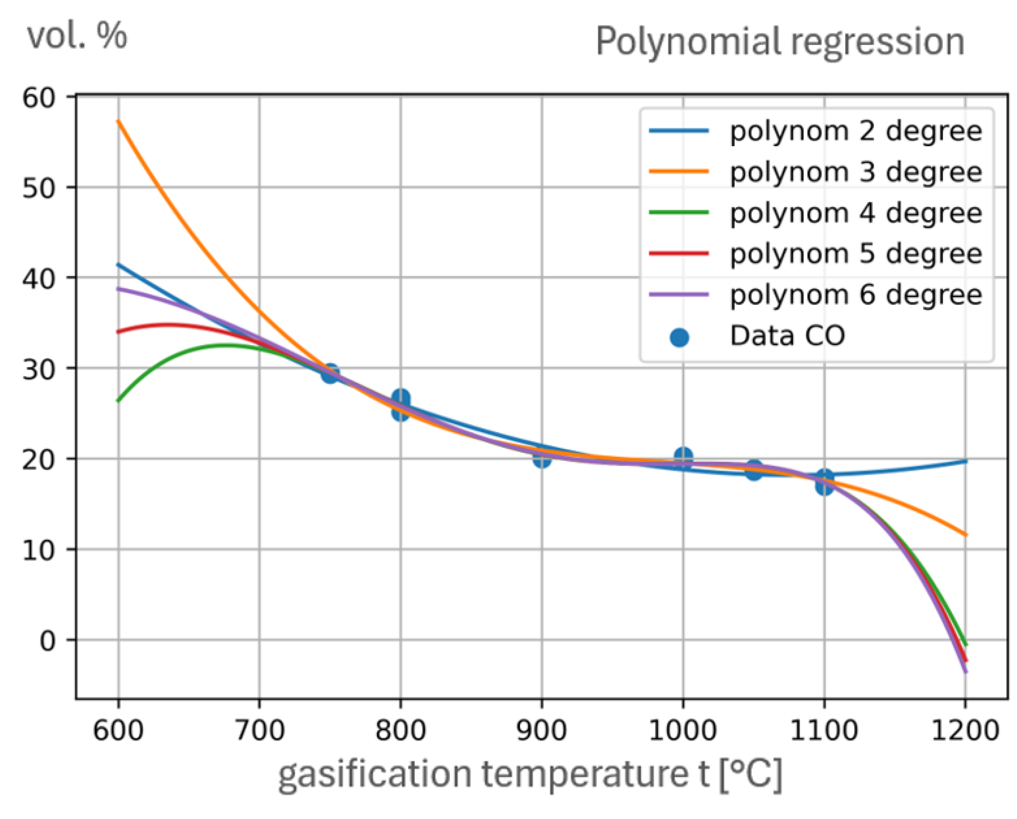
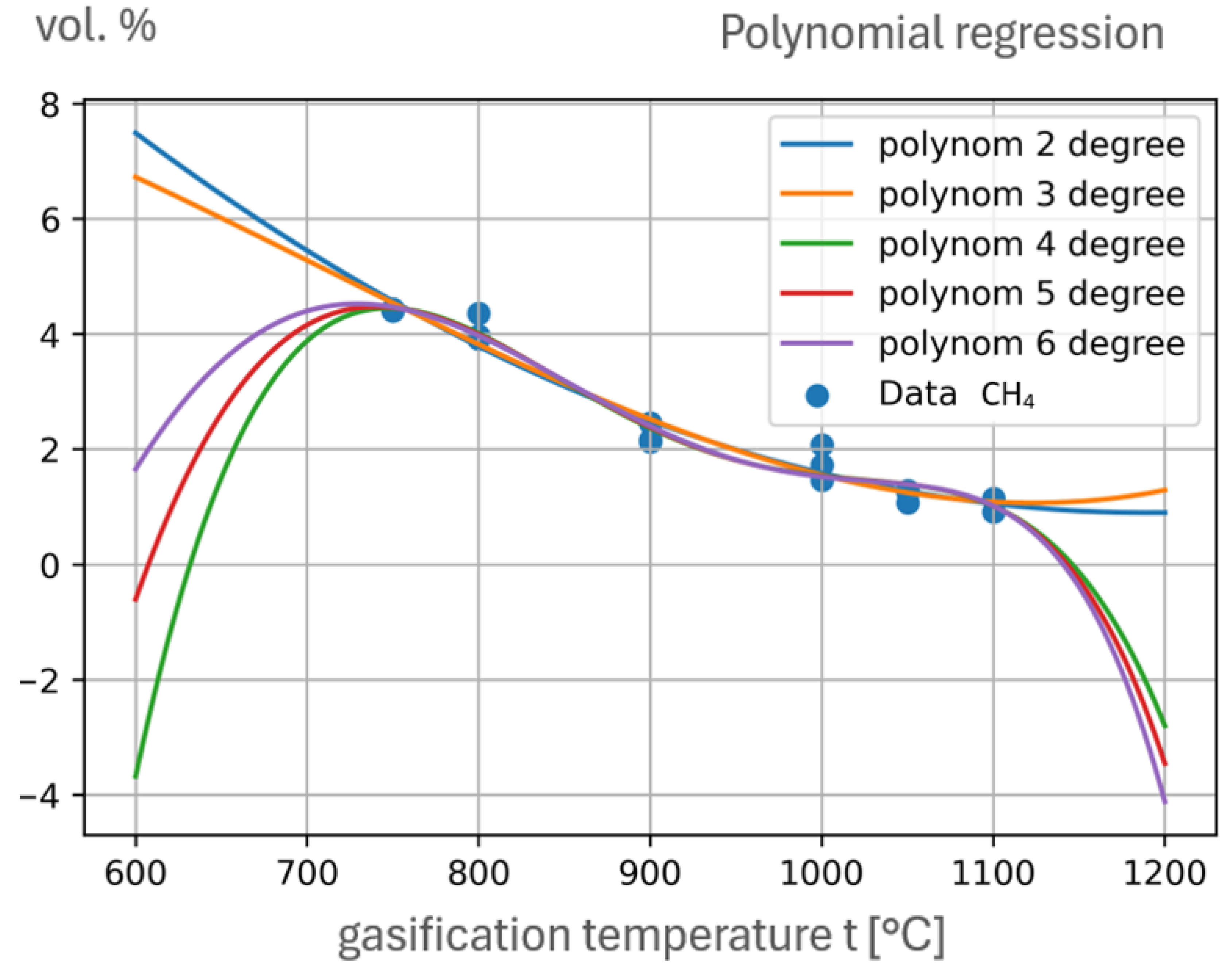
- Polynomial regression: For the middle temperature in the gasification reactor t ranging from 879 °C and 966 °C, the production of hydrogen is maximal with an amount larger than 15% and never reaches 16%. The absolute peak for the production of H2 is for t=923 °C. For t=923 °C, CO2 11.87 %, CO 19.76 %, CH4 2.11 %, and N2 49.3 %, which gives a total of 98.78 % while the rest are other gases.
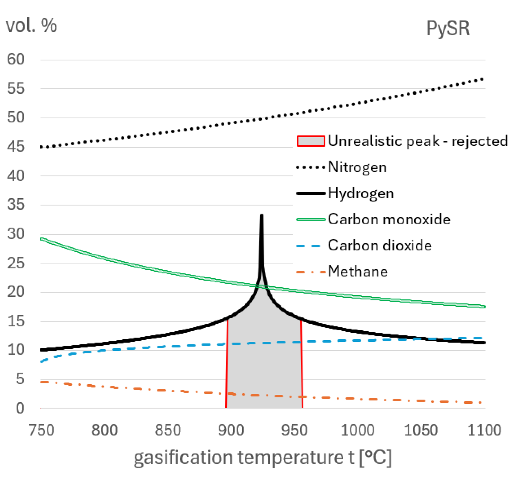
- Symbolic regression – PySR: A model for all components of syngas can be used except for hydrogen, for which polynomial regression formulation should be used instead.
- Hydrogen H2
- Carbon dioxide CO2
- Carbon monoxide CO
- Methane CH4
- NitrogenN2
2.1.4. Hydrogen Separation
2.1.5. Hydrogen Tank
2.1.6. Fuel Cells and Electrolyzers
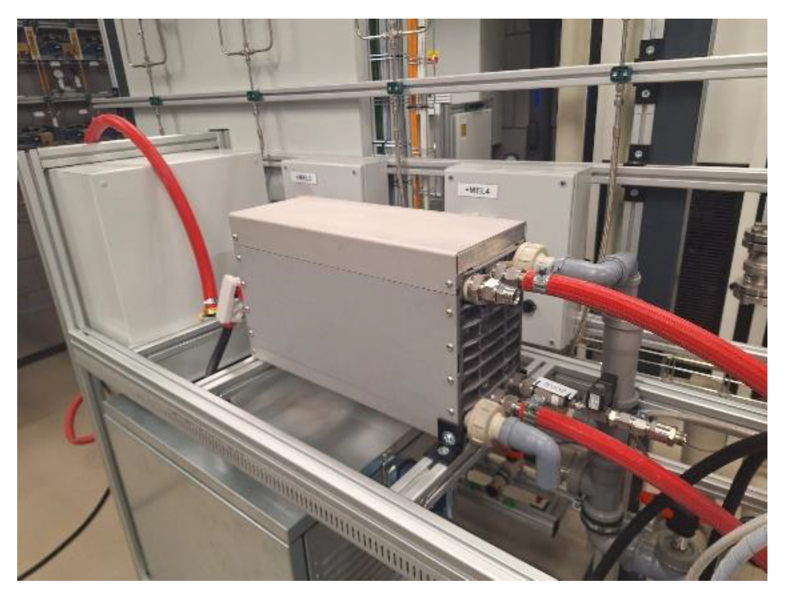
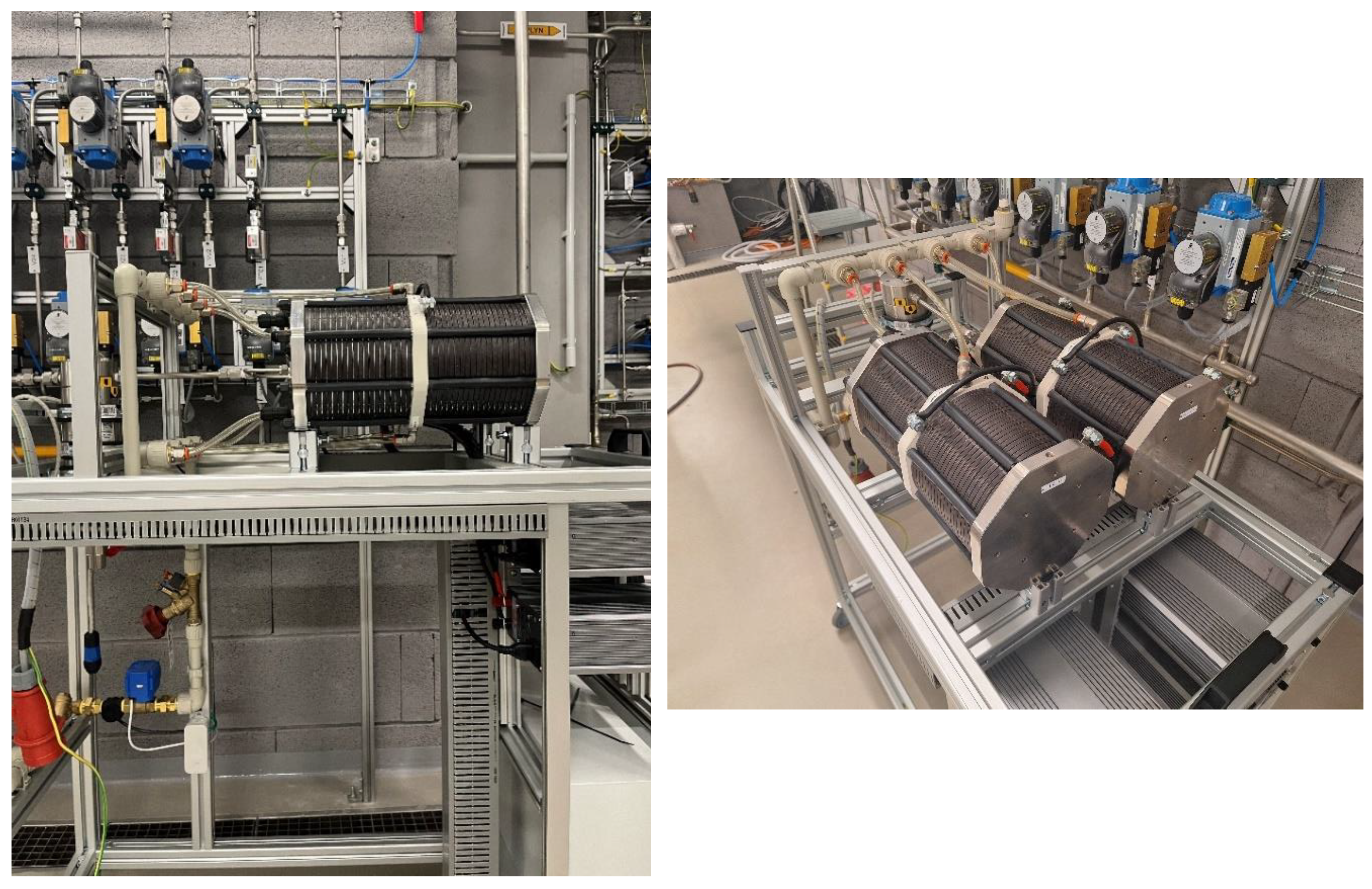
2.1.6.1. Fuel Cells
2.1.6.2. Electrolyzer
2.1.6.3. Purge Process of Fuel Cells and Electrolyzers
2.1.7. Combustion or Production of Liquid Fuel — An Alternative Process in the Gasification Facility
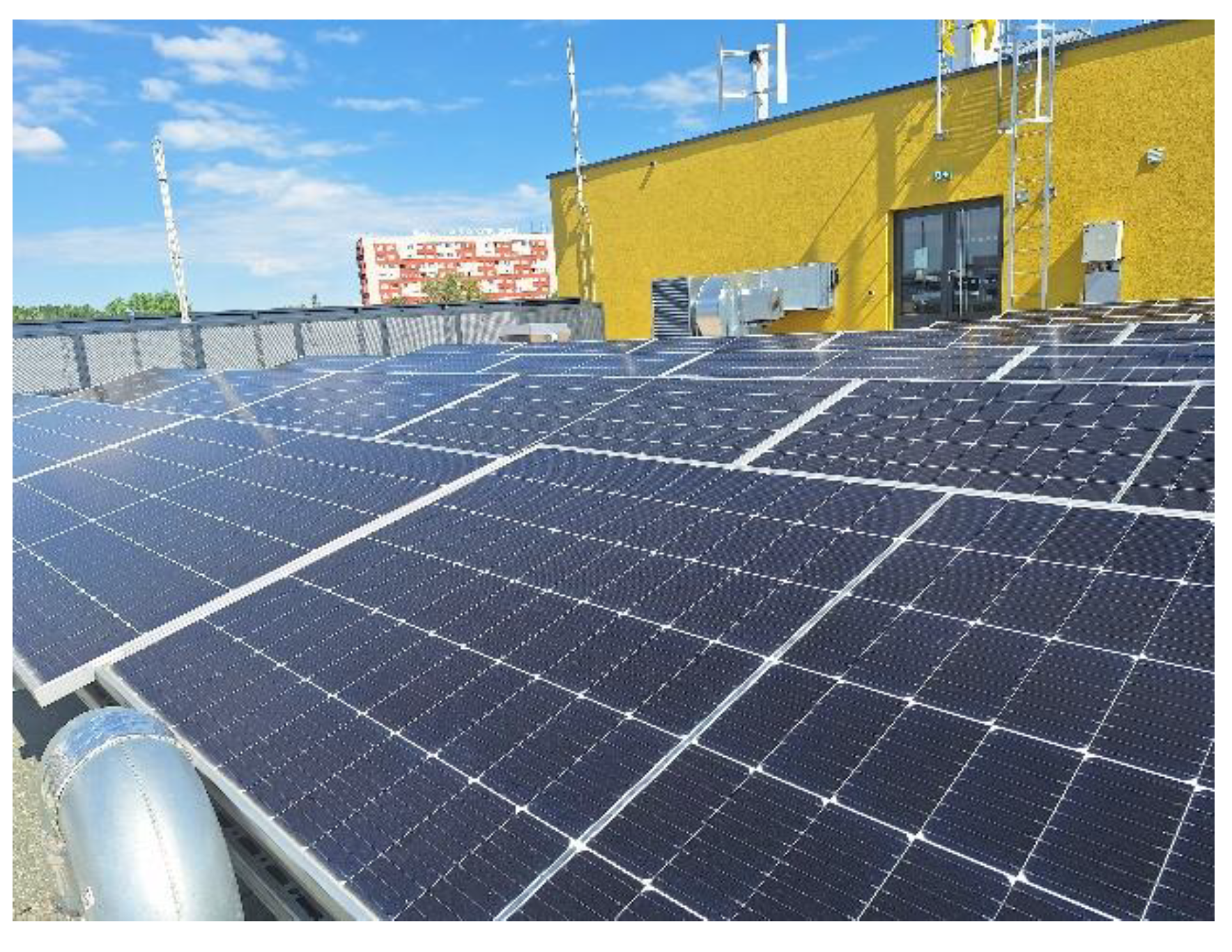
2.1.8. Photovoltaics and Wind Turbine
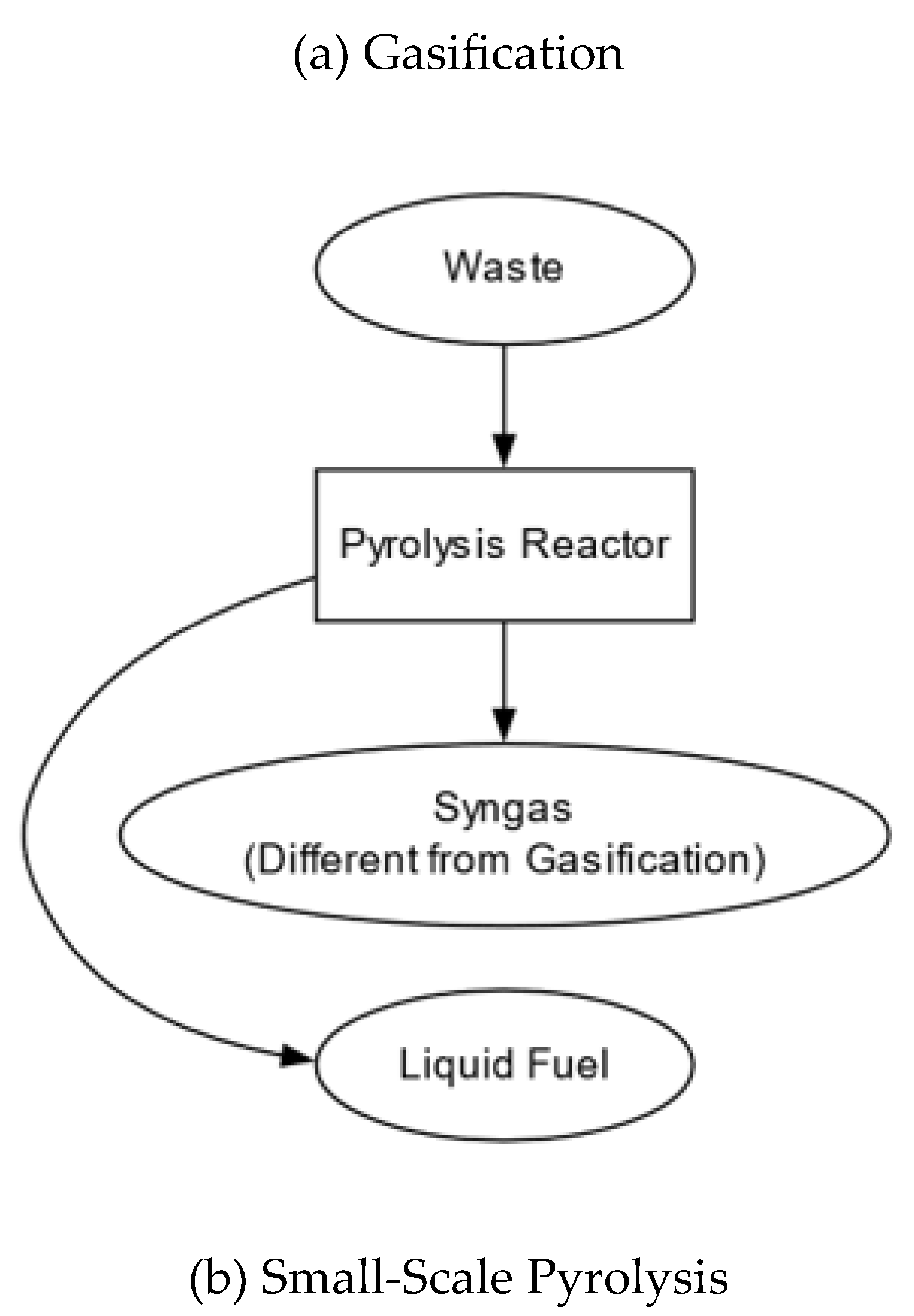
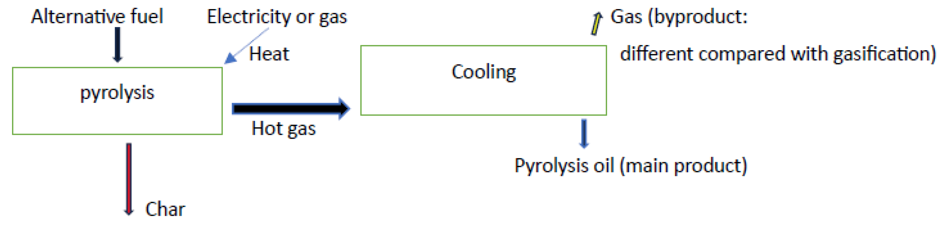
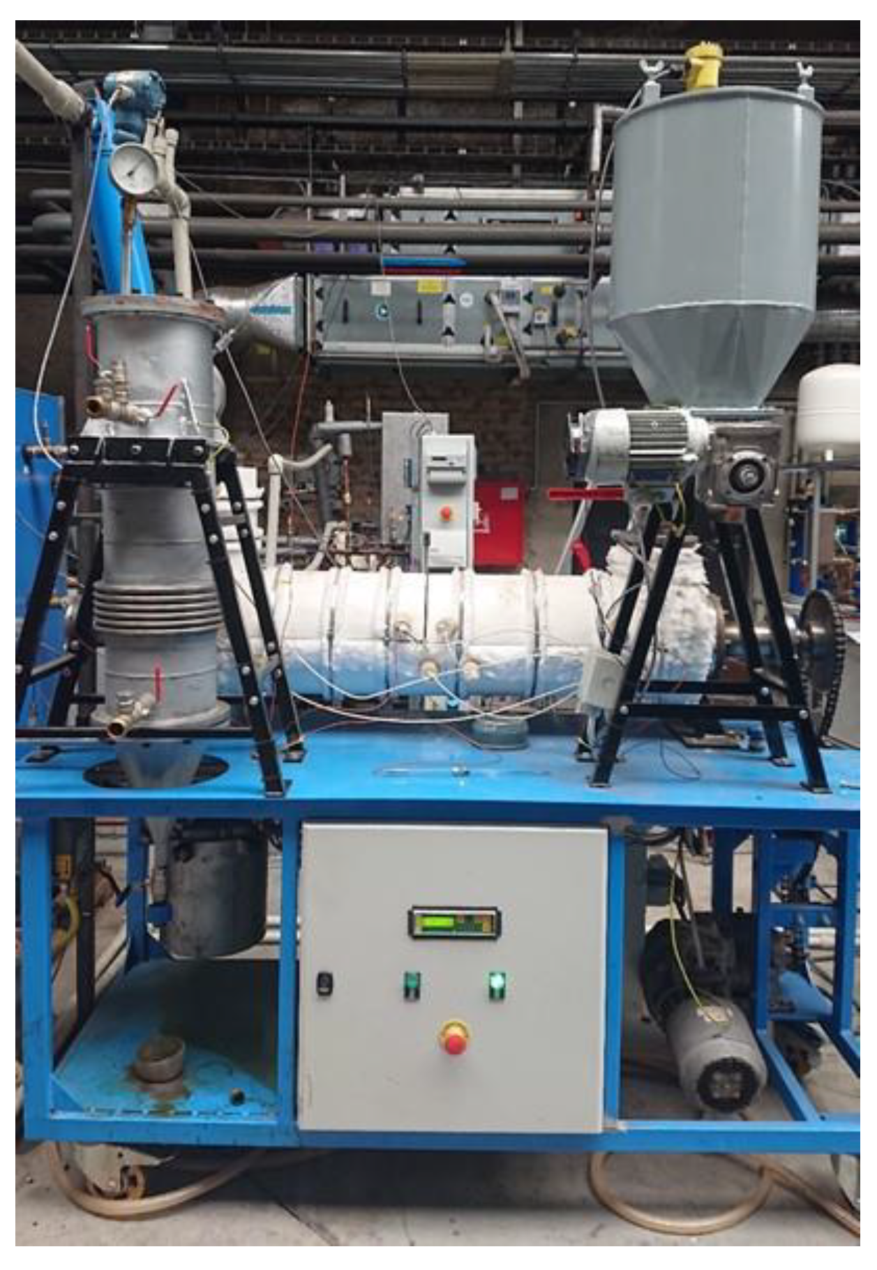
2.2. Small Pyrolysis
3. Conclusions
- Gasification: Regression methods provided interpretable and robust approximations of thermochemical processes of transforming waste to syngas, contrasting with black-box deep learning approaches. Furthermore, polynomial regression models perform better in this case compared to symbolic regression models. Optimal reactor temperature range was determined as 879–966 °C, with a peak hydrogen yield at 923 °C (H2 = 15.1%, CO2 = 11.87%, CO = 19.76%, CH4 = 2.11%, N2 = 49.3%, total 98.78%).
- Pyrolysis: the developed model identified an optimal power of 3.3 kW, converting 3 kg/h of waste input into 0.97 kg/h of liquid fuel.
- Current validation is limited by the availability of experimental datasets.
- The results are based on wood pallets typical of Central Europe; feedstock variability may affect accuracy when extending to other waste types.
- Scaling up from laboratory to industrial operation may introduce additional uncertainties related to reactor performance, energy efficiency, and emissions.
- Potential environmental and health impacts of different waste-to-energy processes require further investigation.
- The developed tools are open-source (Python, MS Excel) and accessible through web browsers, enabling interactive scenario analysis.
- The software supports community-scale applications, including industrial enterprises and municipalities, and may be integrated with renewable energy sources (PV, wind) or fuel cell systems.
- Extend datasets and validation across different waste feedstocks to improve generalizability.
- Conduct a comprehensive techno-economic analysis (similar as Rizqi [5]) to assess feasibility at different scales. Integrate cost analysis.
- Integrate environmental impact assessments (e.g., life-cycle analysis, emission control studies) into the modeling framework.
- Facilitate further transparency by releasing additional open-source data and codes.
Funding
Author Contribution Roles
Data availability
Electronic Appendices
Electronic Appendix A
Electronic Appendix B
Electronic Appendix C
Declaration of conflicting interests
Declaration of generative AI in scientific writing
Nomenclature (main text)
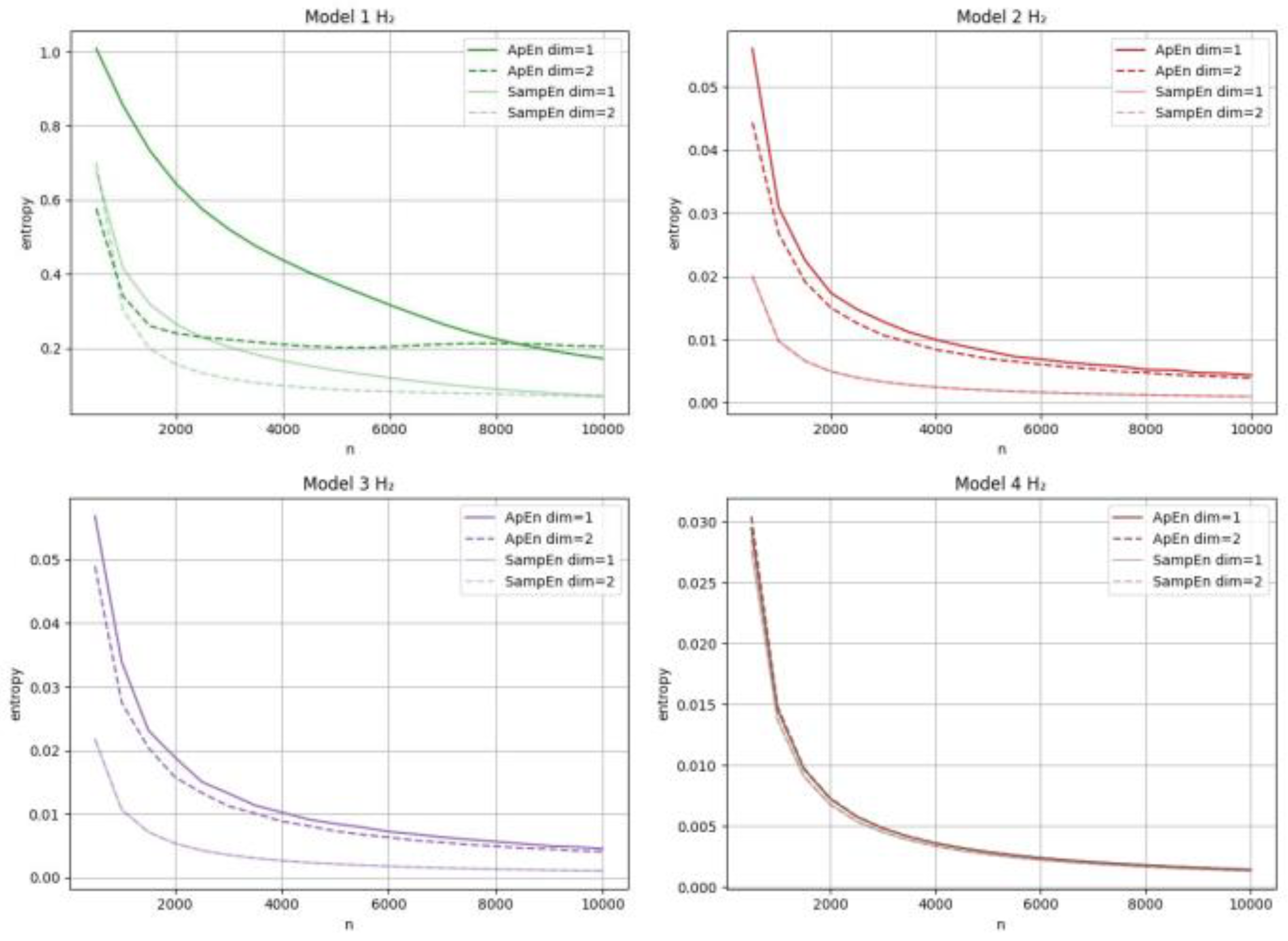
Appendix A - Evaluation of gasification models using entropy
A.1 Approximation and sample entropy
A.2 Calculation of approximate entropy
- - window length or dimension,
- - area diameter or tolerance.
A.3 Calculation of sample entropy
- is the number of pairs of vectors such that ,
- is the number of pairs of vectors such that ,
- is the Chebyshev distance.
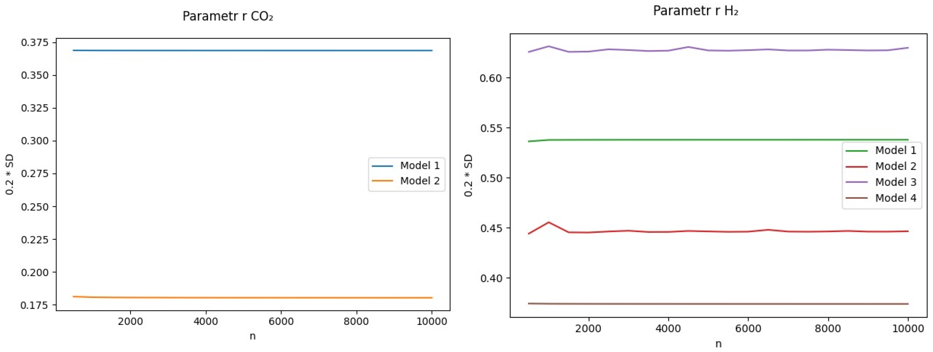
A.4 Choice of approximation and sample entropy parameters
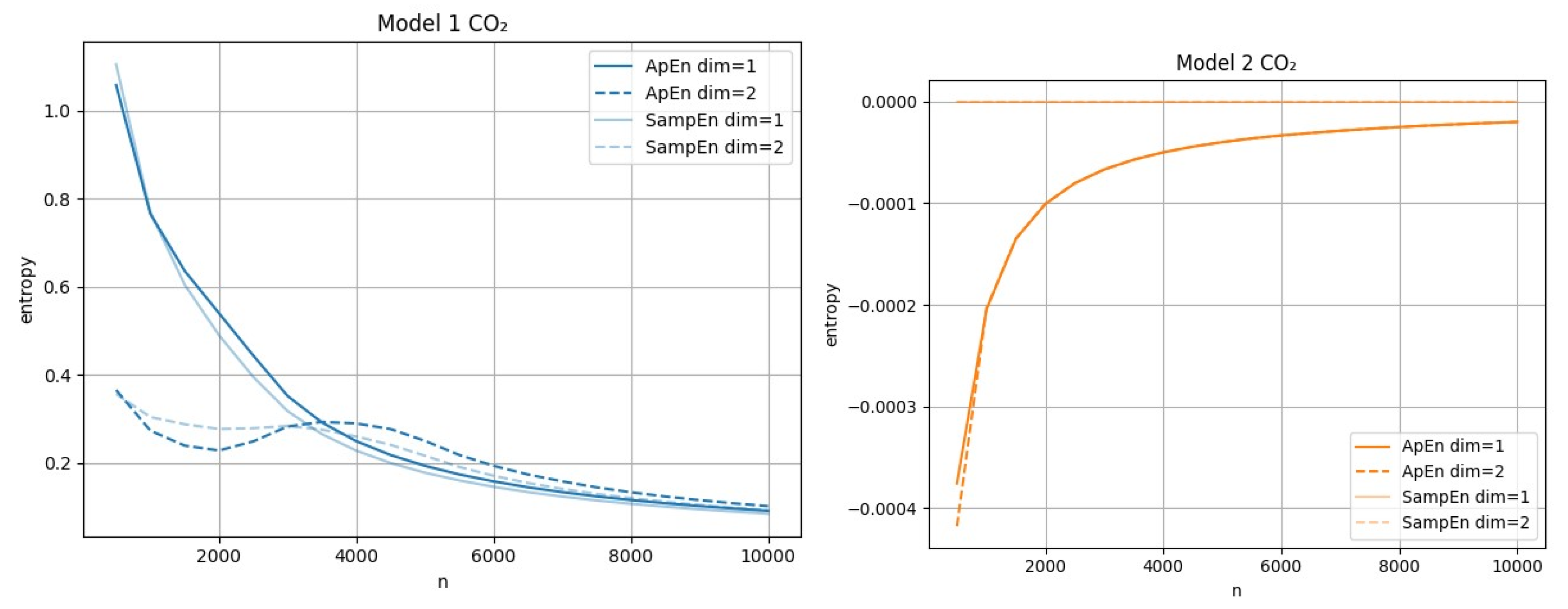
A.5 Conclusions of model evaluation using entropy
- CO2 Model 1:,
- CO2 Model 2: ,
- H2 Model 1: ,
- H2 Model 2: ,
- H2 Model 3: ,
- H2 Model 4:.

| CO2 | ApEn | SampEn |
| Model 1 | 0.10207402716557201 | 0.09283472789592226 |
| Model 2 | -1.9966127829285085e-05 | 0.0 |
| H2 | ApEn | SampEn |
| Model 1 | 0.20472909404756345 | 0.06955908463228219 |
| Model 2 | 0.003898864346688402 | 0.0009846446174318114 |
| Model 3 | 0.0040850415534996465 | 0.0010645168626448073 |
| Model 4 | 0.001447427615602681 | 0.0013493376152297486 |
Appendix B
References
- Aich, W.; Hammoodi, K.A.; Mostafa, L.; Saraswat, M.; Shawabkeh, A.; Said, L.B.; El-Shafay, A.S.; Mahdavi, A. Techno-economic and life cycle analysis of two different hydrogen production processes from excavated waste under plasma gasification. Process Saf. Environ. Prot. 2024, 184, 1158–1176. [Google Scholar] [CrossRef]
- Awodun, K.; He, Y.; Wu, C.; Soltani, S.M. Catalytic pyrolysis of bio-waste in synthesis of value-added products: A systematic review. Fuel Process. Technol. 2025, 275, 108258. [Google Scholar] [CrossRef]
- Freda, C.; Giuliano, A.; Villone, A.; Cornacchia, G.; Catizzone, E. Valorization of municipal solid waste from Marocco towards hydrogen, methanol, or electricity: An experimental and process simulation study. Fuel Process. Technol. 2025, 275, 108259. [Google Scholar] [CrossRef]
- Aziz, M.; Darmawan, A.; Juangsa, F.B. Hydrogen production from biomasses and wastes: A technological review. Int. J. Hydrog. Energy 2021, 46, 33756–33781. [Google Scholar] [CrossRef]
- Rizqi, Z.U. A simulation-based optimization approach for sustainable energy supply chain transitions. Supply Chain Anal. 2025, 27, 100150. [Google Scholar] [CrossRef]
- dos Santos, R.M.; Szklo, A.; Lucena, A.F.P.; de, M. PEV. Blue sky mining: Strategy for a feasible transition in emerging countries from natural gas to hydrogen. Int. J. Hydrog. Energy 2021, 46, 25843–25859. [Google Scholar] [CrossRef]
- Thomas, R. The development of the manufactured gas industry in Europe. Geological Society, London, Special Publications 2018, 465, 137–164. [Google Scholar] [CrossRef]
- Melaina, M.W. Market Transformation Lessons for Hydrogen from the Early History of the Manufactured Gas Industry. Chapter 5, In Hydrogen Energy and Vehicle Systems; CRC Press eBooks, 2012; pp. 150–185. [Google Scholar] [CrossRef]
- Wehrer, M.; Rennert, T.; Mansfeldt, T.; Totsche, K.U. Contaminants at former manufactured gas plants: Sources, properties, and processes. Crit. Rev. Environ. Sci. Technol. 2011, 41, 1883–1969. [Google Scholar] [CrossRef]
- Hamper, M.J. Manufactured gas history and processes. Environ. Forensics 2006, 7, 55–64. [Google Scholar] [CrossRef]
- Albertazzi, S.; Basile, F.; Brandin, J.; Einvall, J.; Hulteberg, C.; Fornasari, G.; Rosetti, V.; Sanati, M.; Trifirò, F.; Vaccari, A. The technical feasibility of biomass gasification for hydrogen production. Catal. Today 2005, 106, 297–300. [Google Scholar] [CrossRef]
- Liebs, L.H. Town gas: An overview. AGA distribution/transmission conference, Boston, Massachusetts, 1985; Available online: https://semspub.epa.gov/work/01/458914.pdf (accessed on 22 May 2024).
- Maksimov, A.L.; Ishkov, A.G.; Pimenov, A.A.; Romanov, K.V.; Mikhailov, A.M.; Koloshkin, E.A. Physico-chemical aspects and carbon footprint of hydrogen production from water and hydrocarbons. J. Min. Inst. 2024, 265, 87–94. Available online: https://pmi.spmi.ru/pmi/article/view/16363/16227 (accessed on 21 June 2024).
- Lyu, H.; He, Y.; Tang, J.; Hecker, M.; Liu, Q.; Jones, P.D.; Codling, G.; Giesy, J.P. Effect of pyrolysis temperature on potential toxicity of biochar if applied to the environment. Environ. Pollut. 2016, 218, 1–7. [Google Scholar] [CrossRef] [PubMed]
- Rutkowski, J.V.; Levin, B.C. Acrylonitrile-butadiene-styrene copolymers (ABS): Pyrolysis and combustion products and their toxicity? A review of the literature. Fire Mater. 1986, 10, 93–105. [Google Scholar] [CrossRef]
- Advances in Synthesis Gas: Methods, Technologies and Applications; Rahimpour, M.R., Makarem, M.A., Meshksar, M., Eds.; Elsevier eBooks, 2022. [Google Scholar] [CrossRef]
- Odell, W.W. Facts Relating to the Production and Substitution of Manufactured Gas for Natural Gas. Department of Commerce, Bureau of Mines. 1929. Available online: https://books.google.rs/books?id=st4RRgrGA3sC&lr&pg (accessed on 21 June 2024).
- Erdener, B.C.; Sergi, B.; Guerra, O.J.; Chueca, A.L.; Pambour, K.; Brancucci, C.; Hodge, B.M. A review of technical and regulatory limits for hydrogen blending in natural gas pipelines. Int. J. Hydrog. Energy 2023, 48, 5595–5617. [Google Scholar] [CrossRef]
- Ozturk, M.; Sorgulu, F.; Javani, N.; Dincer, I. An experimental study on the environmental impact of hydrogen and natural gas blend burning. Chemosphere 2023, 329, 138671. [Google Scholar] [CrossRef]
- Ascher, S.; Wang, X.; Watson, I.; Sloan, W.; You, S. Interpretable machine learning to model biomass and waste gasification. Bioresour. Technol. 2022, 364, 128062. [Google Scholar] [CrossRef]
- Li, J.; Li, L.; Tong, Y.W.; Wang, X. Understanding and optimizing the gasification of biomass waste with machine learning. Green Chem. Eng. 2023, 4, 123–133. [Google Scholar] [CrossRef]
- Lee, J.; Hong, S.; Cho, H.; Lyu, B.; Kim, M.; Kim, J.; Moon, I. Machine learning-based energy optimization for on-site SMR hydrogen production. Energy Convers. Manag. 2021, 244, 114438. [Google Scholar] [CrossRef]
- Chu, C.; Boré, A.; Liu, X.W.; Cui, J.C.; Wang, P.; Liu, X.; Chen, G.Y.; Liu, B.; Ma, W.C.; Lou, Z.Y.; Tao, Y. Modeling the impact of some independent parameters on the syngas characteristics during plasma gasification of municipal solid waste using artificial neural network and stepwise linear regression methods. Renew. Sustain. Energy Rev. 2022, 157, 112052. [Google Scholar] [CrossRef]
- Kaheel, S.; Ibrahim, K.A.; Fallatah, G.; Lakshminarayanan, V.; Luk, P.; Luo, Z. Advancing Hydrogen: A Closer Look at Implementation Factors, Current Status and Future Potential. Energies 2023, 16, 7975. [Google Scholar] [CrossRef]
- Hasanzadeh, R.; Mojaver, P.; Azdast, T.; Chitsaz, A.; Park, C.B. Low-emission and energetically efficient co-gasification of coal by incorporating plastic waste: A modeling study. Chemosphere 2022, 299, 134408. [Google Scholar] [CrossRef] [PubMed]
- Raj, R.; Singh, D.K.; Tirkey, J.V. Co-gasification of plastic waste blended with coal and biomass: A comprehensive review. Environ. Technol. Rev. 2023, 12, 614–642. [Google Scholar] [CrossRef]
- Smoliński, A.; Howaniec, N.; Gąsior, R.; Polański, J.; Magdziarczyk, M. Hydrogen rich gas production through co-gasification of low rank coal, flotation concentrates and municipal refuse derived fuel. Energy 2021, 235, 121348. [Google Scholar] [CrossRef]
- Zainal, B.S.; Ker, P.J.; Mohamed, H.; Ong, H.C.; Fattah, I.M.; Rahman, S.A.; Nghiem, L.D.; Mahlia, T.I. Recent advancement and assessment of green hydrogen production technologies. Renew. Sustain. Energy Rev. 2024, 189, 113941. [Google Scholar] [CrossRef]
- Oh, S.; Park, S.R.; Kang, Y.T. Optimum design of high-temperature steam generator for hydrogen production enhancement. Int. J. Energy Res. 2023, 2023, 9022385. [Google Scholar] [CrossRef]
- Chojnacki, J.; Kielar, J.; Kukiełka, L.; Najser, T.; Pachuta, A.; Berner, B.; Zdanowicz, A.; Frantík, J.; Najser, J.; Peer, V. Batch pyrolysis and co-pyrolysis of beet pulp and wheat straw. Materials 2022, 15, 1230. [Google Scholar] [CrossRef]
- Chojnacki, J.; Kielar, J.; Najser, J.; Frantík, J.; Najser, T.; Mikeska, M.; Gaze, B.; Knutel, B. Straw pyrolysis for use in electricity storage installations. Heliyon 2024, 10, e30058. [Google Scholar] [CrossRef]
- Čespiva, J.A.; Wnukowski, M.; Skřínský, J.; Perestrelo, R.; Jadlovec, M.; Výtisk, J.; Trojek, M.; Câmara, JS. Production efficiency and safety assessment of the solid waste-derived liquid hydrocarbons. Environ. Res. 2024, 244, 117915. [Google Scholar] [CrossRef]
- Vaculik, J.; Hradilek, Z.; Moldrik, P.; Minarik, D. Calculation of efficiency of hydrogen storage system at the fuel cells laboratory. In Proceedings of the 2014 15th International Scientific Conference on Electric Power Engineering (EPE); IEEE; pp. 381–384. [CrossRef]
- Najser, J.; Frantik, J. Smart Grid System Using Electricity from Photovoltaics, Renewable Sources and Alternative Fuels. In Proceedings of the ISES Solar World Congress, 2019. [Google Scholar] [CrossRef]
- Hlaba, A.; Rabiu, A.; Osibote, O.A. Thermochemical Conversion of Municipal Solid Waste—An Energy Potential and Thermal Degradation Behavior Study. Int. J. Environ. Sci. Dev. 2016, 7, 661–667. [Google Scholar] [CrossRef]
- Pacheco, N.; Ribeiro, A.; Oliveira, F.; Pereira, F.; Marques, L.; Teixeira, J.C.; Vilarinho, C.; Barbosa, F.V. Sewage sludge plasma gasification: Characterization and experimental rig design. Reactions 2024, 5, 285–304. [Google Scholar] [CrossRef]
- Kongprawes, G.; Wongsawaeng, D.; Hosemann, P.; Ngaosuwan, K.; Kiatkittipong, W.; Assabumrungrat, S. Dielectric barrier discharge plasma for catalytic-free palm oil hydrogenation using glycerol as hydrogen donor for further production of hydrogenated fatty acid methyl ester (H-FAME). J. Clean. Prod. 2023, 401, 136724. [Google Scholar] [CrossRef]
- Sarantaridis, D.; Fowowe, T.; Caruana, D.J. Electrochemistry in flames. Sci. Prog. 2010, 93, 301–317. [Google Scholar] [CrossRef] [PubMed]
- Elaissi, S.; Alsaif, N.A.M. Modeling and Performance Analysis of municipal solid waste treatment in plasma torch reactor. Symmetry 2023, 15, 692. [Google Scholar] [CrossRef]
- Leal-Quirós, E. Plasma processing of municipal solid waste. Brazilian Journal of Physics 2004, 34(4b), 1587–1593. [Google Scholar] [CrossRef]
- Dubčáková, R. Eureqa: Software review. Genet. Program. Evolvable Mach. 2010, 12, 173–178. [Google Scholar] [CrossRef]
- Brkić, D.; Praks, P.; Marek, M.; Ilić, U.; Stajić, Z. Reducing the number of input variables through symbolic regression. Electron. Res. Arch. 2025, 33, 5158–5178. [Google Scholar] [CrossRef]
- Hasanzadeh, R.; Mojaver, M.; Azdast, T.; Park, C.B. A novel systematic multi-objective optimization to achieve high-efficiency and low-emission waste polymeric foam gasification using response surface methodology and TOPSIS method. Chem. Eng. J. 2022, 430, 132958. [Google Scholar] [CrossRef]
- Čespiva, J.; Skřínský, J.; Vereš, J.; Borovec, K.; Wnukowski, M. Solid-recovered fuel to liquid conversion using fixed bed gasification technology and a Fischer–Tropsch synthesis unit – case study. Int. J. Energy Prod. Manag. 2020, 5, 212–222. [Google Scholar] [CrossRef]
- Becker, W.L.; Braun, R.J.; Penev, M.; Melaina, M. Production of Fischer–Tropsch liquid fuels from high temperature solid oxide co-electrolysis units. Energy 2012, 47, 99–115. [Google Scholar] [CrossRef]
- Zhang, K.; Harvey, A.P. CO2 decomposition to CO in the presence of up to 50% O2 using a non-thermal plasma at atmospheric temperature and pressure. Chem. Eng. J. 2021, 405, 126625. [Google Scholar] [CrossRef]
- Praks, P.; Lampart, M.; Praksová, R.; Brkić, D.; Kozubek, T.; Najser, J. Selection of appropriate symbolic regression models using statistical and dynamic system criteria: Example of waste gasification. Axioms 2022, 11, 463–463. [Google Scholar] [CrossRef]
- Chang, P.-Y.; Yang, P.-Y.; Chou, F.-I.; Chen, S.-H. Hybrid optimization algorithm for thermal displacement compensation of computer numerical control machine tool using regression analysis and fuzzy inference. Science Progress 2023, 106. [Google Scholar] [CrossRef] [PubMed]
- Udrescu, S.M.; Tegmark, M. AI Feynman: A physics-inspired method for symbolic regression. Science Advances 2020, 6. [Google Scholar] [CrossRef] [PubMed]
- Praks, P.; Brkić, D.; Najser, J.; Najser, T.; Praksová, R.; Stajić, Z. Methods of Artificial Intelligence for Simulation of Gasification of Biomass and Communal Waste. 2021 22nd International Carpathian Control Conference (ICCC), Velké Karlovice, Czech Republic, 2021. [Google Scholar] [CrossRef]
- Cranmer, M. Interpretable Machine Learning for Science with PySR and SymbolicRegression. jl 2023. [Google Scholar] [CrossRef]
- Smith, W.R.; Tahir, H.; Leal, A.M.M. Stoichiometric and non-stoichiometric methods for modeling gasification and other reaction equilibria: A review of their foundations and their interconvertibility. Renew. Sustain. Energy Rev. 2024, 189, 113935–113935. [Google Scholar] [CrossRef]
- Dell, R.M.; Moseley, P.T.; Rand, D.A.J. Chapter 8 - Hydrogen, Fuel Cells and Fuel Cell Vehicles. Towards Sustainable Road Transport 2014, 260–295. [Google Scholar] [CrossRef]
- Mekhilef, S.; Saidur, R.; Safari, A. Comparative study of different fuel cell technologies. Renew. Sustain. Energy Rev. 2012, 16, 981–989. [Google Scholar] [CrossRef]
- Wu, C.; Zhu, Q.; Dou, B.; Fu, Z.; Wang, J.; Mao, S. Thermodynamic analysis of a solid oxide electrolysis cell system in thermoneutral mode integrated with industrial waste heat for hydrogen production. Energy 2024, 301, 131678. [Google Scholar] [CrossRef]
- Martinez Lopez, V.A.; Ziar, H.; Haverkort, J.W.; Zeman, M.; Isabella, O. Dynamic operation of water electrolyzers: A review for applications in photovoltaic systems integration. Renew. Sustain. Energy Rev. 2023, 182, 113407. [Google Scholar] [CrossRef]
- Perry, R.H.; Green, D.W. Perry’s chemical engineers’ handbook, 8th ed.; McGraw-Hill: New York, 2008; ISBN 9780071422949. [Google Scholar]
- Krylova, AY. Products of the Fischer-Tropsch synthesis (A Review). Solid Fuel Chem 2014, 48, 22–35. [Google Scholar] [CrossRef]
- Konstandopoulos, A.G.; Syrigou, M.; Pagkoura, C.; Sakellariou, K.; Lorentzou, S.; et al. Solar fuels and industrial solar chemistry. In Concentrating Solar Power Technology; Elsevier, 2021; pp. 677–724. [Google Scholar] [CrossRef]
- Chakraborty, J.P.; Singh, S.; a Maity, S.K. Advances in the conversion of methanol to gasoline. In Hydrocarbon Biorefinery; Elsevier, 2022; pp. 177–200. [Google Scholar] [CrossRef]
- Kalkreuth, W.; Ruaro Peralba, M.; Barrionuevo, S.; Hinrichs, R.; Silva, T.; Maman Anzolin, H.; Osório, E.; Pohlmann, J.; De Caumia, B.; Pakdel, H.; Roy, C. Vacuum Pyrolysis of Brazilian coal, peat and biomass–Results on characterization of feedstock, solid residues, pyrolysis liquids and conversion rates. Energy Explor. Exploit. 2024, 42, 817–836. [Google Scholar] [CrossRef]
- Du, Y.; Ju, T.; Meng, Y.; Han, S.; Jiang, J. Pyrolysis characteristics of excavated waste and generation mechanism of gas products. J. Clean. Prod. 2022, 370, 133489–133489. [Google Scholar] [CrossRef]
- Çelik, A.; Othman, I.B.; Müller, H.; Lott, P.; Deutschmann, O. Pyrolysis of biogas for carbon capture and carbon dioxide-free production of hydrogen. React. Chem. Eng. 2024, 9, 108–118. [Google Scholar] [CrossRef]
- Aldeia, G.S.I.; de França, F.O. Interpretability in symbolic regression: A benchmark of explanatory methods using the Feynman data set. Genet. Program. Evolvable Mach. 2022, 23, 309–349. [Google Scholar] [CrossRef]
- Praks, P.; Rasmussen, A.; Lye, K.O.; Martinovič, J.; Praksová, R.; Watson, F.; Brkić, D. Sensitivity analysis of parameters for carbon sequestration: Symbolic regression models based on open porous media reservoir simulators predictions. Heliyon 2024, 10, e40044. [Google Scholar] [CrossRef]
- Staš, M.; Auersvald, M.; Kejla, L.; Vrtiška, D.; Kroufek, J.; Kubička, D. Quantitative analysis of pyrolysis bio-oils: A review. TrAC Trends Anal. Chem. 2020, 126, 115857. [Google Scholar] [CrossRef]
- Xin, Q.; Farooqi, H.; Lang, J.; Al-Haj, B.; Saborimanesh, N. Behavioral and toxicological impacts of bio-derived oils in aqueous spills. J. Environ. Chem. Eng. 2024, 12, 114353. [Google Scholar] [CrossRef]
- Chatterjee, N.; Eom, H.J.; Jung, S.H.; Kim, J.S.; Choi, J. Toxic potentiality of bio-oils, from biomass pyrolysis, in cultured cells and Caenorhabditis elegans. Environ. Toxicol. 2014, 29, 1409–1419. [Google Scholar] [CrossRef]
- Chai, C.H.; Chan, C.Y.; Heng, J.Z.; Tang, K.Y.; Loh, X.J.; Li, Z.; Ye, E. Converting plastic waste to fuel and fine chemicals. In InCircularity of Plastics; Elsevier, 1 Jan 2023; pp. 71–100. [Google Scholar] [CrossRef]
- Flood, MW. EntropyHub. Available online: https://www.entropyhub.xyz/.
- Buchlovská Nagyová, J.; Jansík, B.; Lampart, M. Detection of embedded dynamics in the Györgyi-Field model. Sci. Rep. 2020, 10(21031), s41598–s020.77874–77876. [Google Scholar] [CrossRef]
- Lampart, M.; Vantuch, T.; Zelinka, I.; Mišák, S. Dynamical properties of partial-discharge patterns. International Journal of Parallel, Emergent and Distributed Systems 2018, 33, 474–489. [Google Scholar] [CrossRef]
- Lampart, M.; Zapoměl, J. Motion of an unbalanced impact body colliding with a moving belt. Mathematics 2021, 9, 1071. [Google Scholar] [CrossRef]
| 1 | Extended analysis is given in Appendix A. |
| 2 | |
| 3 | Electrolyzer modeling for green hydrogen: https://www.gridcog.com/blog/electrolyser-modelling-for-green-hydrogen (accessed on June 28, 2024). |
| 4 | These scripts are given in Appendix B. |
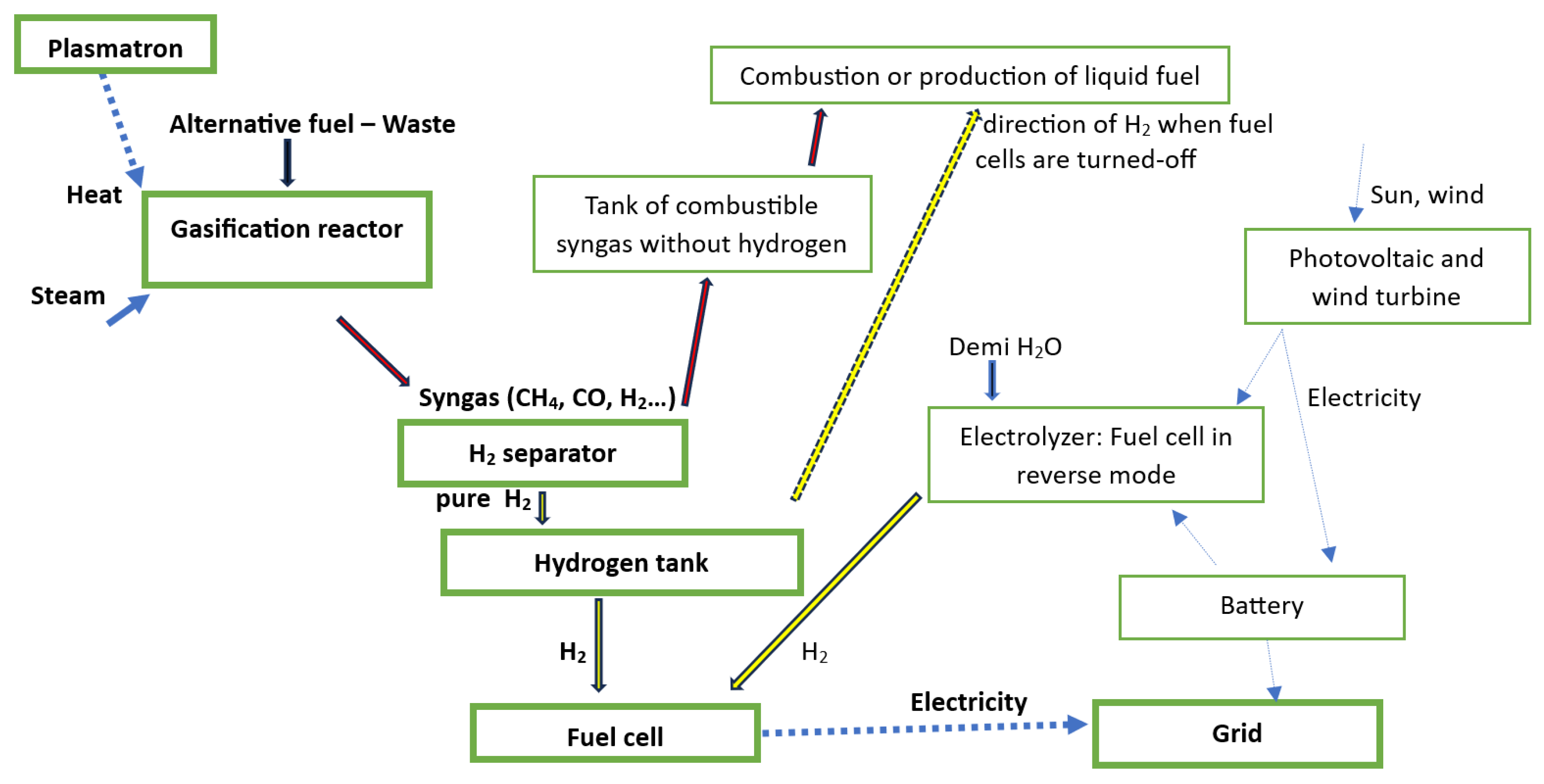
| aMain process | Input | Output |
| Plasmatron | Nozzle base constant k [dimensionless] | Middle plasma torch temperature T [K] |
| Plasma torch power P [kW] | ||
| Filling pressure of air fp [bar] | ||
| Gasification reactor | Alternative fuel – Waste | Syngas |
| Heat c (Middle plasma temperature T [K] transformed to temperature in the gasification reactor t [°C]) | Waste residual | |
| Steam, i.e., water | ||
| Hydrogen separator | Syngas | Pure hydrogen |
| Syngas without hydrogen | ||
| Hydrogen tank | Hydrogen from Hydrogen separator | Hydrogen |
| Fuel cells | Hydrogen from Gasification | d Electricity |
| Hydrogen from Electrolyzer | ||
| Auxiliary process | Input | Output |
| Electrolyzer | Electricity (from Battery or Photovoltaics/Wind turbine) | Hydrogen |
| Water (Demi water) | ||
| b Alternative process | Input | Output |
| Tank of combustible syngas without hydrogen | Syngas without hydrogen | Combustible syngas without hydrogen |
| Non-combustible compounds of syngas | ||
| Combustion | Combustible syngas without hydrogen | Heat |
| Hydrogen | ||
| Production of liquid fuel | Combustible syngas without hydrogen | Liquid fuel |
| Non-combustible components of syngas | ||
| Hydrogen |
| Gas compound | normal m3 | Number of mol | Mass of gas [kg] | Mass % | Composition Vol. % |
| H2 | ≈ 3.5 | 154.5 | ≈ 0.3 | ≈ 1.5 | 19.7 |
| CO2 | ≈ 2 | 88.9 | ≈ 3.9 | ≈ 19.5 | 11.3 |
| CO | ≈ 3.7 | 163.4 | ≈ 4.6 | ≈ 22.8 | 20.8 |
| CH4 | ≈ 0.4 | 17.5 | ≈ 0.3 | ≈ 1.4 | 2.2 |
| N2 | ≈ 8.8 | 393.4 | ≈ 11 | ≈ 54.8 | 50.1 |
| Σ | ≈ 18.3 | 818.0 | ≈ 20 | 100 | 104.1 |
| Gas compound | Number of mol n | nR [m3·Pa/K] | known T [K] | Known V [m3] | p [bar] |
| H2 | 154.5 | 1284.9 | 50 | 5 | ≈ 0.13 |
| CO2 | 88.9 | 739.8 | 50 | 5 | ≈ 0.07 |
| CO | 163.4 | 1359.3 | 50 | 5 | ≈ 0.14 |
| CH4 | 17.5 | 145.7 | 50 | 5 | ≈ 0.01 |
| N2 | 393.4 | 3271.3 | 50 | 5 | ≈ 0.33 |
| Σ | 818.0 | 6801.2 | 50 | 5 | ≈ 0.68 |
| a Gas compound | Number of mol | nR [m3·Pa/K] | known p [bar] | Known V [m3] | T [K] |
| H2 | 154.5 | 1284.9 | 41.5 | 5 | 16176.8 |
| CO2 | 88.9 | 739.8 | 37.3 | 5 | 25244.7 |
| CO | 163.4 | 1359.3 | 138.1 | 5 | 50801.3 |
| CH4 | 17.5 | 145.7 | 19.6 | 5 | 67237.1 |
| N2 | 393.4 | 3271.3 | 202.7 | 5 | 30985.7 |
| Σ | 818.0 | 6801.2 | 439.3 | 5 | 32301.0 |
| a Gas compound | Number of mol | nR [m3·Pa/K] | known p [bar] | known T [K] | V [m3] |
| H2 | 154.5 | 1284.9 | 41.5 | 50 | ≈ 0.015 |
| CO2 | 88.9 | 739.8 | 37.3 | 50 | ≈ 0.010 |
| CO | 163.4 | 1359.3 | 138.1 | 50 | ≈ 0.005 |
| CH4 | 17.5 | 145.7 | 19.6 | 50 | ≈ 0.004 |
| N2 | 393.4 | 3271.3 | 202.7 | 50 | ≈ 0.008 |
| Σ | 818.0 | 6801.2 | 439.3 | 50 | ≈ 0.008 |
| Gas compound in vol. % | |||||
| Temperature t [°C] in gasification reactor | CO2 | H2 | CO | CH4 | N2 |
| 750 | 8.1 | 9.7 | 29.4 | 4.4 | 45.2 |
| 800 | 9.8 | 10.9 | 26.0 | 4.0 | 46.2 |
| 900 | 11.9 | 16.0 | 20.1 | 2.2 | 48.4 |
| 1000 | 11.3 | 12.8 | 19.9 | 1.7 | 52.8 |
| 1050 | 11.5 | 12.3 | 18.8 | 1.2 | 55.0 |
| 1100 | 12.3 | 11.8 | 12.4 | 1.0 | 56.3 |
| Gas compound in % vol. | Model - Formula where t [°C] is the middle temperature in the gasification reactor |
| Polynomial regression 5 degree – Used in the final version of the developed waste-to-energy software | |
| H2 | |
| CO2 | |
| CO | |
| CH4 | |
| N2 | |
| Symbolic regression: Models obtained in PySR – Used in the final version of the developed waste-to-energy software | |
| H2 | =LN(ABS(0.000677729241918855×t^2×ABS(LN(ABS(0.0010822109×t)+0.00000001))^(-2.6401255))+0.00000001) |
| CO2 | =LN(ABS(-0.060511474×t^2+44.81684×t)+0.00000001)+2.0503674 |
| CO | =0.7548879×t/(0.07978012×t-40.459797) |
| CH4 | =ABS(3.6089828-3679.8438/(t-300.00784)) |
| N2 | =ABS(0.000001013×t-0.0017925174)^(-0.5535527) |
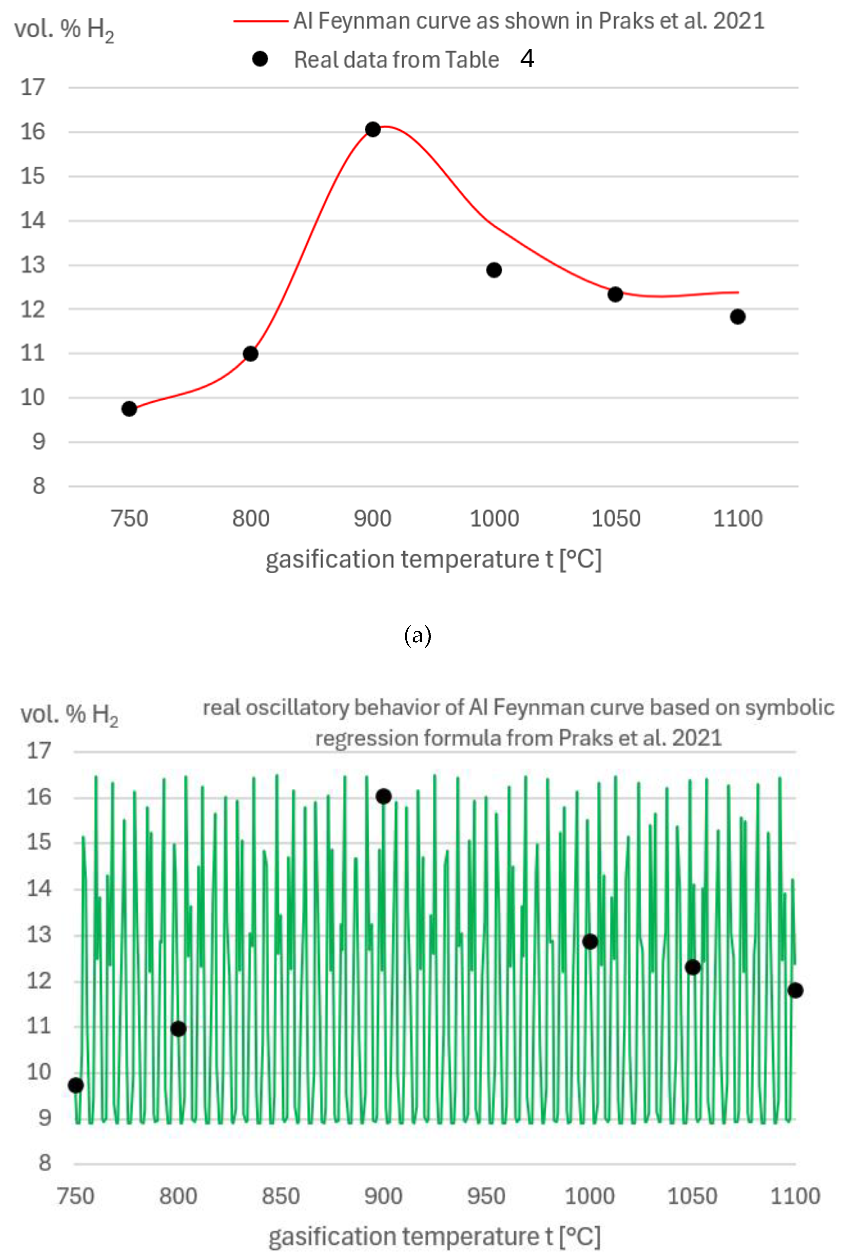
| Symbolic regression: AI Feynman with oscillatory tendencies [50] – Rejected for use after reanalysis | |
| H2 | 1/(0.112277210469×COS(COS(((EXP(SIN((t+1)))-1)-1)))) |
| CO2 | Model 1: 0.003263060755×(t×LN((SQRT(t)+SIN(LN(t))))) Model 2: TAN(-29.286471691464+SQRT(((t×EXP(COS((LN(t)+1))))-1))) |
| CO | 6.719797422959×EXP(EXP(SIN((((COS(t)-1))^(-1)+1)))) |
| CH4 | (0.946772291789×(EXP(COS((EXP(SIN((t+t)))+1)))+1))^2 |
| N2 | SQRT(-664.727896959755×((((COS(EXP(COS(t)))-1)-1)-1)-1)) |
| Used in the evaluation in Appendix A of this article | |
| Model 1 CO2 | , |
| Model 2 CO2 | , |
| Model 1 H2 | |
| Model 2 H2 |
, |
| Model 3 H2 |
, |
| Model 4 H2 | Repeated model for H2 from above in this Table from polynomial regression 5 degree |
| Polynomial degree | Hydrogen H2 |
| 2 | -1.369-4 t2+0.258 t-106,612 |
| 3 | 4.358-7 t3-0.001 t2+1.372 t-444.415 |
| 4 | 7.734-9 t4-2.828-5 t3+0.038 t2-22.876t+5070.377 |
| 5 | 6.251-12 t5-2.139-8 t4+2.573-5 t3-0.011t2-2.718-5 t+890.767 |
| 6 | 5.077-15 t6-1.661-11 t5+1.865-8 t4-7.344-6 t3-2.149-8 t2+4.614-11 t+246.526 |
| Polynomial degree | Carbon dioxide CO2 |
| 2 | -4.6710-5 t2+0.096t-37.252 |
| 3 | 4.21510-7 t3-0.001t2+1.173t-363.929 |
| 4 | 1.82410-9 t4-6.3510-6 t3+0.008t2-4.545t+936.676 |
| 5 | 1.23710-12 t5-3.94510-9 t4+4.35910-6 t3-0.002t2-4.13610-6 t+105.442 |
| 6 | 7.53410-16 t6-2.17710-12 t5+2.07110-9 t4-6.42210-7 t3-1.8810-9 t2+4.03410-12 t+6.226 |
| Polynomial degree | Carbon monoxide CO |
| 2 | 1.01710-4t2-0.219t+136.345 |
| 3 | -5.87310-7 t3+0.002t2-1.721t+591.542 |
| 4 | -3.80710-9 t4+1.35510-5 t3-0.018t2+10.215t-2123.132 |
| 5 | -2.74210-12 t5+9.02410-9 t4-1.03610-5 t3+0.004t2+1.02910-5 t-248.532 |
| 6 | -1.8510-15 t6+5.67210-12 t5-5.8510-9 t4+2.04810-6 t3+5.99510-9 t2-1.28710-11 t-0.241 |
| Polynomial degree | Methane CH4 |
| 2 | 1.88510-5 t2-0.045t+27.658 |
| 3 | 2.83810-8 t3-6.01210-5 t2+0.028t+5.659 |
| 4 | -1.28610-9 t4+4.80310-6 t3-0.007t2+4.06t-911.393 |
| 5 | -1.08110-12 t5+3.78310-9 t4-4.65910-6 t3+0.002t2+5.03210-6 t-164.977 |
| 6 | -9.13510-16 t6+3.06210-12 t5-3.52510-9 t4+1.42110-6 t3+4.1610-9 t2-8.92810-12 t-44.059 |
| Polynomial degree | Nitrogen N2 |
| 2 | 3.80110-5t2-0.037t+51.345 |
| 3 | -2.67910-7 t3+0.001t2-0.722t+258.964 |
| 4 | -2.41210-9 t4+8.68710-6 t3-0.012t2+6.841t-1461.047 |
| 5 | -1.94110-12 t5+6.54510-9 t4-7.7710-6 t3+0.003t2+8.15510-6 t-222.896 |
| 6 | -1.59710-15 t6+5.16710-12 t5-5.75510-9 t4+2.27110-6 t3+6.64710-9 t2-1.42710-11 t-34.106 |
| Polynomial | degree 2 | degree 3 | a degree 4 | degree 5 | degree 6 |
| Max. absolute error | |||||
| CO2 | 1.05 | 0.69 | 0.48 | 0.49 | 0.51 |
| H2 | 1.9 | 2.09 | 1.07 | 1.13 | 1.18 |
| CO | 1.48 | 1.43 | 0.87 | 0.91 | 0.96 |
| CH4 | 0.57 | 0.54 | 0.54 | 0.55 | 0.56 |
| N2 | 1.51 | 1.42 | 1.53 | 1.52 | 1.51 |
| Max. relative (percentage) error | |||||
| CO2 | 13.0 | 9.0 | 6.0 | 6.0 | 6.0 |
| H2 | 20.0 | 22.0 | 11.0 | 12.0 | 12.0 |
| CO | 9.0 | 8.0 | 5.0 | 5.0 | 6.0 |
| CH4 | 62.0 | 57.9 | 59.0 | 60.0 | 61.0 |
| N2 | 3.0 | 3.0 | 3.0 | 3.0 | 3.0 |
| Mean squared error | |||||
| CO2 | 0.27 | 0.07 | 0.04 | 0.04 | 0.04 |
| H2 | 1.09 | 0.87 | 0.3 | 0.35 | 0.39 |
| CO | 0.75 | 0.35 | 0.21 | 0.22 | 0.23 |
| CH4 | 0.06 | 0.06 | 0.04 | 0.04 | 0.05 |
| N2 | 0.63 | 0.54 | 0.49 | 0.49 | 0.49 |
| Inputsa | Outputs b | |||||||
| Combination | k [[-] | P [kW] | fp [bar] | T [K] | t [°C] | c Syngas produced [m³/h] | vol. H2 % | |
| 1. | 9.6 | 15 | 3 | 10621.9 | 925 | 17.6 | 15.9 | |
| 2 | 5 | 9.9 | 3.8 | 10621.9 | 925 | 17.6 | 15.9 | |
| 3 | 8.9 | 15 | 3.3 | 10429.3 | 921.3 | 17.6 | 15.9 | |
| 4 | 5 | 7.5 | 3 | 10225.0 | 917.4 | 17.6 | 15.9 | |
| ⁞ | ⁞ | ⁞ | ⁞ | ⁞ | ⁞ | ⁞ | ⁞ | |
| a the base constant of nozzle k [no units] from 5 to 20, required power of plasma torch P [kW] from 5 to 15, and filling pressure [bar] from 3 to 8 Used unrealistic peak in symbolic regression is 22.5 % vol. of hydrogen; b T [K] is the middle temperature of the plasma torch, while t [°C] is the temperature in the gasification reactor; c for waste input 20 kg/h (e.g., waste input 5 kg/h gives 4.4 m3/h of syngas) | ||||||||
| k [[-] | P [kW] | fp [bar] | Waste input [kg/h] | Syngas produced [m³/h] | vol. H2 % | H2 produced [m³/h] | Tank | ||
| Pressure [bar] | Temperature [K] | Filling time [h] | |||||||
| 9.6 | 15 | 3 | 20 | 17.6 | 15.9 | 2.79 | 100 | 200 | 107 |
| 5 | 9.9 | 3.8 | 5 | 4.4 | 15.9 | 0.70 | 160 | 220 | 623 |
| 8.9 | 15 | 3.3 | 10 | 8.8 | 15.9 | 1.40 | 200 | 250 | 343 |
| 8.9 | 15 | 3.3 | 17 | 15.0 | 15.9 | 2.38 | 200 | 298 | 169 |
| 13.4 | 9.4 | 6.4 | 16 | 14.1 | 10.5 | 1.48 | 200 | 298 | 276 |
| 9.7 | 11.3 | 4.9 | 20 | 17.6 | 12.8 | 2.25 | 200 | 298 | 182 |
| ⁞ | ⁞ | ⁞ | ⁞ | ⁞ | ⁞ | ⁞ | ⁞ | ⁞ | ⁞ |
| k [[-] | P [kW] | fp [bar] | Waste input [kg/h] | Mass of H2 [kg/h] | a Power of fuel cells [kW] | Efficiency [%] | Output — Obtained electrical energy [kWh] | |
| b LHV=33kWh/kg | c HHV=39.38kWh/kg | |||||||
| 9.6 | 15 | 3 | 20 | 0.39 | 40 | 50 | 6.4 | 7.6 |
| 5 | 9.9 | 3.8 | 5 | 0.10 | 40 | 40 | 1.3 | 1.5 |
| 8.9 | 15 | 3.3 | 10 | 0.17 | 40 | 36 | 2.0 | 2.4 |
| 8.9 | 15 | 3.3 | 17 | 0.29 | 40 | 36 | 3.4 | 4.1 |
| 13.4 | 9.4 | 6.4 | 16 | 0.13 | 40 | 60 | 2.6 | 3.1 |
| 9.7 | 11.3 | 4.9 | 20 | 0.19 | 32 | 60 | 3.7 | 4.4 |
| ⁞ | ⁞ | ⁞ | ⁞ | ⁞ | ⁞ | ⁞ | ⁞ | ⁞ |
| a Electricity input [kWh] | Hydrogen produced [kg] | |||
| Photovoltaics and wind | Grid | From photovoltaics and wind | From grid | |
| 14 | 54 | 0.27 | 1.04 | |
| 20 | 20 | 0.38 | 0.38 | |
| 17 | 7 | 0.33 | 0.13 | |
| ⁞ | ⁞ | ⁞ | ⁞ | |
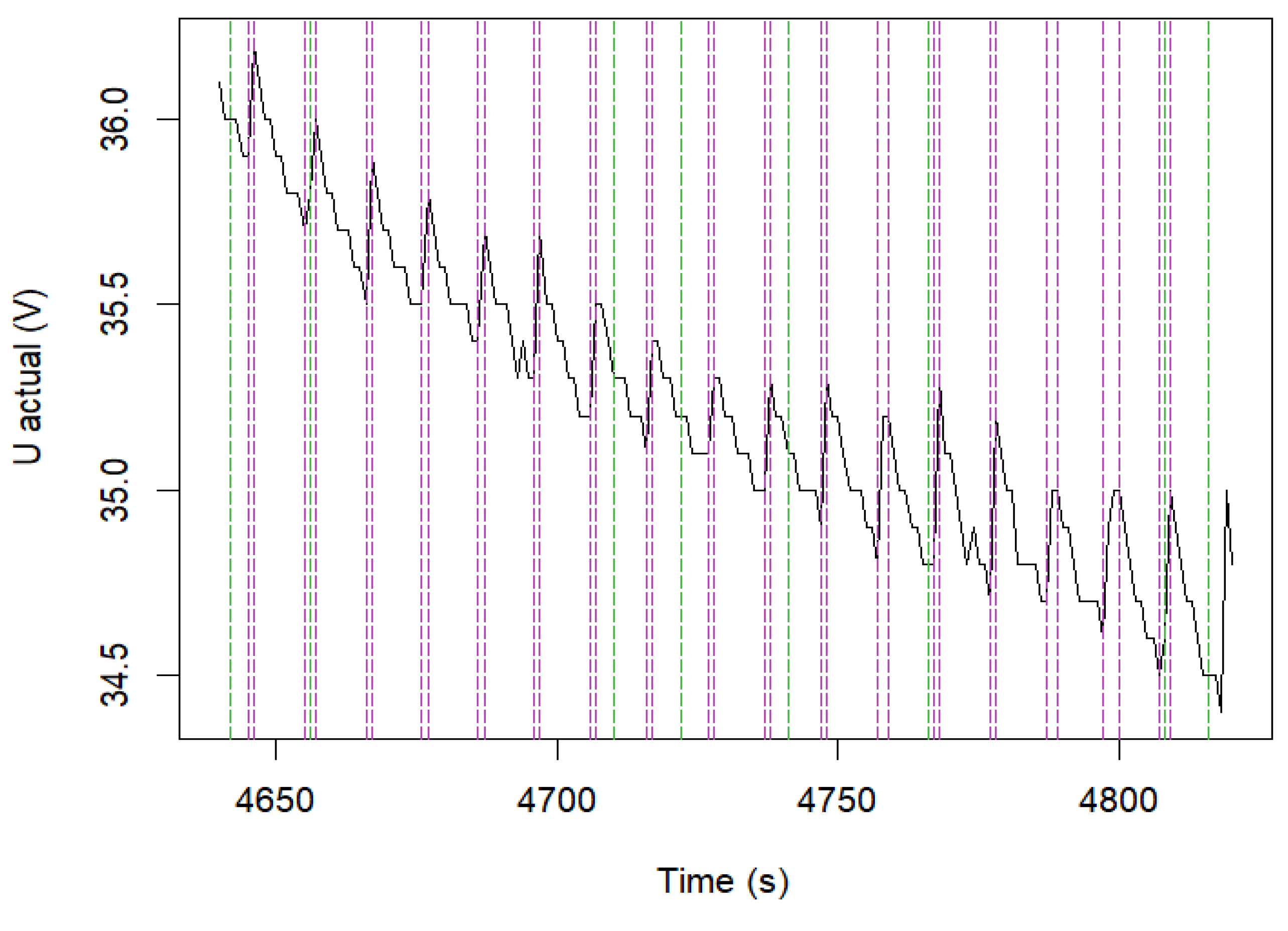
| aAmount of hydrogen produced | |||
| Interval | Actual (dm3/min) | Prediction (dm3/min) | Absolute error (dm3/min) |
| 1 | 40.73 | 40.73 | 0 |
| 2 | 20.69 | 20.63 | 0.06 |
| 3 | 19.75 | 19.83 | 0.08 |
| 4 | 29.84 | 29.84 | 0 |
| 5 | 28.02 | 28.01 | 0.01 |
| 6 | 28.78 | 28.56 | 0.22 |
| 7 | 28.40 | 28.68 | 0.28 |
| 8 | 30.39 | 32.92 | 2.53 |
| 9 | 2.62 | 0.09 | 2.53 |
| 10 | 26.28 | 28.53 | 2.25 |
| 11 | 36.70 | 34.06 | 2.64 |
| 12 | 29.69 | 30.23 | 0.54 |
| 13 | 31.39 | 31.18 | 0.21 |
| 14 | 30.75 | 31.08 | 0.33 |
| 15 | 34.79 | 34.79 | 0 |
| 16 | 30.23 | 30.23 | 0 |
| a Component of syngas | Produced kg/hours | Ideal theoretical 100% efficiency | 35% efficiency | |||
| kWh – HHV | kWh – LHV | kWh – HHV | kWh – LHV | |||
| H2 | 0.53 | 21.05 | 17.79 | 7.37 | 6.23 | |
| CO | 16.88 | 47.63 | 47.63 | 16.67 | 16.67 | |
| CH4 | 1.39 | 21.34 | 19.21 | 7.47 | 6.72 | |
| Electricity from | Battery capacity [kWh] | а Consumed by | ||||
| Photovoltaics [kW] | Wind turbine [kW] | Battery [kWh] | Time to fill up the battery [hours] | |||
| 120 | 5 | 500 | 108 | 4.6 | ||
| 60 | 7 | 500 | 50 | 10 | ||
| 60 | 7 | 600 | 50 | 12 | ||
| 120 | 3 | 700 | 106 | 6.6 | ||
| ⁞ | ⁞ | ⁞ | ⁞ | ⁞ | ||
| Input | Output | |
| Pyrolysis reactor | Alternative fuel – Waste | Hot gas |
| Heat (through electricity or gas) | Char | |
| Cooling | Hot gas | Pyrolysis oil (liquid fuel) — Main product |
| Syngas (different than syngas from gasification) — Byproduct |
| Gas compound | mass. % |
| CO2 | 76.631-0.0309×t-0.000070876×t2 |
| CO | 71.64571-0.18489×t+0.00018×t2 |
| CH4 | -35.957+0.1855×t-0.00014×t2 |
| H2 | -10.5349+0.0235×t+0.0000336×t2 |
| Input | Output | |||||||
| Electricity [kWh] | Waste [kg/h] | Pyrolysis temperature t [°C] | Pyrolysis oil (Liquid fuel) L [kg] | Char [kg] | Gas G [kg] | |||
| 5.4 | 3 | 494.1 | 0.85 | 1.16 | 0.99 | Example 1 | ||
| 3.3 | 5 | 316.2 | 1.61 | 1.50 | 1.89 | Example 2 | ||
| ⁞ | ⁞ | ⁞ | ⁞ | ⁞ | ⁞ | ⁞ | ||
| Example 1 | Composition Vol. % | Volume [m3] | Mol | Mass [%] | Mass [kg] |
| CO2 | 44.5 | 0.3 | 14.6 | 65.1 | 0.64 |
| CO | 24.5 | 0.2 | 8.0 | 22.8 | 0.23 |
| CH4 | 21.7 | 0.2 | 7.1 | 11.6 | 0.11 |
| H2 | 9.4 | 0.1 | 3.0 | 0.6 | 0.01 |
| Σ | 100 | 0.7 | 32.9 | 100 | 0.99 |
| Example 2 | Composition Vol. % | Volume [m3] | Mol | Mass [%] | Mass [kg] |
| CO2 | 59.8 | 0.5 | 24.5 | 72.2 | 1.08 |
| CO | 31.2 | 0.3 | 12.7 | 24.0 | 0.36 |
| CH4 | 8.7 | 0.1 | 3.5 | 3.8 | 0.06 |
| H2 | 0.3 | 0.0 | 0.1 | 0.0 | 0.00 |
| Σ | 100 | 0.9 | 41.0 | 100 | 1.5 |
Disclaimer/Publisher’s Note: The statements, opinions and data contained in all publications are solely those of the individual author(s) and contributor(s) and not of MDPI and/or the editor(s). MDPI and/or the editor(s) disclaim responsibility for any injury to people or property resulting from any ideas, methods, instructions or products referred to in the content. |
© 2025 by the authors. Licensee MDPI, Basel, Switzerland. This article is an open access article distributed under the terms and conditions of the Creative Commons Attribution (CC BY) license (http://creativecommons.org/licenses/by/4.0/).


